6. Frequency-Domain Analysis of Discrete-

Time Signals and Systems

6.1. Properties of Sequence exp(jn) (1.3.3)

6.2. Definition of Discrete-Time Fourier Series (3.6)

6.3. Properties of Discrete-Time Fourier Series (3.7)

6.4. Definition of Discrete-Time Fourier Transform (5.0-5.2)

6.5. Properties of Discrete-Time Fourier Transform (5.3-5.7)

6.6. Frequency Response (3.2, 3.8, 5.4)

6.7. Linear Constant-Coefficient Difference Equations (5.8)

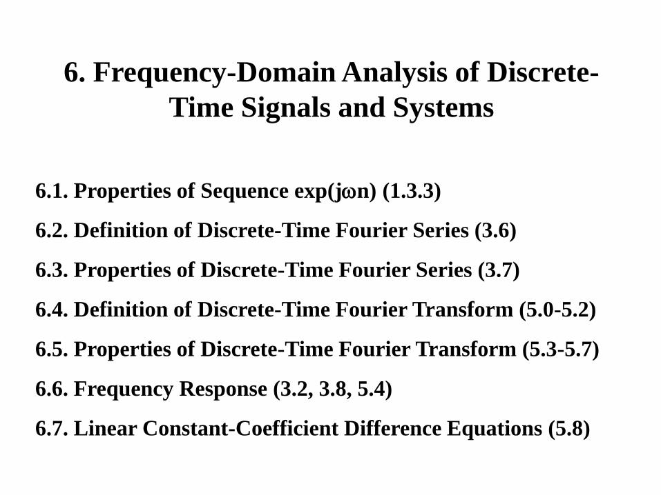
6.1. Properties of Sequence exp(jn)

6.1.1. Periodicity of Sequence exp(jn)

The sequence exp(jn) is periodic if and only if can be written

as

,N

k2 (6.1)

where k and N are integers. It can be shown that N is a period of the

sequence. If N>0, and k and N have no factors in common, N will be

the fundamental period of the sequence. Note that exp(jt) is always

periodic.

Example. Determine the periodicity of the following signals:

(1) x(t)=cos(t).

(2) x(t)=exp(jt).

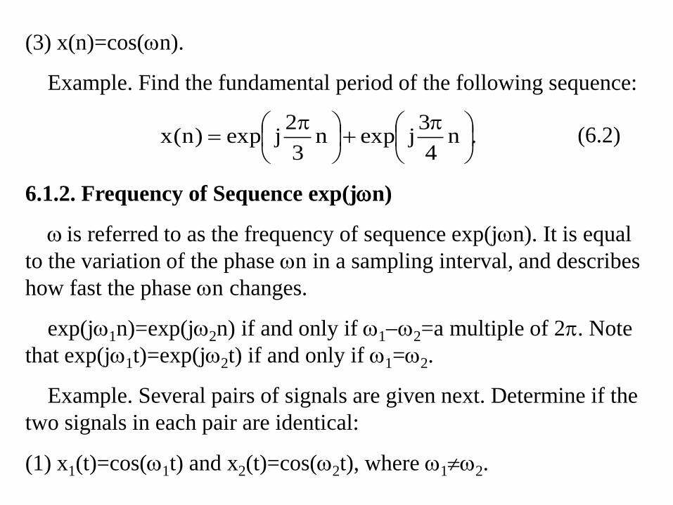
(3) x(n)=cos(n).

Example. Find the fundamental period of the following sequence:

6.1.2. Frequency of Sequence exp(jn)

is referred to as the frequency of sequence exp(jn). It is equal

to the variation of the phase n in a sampling interval, and describes

how fast the phase n changes.

exp(j1n)=exp(j2n) if and only if 12=a multiple of 2. Note

that exp(j1t)=exp(j2t) if and only if 1=2.

Example. Several pairs of signals are given next. Determine if the

two signals in each pair are identical:

(1) x1(t)=cos(1t) and x2(t)=cos(2t), where 12.

.n4

3jexpn

3

2jexp)n(x

(6.2)

(2) x1(t)=exp(j1t) and x2(t)=exp(j2t), where 12.

(3) x1(n)=cos(1n) and x2(n)=cos(2n), where 12.

Two concepts need to be clarified: (1) n is the normalized time. If t

and T are the physical time and the sampling interval, respectively,

then

n=t/T. (6.3)

(2) is actually the normalized frequency. Assume that and T are

the physical frequency and the sampling interval, respectively. Then,

=T. (6.4)

6.2. Definition of Discrete-Time Fourier Series

6.2.1. Definition

Any sequence x(n) with period N can be represented by a discrete-

time Fourier series, i.e.,

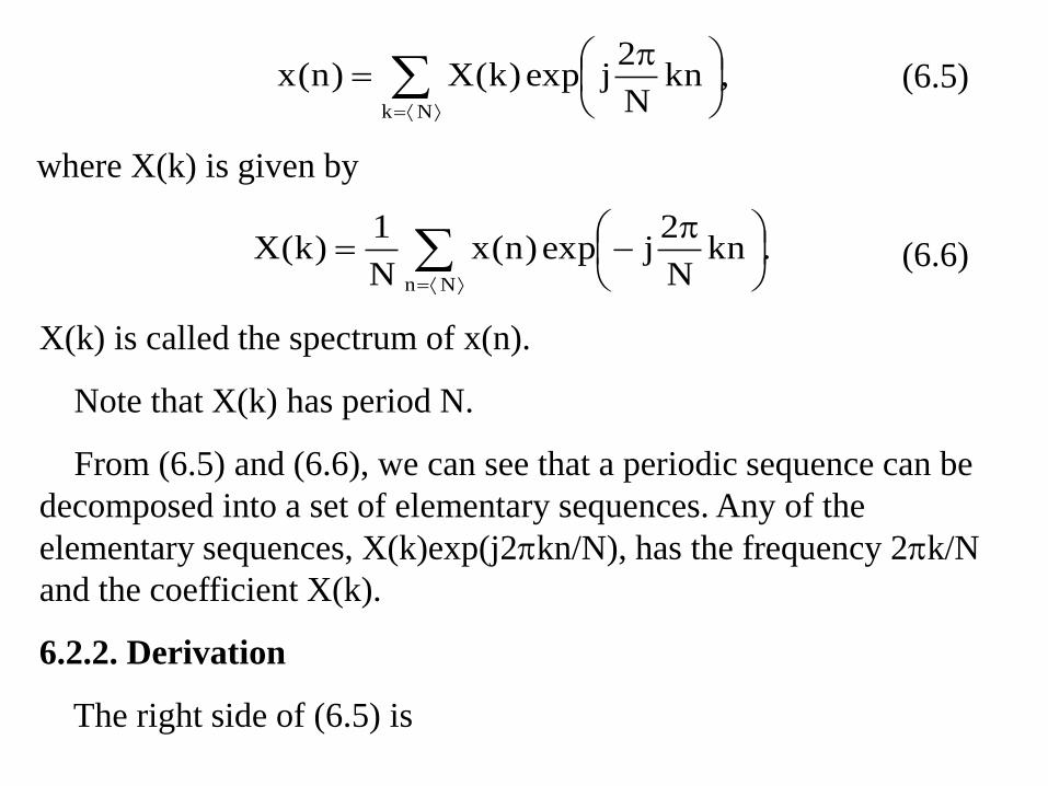
,knN

2jexp)k(X)n(x

Nk

(6.5)

where X(k) is given by

X(k) is called the spectrum of x(n).

Note that X(k) has period N.

From (6.5) and (6.6), we can see that a periodic sequence can be

decomposed into a set of elementary sequences. Any of the

elementary sequences, X(k)exp(j2kn/N), has the frequency 2k/N

and the coefficient X(k).

6.2.2. Derivation

The right side of (6.5) is

.knN

2jexp)n(x

N

1)k(X

Nn

(6.6)

.)nn(kN

2jexp

N

1)n(x

)nn(kN

2jexp

N

1)n(x

knN

2jexpnk

N

2jexp)n(x

N

1

knN

2jexp)k(X

1Nn

nn

1N

0k

Nn Nk

Nk Nn

Nk

(6.7)

Since

,1Nnnn ,0

nn ,1)nn(k

N

2jexp

N

1 1N

0k

(6.8)

(6.7) is equal to x(n).

Example. Determine the Fourier series coefficients for each of the

following signals:

(1) x(n)=sin(2Mn/N), where M and N have no common factors and

M<N.

(2) x(n)=1+sin(2n/N)+3cos(2n/N)+cos(4n/N+/2), where N5.

(3) x(n) is shown in figure 6.1.

0

Figure 6.1. A Periodic Sequence.

n

1

6.3. Properties of Discrete-Time Fourier Series

6.3.1. Linearity

Let’s assume that x1(n) and x2(n) have the same period, and a1 and

a2 are two arbitrary constants. If x1(n)X1(k) and x2(n)X2(k), then

M M NN

……

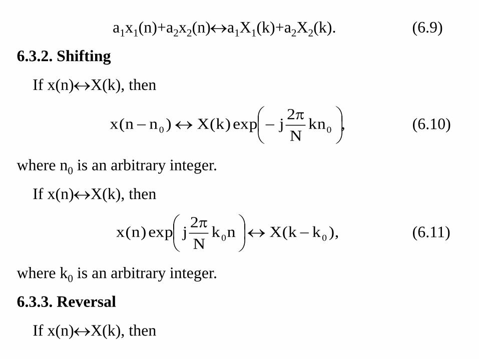
a1x1(n)+a2x2(n)a1X1(k)+a2X2(k). (6.9)

6.3.2. Shifting

If x(n)X(k), then

,knN

2jexp)k(X)nn(x 00

(6.10)

where n0 is an arbitrary integer.

If x(n)X(k), then

),kk(XnkN

2jexp)n(x 00

(6.11)

where k0 is an arbitrary integer.

6.3.3. Reversal

If x(n)X(k), then

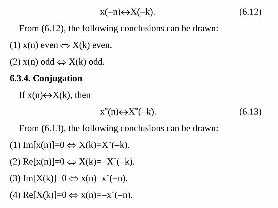
x(n)X(k). (6.12)

From (6.12), the following conclusions can be drawn:

(1) x(n) even X(k) even.

(2) x(n) odd X(k) odd.

6.3.4. Conjugation

If x(n)X(k), then

x*(n)X*(k). (6.13)

From (6.13), the following conclusions can be drawn:

(1) Im[x(n)]=0 X(k)=X*(k).

(2) Re[x(n)]=0 X(k)=X*(k).

(3) Im[X(k)]=0 x(n)=x*(n).

(4) Re[X(k)]=0 x(n)=x*(n).

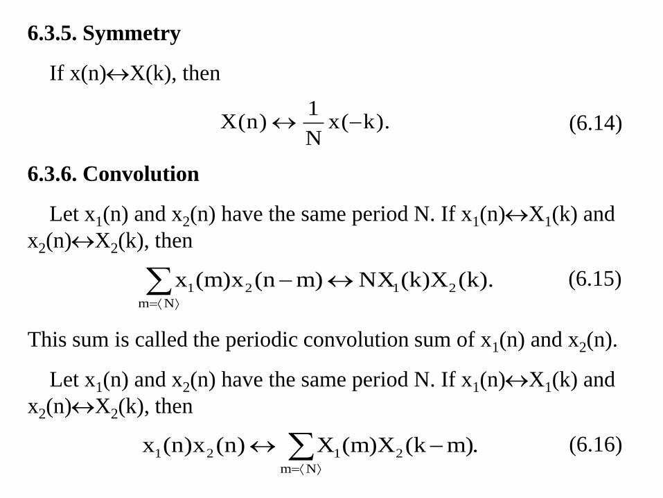
6.3.5. Symmetry

If x(n)X(k), then

).k(xN

1)n(X (6.14)

6.3.6. Convolution

Let x1(n) and x2(n) have the same period N. If x1(n)X1(k) and

x2(n)X2(k), then

).k(X)k(NX)mn(x)m(x 21

Nm

21

(6.15)

This sum is called the periodic convolution sum of x1(n) and x2(n).

Let x1(n) and x2(n) have the same period N. If x1(n)X1(k) and

x2(n)X2(k), then

.)mk(X)m(X)n(x)n(xNm

2121

(6.16)

This sum is the periodic convolution sum of X1(k) and X2(k).

6.3.7. Parseval’s Equation

If x(n)X(k), then

.)k(X)n(xN

1

Nk

2

Nn

2

(6.17)

6.4. Definition of Discrete-Time Fourier Transform

A sequence x(n) can be represented by a discrete-time Fourier

integral, i.e.,

,dnjexp)(X2

1)n(x

2

(6.18)

where X() is given by

(6.19) .njexp)n(x)(Xn

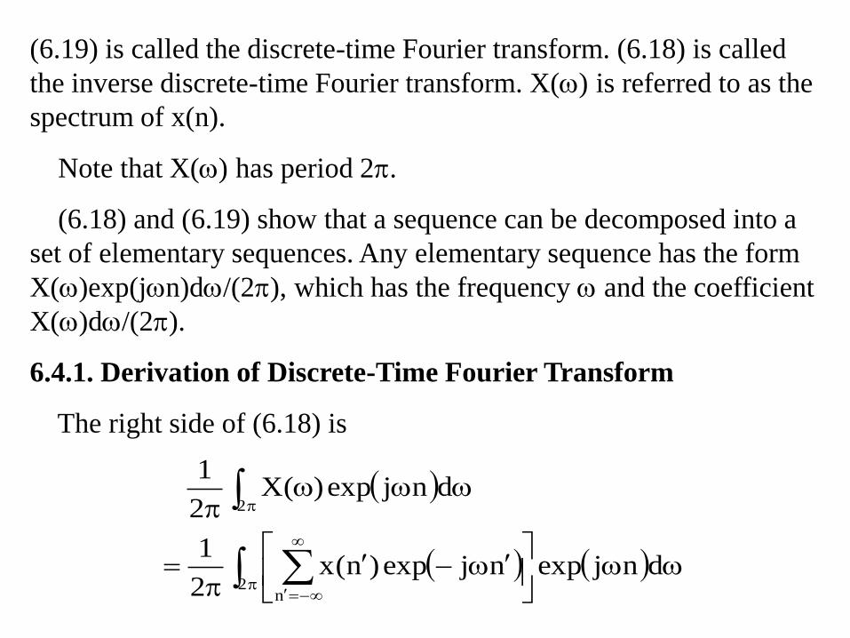
(6.19) is called the discrete-time Fourier transform. (6.18) is called

the inverse discrete-time Fourier transform. X() is referred to as the

spectrum of x(n).

Note that X() has period 2.

(6.18) and (6.19) show that a sequence can be decomposed into a

set of elementary sequences. Any elementary sequence has the form

X()exp(jn)d/(2), which has the frequency and the coefficient

X()d/(2).

6.4.1. Derivation of Discrete-Time Fourier Transform

The right side of (6.18) is

2n

2

dnjexpnjexp)n(x2

1

dnjexp)(X2

1

.d)nn(jexp2

1)n(x

n2

),nn(d)nn(jexp2

1

2

(6.21)

(6.20) becomes

).n(x)nn()n(xn

(6.22)

6.4.2. Convergence of Discrete-Time Fourier Transform

The series in (6.19) converges when x(n) is absolutely summable.

That is, there exists a finite constant B such that

Since

(6.20)

(6.23).B|)n(x|n

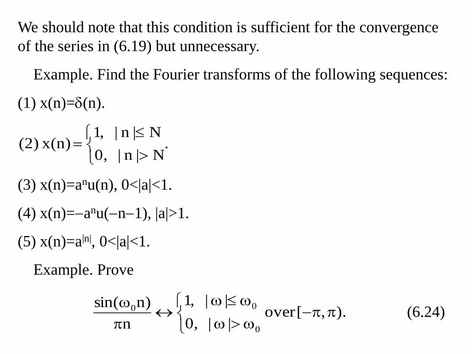
We should note that this condition is sufficient for the convergence

of the series in (6.19) but unnecessary.

Example. Find the Fourier transforms of the following sequences:

(1) x(n)=(n).

.N|n| 0,

N|n| ,1 x(n)(2)

(3) x(n)=anu(n), 0<|a|<1.

(4) x(n)=anu(n1), |a|>1.

(5) x(n)=a|n|, 0<|a|<1.

Example. Prove

(6.24)).,[ over || 0,

|| ,1

n

n)sin(

0

00

Example. Find the Fourier transform of x(n)=cos(0n).

Example. Assume that x(n) has period N and X(k) is the Fourier

series coefficient of x(n). Show that the Fourier transform of x(n) is

.kN

22)k(X)(X

k

(6.26)

6.5. Properties of Discrete-Time Fourier Transform

6.5.1. Linearity

If x1(n)X1() and x2(n)X2(), then

a1x1(n)+a2x2(n)a1X1()+a2X2(), (6.27)

where a1 and a2 are two arbitrary constants.

.m22)njexp(m

00

(6.25)

Example. Prove

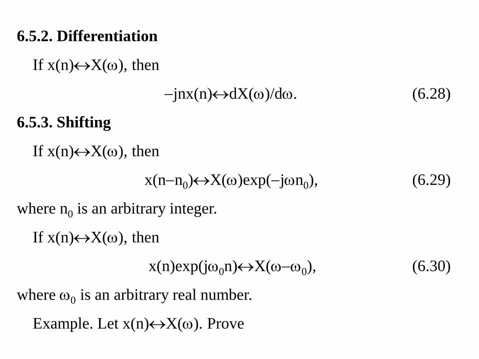
6.5.2. Differentiation

If x(n)X(), then

jnx(n)dX()/d. (6.28)

6.5.3. Shifting

If x(n)X(), then

x(nn0)X()exp(jn0), (6.29)

where n0 is an arbitrary integer.

If x(n)X(), then

x(n)exp(j0n)X(0), (6.30)

where 0 is an arbitrary real number.

Example. Let x(n)X(). Prove

6.5.4. Scaling

If x(n)X(), then

),m(X)(Ym of multiple an ,0

m of multiple an ),m/n(x)n(y

(6.32)

where m is a nonzero integer.

Letting m=1 in (6.32), we can obtain the reversal property of the

discrete-time Fourier transform, i.e.,

x(n)X(). (6.33)

From (6.33), the following conclusions can be drawn:

.

2 of multiple a ),0()0(X

2 of multiple a ,e1

)(X

)(Y)m(x)n(y jn

m

(6.31)

(1) x(n) even X() even.

(2) x(n) odd X() odd.

6.5.5. Conjugation

If x(n)X(), then

x*(n)X*(). (6.34)

From (6.34), the following conclusions can be drawn:

(1) Im[x(n)]=0 X()=X*().

(2) Re[x(n)]=0 X()=X*().

(3) Im[X()]=0 x(n)=x*(n).

(4) Re[X()]=0 x(n)=x*(n).

6.5.6. Convolution

If x1(n)X1() and x2(n)X2(), then

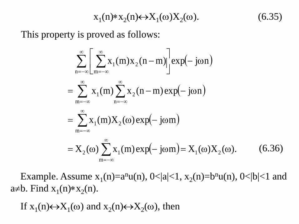
x1(n)x2(n)X1()X2(). (6.35)

This property is proved as follows:

).(X)(Xmjexp)m(x)(X

mjexp)(X)m(x

njexp)mn(x)m(x

njexp)mn(x)m(x

21

m

12

m

21

m n

21

n m

21

(6.36)

Example. Assume x1(n)=anu(n), 0<|a|<1, x2(n)=bnu(n), 0<|b|<1 and

ab. Find x1(n)x2(n).

If x1(n)X1() and x2(n)X2(), then

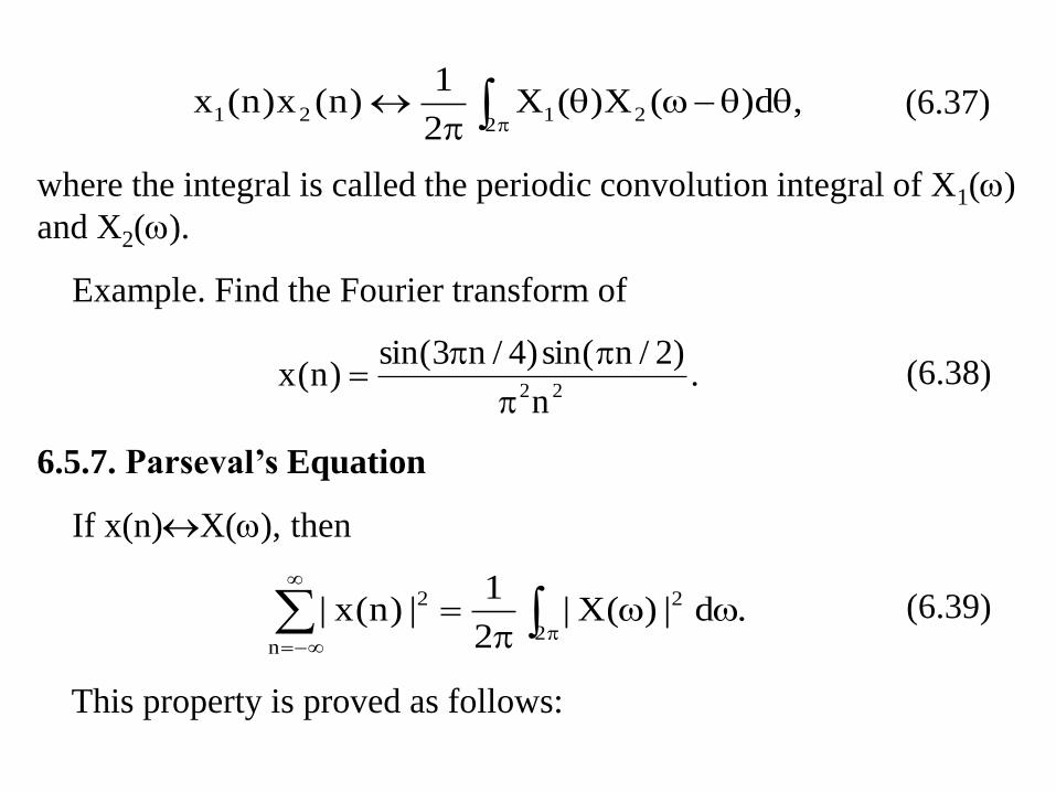
,d)(X)(X2

1)n(x)n(x

22121

(6.37)

where the integral is called the periodic convolution integral of X1()

and X2().

Example. Find the Fourier transform of

.d|)(X|2

1|)n(x|

2

2

n

2

(6.39)

This property is proved as follows:

.n

)2/nsin()4/n3sin()n(x

22

6.5.7. Parseval’s Equation

If x(n)X(), then

(6.38)

.d|)(X|2

1d)(X)(X

2

1

dnjexp)n(x)(X2

1

dnjexp)(X2

1)n(x

)n(x)n(x|)n(x|

2

2

2

*

2n

*

n

*

2

n

*

n

2

(6.40)

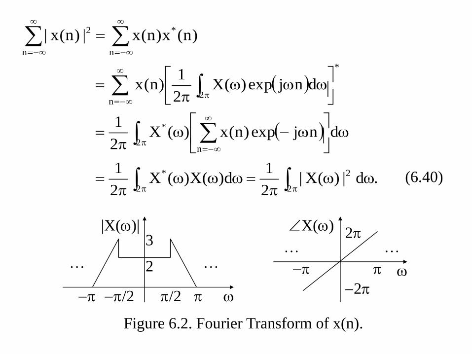
Figure 6.2. Fourier Transform of x(n).

2

3

/2 /2

|X()|

X()2

2

…… …

…

Example. Let the Fourier transform of x(n) be given in figure 6.2.

Determine whether x(n) is periodic, real, even and of finite energy.

6.6. Frequency Response

A linear time-invariant discrete-time system can be characterized

by the frequency response, which is defined as the Fourier transform

of the impulse response.

Note that the frequency response has period 2.

6.6.1. Response to exp(j0n)

Let x(n)=exp(j0n) be the input of a linear time-invariant discrete-

time system. Then, the output of the system is

y(n)=exp(j0n)H(0), (6.41)

where H() is the frequency response of the system.

Proof. Let h(n) be the impulse response of the system. Then,

).(H)njexp()mjexp()m(h)njexp(

)mn(jexp)m(h)n(y

00

m

00

m

0

(6.42)

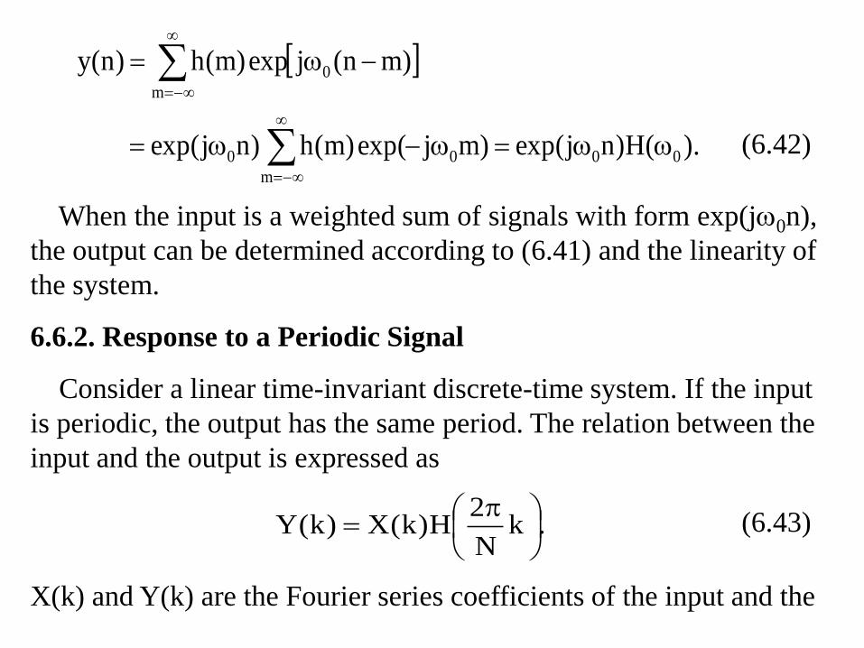
When the input is a weighted sum of signals with form exp(j0n),

the output can be determined according to (6.41) and the linearity of

the system.

6.6.2. Response to a Periodic Signal

Consider a linear time-invariant discrete-time system. If the input

is periodic, the output has the same period. The relation between the

input and the output is expressed as

.kN

2H)k(X)k(Y

(6.43)

X(k) and Y(k) are the Fourier series coefficients of the input and the

output, respectively. H() is the frequency response of the system. N

is the period.

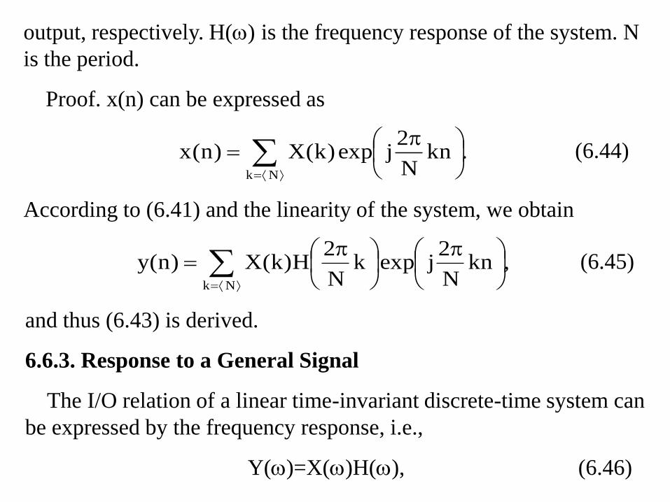
Proof. x(n) can be expressed as

.knN

2jexp)k(X)n(x

Nk

(6.44)

According to (6.41) and the linearity of the system, we obtain

and thus (6.43) is derived.

6.6.3. Response to a General Signal

The I/O relation of a linear time-invariant discrete-time system can

be expressed by the frequency response, i.e.,

Y()=X()H(), (6.46)

,knN

2jexpk

N

2H)k(X)n(y

Nk

(6.45)

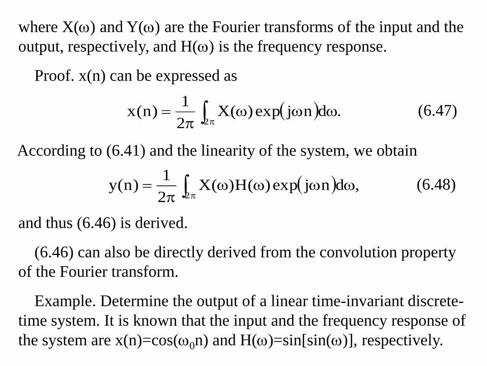
where X() and Y() are the Fourier transforms of the input and the

output, respectively, and H() is the frequency response.

Proof. x(n) can be expressed as

.dnjexp)(X2

1)n(x

2

(6.47)

According to (6.41) and the linearity of the system, we obtain

and thus (6.46) is derived.

(6.46) can also be directly derived from the convolution property

of the Fourier transform.

Example. Determine the output of a linear time-invariant discrete-

time system. It is known that the input and the frequency response of

the system are x(n)=cos(0n) and H()=sin[sin()], respectively.

,dnjexp)(H)(X2

1)n(y

2

(6.48)

Example. A distortionless transmission system is described by

y(n)=Ax(nn0). (6.49)

Find the frequency response.

Example. The frequency response can be expressed in terms of its

amplitude and phase, i.e.,

H()=|H()|ejH(). (6.50)

The minus derivative of H() is called the group delay. Show that

the group delay of a distortionless transmission system is a constant.

Example. The frequency response of an ideal low-pass filter is

(6.51)

over period [, ). Find the impulse response.

0

0

|| 0,

|| ,1)H(

Example. An ideal filter is best in frequency selectivity. However,

it is noncausal, and its impulse response is oscillatory. These defects

can be overcome by using a non-ideal filter. The frequency response

of a typical non-ideal low-pass filter is

,)jexp(a1

a1)(H

(6.52)

where 0<a<1. Find the impulse response.

Example. Two ideal low-pass filters have the frequency responses

(6.53)

and

(6.54)

1

1

1|| 0,

|| ,1)(H

2

2

2|| 0,

|| ,1)(H

over period [, ), respectively. 1+2< here. The two filters can

be used to construct an ideal band-stop filter, as shown in figure 6.3.

Explain how it works.

Figure 6.3. Implementation of a Band-Stop Filter.

6.7. Linear Constant-Coefficient Difference Equations

The zero-state response of a linear constant-coefficient difference

equation can be found using the Fourier transform.

x(n)

e(n) r(n)

y(n)

(1)n

H2()

(1)n

H1()

y2(n)

y1(n)

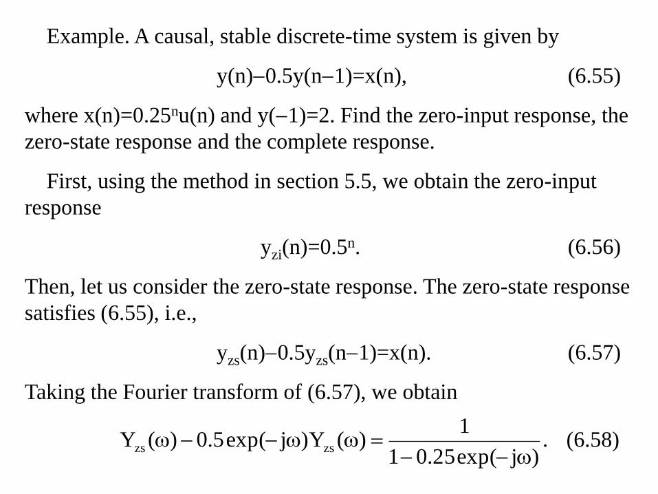
Example. A causal, stable discrete-time system is given by

y(n)0.5y(n1)=x(n), (6.55)

where x(n)=0.25nu(n) and y(1)=2. Find the zero-input response, the

zero-state response and the complete response.

First, using the method in section 5.5, we obtain the zero-input

response

yzi(n)=0.5n. (6.56)

Then, let us consider the zero-state response. The zero-state response

satisfies (6.55), i.e.,

yzs(n)0.5yzs(n1)=x(n). (6.57)

Taking the Fourier transform of (6.57), we obtain

.)jexp(25.01

1)(Y)jexp(5.0)(Y zszs

(6.58)

From (6.58), we obtain

.)jexp(25.01

1

)jexp(5.01

2)(Yzs

(6.59)

The inverse Fourier transform of Yzs() is

yzs(n)=(2·0.5n0.25n)u(n). (6.60)

The complete response is the sum of the zero-input response and the

zero-state response, i.e.,

y(n)=0.5n+(2·0.5n0.25n)u(n). (6.61)

Example. A stable discrete-time system is given by

y(n)0.5y(n1)=x(n). (6.62)

Find the impulse response.

The zero-state response satisfies (6.62), i.e.,

yzs(n)0.5yzs(n1)=x(n). (6.63)

Taking the Fourier transform of (6.63), we obtain

.)jexp(5.01

1

)(X

)(Yzs

(6.64)

Thus,

.)jexp(5.01

1)(H

(6.65)

The inverse Fourier transform of H() is

h(n)=0.5nu(n). (6.66)