Embed Size (px)
Citation preview
13
6 EMC403 Electrical Machine Design 7 MGT301 Entrepreneurship
Development
8 PSS407 Advanced Power System Protection
9 PSS408 Power Market and Trading
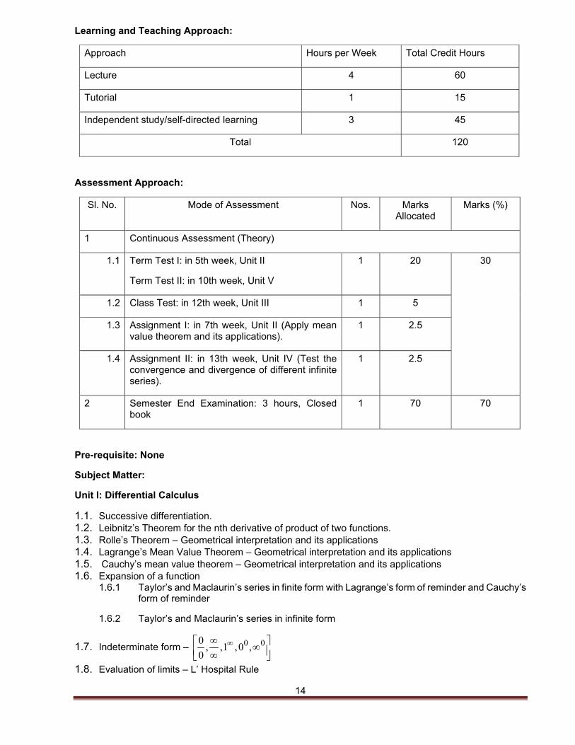
3. Module Descriptors
Semester I Contact Hours Credit
Marks
Theory Pract
# Code Module L T P CA EX CA 1 MAT101 Engineering Mathematics-I 4 1 0 12 30 70 0 2 PHY101 Engineering Physics-I 4 0 2 12 25 50 25 3 CHE101 Engineering Chemistry 3 1 2 12 25 50 25 4 CPL101 Introduction to Programming 3 1 2 12 25 50 25 5 EGP101 Engineering Graphics 1 0 6 12 50 50 0 Total contact hours/week = 30 hrs Total Marks=500
Module Code & Title : MAT101 Engineering Mathematics-I
Programme : BE in Civil Engineering
Credit : 12
Module Tutor : Mrs. Jyoti Lakshmi S and Ms. Tshering Denka
Module Coordinator : Mrs. Jyoti Lakshmi S
General Objectives:
To develop the student’s abilities in mathematics, in particular the concept of Differential Calculus, Integral Calculus and Differential Equation that finds applications in various fields of Engineering.
Learning Outcomes:
On completion of the module, students will be able to:
1. Differentiate successive function by applying Leibnitz’s theorem to find the nth derivative of the function by applying Leibnitz’s theorem.
2. Apply appropriate Mean Value Theorems to expand the given function. 3. Identify the indeterminate form and evaluate the Limits. 4. Use Partial Differentiation to find the Jacobians of functions of two or more variables and expand the
two variable functions by Taylor’s series. 5. Choose the appropriate application of partial differentiation to find the Maxima and Minima of functions
of two variables. 6. Employ Reduction formula to find the Integral and Definite Integral of functions. 7. Apply appropriate methods to test the Convergence and Divergence of different infinite series. 8. Solve Differential Equations of first order first degree and first order higher degree. 9. Find the Rank of a Matrix. 10. Solve Simultaneous Equation by Matrix method.
14
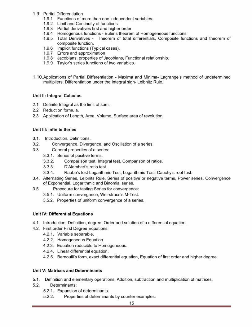
Learning and Teaching Approach:
Approach Hours per Week Total Credit Hours
Lecture 4 60
Tutorial 1 15
Independent study/self-directed learning 3 45
Total 120
Assessment Approach:
Sl. No. Mode of Assessment Nos. Marks Allocated
Marks (%)
1 Continuous Assessment (Theory)
1.1 Term Test I: in 5th week, Unit II
Term Test II: in 10th week, Unit V
1 20 30
1.2 Class Test: in 12th week, Unit III 1 5
1.3 Assignment I: in 7th week, Unit II (Apply mean value theorem and its applications).
1 2.5
1.4 Assignment II: in 13th week, Unit IV (Test the convergence and divergence of different infinite series).
1 2.5
2 Semester End Examination: 3 hours, Closed book
1 70 70
Pre-requisite: None
Subject Matter:
Unit I: Differential Calculus
1.1. Successive differentiation. 1.2. Leibnitz’s Theorem for the nth derivative of product of two functions. 1.3. Rolle’s Theorem – Geometrical interpretation and its applications 1.4. Lagrange’s Mean Value Theorem – Geometrical interpretation and its applications 1.5. Cauchy’s mean value theorem – Geometrical interpretation and its applications 1.6. Expansion of a function
1.6.1 Taylor’s and Maclaurin’s series in finite form with Lagrange’s form of reminder and Cauchy’s form of reminder
1.6.2 Taylor’s and Maclaurin’s series in infinite form
1.7. Indeterminate form – 0 00, ,1 ,0 ,
0
1.8. Evaluation of limits – L’ Hospital Rule
15
1.9. Partial Differentiation 1.9.1 Functions of more than one independent variables. 1.9.2 Limit and Continuity of functions 1.9.3 Partial derivatives first and higher order 1.9.4 Homogenous functions - Euler’s theorem of Homogeneous functions 1.9.5 Total Derivatives - Theorem of total differentials, Composite functions and theorem of
composite function, 1.9.6 Implicit functions (Typical cases), 1.9.7 Errors and approximation 1.9.8 Jacobians, properties of Jacobians, Functional relationship. 1.9.9 Taylor’s series functions of two variables.
1.10. Applications of Partial Differentiation - Maxima and Minima- Lagrange’s method of undetermined multipliers, Differentiation under the Integral sign- Leibnitz Rule.
Unit II: Integral Calculus
2.1 Definite Integral as the limit of sum. 2.2 Reduction formula. 2.3 Application of Length, Area, Volume, Surface area of revolution.
Unit III: Infinite Series
3.1. Introduction, Definitions. 3.2. Convergence, Divergence, and Oscillation of a series. 3.3. General properties of a series:
3.3.1. Series of positive terms. 3.3.2. Comparison test, Integral test, Comparison of ratios. 3.3.3. D’Alembert’s ratio test. 3.3.4. Raabe’s test Logarithmic Test, Logarithmic Test, Cauchy’s root test.
3.4. Alternating Series, Leibnits Rule, Series of positive or negative terms, Power series, Convergence of Exponential, Logarithmic and Binomial series.
3.5. Procedure for testing Series for convergence: 3.5.1. Uniform convergence, Weirstrass’s M-Test. 3.5.2. Properties of uniform convergence of a series.
Unit IV: Differential Equations
4.1. Introduction, Definition, degree, Order and solution of a differential equation. 4.2. First order First Degree Equations:
4.2.1. Variable separable. 4.2.2. Homogeneous Equation 4.2.3. Equation reducible to Homogeneous. 4.2.4. Linear differential equation. 4.2.5. Bernoulli’s form, exact differential equation, Equation of first order and higher degree.
Unit V: Matrices and Determinants
5.1. Definition and elementary operations, Addition, subtraction and multiplication of matrices. 5.2. Determinants:
5.2.1. Expansion of determinants. 5.2.2. Properties of determinants by counter examples.
16
5.2.3. Minors and co-factor of a determinant. 5.2.4. Determinant of a square Matrix. 5.2.5. Adjoin of a square matrix, Matrix inverse. 5.2.6. Solution of simultaneous equation by Matrix method. 5.2.7. Rank of a matrix, Elementary transformation of a matrix.
Reading Lists:
Essential reading:
1. Kreyszig, E. (2002). Advanced Engineering Mathematics (8 ed.). Singapore: John Wiley & Sons (Asia) Pvt Ltd.
2. Grewal, B.S. (2001). Higher Engineering Mathematics (36 ed). New Delhi: Khanna Publishers. 3. Dass, H.K. (2005). Advanced Engineering Mathematics (14 ed.). New Delhi: S.Chand& Company Ltd. 4. Jain, R. K., & Iyengar, R.K. (2003). Advanced Engineering Mathematics (2 ed.). New Delhi: Narosa
Publishing house. 5. Prasad, I. B. (1982). Practical Mathematics Vol I and Vol II (6 ed.). New Delhi: Khanna Publishers. Additional Reading:
1. Rao, S. B., & Anuradha, H. R. (1996). Differential Equations with Application and Programmes (1 ed.). Hyderabad: Universities Press (India) Ltd.
2. Vasishtha, A. R. (2002). Matrices (32 ed.). Meerut: Krishna Prakashan Media (P) Ltd. 3. Bali N.P &cDr. Manish Goyal (2014) A Text Book of Engineering Mathematics (9 ed). New Delhi :
Laxmi Publications(P) Ltd. 4. Babu Ram, (2010), Engineering Mathematics (1 ed). New Delhi : Pearson
Date: 04 Feb, 2017
17
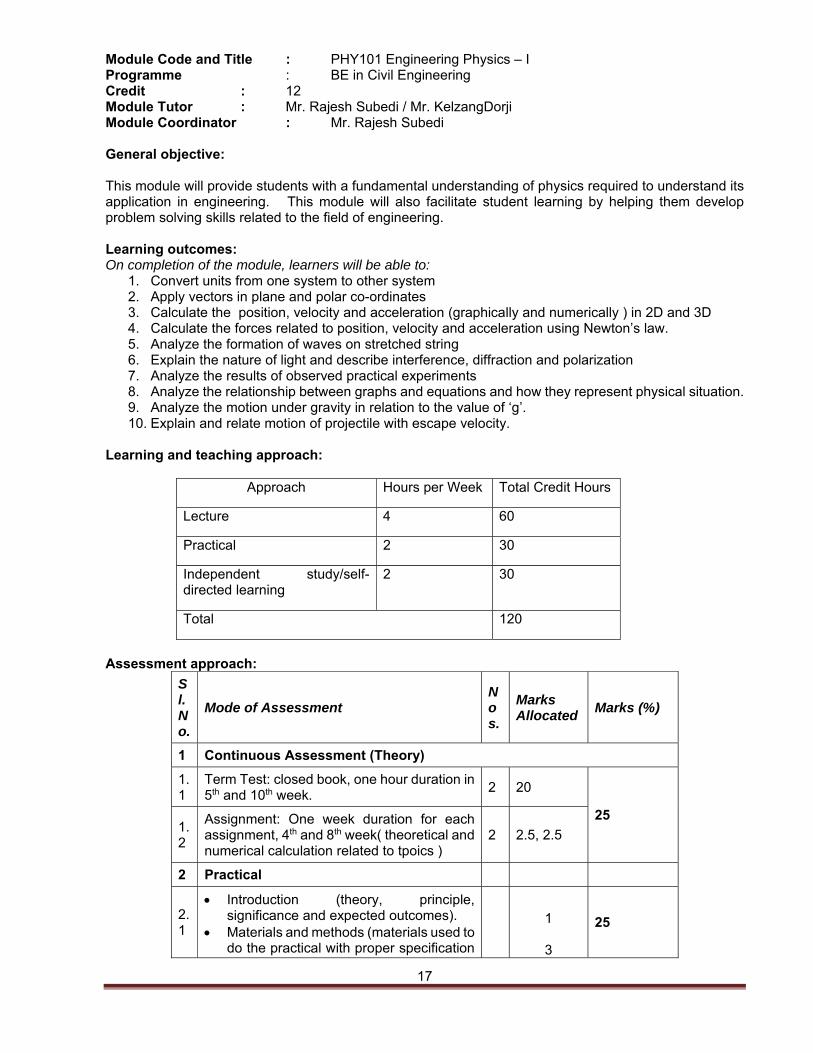
Module Code and Title : PHY101 Engineering Physics – I Programme : BE in Civil Engineering Credit : 12 Module Tutor : Mr. Rajesh Subedi / Mr. KelzangDorji Module Coordinator : Mr. Rajesh Subedi General objective: This module will provide students with a fundamental understanding of physics required to understand its application in engineering. This module will also facilitate student learning by helping them develop problem solving skills related to the field of engineering. Learning outcomes: On completion of the module, learners will be able to:
1. Convert units from one system to other system 2. Apply vectors in plane and polar co-ordinates 3. Calculate the position, velocity and acceleration (graphically and numerically ) in 2D and 3D 4. Calculate the forces related to position, velocity and acceleration using Newton’s law. 5. Analyze the formation of waves on stretched string 6. Explain the nature of light and describe interference, diffraction and polarization 7. Analyze the results of observed practical experiments 8. Analyze the relationship between graphs and equations and how they represent physical situation. 9. Analyze the motion under gravity in relation to the value of ‘g’. 10. Explain and relate motion of projectile with escape velocity.
Learning and teaching approach:
Approach Hours per Week Total Credit Hours
Lecture 4 60
Practical 2 30
Independent study/self-directed learning
2 30
Total 120
Assessment approach:
Sl. No.
Mode of Assessment Nos.
Marks Allocated
Marks (%)
1 Continuous Assessment (Theory)
1.1
Term Test: closed book, one hour duration in 5th and 10th week.
2 20
25 1.2
Assignment: One week duration for each assignment, 4th and 8th week( theoretical and numerical calculation related to tpoics )
2 2.5, 2.5
2 Practical
2.1
Introduction (theory, principle, significance and expected outcomes).
Materials and methods (materials used to do the practical with proper specification
1
3
25
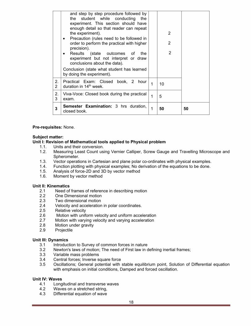
18
and step by step procedure followed by the student while conducting the experiment. This section should have enough detail so that reader can repeat the experiment).
Precaution (rules need to be followed in order to perform the practical with higher precision).
Results (state outcomes of the experiment but not interpret or draw conclusions about the data).
Conclusion (state what student has learned by doing the experiment).
2
2
2
2.2
Practical Exam: Closed book, 2 hour duration in 14th week.
1 10
2.3
Viva-Voce: Closed book during the practical exam.
1 5
3 Semester Examination: 3 hrs duration, closed book.
1 50 50
Pre-requisites: None. Subject matter: Unit I: Revision of Mathematical tools applied to Physical problem
1.1. Units and their conversion. 1.2. Measuring Least Count using Vernier Calliper, Screw Gauge and Travelling Microscope and
Spherometer. 1.3. Vector operations in Cartesian and plane polar co-ordinates with physical examples. 1.4. Function plotting with physical examples; No derivation of the equations to be done. 1.5. Analysis of force-2D and 3D by vector method 1.6. Moment by vector method
Unit II: Kinematics
2.1 Need of frames of reference in describing motion 2.2 One Dimensional motion 2.3 Two dimensional motion 2.4 Velocity and acceleration in polar coordinates. 2.5 Relative velocity 2.6 Motion with uniform velocity and uniform acceleration 2.7 Motion with varying velocity and varying acceleration 2.8 Motion under gravity 2.9 Projectile
Unit III: Dynamics
3.1 Introduction to Survey of common forces in nature 3.2 Newton's laws of motion; The need of First law in defining inertial frames; 3.3 Variable mass problems 3.4 Central forces; Inverse square force 3.5 Oscillations; General potential with stable equilibrium point, Solution of Differential equation
with emphasis on initial conditions, Damped and forced oscillation. Unit IV: Waves
4.1 Longitudinal and transverse waves 4.2 Waves on a stretched string, 4.3 Differential equation of wave
19
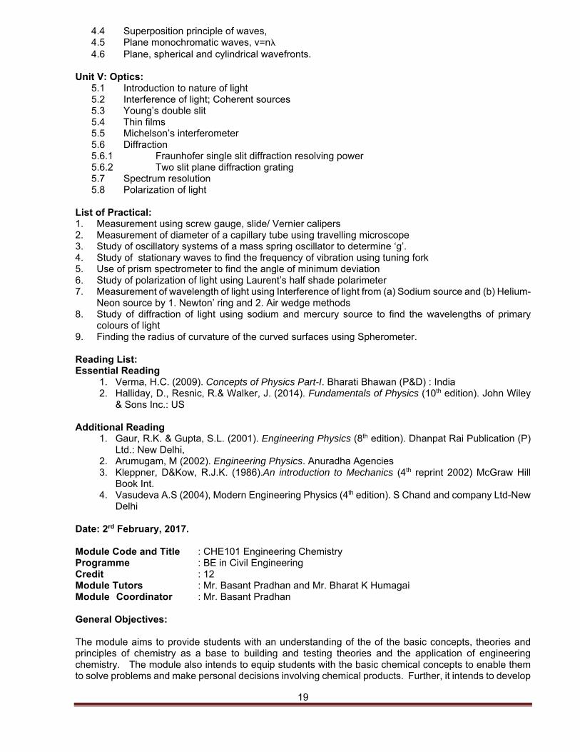
4.4 Superposition principle of waves, 4.5 Plane monochromatic waves, v=n 4.6 Plane, spherical and cylindrical wavefronts.
Unit V: Optics:
5.1 Introduction to nature of light 5.2 Interference of light; Coherent sources 5.3 Young’s double slit 5.4 Thin films 5.5 Michelson’s interferometer 5.6 Diffraction 5.6.1 Fraunhofer single slit diffraction resolving power 5.6.2 Two slit plane diffraction grating 5.7 Spectrum resolution 5.8 Polarization of light
List of Practical: 1. Measurement using screw gauge, slide/ Vernier calipers 2. Measurement of diameter of a capillary tube using travelling microscope 3. Study of oscillatory systems of a mass spring oscillator to determine ‘g’. 4. Study of stationary waves to find the frequency of vibration using tuning fork 5. Use of prism spectrometer to find the angle of minimum deviation 6. Study of polarization of light using Laurent’s half shade polarimeter 7. Measurement of wavelength of light using Interference of light from (a) Sodium source and (b) Helium-
Neon source by 1. Newton’ ring and 2. Air wedge methods 8. Study of diffraction of light using sodium and mercury source to find the wavelengths of primary
colours of light 9. Finding the radius of curvature of the curved surfaces using Spherometer. Reading List: Essential Reading
1. Verma, H.C. (2009). Concepts of Physics Part-I. Bharati Bhawan (P&D) : India 2. Halliday, D., Resnic, R.& Walker, J. (2014). Fundamentals of Physics (10th edition). John Wiley
& Sons Inc.: US Additional Reading
1. Gaur, R.K. & Gupta, S.L. (2001). Engineering Physics (8th edition). Dhanpat Rai Publication (P) Ltd.: New Delhi,
2. Arumugam, M (2002). Engineering Physics. Anuradha Agencies 3. Kleppner, D&Kow, R.J.K. (1986).An introduction to Mechanics (4th reprint 2002) McGraw Hill
Book Int. 4. Vasudeva A.S (2004), Modern Engineering Physics (4th edition). S Chand and company Ltd-New
Delhi Date: 2rd February, 2017. Module Code and Title : CHE101 Engineering Chemistry Programme : BE in Civil Engineering Credit : 12 Module Tutors : Mr. Basant Pradhan and Mr. Bharat K Humagai Module Coordinator : Mr. Basant Pradhan General Objectives: The module aims to provide students with an understanding of the of the basic concepts, theories and principles of chemistry as a base to building and testing theories and the application of engineering chemistry. The module also intends to equip students with the basic chemical concepts to enable them to solve problems and make personal decisions involving chemical products. Further, it intends to develop
20
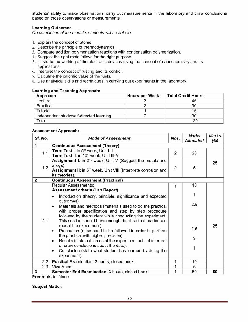
students’ ability to make observations, carry out measurements in the laboratory and draw conclusions based on those observations or measurements. Learning Outcomes On completion of the module, students will be able to: 1. Explain the concept of atoms. 2. Describe the principle of thermodynamics. 3. Compare addition polymerization reactions with condensation polymerization. 4. Suggest the right metal/alloys for the right purpose. 5. Illustrate the working of the electronic devices using the concept of nanochemistry and its
applications. 6. Interpret the concept of rusting and its control. 7. Calculate the calorific value of the fuels. 8. Use analytical skills and techniques in carrying out experiments in the laboratory.
Learning and Teaching Approach:
Approach Hours per Week Total Credit Hours Lecture 3 45 Practical 2 30 Tutorial 1 15 Independent study/self-directed learning 2 30 Total 120
Assessment Approach:
Prerequisite: None Subject Matter:
Sl. No. Mode of Assessment Nos. Marks
Allocated Marks
(%) 1 Continuous Assessment (Theory)
1.1 Term Test I: in 5th week, Unit I-II Term Test II: in 10th week, Unit III-V
2 20
25 1.2
Assignment I: in 2nd week, Unit V (Suggest the metals and alloys). Assignment II: in 5th week, Unit VIII (Interprete corrosion and its theories).
2 5
2 Continuous Assessment (Practical)
2.1
Regular Assessments: Assessment criteria (Lab Report)
Introduction (theory, principle, significance and expected outcomes).
Materials and methods (materials used to do the practical with proper specification and step by step procedure followed by the student while conducting the experiment. This section should have enough detail so that reader can repeat the experiment).
Precaution (rules need to be followed in order to perform the practical with higher precision).
Results (state outcomes of the experiment but not interpret or draw conclusions about the data).
Conclusion (state what student has learned by doing the experiment).
1 10
1
2.5
2.5
3
1
25
2.2 Practical Examination: 2 hours, closed book. 1 10 2.3 Viva-Voce: 1 5
3 Semester End Examination: 3 hours, closed book. 1 50 50
21
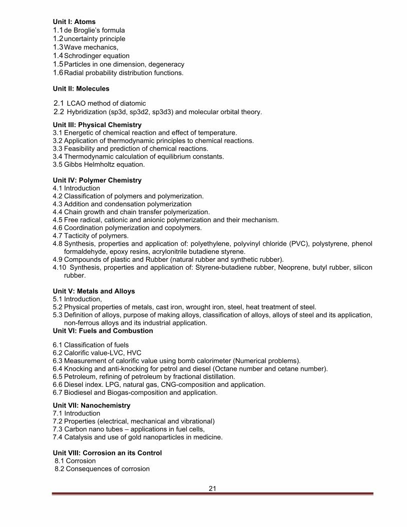
Unit I: Atoms 1.1 de Broglie’s formula 1.2 uncertainty principle 1.3 Wave mechanics, 1.4 Schrodinger equation 1.5 Particles in one dimension, degeneracy 1.6 Radial probability distribution functions. Unit II: Molecules
2.1 LCAO method of diatomic 2.2 Hybridization (sp3d, sp3d2, sp3d3) and molecular orbital theory.
Unit III: Physical Chemistry 3.1 Energetic of chemical reaction and effect of temperature. 3.2 Application of thermodynamic principles to chemical reactions. 3.3 Feasibility and prediction of chemical reactions. 3.4 Thermodynamic calculation of equilibrium constants. 3.5 Gibbs Helmholtz equation. Unit IV: Polymer Chemistry 4.1 Introduction 4.2 Classification of polymers and polymerization. 4.3 Addition and condensation polymerization 4.4 Chain growth and chain transfer polymerization. 4.5 Free radical, cationic and anionic polymerization and their mechanism. 4.6 Coordination polymerization and copolymers. 4.7 Tacticity of polymers. 4.8 Synthesis, properties and application of: polyethylene, polyvinyl chloride (PVC), polystyrene, phenol
formaldehyde, epoxy resins, acrylonitrile butadiene styrene. 4.9 Compounds of plastic and Rubber (natural rubber and synthetic rubber). 4.10 Synthesis, properties and application of: Styrene-butadiene rubber, Neoprene, butyl rubber, silicon
rubber. Unit V: Metals and Alloys 5.1 Introduction, 5.2 Physical properties of metals, cast iron, wrought iron, steel, heat treatment of steel. 5.3 Definition of alloys, purpose of making alloys, classification of alloys, alloys of steel and its application,
non-ferrous alloys and its industrial application. Unit VI: Fuels and Combustion
6.1 Classification of fuels 6.2 Calorific value-LVC, HVC 6.3 Measurement of calorific value using bomb calorimeter (Numerical problems). 6.4 Knocking and anti-knocking for petrol and diesel (Octane number and cetane number). 6.5 Petroleum, refining of petroleum by fractional distillation. 6.6 Diesel index. LPG, natural gas, CNG-composition and application. 6.7 Biodiesel and Biogas-composition and application.
Unit VII: Nanochemistry 7.1 Introduction 7.2 Properties (electrical, mechanical and vibrational) 7.3 Carbon nano tubes – applications in fuel cells, 7.4 Catalysis and use of gold nanoparticles in medicine. Unit VIII: Corrosion an its Control 8.1 Corrosion 8.2 Consequences of corrosion
22
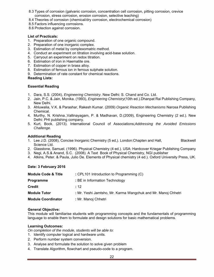
8.3 Types of corrosion (galvanic corrosion, concentration cell corrosion, pitting corrosion, crevice corrosion, stress corrosion, erosion corrosion, selective leaching)
8.4 Theories of corrosion (chemical/dry corrosion, electrochemical corrosion) 8.5 Factors influencing corrosions. 8.6 Protection against corrosion. List of Practicals: 1. Preparation of one organic compound. 2. Preparation of one inorganic complex. 3. Estimation of metal by complexomatric method. 4. Conduct an experiment on titration involving acid-base solution. 5. Carryout an experiment on redox titration. 6. Estimation of iron in Haematite ore. 7. Estimation of copper in brass alloy. 8. Estimation of ferrous ion in ferrous sulphate solution. 9. Determination of rate constant for chemical reactions. Reading Lists: Essential Reading 1. Dara, S.S. (2004), Engineering Chemistry. New Delhi: S. Chand and Co. Ltd. 2. Jain, P.C. & Jain, Monika. (1993), Engineering Chemistry(10th ed.).Dhanpat Rai Publishing Company,
New Delhi. 3. Ahluwalia, V.K. & Parashar, Rakesh Kumar. (2009) Organic Reaction Mechanisms Narosa Publishing
Chemical. 4. Murthy, N. Krishna.,Vallinayagam, P. & Madhavan, D.(2009), Engineering Chemistry (2 ed.). New
Delhi: PHI publishing company. 5. Kurt, Bock. (2013). International Council of Associations;Addressing the Avoided Emissions
Challenge. ,
Additional Reading 1. Lee J.D. (2008), Concise Inorganic Chemistry (5 ed,). London:Chapten and Hall, Blackwell
Science Ltd. 2. Glasstone, Samuel. (1996). Physical Chemistry (4 ed.). USA: Hardcover Kriegar Publishing Company 3. Negi, A.S.& Anand, S.C. (2008). A Text Book of Physical Chemistry, NGI publisher 4. Atkins, Peter. & Paula, Julio De. Elements of Physical chemistry (4 ed.). Oxford University Press, UK.
Date: 3 February 2016
Module Code & Title : CPL101 Introduction to Programming (C)
Programme : BE in Information Technology
Credit : 12
Module Tutor : Mr. Yeshi Jamtsho, Mr. Karma Wangchuk and Mr. Manoj Chhetri
Module Coordinator : Mr. Manoj Chhetri
General Objective: This module will familiarise students with programming concepts and the fundamentals of programming language to enable them to formulate and design solutions for basic mathematical problems. Learning Outcomes: On completion of the module, students will be able to: 1. Identify computer logical and hardware units. 2. Perform number system conversion. 3. Analyse and formulate the solution to solve given problem 4. Translate Algorithm, flowchart and pseudo-code to a program.
23
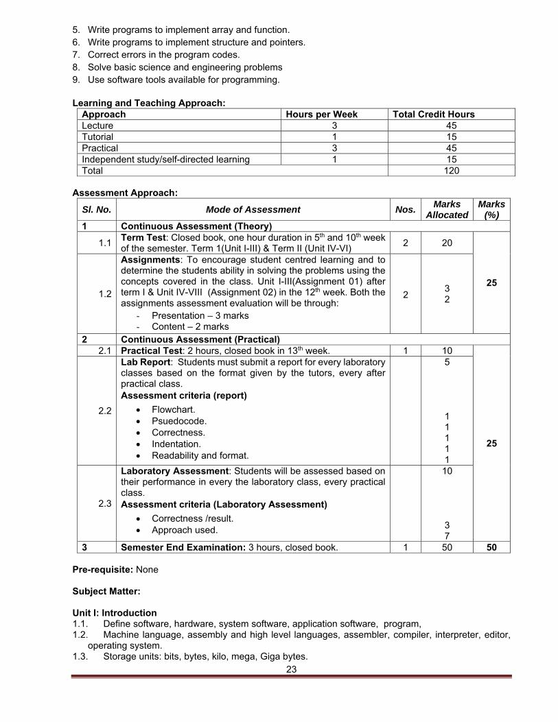
5. Write programs to implement array and function. 6. Write programs to implement structure and pointers. 7. Correct errors in the program codes. 8. Solve basic science and engineering problems 9. Use software tools available for programming. Learning and Teaching Approach:
Approach Hours per Week Total Credit HoursLecture 3 45 Tutorial 1 15 Practical 3 45 Independent study/self-directed learning 1 15 Total 120
Assessment Approach:
Sl. No. Mode of Assessment Nos. Marks
AllocatedMarks
(%) 1 Continuous Assessment (Theory)
1.1 Term Test: Closed book, one hour duration in 5th and 10th week of the semester. Term 1(Unit I-III) & Term II (Unit IV-VI)
2 20
25 1.2
Assignments: To encourage student centred learning and to determine the students ability in solving the problems using the concepts covered in the class. Unit I-III(Assignment 01) after term I & Unit IV-VIII (Assignment 02) in the 12th week. Both the assignments assessment evaluation will be through:
- Presentation – 3 marks - Content – 2 marks
2 3 2
2 Continuous Assessment (Practical) 2.1 Practical Test: 2 hours, closed book in 13th week. 1 10
25
2.2
Lab Report: Students must submit a report for every laboratory classes based on the format given by the tutors, every after practical class. Assessment criteria (report)
Flowchart. Psuedocode. Correctness. Indentation. Readability and format.
5
1 1 1 1 1
2.3
Laboratory Assessment: Students will be assessed based on their performance in every the laboratory class, every practical class. Assessment criteria (Laboratory Assessment)
Correctness /result. Approach used.
10
3 7
3 Semester End Examination: 3 hours, closed book. 1 50 50 Pre-requisite: None Subject Matter: Unit I: Introduction 1.1. Define software, hardware, system software, application software, program, 1.2. Machine language, assembly and high level languages, assembler, compiler, interpreter, editor,
operating system. 1.3. Storage units: bits, bytes, kilo, mega, Giga bytes.
24
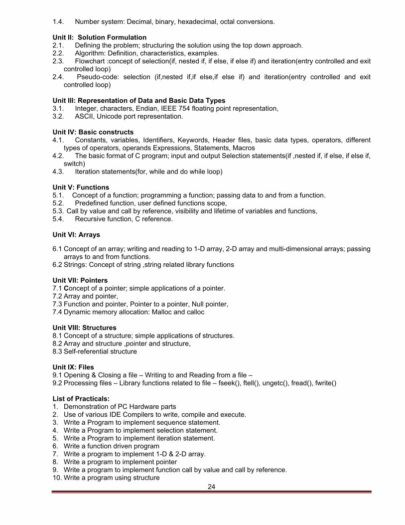
1.4. Number system: Decimal, binary, hexadecimal, octal conversions.
Unit II: Solution Formulation 2.1. Defining the problem; structuring the solution using the top down approach. 2.2. Algorithm: Definition, characteristics, examples. 2.3. Flowchart :concept of selection(if, nested if, if else, if else if) and iteration(entry controlled and exit
controlled loop) 2.4. Pseudo-code: selection (if,nested if,if else,if else if) and iteration(entry controlled and exit
controlled loop) Unit III: Representation of Data and Basic Data Types 3.1. Integer, characters, Endian, IEEE 754 floating point representation, 3.2. ASCII, Unicode port representation.
Unit IV: Basic constructs 4.1. Constants, variables, Identifiers, Keywords, Header files, basic data types, operators, different
types of operators, operands Expressions, Statements, Macros 4.2. The basic format of C program; input and output Selection statements(if ,nested if, if else, if else if,
switch) 4.3. Iteration statements(for, while and do while loop) Unit V: Functions 5.1. Concept of a function; programming a function; passing data to and from a function. 5.2. Predefined function, user defined functions scope, 5.3. Call by value and call by reference, visibility and lifetime of variables and functions, 5.4. Recursive function, C reference.
Unit VI: Arrays
6.1 Concept of an array; writing and reading to 1-D array, 2-D array and multi-dimensional arrays; passing arrays to and from functions.
6.2 Strings: Concept of string ,string related library functions
Unit VII: Pointers 7.1 Concept of a pointer; simple applications of a pointer. 7.2 Array and pointer, 7.3 Function and pointer, Pointer to a pointer, Null pointer, 7.4 Dynamic memory allocation: Malloc and calloc Unit VIII: Structures 8.1 Concept of a structure; simple applications of structures. 8.2 Array and structure ,pointer and structure, 8.3 Self-referential structure Unit IX: Files 9.1 Opening & Closing a file – Writing to and Reading from a file – 9.2 Processing files – Library functions related to file – fseek(), ftell(), ungetc(), fread(), fwrite()
List of Practicals: 1. Demonstration of PC Hardware parts 2. Use of various IDE Compilers to write, compile and execute. 3. Write a Program to implement sequence statement. 4. Write a Program to implement selection statement. 5. Write a Program to implement iteration statement. 6. Write a function driven program 7. Write a program to implement 1-D & 2-D array. 8. Write a program to implement pointer 9. Write a program to implement function call by value and call by reference. 10. Write a program using structure
25
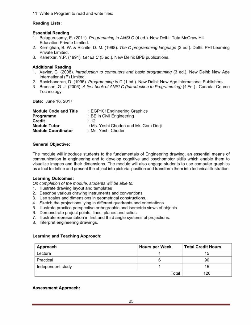
11. Write a Program to read and write files.
Reading Lists: Essential Reading 1. Balagurusamy, E. (2011). Programming in ANSI C (4 ed.). New Delhi: Tata McGraw Hill Education Private Limited. 2. Kernighan, B. W. & Richite, D. M. (1998). The C programming language (2 ed.). Delhi: PHI Learning
Private Limited. 3. Kanetkar, Y.P. (1991). Let us C (5 ed.). New Delhi: BPB publications.
Additional Reading 1. Xavier, C. (2008). Introduction to computers and basic programming (3 ed.). New Delhi: New Age
International (P) Limited. 2. Ravichandran, D. (1996). Programming in C (1 ed.). New Delhi: New Age international Publishers. 3. Bronson, G. J. (2006). A first book of ANSI C (Introduction to Programming) (4 Ed.). Canada: Course
Technology. Date: June 16, 2017 Module Code and Title : EGP101Engineering Graphics Programme : BE in Civil Engineering Credit : 12 Module Tutor : Ms. Yeshi Choden and Mr. Gom Dorji Module Coordinator : Ms. Yeshi Choden
General Objective: The module will introduce students to the fundamentals of Engineering drawing, an essential means of communication in engineering and to develop cognitive and psychomotor skills which enable them to visualize images and their dimensions. The module will also engage students to use computer graphics as a tool to define and present the object into pictorial position and transform them into technical illustration. Learning Outcomes: On completion of the module, students will be able to: 1. Illustrate drawing layout and templates 2. Describe various drawing instruments and conventions 3. Use scales and dimensions in geometrical constructions. 4. Sketch the projections lying in different quadrants and orientations. 5. Illustrate practice perspective orthographic and isometric views of objects. 6. Demonstrate project points, lines, planes and solids. 7. Illustrate representation in first and third angle systems of projections. 8. Interpret engineering drawings.
Learning and Teaching Approach:
Approach Hours per Week Total Credit Hours
Lecture 1 15
Practical 6 90
Independent study 1 15
Total 120
Assessment Approach:
26
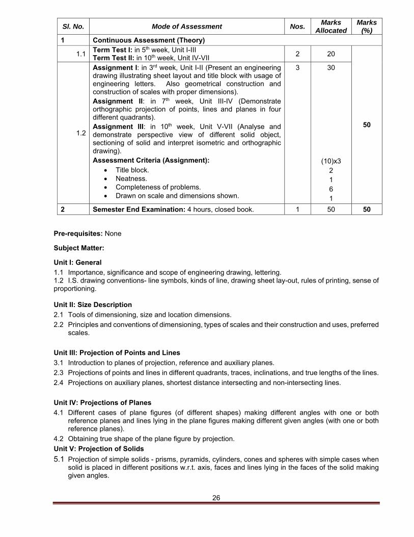
Sl. No. Mode of Assessment Nos. Marks
Allocated Marks
(%) 1 Continuous Assessment (Theory)
1.1 Term Test I: in 5th week, Unit I-III Term Test II: in 10th week, Unit IV-VII
2 20
50 1.2
Assignment I: in 3rd week, Unit I-II (Present an engineering drawing illustrating sheet layout and title block with usage of engineering letters. Also geometrical construction and construction of scales with proper dimensions). Assignment II: in 7th week, Unit III-IV (Demonstrate orthographic projection of points, lines and planes in four different quadrants). Assignment III: in 10th week, Unit V-VII (Analyse and demonstrate perspective view of different solid object, sectioning of solid and interpret isometric and orthographic drawing). Assessment Criteria (Assignment):
Title block. Neatness. Completeness of problems. Drawn on scale and dimensions shown.
3 30
(10)x3 2 1 6 1
2 Semester End Examination: 4 hours, closed book. 1 50 50
Pre-requisites: None
Subject Matter:
Unit I: General
1.1 Importance, significance and scope of engineering drawing, lettering. 1.2 I.S. drawing conventions- line symbols, kinds of line, drawing sheet lay-out, rules of printing, sense of proportioning.
Unit II: Size Description
2.1 Tools of dimensioning, size and location dimensions.
2.2 Principles and conventions of dimensioning, types of scales and their construction and uses, preferred scales.
Unit III: Projection of Points and Lines
3.1 Introduction to planes of projection, reference and auxiliary planes.
2.3 Projections of points and lines in different quadrants, traces, inclinations, and true lengths of the lines.
2.4 Projections on auxiliary planes, shortest distance intersecting and non-intersecting lines.
Unit IV: Projections of Planes
4.1 Different cases of plane figures (of different shapes) making different angles with one or both reference planes and lines lying in the plane figures making different given angles (with one or both reference planes).
4.2 Obtaining true shape of the plane figure by projection.
Unit V: Projection of Solids
5.1 Projection of simple solids - prisms, pyramids, cylinders, cones and spheres with simple cases when solid is placed in different positions w.r.t. axis, faces and lines lying in the faces of the solid making given angles.
27
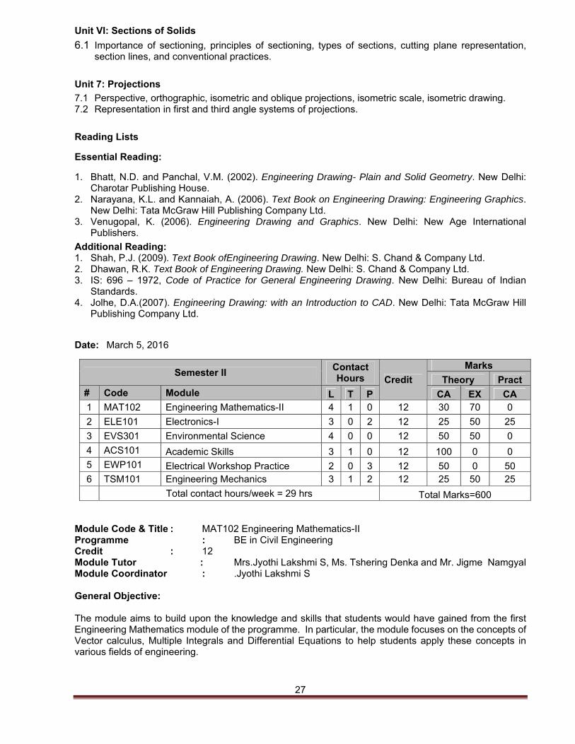
Unit VI: Sections of Solids
6.1 Importance of sectioning, principles of sectioning, types of sections, cutting plane representation, section lines, and conventional practices.
Unit 7: Projections
7.1 Perspective, orthographic, isometric and oblique projections, isometric scale, isometric drawing. 7.2 Representation in first and third angle systems of projections.
Reading Lists
Essential Reading:
1. Bhatt, N.D. and Panchal, V.M. (2002). Engineering Drawing- Plain and Solid Geometry. New Delhi: Charotar Publishing House.
2. Narayana, K.L. and Kannaiah, A. (2006). Text Book on Engineering Drawing: Engineering Graphics. New Delhi: Tata McGraw Hill Publishing Company Ltd.
3. Venugopal, K. (2006). Engineering Drawing and Graphics. New Delhi: New Age International Publishers.
Additional Reading: 1. Shah, P.J. (2009). Text Book ofEngineering Drawing. New Delhi: S. Chand & Company Ltd. 2. Dhawan, R.K. Text Book of Engineering Drawing. New Delhi: S. Chand & Company Ltd. 3. IS: 696 – 1972, Code of Practice for General Engineering Drawing. New Delhi: Bureau of Indian
Standards. 4. Jolhe, D.A.(2007). Engineering Drawing: with an Introduction to CAD. New Delhi: Tata McGraw Hill
Publishing Company Ltd.
Date: March 5, 2016
Semester II Contact Hours Credit
Marks
Theory Pract # Code Module L T P CA EX CA 1 MAT102 Engineering Mathematics-II 4 1 0 12 30 70 0
2 ELE101 Electronics-I 3 0 2 12 25 50 25
3 EVS301 Environmental Science 4 0 0 12 50 50 0
4 ACS101 Academic Skills 3 1 0 12 100 0 0 5 EWP101 Electrical Workshop Practice 2 0 3 12 50 0 50 6 TSM101 Engineering Mechanics 3 1 2 12 25 50 25
Total contact hours/week = 29 hrs Total Marks=600 Module Code & Title : MAT102 Engineering Mathematics-II Programme : BE in Civil Engineering Credit : 12 Module Tutor : Mrs.Jyothi Lakshmi S, Ms. Tshering Denka and Mr. Jigme Namgyal Module Coordinator : .Jyothi Lakshmi S General Objective: The module aims to build upon the knowledge and skills that students would have gained from the first Engineering Mathematics module of the programme. In particular, the module focuses on the concepts of Vector calculus, Multiple Integrals and Differential Equations to help students apply these concepts in various fields of engineering.
28
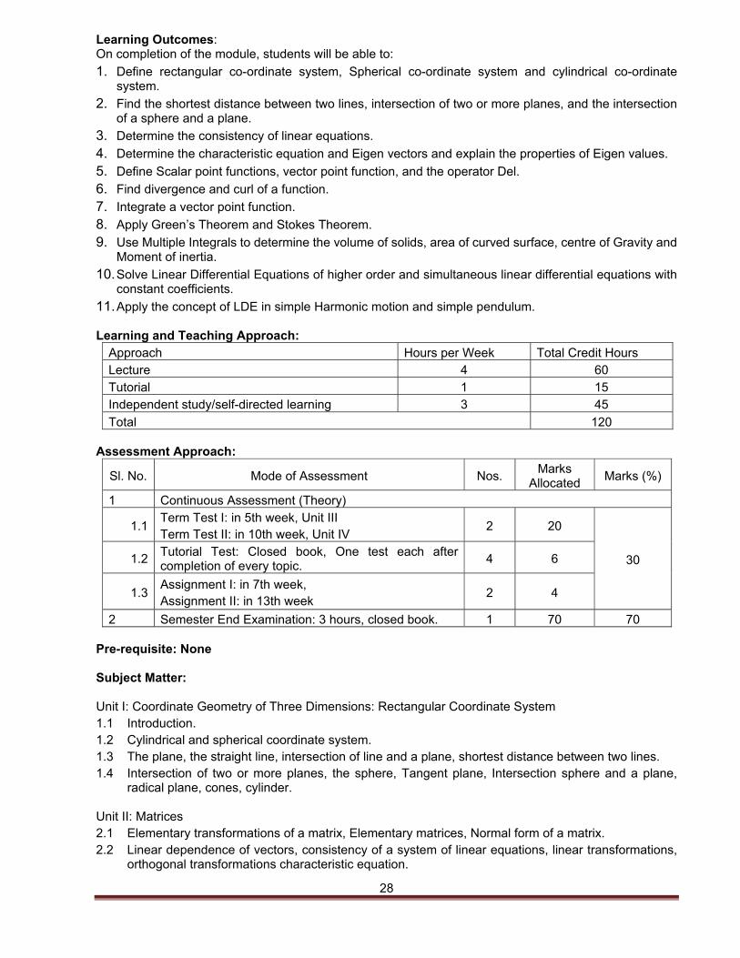
Learning Outcomes: On completion of the module, students will be able to:
1. Define rectangular co-ordinate system, Spherical co-ordinate system and cylindrical co-ordinate system.
2. Find the shortest distance between two lines, intersection of two or more planes, and the intersection of a sphere and a plane.
3. Determine the consistency of linear equations.
4. Determine the characteristic equation and Eigen vectors and explain the properties of Eigen values.
5. Define Scalar point functions, vector point function, and the operator Del.
6. Find divergence and curl of a function.
7. Integrate a vector point function.
8. Apply Green’s Theorem and Stokes Theorem.
9. Use Multiple Integrals to determine the volume of solids, area of curved surface, centre of Gravity and Moment of inertia.
10. Solve Linear Differential Equations of higher order and simultaneous linear differential equations with constant coefficients.
11. Apply the concept of LDE in simple Harmonic motion and simple pendulum.
Learning and Teaching Approach: Approach Hours per Week Total Credit HoursLecture 4 60 Tutorial 1 15Independent study/self-directed learning 3 45
Total 120 Assessment Approach:
Sl. No. Mode of Assessment Nos. Marks
Allocated Marks (%)
1 Continuous Assessment (Theory)
1.1 Term Test I: in 5th week, Unit III Term Test II: in 10th week, Unit IV
2 20
30 1.2 Tutorial Test: Closed book, One test each after completion of every topic.
4 6
1.3 Assignment I: in 7th week, Assignment II: in 13th week
2 4
2 Semester End Examination: 3 hours, closed book. 1 70 70 Pre-requisite: None Subject Matter: Unit I: Coordinate Geometry of Three Dimensions: Rectangular Coordinate System 1.1 Introduction. 1.2 Cylindrical and spherical coordinate system. 1.3 The plane, the straight line, intersection of line and a plane, shortest distance between two lines. 1.4 Intersection of two or more planes, the sphere, Tangent plane, Intersection sphere and a plane,
radical plane, cones, cylinder. Unit II: Matrices 2.1 Elementary transformations of a matrix, Elementary matrices, Normal form of a matrix. 2.2 Linear dependence of vectors, consistency of a system of linear equations, linear transformations,
orthogonal transformations characteristic equation.
29
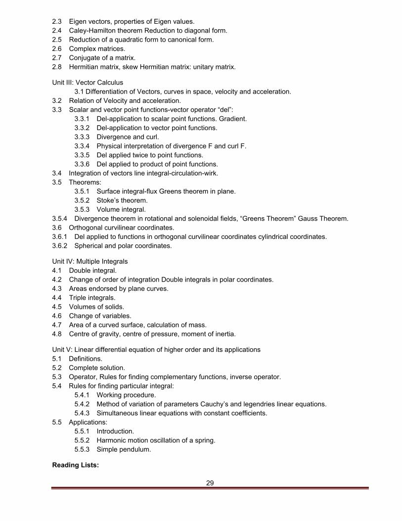
2.3 Eigen vectors, properties of Eigen values. 2.4 Caley-Hamilton theorem Reduction to diagonal form. 2.5 Reduction of a quadratic form to canonical form. 2.6 Complex matrices. 2.7 Conjugate of a matrix. 2.8 Hermitian matrix, skew Hermitian matrix: unitary matrix. Unit III: Vector Calculus
3.1 Differentiation of Vectors, curves in space, velocity and acceleration. 3.2 Relation of Velocity and acceleration. 3.3 Scalar and vector point functions-vector operator “del”:
3.3.1 Del-application to scalar point functions. Gradient. 3.3.2 Del-application to vector point functions. 3.3.3 Divergence and curl. 3.3.4 Physical interpretation of divergence F and curl F. 3.3.5 Del applied twice to point functions. 3.3.6 Del applied to product of point functions.
3.4 Integration of vectors line integral-circulation-wirk. 3.5 Theorems:
3.5.1 Surface integral-flux Greens theorem in plane. 3.5.2 Stoke’s theorem. 3.5.3 Volume integral.
3.5.4 Divergence theorem in rotational and solenoidal fields, “Greens Theorem” Gauss Theorem. 3.6 Orthogonal curvilinear coordinates. 3.6.1 Del applied to functions in orthogonal curvilinear coordinates cylindrical coordinates. 3.6.2 Spherical and polar coordinates. Unit IV: Multiple Integrals 4.1 Double integral. 4.2 Change of order of integration Double integrals in polar coordinates. 4.3 Areas endorsed by plane curves. 4.4 Triple integrals. 4.5 Volumes of solids. 4.6 Change of variables. 4.7 Area of a curved surface, calculation of mass. 4.8 Centre of gravity, centre of pressure, moment of inertia. Unit V: Linear differential equation of higher order and its applications 5.1 Definitions. 5.2 Complete solution. 5.3 Operator, Rules for finding complementary functions, inverse operator. 5.4 Rules for finding particular integral:
5.4.1 Working procedure. 5.4.2 Method of variation of parameters Cauchy’s and legendries linear equations. 5.4.3 Simultaneous linear equations with constant coefficients.
5.5 Applications: 5.5.1 Introduction. 5.5.2 Harmonic motion oscillation of a spring. 5.5.3 Simple pendulum.
Reading Lists:
30
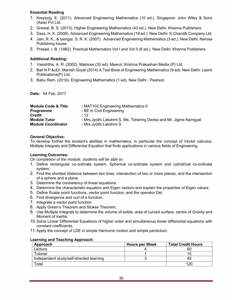
Essential Reading
1. Kreyszig, E. (2011). Advanced Engineering Mathematics (10 ed.). Singapore: John Wiley & Sons (Asia) Pvt Ltd.
2. Grewal, B. S. (2013). Higher Engineering Mathematics (43 ed.). New Delhi: Khanna Publishers.
3. Dass, H. K. (2008). Advanced Engineering Mathematics (19 ed.). New Delhi: S.Chand& Company Ltd.
4. Jain, R. K., & Iyengar, S. R. K. (2007). Advanced Engineering Mathematics (3 ed.). New Delhi: Narosa Publishing house.
5. Prasad, I. B. (1982). Practical Mathematics Vol I and Vol II (6 ed.). New Delhi: Khanna Publishers.
Additional Reading:
1. Vasishtha, A. R. (2002). Matrices (32 ed). Meerut: Krishna Prakashan Media (P) Ltd.
2. Bali N.P &cDr. Manish Goyal (2014) A Text Book of Engineering Mathematics (9 ed). New Delhi: Laxmi Publications(P) Ltd.
3. Babu Ram, (2010), Engineering Mathematics (1 ed). New Delhi : Pearson
Date: 04 Feb, 2017
Module Code & Title : MAT102 Engineering Mathematics-II Programme : BE in Civil Engineering Credit : 12 Module Tutor : Mrs.Jyothi Lakshmi S, Ms. Tshering Denka and Mr. Jigme Namgyal Module Coordinator : Mrs.Jyothi Lakshmi S
General Objective: To develop further the student’s abilities in mathematics, in particular the concept of Vector calculus, Multiple Integrals and Differential Equation that finds applications in various fields of Engineering. Learning Outcomes: On completion of the module, students will be able to: 1. Define rectangular co-ordinate system, Spherical co-ordinate system and cylindrical co-ordinate
system. 2. Find the shortest distance between two lines, intersection of two or more planes, and the intersection
of a sphere and a plane. 3. Determine the consistency of linear equations. 4. Determine the characteristic equation and Eigen vectors and explain the properties of Eigen values. 5. Define Scalar point functions, vector point function, and the operator Del. 6. Find divergence and curl of a function. 7. Integrate a vector point function. 8. Apply Green’s Theorem and Stokes Theorem. 9. Use Multiple Integrals to determine the volume of solids, area of curved surface, centre of Gravity and
Moment of inertia. 10. Solve Linear Differential Equations of higher order and simultaneous linear differential equations with
constant coefficients. 11. Apply the concept of LDE in simple Harmonic motion and simple pendulum. Learning and Teaching Approach:
Approach Hours per Week Total Credit Hours Lecture 4 60 Tutorial 1 15 Independent study/self-directed learning 3 45
Total 120
31
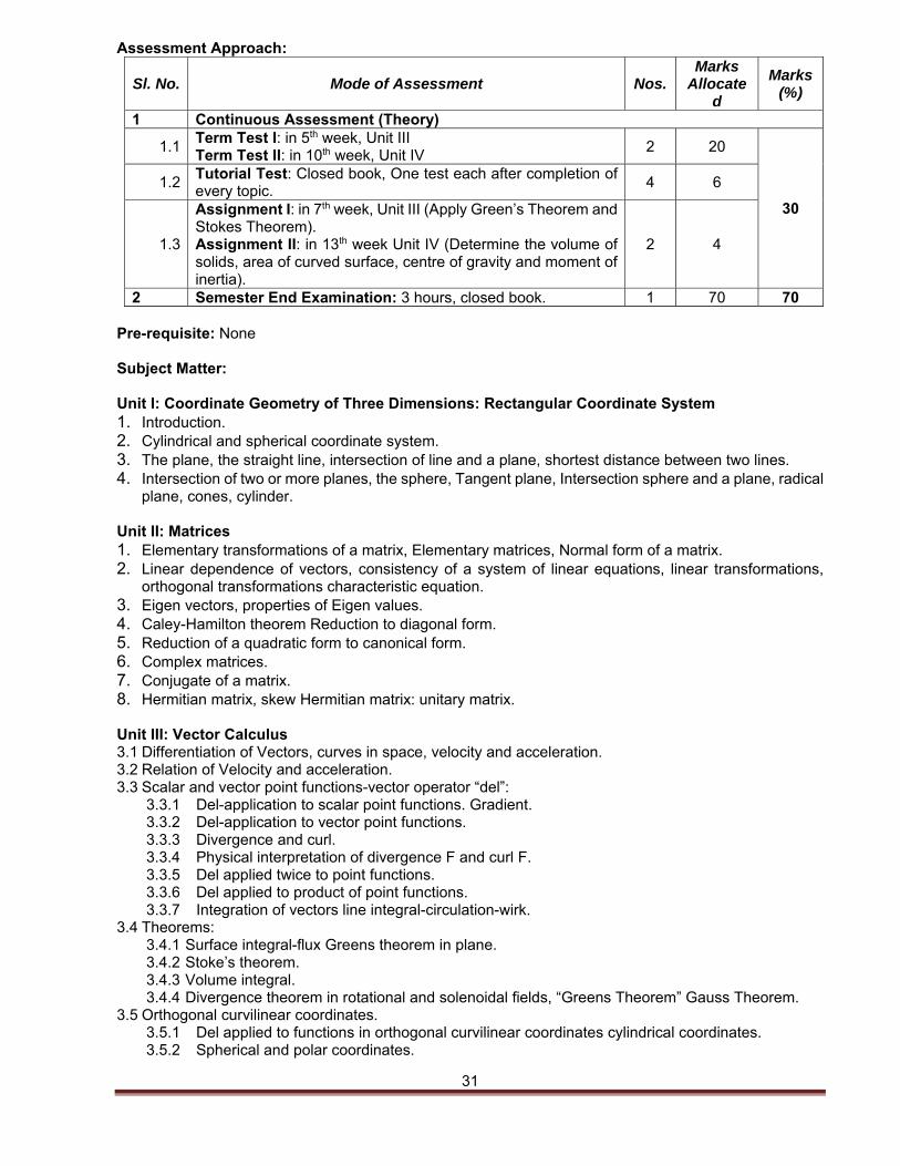
Assessment Approach:
Sl. No. Mode of Assessment Nos. Marks
Allocated
Marks (%)
1 Continuous Assessment (Theory)
1.1 Term Test I: in 5th week, Unit III Term Test II: in 10th week, Unit IV
2 20
30
1.2 Tutorial Test: Closed book, One test each after completion of every topic.
4 6
1.3
Assignment I: in 7th week, Unit III (Apply Green’s Theorem and Stokes Theorem). Assignment II: in 13th week Unit IV (Determine the volume of solids, area of curved surface, centre of gravity and moment of inertia).
2 4
2 Semester End Examination: 3 hours, closed book. 1 70 70 Pre-requisite: None Subject Matter: Unit I: Coordinate Geometry of Three Dimensions: Rectangular Coordinate System 1. Introduction. 2. Cylindrical and spherical coordinate system. 3. The plane, the straight line, intersection of line and a plane, shortest distance between two lines. 4. Intersection of two or more planes, the sphere, Tangent plane, Intersection sphere and a plane, radical
plane, cones, cylinder.
Unit II: Matrices 1. Elementary transformations of a matrix, Elementary matrices, Normal form of a matrix. 2. Linear dependence of vectors, consistency of a system of linear equations, linear transformations,
orthogonal transformations characteristic equation. 3. Eigen vectors, properties of Eigen values. 4. Caley-Hamilton theorem Reduction to diagonal form. 5. Reduction of a quadratic form to canonical form. 6. Complex matrices. 7. Conjugate of a matrix. 8. Hermitian matrix, skew Hermitian matrix: unitary matrix. Unit III: Vector Calculus 3.1 Differentiation of Vectors, curves in space, velocity and acceleration. 3.2 Relation of Velocity and acceleration. 3.3 Scalar and vector point functions-vector operator “del”:
3.3.1 Del-application to scalar point functions. Gradient. 3.3.2 Del-application to vector point functions. 3.3.3 Divergence and curl. 3.3.4 Physical interpretation of divergence F and curl F. 3.3.5 Del applied twice to point functions. 3.3.6 Del applied to product of point functions. 3.3.7 Integration of vectors line integral-circulation-wirk.
3.4 Theorems: 3.4.1 Surface integral-flux Greens theorem in plane. 3.4.2 Stoke’s theorem. 3.4.3 Volume integral. 3.4.4 Divergence theorem in rotational and solenoidal fields, “Greens Theorem” Gauss Theorem.
3.5 Orthogonal curvilinear coordinates. 3.5.1 Del applied to functions in orthogonal curvilinear coordinates cylindrical coordinates. 3.5.2 Spherical and polar coordinates.
32
Unit IV: Multiple Integrals
4.1 Double integral. 4.2 Change of order of integration Double integrals in polar coordinates. 4.3 Areas endorsed by plane curves. 4.4 Triple integrals. 4.5 Volumes of solids. 4.6 Change of variables 4.7 Area of a curved surface, calculation of mass 4.8 Centre of gravity, centre of pressure, moment of inertia.
Unit V: Linear differential equation of higher order and its applications 5.1 Definition 5.2 Complete solution. 5.3 Operator, Rules for finding complementary functions, inverse operator. 5.4 Rules for finding particular integral:
5.4.4 Working procedure. 5.4.5 Method of variation of parameters Cauchy’s and legendries linear equations. 5.4.6 Simultaneous linear equations with constant coefficients.
5.5 Applications: 5.5.4 Introduction. 5.5.5 Harmonic motion oscillation of a spring. 5.5.6 Simple pendulum.
Reading Lists:
Essential Reading 6. Kreyszig, E. (2011). Advanced Engineering Mathematics (10 ed.). Singapore: John Wiley & Sons
(Asia) Pvt Ltd. 7. Grewal, B. S. (2013). Higher Engineering Mathematics (43 ed.). New Delhi: Khanna Publishers. 8. Dass, H. K. (2008). Advanced Engineering Mathematics (19 ed.). New Delhi: S.Chand & Company
Ltd. Additional Reading: 4. Jain, R. K., & Iyengar, S. R. K. (2007). Advanced Engineering Mathematics (3 ed.). New Delhi: Narosa
Publishing house. 5. Prasad, I. B. (1982). Practical Mathematics Vol I and Vol II (6 ed.). New Delhi: Khanna Publishers. 6. Vasishtha, A. R. (2002). Matrices (32 ed). Meerut: Krishna Prakashan Media (P) Ltd. Date: 4th February 2017
33
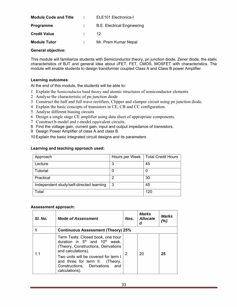
Module Code and Title : ELE101 Electronics-I
Programme : B.E. Electrical Engineering
Credit Value : 12
Module Tutor : Mr. Prem Kumar Nepal
General objective:
This module will familiarize students with Semiconductor theory, pn junction diode, Zener diode, the static characteristics of BJT and general idea about JFET, FET, CMOS, MOSFET with characteristics. The module will enable students to design transformer coupled Class A and Class B power Amplifier.
Learning outcomes:
At the end of this module, the students will be able to:
1 Explain the Semiconductor band theory and atomic structures of semiconductor elements 2 Analyse the characteristic of pn junction diode 3 Construct the half and full wave rectifiers, Clipper and clamper circuit using pn junction diode. 4 Explain the basic concepts of transistors in CE, CB and CC configuration. 5 Analyse different biasing circuits 6 Design a single stage CE amplifier using data sheet of appropriate components. 7 Construct h-model and r-model equivalent circuits. 8 Find the voltage gain, current gain, input and output impedance of transistors. 9 Design Power Amplifier of class A and class B
10 Explain the basic integrated circuit designs and its parameters
Learning and teaching approach used:
Approach Hours per Week Total Credit Hours
Lecture 3 45
Tutorial 0 0
Practical 2 30
Independent study/self-directed learning 3 45
Total 120
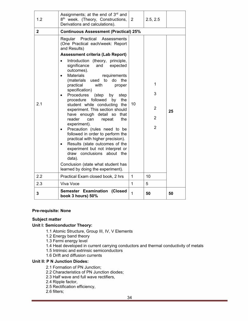
Assessment approach:
Sl. No. Mode of Assessment Nos. Marks Allocated
Marks (%)
1 Continuous Assessment (Theory) 25%
1.1
Term Tests: Closed book, one hour duration in 5th and 10th week. (Theory, Constructions, Derivations and calculations).
Two units will be covered for term I and three for term II. (Theory, Constructions, Derivations and calculations).
2 20 25
34
1.2 Assignments; at the end of 3rd and 8th week. (Theory, Constructions, Derivations and calculations).
2 2.5, 2.5
2 Continuous Assessment (Practical) 25%
2.1
Regular Practical Assessments (One Practical each/week: Report and Results)
Assessment criteria (Lab Report)
Introduction (theory, principle, significance and expected outcomes).
Materials requirements (materials used to do the practical with proper specification)
Procedures (step by step procedure followed by the student while conducting the experiment. This section should have enough detail so that reader can repeat the experiment).
Precaution (rules need to be followed in order to perform the practical with higher precision).
Results (state outcomes of the experiment but not interpret or draw conclusions about the data).
Conclusion (state what student has learned by doing the experiment).
10
1
3
2
2
2
25
2.2 Practical Exam closed book, 2 hrs 1 10
2.3 Viva Voce 1 5
3 Semester Examination (Closed book 3 hours) 50%
1 50 50
Pre-requisite: None
Subject matter
Unit I: Semiconductor Theory:
1.1 Atomic Structure, Group III, IV, V Elements 1.2 Energy band theory 1.3 Fermi energy level 1.4 Heat developed in current carrying conductors and thermal conductivity of metals 1.5 Intrinsic and extrinsic semiconductors 1.6 Drift and diffusion currents
Unit II: P N Junction Diodes:
2.1 Formation of PN Junction; 2.2 Characteristics of PN Junction diodes; 2.3 Half wave and full wave rectifiers, 2.4 Ripple factor, 2.5 Rectification efficiency, 2.6 filters;
35
2.7 Interpretation of Data Sheet for Diodes; 2.8 Zener diodes, its characteristics & use as a simple voltage regulator; 2.9 Construction, working principles of Clippers, 2.10 Construction, working principles of Clampers, 2.11 Peak detectors; 2.12 General idea about LED, 2.13 Photodiodes, 2.14 Schottky diodes
Unit III: Transistors:
3.1 Bipolar transistors, symbols and basic construction 3.2 Amplification action 3.3 Transistor currents; CE, CB & CC configurations & corresponding characteristics 3.4 BJT as a switch 3.5 Analysis of biasing circuits 3.6 Stability factor 3.7 Thermal stabilization and run away 3.8 h-parameter and remodel equivalent circuits 3.9 Small signal analysis of transistor amplifiers 3.10 Amplification, derivation of expressions for voltage gain, current gain, input and output
impedance of CC, CB and CE configuration, with more focus on CE configuration; 3.11 Design of a single stage CE amplifiers using data sheet of appropriate components;
General idea about JFET, FET, CMOS, MOSFET with characteristics
Unit IV: Silicon wafer fabrication,
4.1 Different techniques involved in Silicon wafer fabrication.
Unit V: Power amplifiers:
5.1 Classification of Power amplifier 5.2 Distortion 5.3 Description of RC coupled and transformer coupled and direct coupled amplifiers 5.4 Class A and Class B type amplifiers both transformers coupled and transformer less
List of Practical’s:
1. To plot characteristics of pn junction diode
2. Study of half-wave rectifier circuit using pn junction diodes
3. Study of full-wave rectifiers without and with Filters
4. Study of basic Clipper Circuits
5. Study of basic Clamper Circuits
6. Study Characteristics Zener diode and its application as voltage regulator
7. Characteristics of bipolar junction Transistor
8. Construction of Single stage amplifier and its analysis
9. Analysis of Cross Over Distortion in Power amplifiers
10. Efficiency of Power amplifiers – Class A or Class B
Reading List
Essential Reading:
1. Millman, J. & Halkias, C. C. (2003), Integrated Electronics, Analog and Digital circuits and Systems, (4 ed.), Tata McGraw Hill, New Delhi.
2. Malvino (1999), Electronics Principles, (6 ed.), Tata McGraw Hill, New Delhi.
36
3. Boyelstad, R. L. & Nashelsky, L. (2004), Electronics Devices and Circuit Theory, (6 ed.) , PHI, New Delhi.
4. Gayakwad, R. A. (2002), Op-Amp and Linear Integrated Circuits, (4 ed.), Pearson Education Asia, New Delhi.
Additional Reading
1. Rashid, M. H (1995), Microelectronic Circuits: Analysis and Design, (1 ed.), PWS Publishing Company, New Delhi.
Date: February 4, 2017
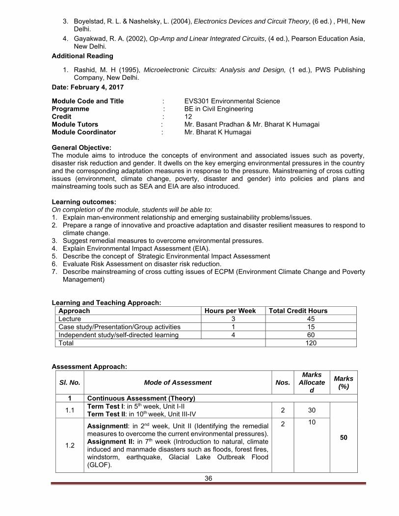
Module Code and Title : EVS301 Environmental Science Programme : BE in Civil Engineering Credit : 12 Module Tutors : Mr. Basant Pradhan & Mr. Bharat K Humagai Module Coordinator : Mr. Bharat K Humagai General Objective: The module aims to introduce the concepts of environment and associated issues such as poverty, disaster risk reduction and gender. It dwells on the key emerging environmental pressures in the country and the corresponding adaptation measures in response to the pressure. Mainstreaming of cross cutting issues (environment, climate change, poverty, disaster and gender) into policies and plans and mainstreaming tools such as SEA and EIA are also introduced. Learning outcomes: On completion of the module, students will be able to: 1. Explain man-environment relationship and emerging sustainability problems/issues. 2. Prepare a range of innovative and proactive adaptation and disaster resilient measures to respond to
climate change. 3. Suggest remedial measures to overcome environmental pressures. 4. Explain Environmental Impact Assessment (EIA). 5. Describe the concept of Strategic Environmental Impact Assessment 6. Evaluate Risk Assessment on disaster risk reduction. 7. Describe mainstreaming of cross cutting issues of ECPM (Environment Climate Change and Poverty
Management) Learning and Teaching Approach:
Approach Hours per Week Total Credit Hours Lecture 3 45 Case study/Presentation/Group activities 1 15 Independent study/self-directed learning 4 60 Total 120
Assessment Approach:
Sl. No. Mode of Assessment Nos. Marks
Allocated
Marks (%)
1 Continuous Assessment (Theory)
1.1 Term Test I: in 5th week, Unit I-II Term Test II: in 10th week, Unit III-IV
2 30
50 1.2
AssignmentI: in 2nd week, Unit II (Identifying the remedial measures to overcome the current environmental pressures).Assignment II: in 7th week (Introduction to natural, climate induced and manmade disasters such as floods, forest fires, windstorm, earthquake, Glacial Lake Outbreak Flood (GLOF).
2 10
37
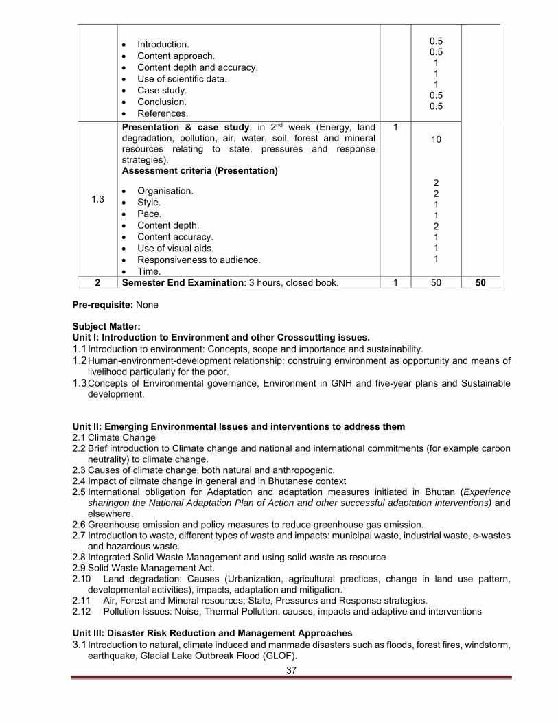
Pre-requisite: None Subject Matter: Unit I: Introduction to Environment and other Crosscutting issues. 1.1 Introduction to environment: Concepts, scope and importance and sustainability. 1.2 Human-environment-development relationship: construing environment as opportunity and means of
livelihood particularly for the poor. 1.3 Concepts of Environmental governance, Environment in GNH and five-year plans and Sustainable
development. Unit II: Emerging Environmental Issues and interventions to address them 2.1 Climate Change 2.2 Brief introduction to Climate change and national and international commitments (for example carbon
neutrality) to climate change. 2.3 Causes of climate change, both natural and anthropogenic. 2.4 Impact of climate change in general and in Bhutanese context 2.5 International obligation for Adaptation and adaptation measures initiated in Bhutan (Experience
sharingon the National Adaptation Plan of Action and other successful adaptation interventions) and elsewhere.
2.6 Greenhouse emission and policy measures to reduce greenhouse gas emission. 2.7 Introduction to waste, different types of waste and impacts: municipal waste, industrial waste, e-wastes
and hazardous waste. 2.8 Integrated Solid Waste Management and using solid waste as resource 2.9 Solid Waste Management Act. 2.10 Land degradation: Causes (Urbanization, agricultural practices, change in land use pattern,
developmental activities), impacts, adaptation and mitigation. 2.11 Air, Forest and Mineral resources: State, Pressures and Response strategies. 2.12 Pollution Issues: Noise, Thermal Pollution: causes, impacts and adaptive and interventions Unit III: Disaster Risk Reduction and Management Approaches 3.1 Introduction to natural, climate induced and manmade disasters such as floods, forest fires, windstorm,
earthquake, Glacial Lake Outbreak Flood (GLOF).
Introduction. Content approach. Content depth and accuracy. Use of scientific data. Case study. Conclusion. References.
0.5 0.5 1 1 1
0.5 0.5
1.3
Presentation & case study: in 2nd week (Energy, land degradation, pollution, air, water, soil, forest and mineral resources relating to state, pressures and response strategies). Assessment criteria (Presentation)
Organisation. Style. Pace. Content depth. Content accuracy. Use of visual aids. Responsiveness to audience. Time.
1 10
2 2 1 1 2 1 1 1
2 Semester End Examination: 3 hours, closed book. 1 50 50
38
3.2 Causes and impacts of disasters. 3.3 Disaster Risk Analysis/ Risk Assessment and Disaster Risk Reduction 3.4 Innovative and proactive measures, including non-structural mitigation measures (falling hazards)
initiated in Bhutan and beyond in managing and reducing the risk of disaster. Unit IV: Environmental Impact Assessment (EIA) 4.1 Principles and theoretical background of Environmental Impact Assessment (EIA), including social
impact assessment (SIA). 4.2 Introduction to SEA, Difference between SEA and EIA, Rationale and importance/benefit of SEA,
Challenges of conducting SEA, limitation and emerging criticism on SEA. Unit V: Mainstreaming of cross cutting issue (ECP, DRR and Gender) into development policies, plan and programs 5.1 Concepts of mainstreaming, approaches and tools for mainstreaming, challenges. 5.2 Mainstreaming of ECPM into Development policies, plans and programmes in Bhutan. Reading Lists: Essential Reading 1. Canter, L.W. (1996). Environmental Impact Assessment. Singapore: McGraw-Hill, Inc. 2. Davis, H.L., & Masten, S.J. (2004). Principles of Environmental Engineering & Sciences. New York,
NY: McGraw Hill 3. Masters, G.M. (1991). Introduction to Environmental Engineering and Science, New Delhi: Prentice-
Hall India Pvt. Ltd. 4. Nebel, B. J., (1987).Environmental Science, Prentice-Hall Inc. 5. Therivel, R. (2004). Strategic Environmental Assessment in Action. London: Earthsca Additional Reading 1. Clayton, B.D., & Bass, S. (2009). The challenges of environmental mainstreaming: Experience
ofintegrating environment into development institutions and decisions. London: EnvironmentalGovernance No.3. International Institute for Environment and Development.
2. Clayton, B.D., & Sadler, B. (2005). Strategic Environmental Assessment: A sourcebook andreference guide to international experience. London: Earthscan.
3. Wright, R.T., & Nebel, B.J. (2002). Environmental Science: Towards a Sustainable Future. 6. Cunningham,W.P., & Cunningham, M. A. (2007). Principles of Environmental Science: Inquiry &
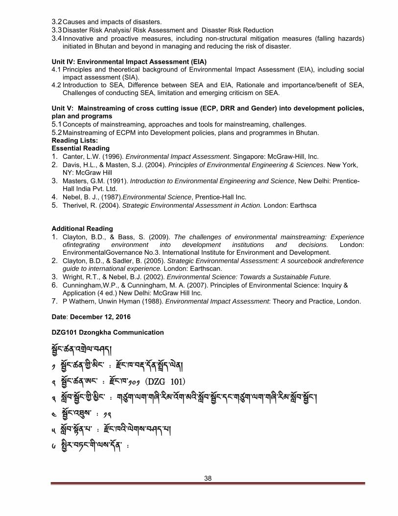
Application (4 ed.) New Delhi: McGraw Hill Inc. 7. P Wathern, Unwin Hyman (1988). Environmental Impact Assessment: Theory and Practice, London. Date: December 12, 2016 DZG101 Dzongkha Communication
སྦྱོང་ཚན་འགྲེལ་བཤད། ༡ སྦྱོང་ཚན་གྱི་མིང་ : རྫངོ་ཁ་བརྡ་དནོ་སྤྲོད་ལེན། ༢ སྦྱོང་ཚན་ཨང་ : རྫངོ་ཁ་༡༠༡ (DZG 101) ༣ སོླབ་སོྦྱང་གྱི་མྱིང་ : གཙུག་ལག་གཞི་རིམ་འོག་མའི༌སོླབ་སྦྱངོ་དང་གཙུག་ལག་གཞི་རིམ་སོླབ་སོྦྱང་། ༤ སྦྱོང་འཐུས་ : ༡༢ ༥ སོླབ་སོྟན་པ་ : རྫངོ་ཁའི་ལེགས་བཤད་པ། ༦ སྤྱིར་བཏང་གི་ལས་དོན་ :
39
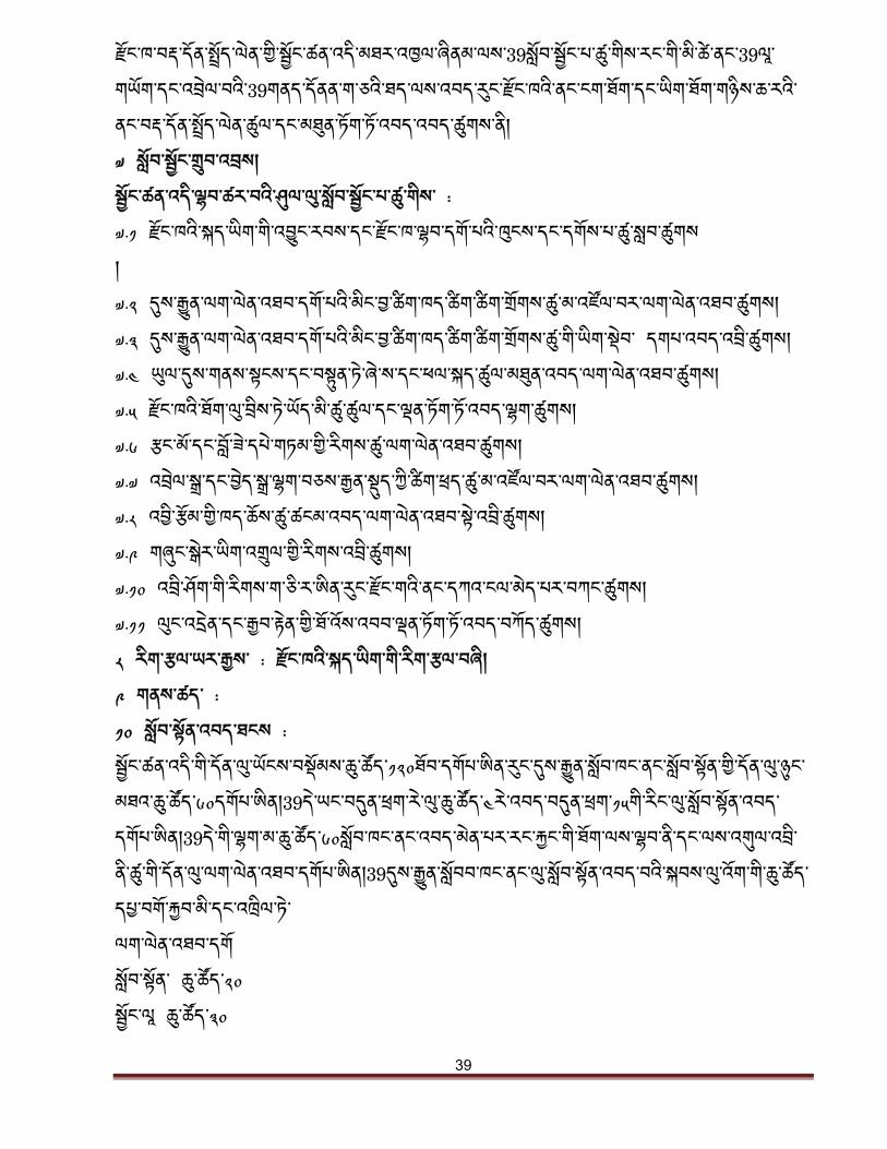
རྫོང་ཁ་བརྡ་དོན་སོྤྲད་ལེན་གྱི་སོྦྱང་ཚན་འདི་མཐར་འཁྱལ་ཞིནམ་ལས་39སོླབ་སོྦྱང་པ་ཚུ་གིས་རང་གི་མི་ཚེ་ནང་39ལཱ་གཡོག་དང་འབྲེལ་བའི་39གནད་དོནན་ག་ཅའི་ཐད་ལས་འབད་རུང་རོྫང་ཁའི་ནང་ངག་ཐོག་དང་ཡིག་ཐོག་གཉིས་ཆ་རའི་ནང་བརྡ་དོན་སོྤྲད་ལེན་ཚུལ་དང་མཐུན་ཏོག་ཏོ་འབད་འབད་ཚུགས་ནི། ༧ སློབ་སྦྱངོ་གྲུབ་འབྲས། སྦྱོང་ཚན་འདི་ལྷབ་ཚར་བའི་ཤུལ་ལུ་སོླབ་སྦྱོང་པ་ཚུ་གིས་ : ༧.༡ རོྫང་ཁའི་སྐད་ཡིག་གི་འབྱུང་རབས་དང་རོྫང་ཁ་ལྷབ་དགོ་པའི་ཁུངས་དང་དགོས་པ་ཚུ་སླབ་ཚུགས ། ༧.༢ དུས་རྒྱུན་ལག་ལེན་འཐབ་དགོ་པའི་མིང་བྱ་ཚིག་ཁད་ཚིག་ཚིག་གྲོགས་ཚུ་མ་འཛོལ་བར་ལག་ལེན་འཐབ་ཚུགས། ༧.༣ དུས་རྒྱུན་ལག་ལེན་འཐབ་དགོ་པའི་མིང་བྱ་ཚིག་ཁད་ཚིག་ཚིག་གྲོགས་ཚུ་གི་ཡིག་སྡེབ་ དགཔ་འབད་འབྲི་ཚུགས། ༧.༤ ཡུལ་དུས་གནས་སྟངས་དང་བསྟུན་ཏེ་ཞེ་ས་དང་ཕལ་སྐད་ཚུལ་མཐུན་འབད་ལག་ལེན་འཐབ་ཚུགས། ༧.༥ རྫོང་ཁའི་ཐོག་ལུ་བྲིས་ཏེ་ཡོད་མི་ཚུ་ཚུལ་དང་ལྡན་ཏོག་ཏ་ོའབད་ལྷག་ཚུགས། ༧.༦ རྩང་མོ་དང་བླ་ོཟེ་དཔེ་གཏམ་གྱི་རིགས་ཚུ་ལག་ལེན་འཐབ་ཚུགས། ༧.༧ འབྲེལ་སྒྲ་དང་བྱེད་སྒྲ་ལྷག་བཅས་རྒྱན་སྡུད་ཀྱི་ཚིག་ཕྲད་ཚུ་མ་འཛོལ་བར་ལག་ལེན་འཐབ་ཚུགས། ༧.༨ འབྱི་རོྩམ་གྱི་ཁད་ཆོས་ཚུ་ཚངམ་འབད་ལག་ལེན་འཐབ་སྟེ་འབྲི་ཚུགས། ༧.༩ གཞུང་སྒེར་ཡིག་འགྲུལ་གྱི་རིགས་འབྲི་ཚུགས། ༧.༡༠ འབྲི་ཤོག་གི་རིགས་ག་ཅི་ར་ཨིན་རུང་རྫོང་གའི་ནང་དཀའ་ངལ་མེད་པར་བཀང་ཚུགས། ༧.༡༡ ལུང་འདྲེན་དང་རྒྱབ་རྟེན་གྱི་ཐོ་འོས་འབབ་ལྡན་ཏོག་ཏོ་འབད་བཀོད་ཚུགས། ༨ རིག་རྩལ་ཡར་རྒྱས་ : རྫངོ་ཁའི་སྐད་ཡིག་གི་རིག་རྩལ་བཞི། ༩ གནས་ཚད་ : ༡༠ སློབ་སྟོན་འབད་ཐངས : སོྦྱང་ཚན་འདི་གི་དོན་ལུ་ཡོངས་བསོྡམས་ཆུ་ཚོད་༡༢༠ཐོབ་དགོཔ་ཨིན་རུང་དུས་རྒྱུན་སོླབ་ཁང་ནང་སོླབ་སོྟན་གྱི་དོན་ལུ་ཉུང་མཐའ་ཆུ་ཚོད་༦༠དགོཔ་ཨིན།39དེ་ཡང་བདུན་ཕྲག་རེ་ལུ་ཆུ་ཚོད་༤རེ་འབད་བདུན་ཕྲག་༡༥གི་རིང་ལུ་སོླབ་སོྟན་འབད་དགོཔ་ཨིན།39དེ་གི་ལྷག་མ་ཆུ་ཚོད་༦༠སོླབ་ཁང་ནང་འབད་མེན་པར་རང་རྐྱང་གི་ཐོག་ལས་ལྷབ་ནི་དང་ལས་འགུལ་འབྲི་ནི་ཚུ་གི་དོན་ལུ་ལག་ལེན་འཐབ་དགོཔ་ཨིན།39དུས་རྒྱུན་སོླབབ་ཁང་ནང་ལུ་སོླབ་སོྟན་འབད་བའི་སྐབས་ལུ་འོག་གི་ཆུ་ཚོད་དཔྱ་བགོ་རྐྱབ་མི་དང་འཁྲིལ་ཏེ་ ལག་ལེན་འཐབ་དགོ སོླབ་སོྟན་ ཆུ་ཚོད་༢༠ སོྦྱང་ལཱ ཆུ་ཚོད་༣༠
40
སྤྱན་ཞུ་ ཆུ་ཚདོ་༡༠ ༡༡ དབྱེ་ཞིབ་ : སོྦྱང་ཚན་འདི༌གི༌དོན་ལུ་སྦྱང་རྒྱུགས་དབྱེ༌ཞིབ་དང་དུས་རྒྱུན་དབྱེ་ཞིབ་གཉིས་ཆ་ར་ལག་ལེན་འཐབ་སྟེ་དབྱེ་ཞིབ་འབད་དགོཔ་ཨིན། ཀ དུས་རྒྱུན་དབྱེ་ཞིབ།སྐུགས་༥༠%
ལས་འགུལ་ ༢༠% སོླབ་ཁང་སྤྱན་ཞུ་ ༡༥% སོླབ་ཁང་གི་སོྦྱང་ལཱ་ ༡༥%
ཁ་ སྦྱང་རྒྱུགས་དབྱེ་ཞིབ། ༥༠% ཆོས་རྒྱུགས། ༥༠% ཡོངས་བསོྡམས་སྐུགས་ ༡༠༠
༡༢ སྔོན་ཚང་ཤེས་ཡོན་ : ༡༣ ནང་དོན་ དོན་ཚན་ཀ་པ། སྐད་ཡིག་གྱི་ངོ་སོྦྱད། (ཆུ་ཚོད་༣) ༡ རྫོང་ཁའི་སྐད་ཡིག་གི་འབྱུང་རབས། ༢ རྫོང་ཁ་ལྷབ་དགོ་པའི་དགོས་པ། དོན་ཚན་ཁ་པ། མིང་ཚིག་བརྗོད་པའི་རྣམ་གཞག (ཆུ་ཚདོ་༢༥) ༡ མིང་། ༢ བྱ་ཚིག་ ༣ ཁྱད་ཚིག་ ༤ ཚིག་གྲོགས། ༥ རོྫང་ཁ་ངག་གཤིས་འགྲོ་ལུགས། ༦ སྙན་རྩོམ། དཔེ་གཏམ། བོླ་ཟེ། རྩང་མོ། ༧ རྫོང་ཁ་ཁ་ཉག་རྐྱང་གི་མིང་ཚིག་ལག་ལེན་འཐབ་ཐངས། ༨ མིང་ཚིག་དང་བྱ་ཚིག་ཁྱད་ཚིག་ཚུ་འོས་འབབ་ལྡནམ་འབད་ལག་ལེན་འཐབ་ཐངས།
དོན་ཚན་ག་པ། རོྫང་ཁའི་ངག་གཤིས་དང་འཁྲིལ་ཏེ་ལྷག་ཐངས། (ཆུ་ཚོད་༤) ༡ ཚིག་མཚམས་བཅད་དེ་ལྷག་ཐངས། ༢ རྗེས་འཇུག་གི་སྒྲ་ཧྲིལ་བུ་བཏོན་དགོཔ་དང་མ་དགོ་པའི་རིགས་ཚུ་ཁྱད་པར་ཕྱེ་སྟེ་ལྷག་ཐངས།
41
༣ རྗེས་འཇུག་མེད་རུང་ཡོདཔ་བཟུམ་ལྷག་ཐངས། དོན་ཚན་ང་པ། ཡི་གུའི་སོྦྱར་བ། (ཆུ་ཚོད་༨) ༡ འབྲེལ་སྒྲ། ༢ བྱེད་སྒྲ། ༣ ལྷག་བཅས། ༤ རྒྱན་སྡུད།
དོན་ཚན་ཅ་པ། ཡིག་འགྲུལ། (ཆུ་ཚོད་༢༠)
༡ ཡིག་ཅུང་འབྲི་ཐངས། ༢ མགྲོན་ཞུ་འབྲི་ཐངས། ༣ གཏང་ཡིག་འབྲི་ཐངས། ༤ ཞུ་ཡིག་དང་ཞུ་ཚིག་/བཤེར་ཡིག་འབྲི་ཐངས། ༥ གན་ཡིག་འབྲི་ཐངས། ༦ སྙན་ཞུ་འབྲི་ཐངས། ༧ གྲོས་ཆོད་འབྲི་ཐངས། ༨ ཁྱབ་བསྒྲགས་ཀྱི་རིགས་འབྲི་ཐངས། ༩ འབྲི་ཤོག་གི་རིགས་བཀང་ཐངས། ༡༠ འབྲི་རོྩམ་འབྲི་ཐངས། ༡༡ ཚག་ཤད་ལག་ལེན་འཐབ་ཐངས། ༡༢ ལུང་འདྲེན་དང་རྒྱབ་ཏེན་གྱི་དཔེ་ཐོ་བཀོད་ཐངས།
དོན་ཚན་ཆ་པ། སྐད་སྒྱུར།
༡༤ ལྷག་དགོ་པའི་དཔེ་ཐོ། ཀ སོྦྱང་ཚན་འདི་སྦྱང་བ་ལེགས་ཤོམ་འབད་ཐོབ་ནིའི་དོན་ལུ་འོག་ལུ་བཀོད་དེ་ཡོད་མའི་དཔེ་དེབ་ཚུ་ངེས་པར་དུ་ལྷག་དགོ ཀུན་བཟང་རོྡ་རྗེ། (༢༠༡༡) བོླ་ཟེ་ལྷའི་པི་ཝང་། ཐིམ་ཕུ། རྫོང་ཁ་གོང་འཕེལ་ལྷན་ཚོགས། ཀུན་བཟང་རོྡ་རྗེ། (༢༠༡༡) རྩང་མོའི་ཀྱི་དེབ་བོླ་རིག་མེ་ཏོག ཐིམ་ཕུ། རོྫང་ཁ་གོང་འཕེལ་ལྷན་ཚོགས། ཀུན་བཟང་འཕྲིན་ལས། (༢༠༠༡) ཡིག་བསྐུར་རྣམ་གཞག་གི་དེབ། ཐིམ་ཕུ། ཀེ་ཨེམ་ཀྲི།
42
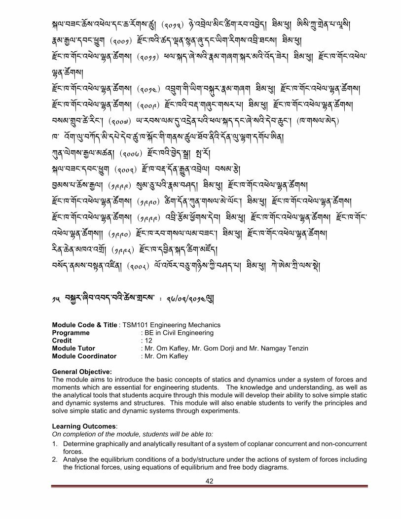
སྐལ་བཟང་ཆོས་འཕེལ་དང་ཆ་རོགས་ཚུ། (༢༠༡༣) ཉེ་འབྲེལ་མིང་ཚིག་རབ་འབྱེད། ཐིམ་ཕུ། ཨིསི་ཀྲུ་གྲེན་པ་ལཱསི། རྣམ་རྒྱལ་དབང་ཕྱུག (༢༠༠༡) རྫོང་ཁའི་ཚད་ལྡན་སྙན་ཞུ་དང་ཡིག་རིགས་འབྲི་ཐངས། ཐིམ་ཕུ། རྫོང་ཁ་གོང་འཕེལ་ལྷན་ཚོགས། (༢༠༡༡) ཕལ་སྐད་ཞེ་སའི་རྣམ་གཞག་སྐར་མའི་འོད་ཟེར། ཐིམ་ཕུ། རྫོང་ཁ་གོང་འཕེལ་ལྷན་ཚོགས། རྫོང་ཁ་གོང་འཕེལ་ལྷན་ཚོགས། (༢༠༡༤) འབྲུག་གི་ཡིག་བསྐུར་རྣམ་གཞག ཐིམ་ཕུ། རྫོང་ཁ་གོང་འཕེལ་ལྷན་ཚོགས། རྫོང་ཁ་གོང་འཕེལ་ལྷན་ཚོགས། (༢༠༠༩) རྫོང་ཁའི་བརྡ་གཞུང་གསར་པ། ཐིམ་ཕུ། རོྫང་ཁ་གོང་འཕེལ་ལྷན་ཚོགས། བསམ་གྲུབ་ཚེ་རིང་། (༢༠༠༧) ཡ་རབས་ལམ་དུ་འདྲེན་པའི་ཕལ་སྐད་དང་ཞེ་སའི་དེབ་ཆུང་། (ཁ་གསལ་མེད) ཁ་ འོག་ལུ་བཀོད་མི་དཔེ་དེབ་ཚུ་ཁ་སྐོང་གི་གནས་ཚུལ་ཐོབ་ནིའི་དོན་ལུ་ལྷག་དགོཔ་ཨིན། ཀུན་ལེགས་རྒྱལ་མཚན། (༢༠༠༦) རོྫང་ཁའི་བྱེད་སྒྲ། སྤ་རོ། སྐལ་བཟང་དབང་ཕྱུག (༢༠༠༢) རྫོ་ཁ་བརྡ་དོན་རྒྱུན་འབྲེལ། བསམ་རྩེ། བྱམས་པ་ཆོས་རྒྱལ། (༡༩༩༩) སུམ་ཅུ་པའི་རྣམ་བཤད། ཐིམ་ཕུ། རྫོང་ཁ་གོང་འཕེལ་ལྷན་ཚོགས། རྫོང་ཁ་གོང་འཕེལ་ལྷན་ཚོགས། (༡༩༩༠) ཚིག་དོན་ཀུན་གསལ་མེ་ལོང༌། ཐིམ་ཕུ། རོྫང་ཁ་གོང་འཕེལ་ལྷན་ཚོགས། རྫོང་ཁ་གོང་འཕེལ་ལྷན་ཚོགས། (༡༩༩༩) འབྲི་རོྩམ་ཕོྱགས་དེབ། ཐིམ་ཕུ། རྫོང་ཁ་གོང་འཕེལ་ལྷན་ཚོགས། རྫོང་ཁ་གོང་འཕེལ་ལྷན་ཚོགས།། (༡༩༩༠) རོྫང་ཁ་རབ་གསལ་ལམ་བཟང༌། ཐིམ་ཕུ། རྫོང་ཁ་གོང་འཕེལ་ལྷན་ཚོགས། རིན་ཆེན་མཁའ་འགྲོ། (༡༩༩༨) རོྫང་ཁ་དབྱིན་སྐད་ཚིག་མཛོད། བསོད་ནམས་བསྟན་འཛིན། (༢༠༠༨) ལོ་འཁོར་བཅུ་གཉིས་ཀྱི་བཤད་པ། ཐིམ་ཕུ། ཀེ་ཨེམ་ཀྲི་ལས་སྡེ། ༡༥ བསྐྱར་ཞིབ་འབད་བའི་ཚེས་གྲངས་ : ༢༦/༠༢/༢༠༡༤ལུ། Module Code & Title : TSM101 Engineering Mechanics Programme : BE in Civil Engineering Credit : 12 Module Tutor : Mr. Om Kafley, Mr. Gom Dorji and Mr. Namgay Tenzin Module Coordinator : Mr. Om Kafley General Objective: The module aims to introduce the basic concepts of statics and dynamics under a system of forces and moments which are essential for engineering students. The knowledge and understanding, as well as the analytical tools that students acquire through this module will develop their ability to solve simple static and dynamic systems and structures. This module will also enable students to verify the principles and solve simple static and dynamic systems through experiments. Learning Outcomes: On completion of the module, students will be able to:
1. Determine graphically and analytically resultant of a system of coplanar concurrent and non-concurrent forces.
2. Analyse the equilibrium conditions of a body/structure under the actions of system of forces including the frictional forces, using equations of equilibrium and free body diagrams.
43
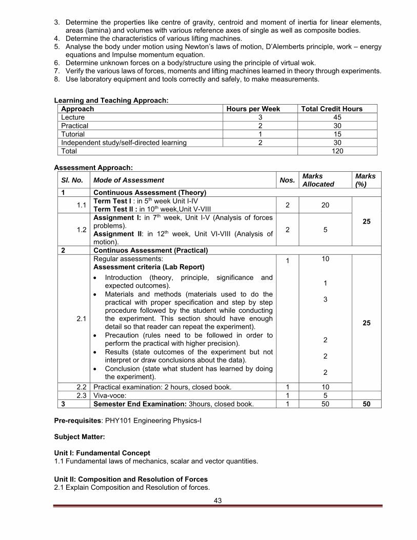
3. Determine the properties like centre of gravity, centroid and moment of inertia for linear elements, areas (lamina) and volumes with various reference axes of single as well as composite bodies.
4. Determine the characteristics of various lifting machines. 5. Analyse the body under motion using Newton’s laws of motion, D’Alemberts principle, work – energy
equations and Impulse momentum equation. 6. Determine unknown forces on a body/structure using the principle of virtual wok. 7. Verify the various laws of forces, moments and lifting machines learned in theory through experiments. 8. Use laboratory equipment and tools correctly and safely, to make measurements.
Learning and Teaching Approach:
Approach Hours per Week Total Credit Hours Lecture 3 45 Practical 2 30 Tutorial 1 15 Independent study/self-directed learning 2 30 Total 120
Assessment Approach:
Sl. No. Mode of Assessment Nos. Marks Allocated
Marks (%)
1 Continuous Assessment (Theory)
1.1 Term Test I : in 5th week Unit I-IV Term Test II : in 10th week,Unit V-VIII
2 20
25 1.2
Assignment I: in 7th week, Unit I-V (Analysis of forces problems). Assignment II: in 12th week, Unit VI-VIII (Analysis of motion).
2 5
2 Continuos Assessment (Practical)
2.1
Regular assessments: Assessment criteria (Lab Report)
Introduction (theory, principle, significance and expected outcomes).
Materials and methods (materials used to do the practical with proper specification and step by step procedure followed by the student while conducting the experiment. This section should have enough detail so that reader can repeat the experiment).
Precaution (rules need to be followed in order to perform the practical with higher precision).
Results (state outcomes of the experiment but not interpret or draw conclusions about the data).
Conclusion (state what student has learned by doing the experiment).
1 10
1
3
2
2
2
25
2.2 Practical examination: 2 hours, closed book. 1 10 2.3 Viva-voce: 1 5
3 Semester End Examination: 3hours, closed book. 1 50 50 Pre-requisites: PHY101 Engineering Physics-I Subject Matter: Unit I: Fundamental Concept 1.1 Fundamental laws of mechanics, scalar and vector quantities.
Unit II: Composition and Resolution of Forces 2.1 Explain Composition and Resolution of forces.
44
2.2 Find resultant using Analytical and graphical method. 2.3 Composition of forces by Resolution. Unit III: Moments and Couples 3.1 Moment of force and Varignon’s theorem. 3.2 Couple and resultant of a force system. 3.3 Type of levers. Unit IV: Equilibrium 4.1 Equilibrium of a body, Equilibrant. 4.2 Type of forces on a body, Free Body Diagrams. 4.3 Lami’s theorem. 4.4 Equilibrium of connected bodies, Equilibrium conditions. 4.5 Reaction, loading and support of beams. Unit V: Friction 5.1 Frictional force and laws of frictions. 5.2 Angle of friction, angle of cone, angle of repose. 5.3 Wedges, Rope friction, Non-concurrent force problems. Unit VI: Centre of Gravity and Moment of Inertia 6.1. Centre of gravity, Centre of gravity of a flat plate and solid, centroid, axis of symmetry. 6.2. Centre of gravity from first principal and centre of composite section. 6.3. Moment of inertia, Polar moment of inertia and Radius of gyration. 6.4. Theorems of moment of inertia, moment of inertia from first principle, moment of inertia of standard
section and composite section including the mass moment of inertia. Unit VII: Principle of Lifting Machines 7.1. Law of machine, Mechanical advantage. 7.2. Differential wheel and axle, winch crab (single and double), worm and worm wheel, inclined plane. Unit VIII: Linear Motion, Motion of Rotation and Translation 8.1. General principle of dynamics, type of motion. 8.2. Newton’s law of motion I, II, and III, D’ Alembert's principle. 8.3. Work, power and energy, Work-energy equation, Work done by a spring. 8.4. Impulse momentum equation, conservation of momentum, pile and hammer. 8.5. Kinematics of motion of rotation, Angular momentum and its application. 8.6. Acceleration during circular motion, motion on level road, designed speed, skidding and
overturning. 8.7. Angular motion, kinetic energy of rotating bodies, relation between angular motion and linear
motion. 8.8. Motion of connected bodies. 8.9. Combined motion of rotation and translation.
Unit IX: Virtual Work 9.1. Principle of Virtual Work. 9.2. Application of the principle of virtual work to determine unknown forces. List of Practicals:
1. Verification of Triangle law of forces. 2. Verification of Polygon law of forces. 3. Verification of Parallelogram law of forces. 4. Determine the Co-efficient of Friction for rolling and sliding friction for different surfaces. 5. Determination of Law of Machine for Worm and Worm Wheel, Single Purchase Winch Crab, Differential
Wheel and Axle. 6. Verify Principle of Moment.
Reading Lists:
45
Essential Reading
1. Meriam, J. L. & Kraige, L. G. (2013). Engineering Mechanics - Statics (7 ed.). New Delhi: Wiley India. 2. Bhavikatti, S. S. & Rajashekarappa, K. G. (2004). Engineering Mechanics. New Delhi: New Age
International Publishers. 3. Timoshenko, S. & Young, D. H. (2006). Engineering Mechanics. New Jersey: McGraw Hill
Publications. 4. Hibbeler, R. C. (2013). Engineering Mechanics-Statics (13 ed.). New Jersey: Pearson Prentice Hall,
Pearson Education.
Additional Reading
1. Kumar, K. L. (1998). Engineering Mechanics. New Delhi: McGraw Hill. 2. Malhotra, D. R. & Gupta, H. C. (1998). Applied Mechanics & Strength of Materials. New Delhi:
Satyaprakashan Publishers, 3. Shigley. (2000). Applied Mechanics of Materials. New Delhi: McGraw Hill Publications, International
Student Edition. 4. Khurmi, R. S. (2002). Text Book of Engineering Mechanics. New Delhi: S.Chand & Co. 5. Sinha, N. C. & Sen Gupta, S. K. (1987). Elements of Structural Mechanics. New Delhi: S.Chand & Co. 6. Junarkar, S. B. (1991). Elements of Applied Mechanics. New Delhi: Charotar Publications, Anand. 7. Ramamrutham, S. (2001). A Text Book of Applied Mechanics. New Delhi: Dhanpat Rai Publications. 8. Malhotra, M. M. etc. Al. (1994). A Text Book in Applied Mechanics. New Delhi: New Age International
Publishers. 9. Shames, Irving. H. (1996). Engineering Mechanics–Statics & Dynamics. New Delhi: Prentice Hall India.
Date: March 5, 2016 Module Code & Title : ACS101 Academic Skills Programme : RUB-wide module Credit : 12 Module Tutor : Mrs. Chencho Dema General Objective: The Academic Skills module is designed to support students in their learning and provide generic skills that are required for university study. The focus will be on developing the skills of academic writing, oral presentation, and research skills, which will be delivered through classroom instruction, as well as through course work.
Learning Outcomes: On completion of the module, students will be able to:
1. Communicate effectively in both spoken and written academic forms. 2. Select relevant information from a range of textual formats and synthesize through note taking,
summarizing and paraphrasing and reformulate it in written and spoken form. 3. Read texts at a variety of levels by applying skimming and scanning techniques, and reading for
detailed understanding. 4. Evaluate the credibility of sources (i.e. by author, publisher or website). 5. Organise writing according to purpose of writing and text types through planning, organizing ideas,
structuring, synthesizing, editing and proofreading. 6. Develop own arguments and integrate these appropriately with source material in written and spoken
form in line with the concepts of academic integrity. 7. Cite sources and create a reference list using APA style. 8. Deliver a formal academic oral presentation. 9. Critically reflect on their own learning by organizing their learning and monitoring its progress by
maintaining a portfolio. 10. Appreciate and develop personal skills such as cooperation, negotiation, group work, and leadership. 11. Develop an independent approach to studying.
46
Learning and Teaching Approach: Tutors will employ an interactive, student-centred approach, integrating language and critical thinking skills using the following strategies over the 60 hours of contact time. 1. Demonstrations/Modelling (3 hours) 2. Practical exercises and activities/Task-based learning (18 hours) 3. Individual, pair and group work (e.g. Discussions, problem-solving activities, collaborative and
individual tasks, peer feedback, debates, role-plays, etc.) (18 hours) 4. Process learning, with diagnosis, feedback and remediation (e.g., with portfolio tasks) (15 hours) 5. Presentations (6 hours)
Assessment Approach: Since this module is entirely assessed through coursework, a student must complete all 4 components of the assessment outlined below (portfolio; 2 class tests; presentation; essay) and get an aggregate mark of 50% in order to pass.
Sl. No. Mode of Assessment Nos. Marks Allocated
Marks (%)
1 Continuous Assessment (Theory)
1.1 A Portfolio of work done in class and as homework 1 25
100 1.2 Class Tests 2 30
1.3 An Oral Presentation 1 15
1.4 A Researched Assignment (essay) 1 30 Pre-requisite: None
Subject Matter:
Unit1: Academic Standard Ethics (5 hours) 1.1. Purpose of academic activity 1.2. Features of academic writing 1.3. Academic argument and academic integrity
Unit 2: Note-taking (6 hours) 2.1. Basics of note-taking 2.2. Types of notes, strategies and activities 2.3. Listening and note-taking
Unit3: Academic Reading (13hours) 3.1 Identify text features &organization 3.2 Reading Techniques(skimming/scanning, SQ3R) 3.3 Locating, evaluating and selecting information 3.4 Summarising / paraphrasing academic texts 3.5 Critical reading(author viewpoints/biases, reading for detail)
Unit4: Academic Essay Writing (14hours) 4.1 Introduction to the Writing Process
4.1.1 pre-writing(gatheringinformation;brainstorming;planningandoutlining);drafting(writing); 4.1.2 Revising & editing/proofreading; 4.1.3 publishing
4.2 Understanding & analysing assigned topics/directions (BUG); using the writing process 4.3 Essay Format/Structure
4.3.1 Introduction &Thesis statement 4.3.2 Body paragraphs(topic sentences; supporting sentences with evidence
/examples/explanation/etc.; concluding sentences/ transitions; cohesive devices) 4.3.3 Conclusion
Unit5: Referencing Techniques and APA format (10hours)
47
5.1 Introduction to using source materials what a resources?, relevant terms, introduction to para phrasing source material
5.2 Academic integrity and referencing 5.3 Locating, Evaluating and Selecting Sources 5.4 Using source materials for in-text citation 5.5 Making end-text/reference lists 5.6 Avoiding plagiarism
Unit6: Oral Presentations (10hours) 6.1 Introduction to academic argument in oral settings and presentations 6.2 Strategies for delivering and effective presentation structure, signposting
Unit7: Types of Writing (2hours) 7.1 Reflective writing or Report writing 7.2 Oranyotherwritinggenresrelevanttocolleges:e.g.,proposals/businessplans,labreports, and other
technical writing types Reading Lists: The “additional reading” list for this module includes books that have been distributed to the constituent colleges of the RUB. Students should be encouraged to use these references to enhance their study of the module. Essential Reading 1. Teacher materials for the Academic Skills module (January2013). 2. Student Materials for the Academic Skills module (January,2013). Additional Reading 1. AmericanPsychologicalAssociation.(2010).PublicationManualoftheAmericanPsychologicalAssociation.(
6 ed.).Washington ,DC: American Psychological Association. 2. Anderson,K.,Macclean,J.,&Lynch,T.(2007).Studyspeaking:AcourseinspokenEnglishforacademicpurpos
es(2ed.).Cambridge:CambridgeUniversityPress. 3. Bailey,S.(2011).Academicwriting:Ahandbookforinternationalstudents(3ed.).Abingdon, Oxford:
Routledge. 4. Blerkom,D.L.V.(2011)Collegestudyskills:Becomingastrategiclearner(7ed.).Boston, MA: Wadsworth. 5. Butler,L.(2007).Fundamentals ofacademic writing.NewYork: PearsonLongman. 6. Cottrell,S.(2008).Thestudyskillshandbook(3ed.).NewYork:PalgraveMacmillan. 7. Cottrell,S.(2011)Criticalthinkingskills:Developingeffectiveanalysisandargument. (2ed.). Basingstoke:
PalgraveMacmillan. 8. Cox,K.,&David,H.(2007).EAPnow!:Preliminarystudentbook.N.S.W.,Australia:PearsonLongman. 9. Cox,K.,&David,H.(2010).EAPnow!:Englishforacademicpurposes.Teacher’sbook. (2ed.). N.S.W.,
Australia: PearsonLongman. 10. Cox,K.,&David,H.(2011).EAPnow!:Preliminaryteacher’sbook.N.S.W.,Australia:PearsonLongman. 11. Cox,K.,&David,H.(2011).EAPnow!:Englishforacademicpurposes.Studentsbook.
N.S.W.,Australia:PearsonLongman. 12. Craven,M.(2008).CambridgeEnglishskillsreallisteningandspeaking3withanswersandaudioCD.Cambrid
ge: CambridgeUniversityPress. 13. Eastwood,J.(2005).TheOxfordGuidetoEnglishGrammar.Oxford:OxfordUniversityPress. 14. Gillet,A.,Hammond,A.,&Martala,M.(2009).Insidetracksuccessfulacademicwriting.England:
PearsonEducation. 15. Gillet,A.(2013, January15).UEFAP(UsingEnglishfor academicpurposes):
Aguideforstudentsinhighereducation.Retrievedfromhttp://www.uefap.com 16. Groarke,L.A.,&Tindale,C.W.(2008).GoodreasoningMatters!:Aconstructiveapproachto criticalthinking.
Oxford: OxfordUniversityPress. 17. Hogue,A.(2007).Firststepsinacademicwriting.NewYork:PearsonEducationESL 18. OpenUniversity(2011,July15).Learningtochange:1.4Studyskills,otherskills. Retrieved
fromhttp://www.open.edu/openlearn/education/learning-change/content-section-1.4 19. Oshima,A.,&Hogue,A.(2005).WritingacademicEnglish(4ed.).WhitePlains,NY:PearsonEducation. 20. Oshima,A.,&Hogue,A.(2006).Introductiontoacademicwriting.(3ed.).NewYork: PearsonLongman 21. OWL at Purdue (2013). Online writing lab: APA
style.http://owl.english.purdue.edu/owl/section/2/10/
48
22. OWL atPurdue(2013)Onlinewritinglab:Generalwritingresources.http://owl.english.purdue.edu/owl/section/1/
23. Pears, R.,&Shields,G.(2010).Citethemright:Theessentialreferencingguide.(8ed.).Basingstoke:PalgraveMacmillan.
24. Philpot,S.,&Curnick,L.(2007).Newheadwayacademicskills:Student’sbookLevel3:Reading,Writing,andStudySkills.Oxford:OxfordUniversityPress.
25. Ramsey-Fowler,H.,&Aaron, J.E.(2010).Thelittlebrown handbook. (11ed.).NewYork: PearsonLongman. 26. Renn,D.(2005).Strategiesforcollegesuccess:Astudyskillsguide.AnnArbor: University ofMichigan. 27. RoyalUniversityofBhutan.(2010).Guidelinesforteachingacademicskills.(ElectronicVersionAvailable) 28. Sebranek,P.,Meyer,V.,&Kemper,D.(2007).Writeforcollege:Astudenthandbook.Wilmington,Mass:WriteS
ource,GreatSourceEducationGroup. 29. Thomson,A.J.,&Martinet,A.V.(2007).ApracticalEnglishgrammarExercises 30. II.NewDelhi:OxfordUniversityPress. 31. Thomson,A.J.,&Martinet,A.V.(2009).ApracticalEnglishgrammar.(4ed.).NewDelhi:OxfordUniversityPres
s 32. Thomson,A.J.,&Martinet,A.V.(2009).ApracticalEnglishgrammarExercises 33. NewDelhi:OxfordUniversity Press 34. Turtor,N.D.,&Heaton,J.B.(2011).Longmandictionaryofcommonerrors. 35. NewDelhi:PearsonEducation. 36. UniversityofNewSouthWales(2012,June19).Onlineacademicskillsresources.
http://www.lc.unsw.edu.au/olib.html 37. UniversityofSouthampton(2009,November6).AcademicSkills.Retrievedfromhttp://www.studyskills.soto
n.ac.uk. 38. Waters,M.,&Waters,A.(2010)StudytasksinEnglish:Student’sbook.Cambridge:
CambridgeUniversityPress. 39. Waters,M.,&Waters,A.(2010)StudytasksinEnglishCDs(2).Cambridge:CambridgeUniversityPress. 40. www.owl.purdue.edu Teacher References:
Note:Useful books for module tutors while providing feedback on student work. 1. Brookhart,S.M.(2008).How to give effective feedback to your
students.Alexandria,Va:AssociationforSupervisionandCurriculumDevelopment(ASCD). 2. Burke,D.,&Pieterick,J.(2010).Givingstudentseffectivefeedbackwrittenfeedback. England: Open
University Press 3. Frye,H.,Ketteridge,S.,&Marshall,S.(2008).Ahandbookforteachingandlearninginhighereducation:Enh
ancingacademicpractice.Abingdon, Oxford: Routledge.
Date: 19thJanuary2013 Module Code and Title : EWP101 Electrical Workshop Practice Programme : BE in Electrical Engineering Credit : 12 Module Tutor : Gom Dorji General Objectives: This module will enable the students to make use of basic electrician hand tools, wiring accessories and safety measures while handling with electrical circuits. It also introduce the fundamental concepts of electrical installation work and students will be able to sketch the layout of electrical wirings and carry out the trouble shooting of circuits. Learning outcomes:
On completion of the module, students will be able to:
1. Define the basic electrical terms 2. Explain the basic working principles and laws of electricity
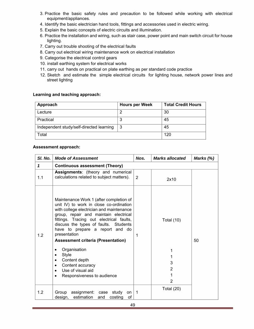
49
3. Practice the basic safety rules and precaution to be followed while working with electrical equipment/appliances.
4. Identify the basic electrician hand tools, fittings and accessories used in electric wiring. 5. Explain the basic concepts of electric circuits and illumination. 6. Practice the installation and wiring, such as stair case, power point and main switch circuit for house
lighting. 7. Carry out trouble shooting of the electrical faults 8. Carry out electrical wiring maintenance work on electrical installation 9. Categorise the electrical control gears 10. install earthing system for electrical works 11. carry out hands on practical on plate earthing as per standard code practice 12. Sketch and estimate the simple electrical circuits for lighting house, network power lines and
street lighting
Learning and teaching approach:
Approach Hours per Week Total Credit Hours
Lecture 2 30
Practical 3 45
Independent study/self-directed learning 3 45
Total 120
Assessment approach:
Sl. No. Mode of Assessment Nos. Marks allocated Marks (%)
1 Continuous assessment (Theory)
1.1 Assignments: (theory and numerical calculations related to subject matters).
2
2x10
50 1.2
Maintenance Work 1 (after completion of unit IV) to work in close co-ordination with college electrician and maintenance group, repair and maintain electrical fittings. Tracing out electrical faults, discuss the types of faults. Students have to prepare a report and do presentation
Assessment criteria (Presentation)
Organisation Style Content depth Content accuracy Use of visual aid Responsiveness to audience
1
Total (10)
1
1
3
2
1
2
1.2 Group assignment: case study on design, estimation and costing of
1 Total (20)
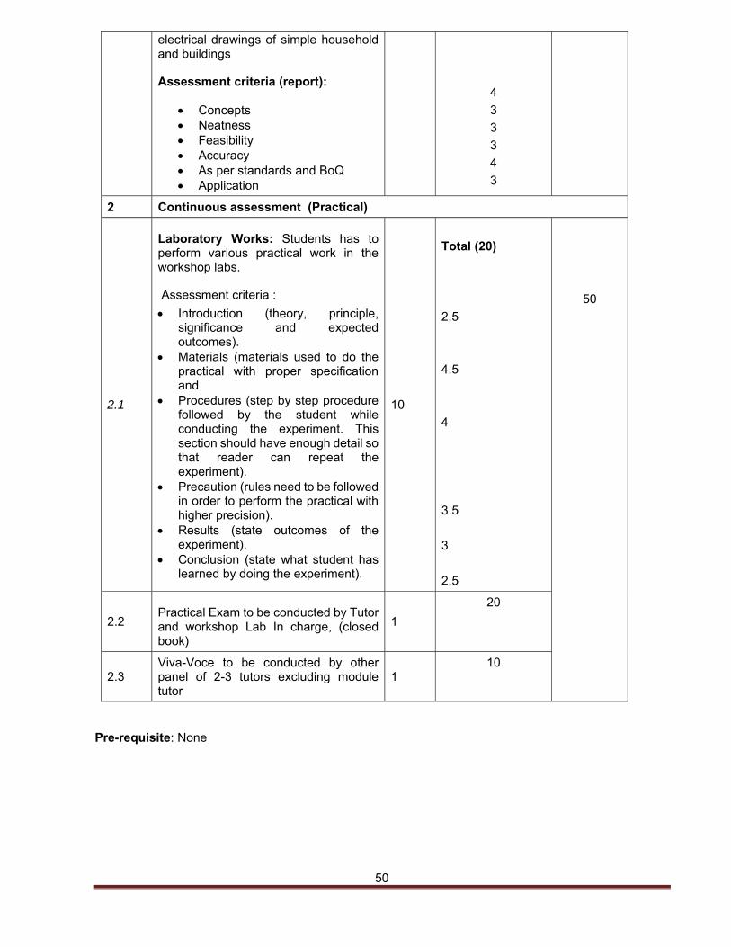
50
electrical drawings of simple household and buildings
Assessment criteria (report):
Concepts Neatness Feasibility Accuracy As per standards and BoQ Application
4
3
3
3
4
3
2 Continuous assessment (Practical)
2.1
Laboratory Works: Students has to perform various practical work in the workshop labs.
Assessment criteria :
Introduction (theory, principle, significance and expected outcomes).
Materials (materials used to do the practical with proper specification and
Procedures (step by step procedure followed by the student while conducting the experiment. This section should have enough detail so that reader can repeat the experiment).
Precaution (rules need to be followed in order to perform the practical with higher precision).
Results (state outcomes of the experiment).
Conclusion (state what student has learned by doing the experiment).
10
Total (20)
2.5
4.5
4
3.5
3
2.5
50
2.2 Practical Exam to be conducted by Tutor and workshop Lab In charge, (closed book)
1
20
2.3 Viva-Voce to be conducted by other panel of 2-3 tutors excluding module tutor
1 10
Pre-requisite: None
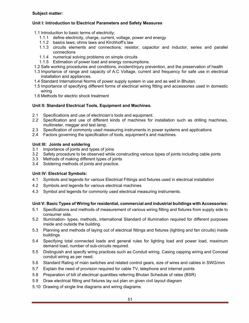
51
Subject matter: Unit I: Introduction to Electrical Parameters and Safety Measures 1.1 Introduction to basic terms of electricity;
1.1.1 define electricity, charge, current, voltage, power and energy 1.1.2 basics laws; ohms laws and Kirchhoff’s law 1.1.3 circuits elements and connections; resistor, capacitor and inductor, series and parallel
connections 1.1.4 numerical solving problems on simple circuits 1.1.5 Estimation of power load and energy consumptions.
1.2 Safe working procedures and conditions, incident/injury prevention, and the preservation of health 1.3 Importance of range and capacity of A.C Voltage, current and frequency for safe use in electrical
installation and appliances. 1.4 Standard International Norms of power supply system in use and as well in Bhutan. 1.5 Importance of specifying different forms of electrical wiring fitting and accessories used in domestic
wiring 1.6 Methods for electric shock treatment
Unit II: Standard Electrical Tools, Equipment and Machines. 2.1 Specifications and use of electrician’s tools and equipment. 2.2 Specification and use of different kinds of machines for installation such as drilling machines,
multimeter, meggar and test lamp. 2.3 Specification of commonly used measuring instruments in power systems and applications 2.4 Factors governing the specification of tools, equipment’s and machines. Unit III: Joints and soldering 3.1 Importance of joints and types of joins 3.2 Safety procedure to be observed while constructing various types of joints including cable joints 3.3 Methods of making different types of joints 3.4 Soldering methods of joints and practice. Unit IV: Electrical Symbols:
4.1 Symbols and legends for various Electrical Fittings and fixtures used in electrical installation
4.2 Symbols and legends for various electrical machines
4.3 Symbol and legends for commonly used electrical measuring instruments.
Unit V: Basic Types of Wiring for residential, commercial and industrial buildings with Accessories:
5.1 Specifications and methods of measurement of various wiring fitting and fixtures from supply side to consumer side.
5.2 Illumination- types, methods, international Standard of illumination required for different purposes inside and outside the building.
5.3 Planning and methods of laying out of electrical fittings and fixtures (lighting and fan circuits) inside buildings
5.4 Specifying total connected loads and general rules for lighting load and power load, maximum demand load, number of sub-circuits required.
5.5 Distinguish and specify wring practices such as Conduit wiring, Casing capping wiring and Conceal conduit wiring as per need.
5.6 Standard Rating of main switches and related control gears, size of wires and cables in SWG/mm
5.7 Explain the need of provision required for cable TV, telephone and internet points
5.8 Preparation of bill of electrical quantities referring Bhutan Schedule of rates (BSR)
5.9 Draw electrical fitting and fixtures lay out plan on given civil layout diagram
5.10 Drawing of single line diagrams and wiring diagrams.
52
Unit VI: EARTHING
6.1 Importance of earthing
6.2 Factors affecting the earth resistance
6.3 System earthing and equipment earthing
6.4 Rod and strip earthing
6.5 Plate earthing and pipe earthing
6.6 Earth wires used in a residential wiring
6.7 Earth resistance for domestic wiring, machine installation and sub-station
6.8 Preparation of the bill of materials for plate earthing and pipe earthing
6.9 Specification, circuit and use of earth tester
Unit VII: MAINTENANCE OF WIRING INSTALLATION
7.1 Carrying out electrical maintenance as required, in close co-ordination with the electrical maintenance in-charge.
7.2 Discussion on nature of fault,
7.3 Tracing of electrical faults,
7.4 Faults in distribution network,
7.5 Maintenance work (find out the possible area in the campus).
List of Practical: 1. Identify and write down the specification of commonly used electrician’s tools, equipment, and Fittings. 2. Making of different types of joints 3. Perform soldering on joints and printed circuit board 4. Carry out, test and prepare BOQ for PVC Wiring and testing of electrical installation (from Main DB,
MCB-DB, ENERGY METER to Bus Bar Chamber ) 5. Carry out, test and prepare BOQ for two way switch wiring 6. Carry out, test and prepare BOQ for Power circuit wiring 7. Perform testing of Fluorescent lamp, frame connection system, choke and starter. 8. Demonstrate the assembly of ceiling fan and circuit connections. 9. Carryout the earthing test for existing earthing points as per standard code of practice and perform
earth resistance test. Reading list: Essential Reading 1. Uppal S.L and Laroia J.M (2008). Electrical Wiring, Estimating and Costing. New Delhi: Khana
Publishers 2. Singh Surjeet (2008). A Textbook of Electrical Design and Drawing. New Delhi: S.K Kataria and
Sons. 3. Singh R.P, (2010). Electrical Workshop: A textbook. New Delhi: I.K International Publishing
House Pvt Limited. 4. Ambrousius, L. (2015). AutoCAD 2015 and AutoCAD LT 2015 Bible. (1ed.). New Delhi; Wiley.
Additional Reading 1 Wadha, C. L. (2006). Generation, Distribution and Utilization of Electrical Energy, New Delhi, Wiley
Eastern Limited. 2 Bhatia, S. L. (2006). Handbook of Electrical Engineering. New Delhi; Khanna Publishers. 3 Raina, K.B. & Bhattacharya, S.K. (1991) Electrical Design, Estimating and Costing, (`1ed.). New
delhi; New Age International Publishers. 4 Anwani, M.L. (1972) Basic Electrical Engineering, (1ed.). New Delhi; Dhanpat rai & Co.(P)Ltd,
Educational and technical Publishers Date: 30thDecember, 2016
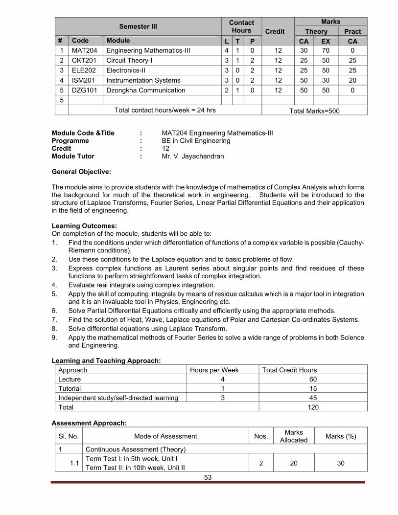
53
Semester III Contact Hours Credit
Marks
Theory Pract # Code Module L T P CA EX CA 1 MAT204 Engineering Mathematics-III 4 1 0 12 30 70 0
2 CKT201 Circuit Theory-I 3 1 2 12 25 50 25
3 ELE202 Electronics-II 3 0 2 12 25 50 25
4 ISM201 Instrumentation Systems 3 0 2 12 50 30 20
5 DZG101 Dzongkha Communication 2 1 0 12 50 50 0
5
Total contact hours/week = 24 hrs Total Marks=500
Module Code &Title : MAT204 Engineering Mathematics-III Programme : BE in Civil Engineering Credit : 12 Module Tutor : Mr. V. Jayachandran General Objective: The module aims to provide students with the knowledge of mathematics of Complex Analysis which forms the background for much of the theoretical work in engineering. Students will be introduced to the structure of Laplace Transforms, Fourier Series, Linear Partial Differential Equations and their application in the field of engineering. Learning Outcomes: On completion of the module, students will be able to: 1. Find the conditions under which differentiation of functions of a complex variable is possible (Cauchy-
Riemann conditions). 2. Use these conditions to the Laplace equation and to basic problems of flow. 3. Express complex functions as Laurent series about singular points and find residues of these
functions to perform straightforward tasks of complex integration. 4. Evaluate real integrals using complex integration. 5. Apply the skill of computing integrals by means of residue calculus which is a major tool in integration
and it is an invaluable tool in Physics, Engineering etc. 6. Solve Partial Differential Equations critically and efficiently using the appropriate methods. 7. Find the solution of Heat, Wave, Laplace equations of Polar and Cartesian Co-ordinates Systems. 8. Solve differential equations using Laplace Transform. 9. Apply the mathematical methods of Fourier Series to solve a wide range of problems in both Science
and Engineering. Learning and Teaching Approach:
Approach Hours per Week Total Credit Hours Lecture 4 60 Tutorial 1 15 Independent study/self-directed learning 3 45
Total 120 Assessment Approach:
Sl. No. Mode of Assessment Nos. Marks
Allocated Marks (%)
1 Continuous Assessment (Theory)
1.1 Term Test I: in 5th week, Unit I Term Test II: in 10th week, Unit II
2 20 30
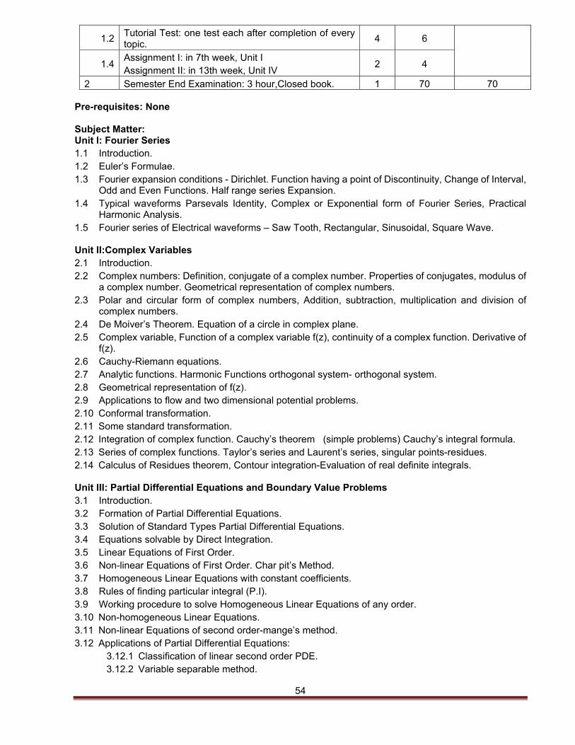
54
1.2 Tutorial Test: one test each after completion of every topic.
4 6
1.4 Assignment I: in 7th week, Unit I Assignment II: in 13th week, Unit IV
2 4
2 Semester End Examination: 3 hour,Closed book. 1 70 70 Pre-requisites: None Subject Matter: Unit I: Fourier Series 1.1 Introduction. 1.2 Euler’s Formulae. 1.3 Fourier expansion conditions - Dirichlet. Function having a point of Discontinuity, Change of Interval,
Odd and Even Functions. Half range series Expansion. 1.4 Typical waveforms Parsevals Identity, Complex or Exponential form of Fourier Series, Practical
Harmonic Analysis. 1.5 Fourier series of Electrical waveforms – Saw Tooth, Rectangular, Sinusoidal, Square Wave. Unit II:Complex Variables 2.1 Introduction. 2.2 Complex numbers: Definition, conjugate of a complex number. Properties of conjugates, modulus of
a complex number. Geometrical representation of complex numbers. 2.3 Polar and circular form of complex numbers, Addition, subtraction, multiplication and division of
complex numbers. 2.4 De Moiver’s Theorem. Equation of a circle in complex plane. 2.5 Complex variable, Function of a complex variable f(z), continuity of a complex function. Derivative of
f(z). 2.6 Cauchy-Riemann equations. 2.7 Analytic functions. Harmonic Functions orthogonal system- orthogonal system. 2.8 Geometrical representation of f(z). 2.9 Applications to flow and two dimensional potential problems. 2.10 Conformal transformation. 2.11 Some standard transformation. 2.12 Integration of complex function. Cauchy’s theorem (simple problems) Cauchy’s integral formula. 2.13 Series of complex functions. Taylor’s series and Laurent’s series, singular points-residues. 2.14 Calculus of Residues theorem, Contour integration-Evaluation of real definite integrals. Unit III: Partial Differential Equations and Boundary Value Problems 3.1 Introduction. 3.2 Formation of Partial Differential Equations. 3.3 Solution of Standard Types Partial Differential Equations. 3.4 Equations solvable by Direct Integration. 3.5 Linear Equations of First Order. 3.6 Non-linear Equations of First Order. Char pit’s Method. 3.7 Homogeneous Linear Equations with constant coefficients. 3.8 Rules of finding particular integral (P.I). 3.9 Working procedure to solve Homogeneous Linear Equations of any order. 3.10 Non-homogeneous Linear Equations. 3.11 Non-linear Equations of second order-mange’s method. 3.12 Applications of Partial Differential Equations:
3.12.1 Classification of linear second order PDE. 3.12.2 Variable separable method.
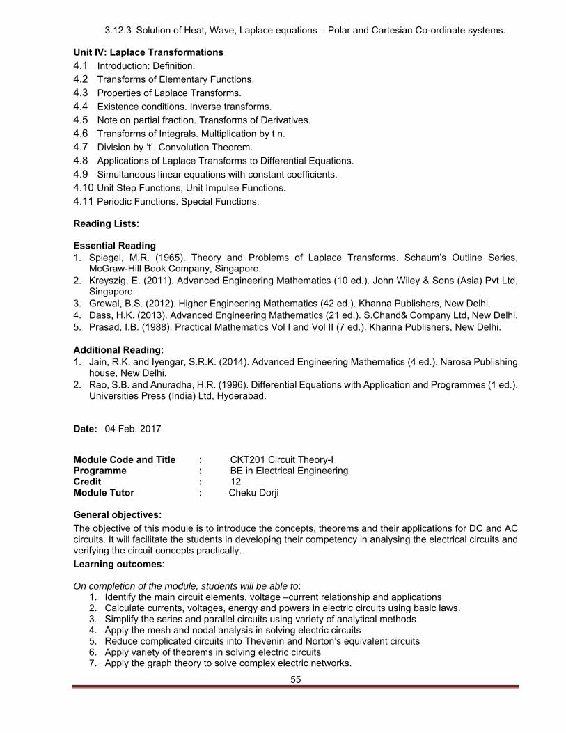
55
3.12.3 Solution of Heat, Wave, Laplace equations – Polar and Cartesian Co-ordinate systems. Unit IV: Laplace Transformations
4.1 Introduction: Definition.
4.2 Transforms of Elementary Functions.
4.3 Properties of Laplace Transforms.
4.4 Existence conditions. Inverse transforms.
4.5 Note on partial fraction. Transforms of Derivatives.
4.6 Transforms of Integrals. Multiplication by t n.
4.7 Division by ‘t’. Convolution Theorem.
4.8 Applications of Laplace Transforms to Differential Equations.
4.9 Simultaneous linear equations with constant coefficients.
4.10 Unit Step Functions, Unit Impulse Functions.
4.11 Periodic Functions. Special Functions. Reading Lists: Essential Reading 1. Spiegel, M.R. (1965). Theory and Problems of Laplace Transforms. Schaum’s Outline Series,
McGraw-Hill Book Company, Singapore. 2. Kreyszig, E. (2011). Advanced Engineering Mathematics (10 ed.). John Wiley & Sons (Asia) Pvt Ltd,
Singapore. 3. Grewal, B.S. (2012). Higher Engineering Mathematics (42 ed.). Khanna Publishers, New Delhi. 4. Dass, H.K. (2013). Advanced Engineering Mathematics (21 ed.). S.Chand& Company Ltd, New Delhi. 5. Prasad, I.B. (1988). Practical Mathematics Vol I and Vol II (7 ed.). Khanna Publishers, New Delhi.
Additional Reading: 1. Jain, R.K. and Iyengar, S.R.K. (2014). Advanced Engineering Mathematics (4 ed.). Narosa Publishing
house, New Delhi. 2. Rao, S.B. and Anuradha, H.R. (1996). Differential Equations with Application and Programmes (1 ed.).
Universities Press (India) Ltd, Hyderabad. Date: 04 Feb. 2017
Module Code and Title : CKT201 Circuit Theory-I Programme : BE in Electrical Engineering Credit : 12 Module Tutor : Cheku Dorji General objectives:
The objective of this module is to introduce the concepts, theorems and their applications for DC and AC circuits. It will facilitate the students in developing their competency in analysing the electrical circuits and verifying the circuit concepts practically.
Learning outcomes: On completion of the module, students will be able to:
1. Identify the main circuit elements, voltage –current relationship and applications 2. Calculate currents, voltages, energy and powers in electric circuits using basic laws. 3. Simplify the series and parallel circuits using variety of analytical methods 4. Apply the mesh and nodal analysis in solving electric circuits 5. Reduce complicated circuits into Thevenin and Norton’s equivalent circuits 6. Apply variety of theorems in solving electric circuits 7. Apply the graph theory to solve complex electric networks.
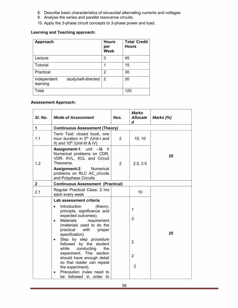
56
8. Describe basic characteristics of sinusoidal alternating currents and voltages 9. Analyse the series and parallel resonance circuits.
10. Apply the 3-phase circuit concepts to 3-phase power and load. Learning and Teaching approach:
Approach Hours per Week
Total Credit Hours
Lecture 3 45
Tutorial 1 15
Practical 2 30
Independent study/self-directed learning
2 30
Total 120
Assessment Approach:
Sl. No. Mode of Assessment Nos. Marks Allocated
Marks (%)
1 Continuous Assessment (Theory)
1.1 Term Test: closed book, one hour duration in 5th (Unit-I and II) and 10th (Unit-III & IV)
2 10, 10
25
1.2
Assignment-1: unit –I& II Numerical problems on CDR, VDR, KVL, KCL and Circuit Theorems.
Assignment-2: Numerical problems on RLC AC_circuits and Polyphase Circuits
2 2.5, 2.5
2 Continuous Assessment (Practical)
2.1 Regular Practical Class: 2 hrs each every week
10
25
Lab assessment criteria
Introduction (theory, principle, significance and expected outcomes).
Materials requirement (materials used to do the practical with proper specification)
Step by step procedure followed by the student while conducting the experiment. This section should have enough detail so that reader can repeat the experiment).
Precaution (rules need to be followed in order to
1
3
2
2
2
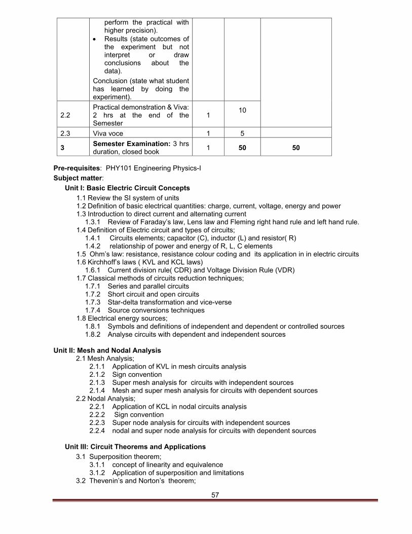
57
perform the practical with higher precision).
Results (state outcomes of the experiment but not interpret or draw conclusions about the data).
Conclusion (state what student has learned by doing the experiment).
2.2 Practical demonstration & Viva: 2 hrs at the end of the Semester
1 10
2.3 Viva voce 1 5
3 Semester Examination: 3 hrs duration, closed book
1 50 50
Pre-requisites: PHY101 Engineering Physics-I
Subject matter:
Unit I: Basic Electric Circuit Concepts
1.1 Review the SI system of units 1.2 Definition of basic electrical quantities: charge, current, voltage, energy and power 1.3 Introduction to direct current and alternating current
1.3.1 Review of Faraday’s law, Lens law and Fleming right hand rule and left hand rule. 1.4 Definition of Electric circuit and types of circuits;
1.4.1 Circuits elements; capacitor (C), inductor (L) and resistor( R) 1.4.2 relationship of power and energy of R, L, C elements
1.5 Ohm’s law: resistance, resistance colour coding and its application in in electric circuits 1.6 Kirchhoff’s laws ( KVL and KCL laws)
1.6.1 Current division rule( CDR) and Voltage Division Rule (VDR) 1.7 Classical methods of circuits reduction techniques;
1.7.1 Series and parallel circuits 1.7.2 Short circuit and open circuits 1.7.3 Star-delta transformation and vice-verse 1.7.4 Source conversions techniques
1.8 Electrical energy sources; 1.8.1 Symbols and definitions of independent and dependent or controlled sources 1.8.2 Analyse circuits with dependent and independent sources
Unit II: Mesh and Nodal Analysis
2.1 Mesh Analysis; 2.1.1 Application of KVL in mesh circuits analysis 2.1.2 Sign convention 2.1.3 Super mesh analysis for circuits with independent sources 2.1.4 Mesh and super mesh analysis for circuits with dependent sources
2.2 Nodal Analysis; 2.2.1 Application of KCL in nodal circuits analysis 2.2.2 Sign convention 2.2.3 Super node analysis for circuits with independent sources 2.2.4 nodal and super node analysis for circuits with dependent sources
Unit III: Circuit Theorems and Applications
3.1 Superposition theorem; 3.1.1 concept of linearity and equivalence 3.1.2 Application of superposition and limitations
3.2 Thevenin’s and Norton’s theorem;
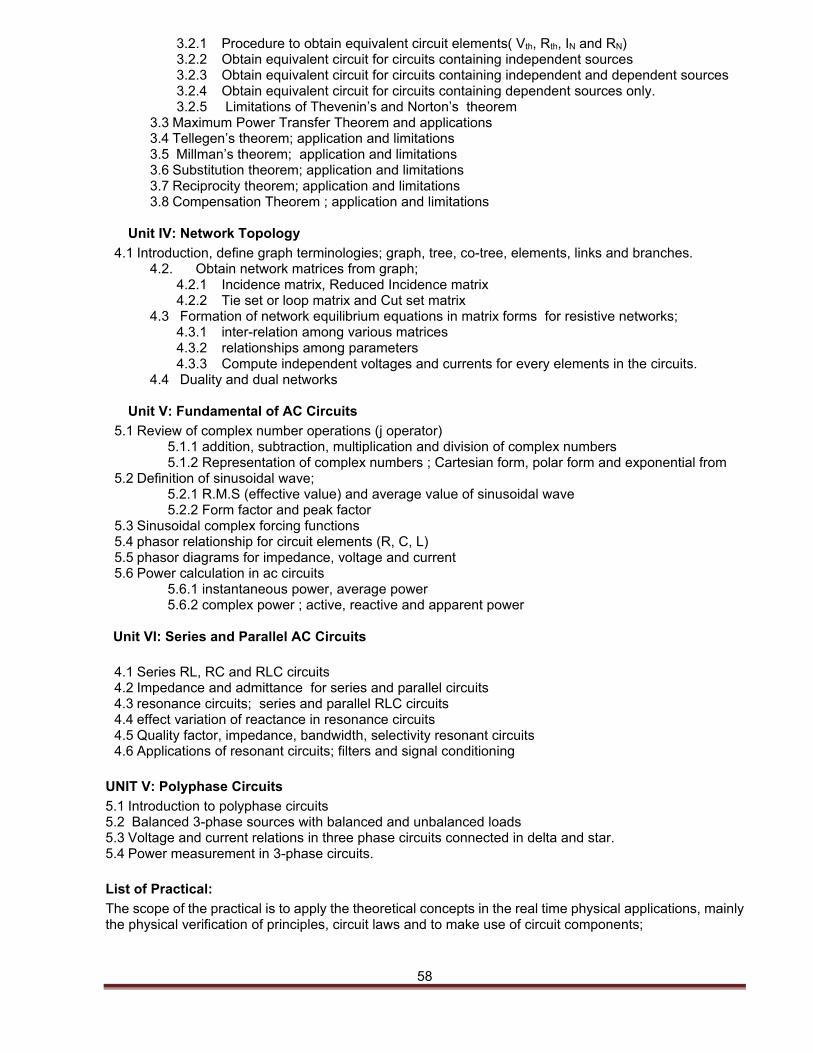
58
3.2.1 Procedure to obtain equivalent circuit elements( Vth, Rth, IN and RN) 3.2.2 Obtain equivalent circuit for circuits containing independent sources 3.2.3 Obtain equivalent circuit for circuits containing independent and dependent sources 3.2.4 Obtain equivalent circuit for circuits containing dependent sources only. 3.2.5 Limitations of Thevenin’s and Norton’s theorem
3.3 Maximum Power Transfer Theorem and applications 3.4 Tellegen’s theorem; application and limitations 3.5 Millman’s theorem; application and limitations 3.6 Substitution theorem; application and limitations 3.7 Reciprocity theorem; application and limitations 3.8 Compensation Theorem ; application and limitations
Unit IV: Network Topology
4.1 Introduction, define graph terminologies; graph, tree, co-tree, elements, links and branches. 4.2. Obtain network matrices from graph;
4.2.1 Incidence matrix, Reduced Incidence matrix 4.2.2 Tie set or loop matrix and Cut set matrix
4.3 Formation of network equilibrium equations in matrix forms for resistive networks; 4.3.1 inter-relation among various matrices 4.3.2 relationships among parameters 4.3.3 Compute independent voltages and currents for every elements in the circuits.
4.4 Duality and dual networks
Unit V: Fundamental of AC Circuits
5.1 Review of complex number operations (j operator) 5.1.1 addition, subtraction, multiplication and division of complex numbers 5.1.2 Representation of complex numbers ; Cartesian form, polar form and exponential from
5.2 Definition of sinusoidal wave; 5.2.1 R.M.S (effective value) and average value of sinusoidal wave 5.2.2 Form factor and peak factor
5.3 Sinusoidal complex forcing functions 5.4 phasor relationship for circuit elements (R, C, L) 5.5 phasor diagrams for impedance, voltage and current 5.6 Power calculation in ac circuits
5.6.1 instantaneous power, average power 5.6.2 complex power ; active, reactive and apparent power
Unit VI: Series and Parallel AC Circuits
4.1 Series RL, RC and RLC circuits 4.2 Impedance and admittance for series and parallel circuits 4.3 resonance circuits; series and parallel RLC circuits 4.4 effect variation of reactance in resonance circuits 4.5 Quality factor, impedance, bandwidth, selectivity resonant circuits 4.6 Applications of resonant circuits; filters and signal conditioning
UNIT V: Polyphase Circuits
5.1 Introduction to polyphase circuits 5.2 Balanced 3-phase sources with balanced and unbalanced loads 5.3 Voltage and current relations in three phase circuits connected in delta and star. 5.4 Power measurement in 3-phase circuits.
List of Practical:
The scope of the practical is to apply the theoretical concepts in the real time physical applications, mainly the physical verification of principles, circuit laws and to make use of circuit components;
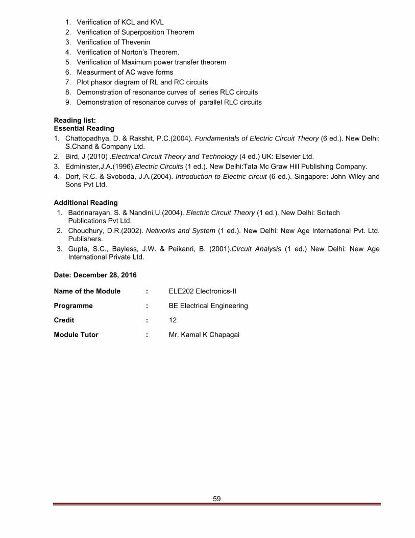
59
1. Verification of KCL and KVL
2. Verification of Superposition Theorem
3. Verification of Thevenin
4. Verification of Norton’s Theorem.
5. Verification of Maximum power transfer theorem
6. Measurment of AC wave forms
7. Plot phasor diagram of RL and RC circuits
8. Demonstration of resonance curves of series RLC circuits
9. Demonstration of resonance curves of parallel RLC circuits
Reading list: Essential Reading
1. Chattopadhya, D. & Rakshit, P.C.(2004). Fundamentals of Electric Circuit Theory (6 ed.). New Delhi: S.Chand & Company Ltd.
2. Bird, J (2010) .Electrical Circuit Theory and Technology (4 ed.) UK: Elsevier Ltd.
3. Edminister,J.A.(1996).Electric Circuits (1 ed.). New Delhi:Tata Mc Graw Hill Publishing Company.
4. Dorf, R.C. & Svoboda, J.A.(2004). Introduction to Electric circuit (6 ed.). Singapore: John Wiley and Sons Pvt Ltd.
Additional Reading
1. Badrinarayan, S. & Nandini,U.(2004). Electric Circuit Theory (1 ed.). New Delhi: Scitech Publications Pvt Ltd.
2. Choudhury, D.R.(2002). Networks and System (1 ed.). New Delhi: New Age International Pvt. Ltd. Publishers.
3. Gupta, S.C., Bayless, J.W. & Peikanri, B. (2001).Circuit Analysis (1 ed.) New Delhi: New Age International Private Ltd.
Date: December 28, 2016 Name of the Module : ELE202 Electronics-II
Programme : BE Electrical Engineering
Credit : 12
Module Tutor : Mr. Kamal K Chapagai
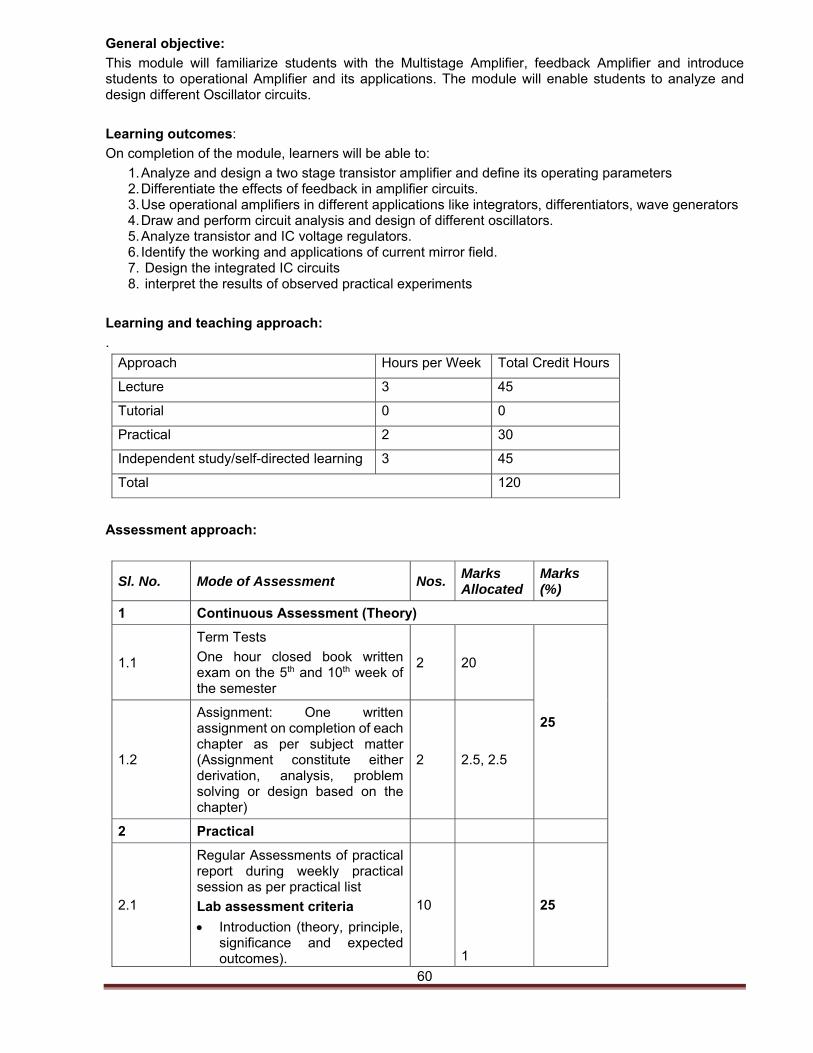
60
General objective:
This module will familiarize students with the Multistage Amplifier, feedback Amplifier and introduce students to operational Amplifier and its applications. The module will enable students to analyze and design different Oscillator circuits.
Learning outcomes:
On completion of the module, learners will be able to:
1. Analyze and design a two stage transistor amplifier and define its operating parameters 2. Differentiate the effects of feedback in amplifier circuits. 3. Use operational amplifiers in different applications like integrators, differentiators, wave generators 4. Draw and perform circuit analysis and design of different oscillators. 5. Analyze transistor and IC voltage regulators. 6. Identify the working and applications of current mirror field. 7. Design the integrated IC circuits 8. interpret the results of observed practical experiments
Learning and teaching approach:
.
Approach Hours per Week Total Credit Hours
Lecture 3 45
Tutorial 0 0
Practical 2 30
Independent study/self-directed learning 3 45
Total 120
Assessment approach:
Sl. No. Mode of Assessment Nos. Marks Allocated
Marks (%)
1 Continuous Assessment (Theory)
1.1
Term Tests
One hour closed book written exam on the 5th and 10th week of the semester
2 20
25
1.2
Assignment: One written assignment on completion of each chapter as per subject matter (Assignment constitute either derivation, analysis, problem solving or design based on the chapter)
2 2.5, 2.5
2 Practical
2.1
Regular Assessments of practical report during weekly practical session as per practical list
Lab assessment criteria
Introduction (theory, principle, significance and expected outcomes).
10
1
25
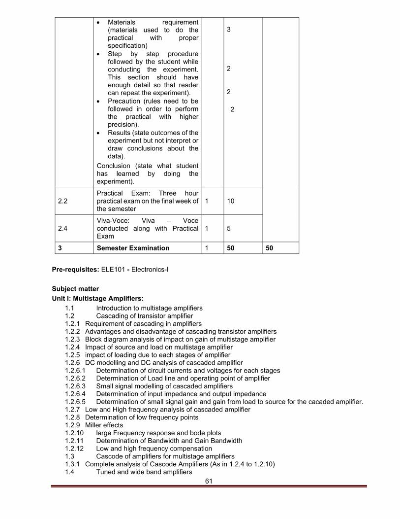
61
Materials requirement (materials used to do the practical with proper specification)
Step by step procedure followed by the student while conducting the experiment. This section should have enough detail so that reader can repeat the experiment).
Precaution (rules need to be followed in order to perform the practical with higher precision).
Results (state outcomes of the experiment but not interpret or draw conclusions about the data).
Conclusion (state what student has learned by doing the experiment).
3
2
2
2
2.2 Practical Exam: Three hour practical exam on the final week of the semester
1 10
2.4 Viva-Voce: Viva – Voce conducted along with Practical Exam
1 5
3 Semester Examination 1 50 50
Pre-requisites: ELE101 - Electronics-I
Subject matter
Unit I: Multistage Amplifiers:
1.1 Introduction to multistage amplifiers 1.2 Cascading of transistor amplifier 1.2.1 Requirement of cascading in amplifiers 1.2.2 Advantages and disadvantage of cascading transistor amplifiers 1.2.3 Block diagram analysis of impact on gain of multistage amplifier 1.2.4 Impact of source and load on multistage amplifier 1.2.5 impact of loading due to each stages of amplifier 1.2.6 DC modelling and DC analysis of cascaded amplifier 1.2.6.1 Determination of circuit currents and voltages for each stages 1.2.6.2 Determination of Load line and operating point of amplifier 1.2.6.3 Small signal modelling of cascaded amplifiers 1.2.6.4 Determination of input impedance and output impedance 1.2.6.5 Determination of small signal gain and gain from load to source for the cacaded amplifier. 1.2.7 Low and High frequency analysis of cascaded amplifier 1.2.8 Determination of low frequency points 1.2.9 Miller effects 1.2.10 large Frequency response and bode plots 1.2.11 Determination of Bandwidth and Gain Bandwidth 1.2.12 Low and high frequency compensation 1.3 Cascode of amplifiers for multistage amplifiers 1.3.1 Complete analysis of Cascode Amplifiers (As in 1.2.4 to 1.2.10) 1.4 Tuned and wide band amplifiers
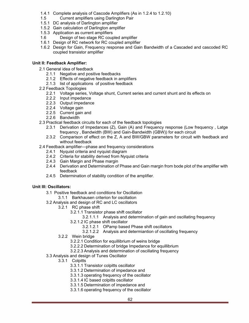
62
1.4.1 Complete analysis of Cascode Amplifiers (As in 1.2.4 to 1.2.10) 1.5 Current amplifiers using Darlington Pair 1.5.1 DC analysis of Darlington amplifier 1.5.2 Gain calculation of Darlington amplifier 1.5.3 Application as current amplifiers 1.6 Design of two stage RC coupled amplifier 1.6.1 Design of RC network for RC coupled amplifier 1.6.2 Design for Gain, Frequency response and Gain Bandwidth of a Cascaded and cascoded RC
coupled transistor amplifier
Unit II: Feedback Amplifier:
2.1 General idea of feedback 2.1.1 Negative and positive feedbacks 2.1.2 Effects of negative feedback in amplifiers 2.1.3 list of applications of positive feedback
2.2 Feedback Topologies 2.2.1 Voltage series, Voltage shunt, Current series and current shunt and its effects on 2.2.2 Input impedance 2.2.3 Output impedance 2.2.4 Voltage gain 2.2.5 Current gain and 2.2.6 Bandwidth
2.3 Practical feedback circuits for each of the feedback topologies 2.3.1 Derivation of Impedances (Z), Gain (A) and Frequency response (Low frequency , Latge
frequency , Bandwidth (BW) and Gain-Bandwidth (GBW)) for each circuit 2.3.2 Comparison of effect on the Z, A and BW/GBW parameters for circuit with feedback and
without feedback 2.4 Feedback amplifier—phase and frequency considerations
2.4.1 Nyquist criteria and nyquist diagram 2.4.2 Criteria for stability derived from Nyquist criteria 2.4.3 Gain Margin and Phase margin 2.4.4 Derivation and Determination of Phase and Gain margin from bode plot of the amplifier with
feedback 2.4.5 Determination of stability condition of the amplifier.
Unit III: Oscillators:
3.1 Positive feedback and conditions for Oscillation 3.1.1 Barkhausen criterion for oscillation
3.2 Analysis and design of RC and LC oscillators 3.2.1 RC phase shift
3.2.1.1 Transistor phase shift oscillator 3.2.1.1.1 Analysis and determination of gain and oscillating frequency
3.2.1.2 IC phase shift oscillator 3.2.1.2.1 OPamp based Phase shift oscillators 3.2.1.2.2 Analysis and determiantion of oscillating frequency
3.2.2 Wein bridge 3.2.2.1 Condition for equillibrium of weins bridge 3.2.2.2 Determination of bridge Impedance for equillibrium 3.2.2.3 Analysis and determination of oscillating frequency
3.3 Analysis and design of Tunes Oscillator 3.3.1 Colpitts
3.3.1.1 Transistor colpitts oscillator 3.3.1.2 Determination of impedance and 3.3.1.3 operating frequency of the oscillator 3.3.1.4 IC based colpitts oscillator 3.3.1.5 Determination of impedance and 3.3.1.6 operating frequency of the oscillator
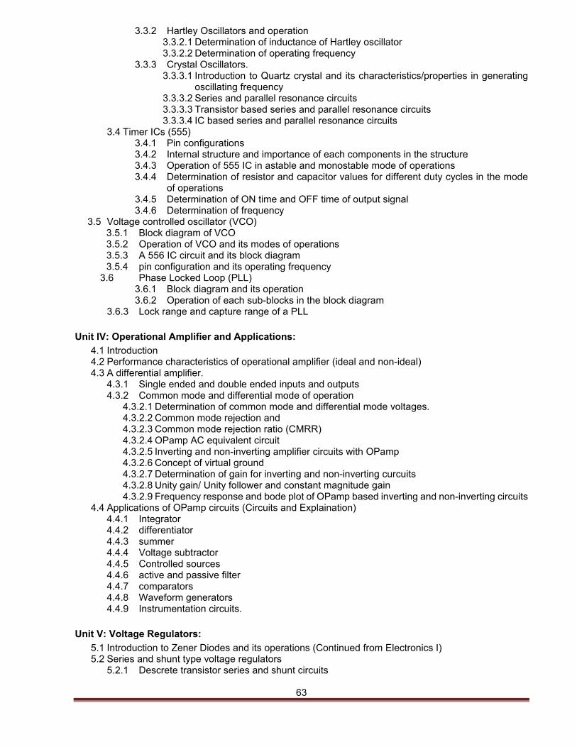
63
3.3.2 Hartley Oscillators and operation 3.3.2.1 Determination of inductance of Hartley oscillator 3.3.2.2 Determination of operating frequency
3.3.3 Crystal Oscillators. 3.3.3.1 Introduction to Quartz crystal and its characteristics/properties in generating
oscillating frequency 3.3.3.2 Series and parallel resonance circuits 3.3.3.3 Transistor based series and parallel resonance circuits 3.3.3.4 IC based series and parallel resonance circuits
3.4 Timer ICs (555) 3.4.1 Pin configurations 3.4.2 Internal structure and importance of each components in the structure 3.4.3 Operation of 555 IC in astable and monostable mode of operations 3.4.4 Determination of resistor and capacitor values for different duty cycles in the mode
of operations 3.4.5 Determination of ON time and OFF time of output signal 3.4.6 Determination of frequency
3.5 Voltage controlled oscillator (VCO) 3.5.1 Block diagram of VCO 3.5.2 Operation of VCO and its modes of operations 3.5.3 A 556 IC circuit and its block diagram 3.5.4 pin configuration and its operating frequency
3.6 Phase Locked Loop (PLL) 3.6.1 Block diagram and its operation 3.6.2 Operation of each sub-blocks in the block diagram
3.6.3 Lock range and capture range of a PLL
Unit IV: Operational Amplifier and Applications:
4.1 Introduction 4.2 Performance characteristics of operational amplifier (ideal and non-ideal) 4.3 A differential amplifier.
4.3.1 Single ended and double ended inputs and outputs 4.3.2 Common mode and differential mode of operation
4.3.2.1 Determination of common mode and differential mode voltages. 4.3.2.2 Common mode rejection and 4.3.2.3 Common mode rejection ratio (CMRR) 4.3.2.4 OPamp AC equivalent circuit 4.3.2.5 Inverting and non-inverting amplifier circuits with OPamp 4.3.2.6 Concept of virtual ground 4.3.2.7 Determination of gain for inverting and non-inverting curcuits 4.3.2.8 Unity gain/ Unity follower and constant magnitude gain 4.3.2.9 Frequency response and bode plot of OPamp based inverting and non-inverting circuits
4.4 Applications of OPamp circuits (Circuits and Explaination) 4.4.1 Integrator 4.4.2 differentiator 4.4.3 summer 4.4.4 Voltage subtractor 4.4.5 Controlled sources 4.4.6 active and passive filter 4.4.7 comparators 4.4.8 Waveform generators 4.4.9 Instrumentation circuits.
Unit V: Voltage Regulators:
5.1 Introduction to Zener Diodes and its operations (Continued from Electronics I) 5.2 Series and shunt type voltage regulators
5.2.1 Descrete transistor series and shunt circuits
64
5.2.2 Improved series and shunt regulators 5.2.3 OPamp/IC based series and shunt regulators 5.2.4 Determination of circuit currents and voltages 5.2.5 Determination of regulated voltages 5.2.6 Dependance of regulated voltages on circuit parameters
5.3 OL and SC protection 5.3.1 Transistorized current limiting circuits
5.4 IC/Three terminal voltage regulators 5.4.1 IC 78XX series 5.4.2 Operation and regulated voltages. 5.4.3 LM317 voltage regulator block and regulated voltage
Unit VI: Current Mirrors:
6.1 Introduction 6.2 Simple (basic) current mirror, working and applications
6.2.1 Simplified circuit of a BJT based current mirror 6.2.2 Explanation of the principle of current mirroring. 6.2.3 Calculation of the mirrored currents.
List of Practical:
Design and analysis of two stage RC coupled amplifiers
To study Series Current Feedback and to measure the voltage gains with and without bypass capacitor.
To construct an inverting and non-inverting amplifier using an OPAMP and perform the frequency analysis.
To study the application of Op Amp as Adder and Subtractor circuit.
To design and analyze a RC Phase shift oscillator with OPamp and determine the oscillating frequency
To design and analyze the operation of a 555 timer circuit in monostable and astable mode of operation and determine the rise time, fall time and frequency
Design and test a series voltage regulators using a transistor and Zener diode and detemine the regulated voltage.
Design and test a shunt voltage regulators using an OPamp and zenerdiode and detemine the regulated voltage.
Construct a simple current mirror using BJT and measure the currents flowing in the circuit.
Reading List Essential reading:
Jacob Millman and Christos C Halkias (2003), “Integrated Electronics, Analog and Digital circuits and Systems”, Tata McGraw Hill, New Delhi
Jacob Millman and Arvin Grabel, “Microelectronics”, McGraw Hill International Edn
Robert L Boyelstad and Louis Nashelsky (2001), “Electronics Devices and Circuit Theory”, 6th edition, PHI, New Delhi.
Muhammad H Rashid (1999), “Microelectronic Circuits: Analysis and Design”, 1st edition, PWS Publishing Company, Boston.
Additional reading:
1. Ramakant A Gayakwad (2002), “Op-Amp and Linear Integrated Circuits”, 4th edition, Pearson Education Asia, Singapore.
2. Malvino (1999), “Electronics Principles”, 6th edition, Tata McGraw Hill, New Delhi.
Date: 5th February 2016
65
Module Code and Title : ISM201 Instrumentation Systems
Programme : BE in Electrical Engineering
Credit : 12
Module Tutor : Tshewang Lhendup
General objectives:
This module will introduce various standards and unit systems used in measurements; various analog & digital instruments used for measurement of various electrical quantities and measurements applicable in electrical engineering.
Learning outcomes:
On completion of the module, students will be able to:
1. Explain the working principles of various measuring instruments.
2. Appraise the organization of instrumentation systems including the key elements.
3. Analyse uncertainties of the measuring instruments and measurement system.
4. Use ammeters, voltmeters and wattmeter to measure current, voltage and power.
5. Use bridges for measuring unknown inductance, capacitance, resistance, mutual inductance and frequency.
6. Analyse the construction and working principle of different types of ammeters, wattmeters, energy meters, maximum demand indicator and power factor meter.
7. Interpret the measured electrical parameters.
8. Differentiate different transducers and apply them for measuring a particular physical parameter
9. Use data loggers for recording time series data.
Learning and teaching approach:
Approach Hours per Week
Total Credit Hours
Lecture 3 45
Practical 2 30
Independent study/self-directed learning 3 45
Total 120
Assessment approach:
Sl. No. Mode of Assessment Nos. Marks Allocated
Marks (%)
1 Continuous Assessment (Theory)
1.1
Term Tests:Closed book, one hour duration in 5th and 10th week
Two units will be covered for term I and three units for term II.
2 10 20
66
Prerequisite: None
Subject matter:
Unit I: Standards of Measurement & Errors
1.1 Concept of generalized measurement system 1.2 Functional elements 1.3 Generalized input-output configuration 1.4 SI Units 1.5 Static & Dynamic characteristics of Electrical Instruments 1.6 Measurement errors and uncertainties.
Unit II: Electrical Instruments
1.2
Assignment: in 2nd week (Determining uncertainties of measuring instruments how it affects the parameter being measured. It will consists of ten numerical questions)
1 10
2 Continuous Assessment (Practical)
2.1
Regular Practical Class: 2 hrs each every week
Assessment will be based on report.
Identification of tools and equipment required and submission of requisition
Operational sequence (circuit diagram &circuit layout)
Procedure and precautions Observations and calculations
8
0.25
0.5
0.25
1.0
16
20
2.2 Practical demonstration: 2 hrs at the end of the Semester
1 4
3 Semester End Examination: 2 hrs duration, closed book
1 30 30
4
Project work (designing of data acquisition system. Students will have to design a complete data acquisition system using the transducers and instruments available in the lab. For example a home energy monitoring system using CT, voltage and current transducers)
Assessment Criteria (Report)
Introduction Principle of operation Feasibility of proposed system Design parameters Cost of proposed system Conclusions
Demonstration of system
Concepts Neatness Feasibility Presentation clarity As per standards and BoQ Application
1
30
10
1
2
2
2
2
1
(20)
3
3
3
5
3
3
30
67
2.1 Analog Electronic Instruments, Digital Instruments; Ammeters and Voltmeters;
Wattmeters
2.2 Measurement of active and reactive power with 2- wattmeter method
2.3 Energy meters for d.c. and a.c; Calibration of energy meters
2.4 Magnetic measurements; measurement of non-electrical quantities.
2.5 Special Meters - Maximum demand indicators, power factor meters for 1-phase and 3- phase system, synchroscopes, Megger, CRO and probes
2.6 Instrument transformers.
Unit III: Indicating Instruments
3.1 Galvanometers: Galvanometer equation in D.C. Measurements, D’Arsonval type, Vibration type and Balastic type.
3.2 Permanent magnet Moving coil (PMMC) Instrument
3.3 DC ammeters and voltmeters: construction and principle of operation.
Unit IV: RLC Measurement
4.1 D.C. and A.C Potentiometers, Polar and Coordinate A.C. Potentiometers,
Standardization, Basic concept of Self Balancing Potentiometer and its applications.
4.2 Measurement of low, medium and high resistances, insulation resistance of insulating
materials.
4.3 Bridges for inductance & mutual inductance measurement - Maxwell, Anderson, Hay,
Owen and Haviside Campbell bridges, Bridges for capacitance measurement - DeSauty,
Wien, Schering Bridge, Basic concept of Self Balancing Bridge and its applications.
Unit V: Magnetic Measurements
5.1 Purpose and methods of measurement, Choice of specimen and determination of
hysteresis loop, Permeability and iron loss measurement, A.C. magnetic measurement
Unit VI: Transducers
6.1 Terminology and definitions
6.2 Signal Conditioning and Processing
6.3 Electrical transducers for non-electrical quantities like length, displacement, velocity,
acceleration force, torque, level, pressure, temperature, flow, sound, light, humidity, and
pH; Pneumatic transducers for pressure, level temperature and flow; Actuators.
Unit VII: Instruments for Measuring Time, Frequency & Phase Angle
7.1 Time Measurement - Timing Marker, Analog electronic time interval meters
68
7.2 Frequency Measurement - CRO method, Heterodyne method; AC bridges for frequency measurement; analog electronic frequency meter
7.3 Phase Angle Measurement - CRO methods using single trace and dual trace CROs; Direct reading phase angle meters
Unit VIII: Analysers
8.1 Harmonic Distortion Analyser and Meter - Concept of Harmonic Distortion 8.2 Tuned circuit Harmonic Analyser, Heterodyne Harmonic distortion meter.
Unit IX: Introduction to Data recorders
9.1 Data loggers-types and functions
9.2 Online monitoring system-types and applications
List of Practicals:
1. Construct Owen’s Bridge and measure the unknown value of inductance.
2. Measurement of strain, pressure and speed.
3. Study characteristics of Thermocouples.
4. To measure active power, reactive power, apparent power using electronic power meter of different load.
5. Study the effect of introducing a measuring device into a circuit, and how the instrument affects the measurement.
6. Calibration of Energy Meter.
7. Harmonic distortion analyser.
8. Design instrumentation system.
Reading List:
Essential Reading
1. Sawhney, A. K. (2013). A course in Electrical and Electronic Measurement and Instrumentation (4 ed.). New Delhi: Dhanpat Rai and Sons.
2. Golding, E. W. (2012). Electrical Measurements and Measuring Instruments (6 ed.).New Delhi: A W Wheeler and Company Pvt. Ltd.
3. Deebelin, E. W. (2013). Measurement Systems: Applications and Design (4 ed). Singapore: McGraw Hill Book Co.
4. Norton, H. N. (2012). Handbook of Transducers for Electronic Measuring System (4 ed.). New Jersey: Prentice Hall Inc.
Additional Reading
1. Rangan, C. S., Sharma, C. R., & Mani, V.S. (2012). Instrumentation Devices and Systems (4 ed.). New Delhi: Tata McGraw Hill Pub. Co. Ltd.
2. Cooper, W. D., & Helfrick, A. D. (2011). Electronic Instrumentation and Measurement Techniques (5 ed.). New Delhi: Prentice Hall of India Pvt. Ltd.
3. Singh S. K. (2012). Industrial Instrumentation and Control (2 ed.). New Delhi: Tata McGraw Hill.
4. Oliver, B. M., & Cage, J. M. (2012). Electronic Measurement and Instrumentation (3 ed.). New York: McGraw Hill Koga Kusha Ltd.
5. Beerens, A. C. J. (2012). Measuring Methods and Devices in Electronics (4 ed.). New York: Haydess Book Co. Inc.
Date: 29 December, 2016
Semester IV Contact Hours
Credit Marks
Theory Pract
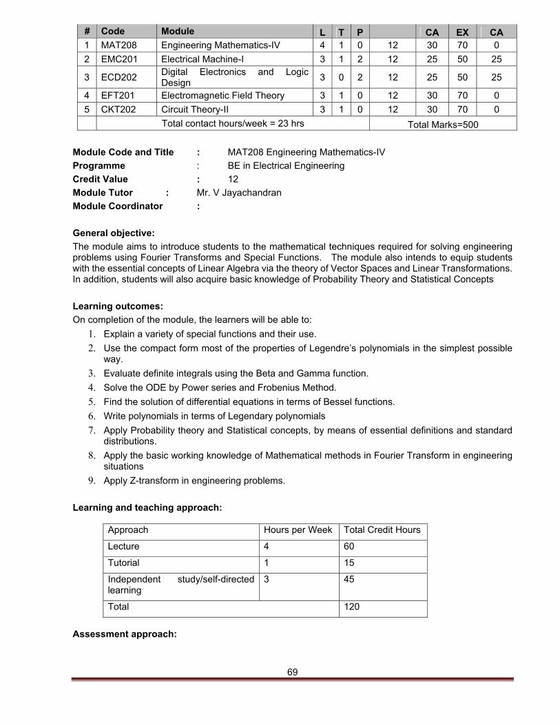
69
# Code Module L T P CA EX CA 1 MAT208 Engineering Mathematics-IV 4 1 0 12 30 70 0
2 EMC201 Electrical Machine-I 3 1 2 12 25 50 25
3 ECD202 Digital Electronics and Logic Design
3 0 2 12 25 50 25
4 EFT201 Electromagnetic Field Theory 3 1 0 12 30 70 0
5 CKT202 Circuit Theory-II 3 1 0 12 30 70 0
Total contact hours/week = 23 hrs Total Marks=500
Module Code and Title : MAT208 Engineering Mathematics-IV
Programme : BE in Electrical Engineering
Credit Value : 12
Module Tutor : Mr. V Jayachandran
Module Coordinator :
General objective:
The module aims to introduce students to the mathematical techniques required for solving engineering problems using Fourier Transforms and Special Functions. The module also intends to equip students with the essential concepts of Linear Algebra via the theory of Vector Spaces and Linear Transformations. In addition, students will also acquire basic knowledge of Probability Theory and Statistical Concepts
Learning outcomes:
On completion of the module, the learners will be able to:
1. Explain a variety of special functions and their use.
2. Use the compact form most of the properties of Legendre’s polynomials in the simplest possible way.
3. Evaluate definite integrals using the Beta and Gamma function.
4. Solve the ODE by Power series and Frobenius Method.
5. Find the solution of differential equations in terms of Bessel functions.
6. Write polynomials in terms of Legendary polynomials
7. Apply Probability theory and Statistical concepts, by means of essential definitions and standard distributions.
8. Apply the basic working knowledge of Mathematical methods in Fourier Transform in engineering situations
9. Apply Z-transform in engineering problems.
Learning and teaching approach:
Approach Hours per Week Total Credit Hours
Lecture 4 60
Tutorial 1 15
Independent study/self-directed learning
3 45
Total 120
Assessment approach:
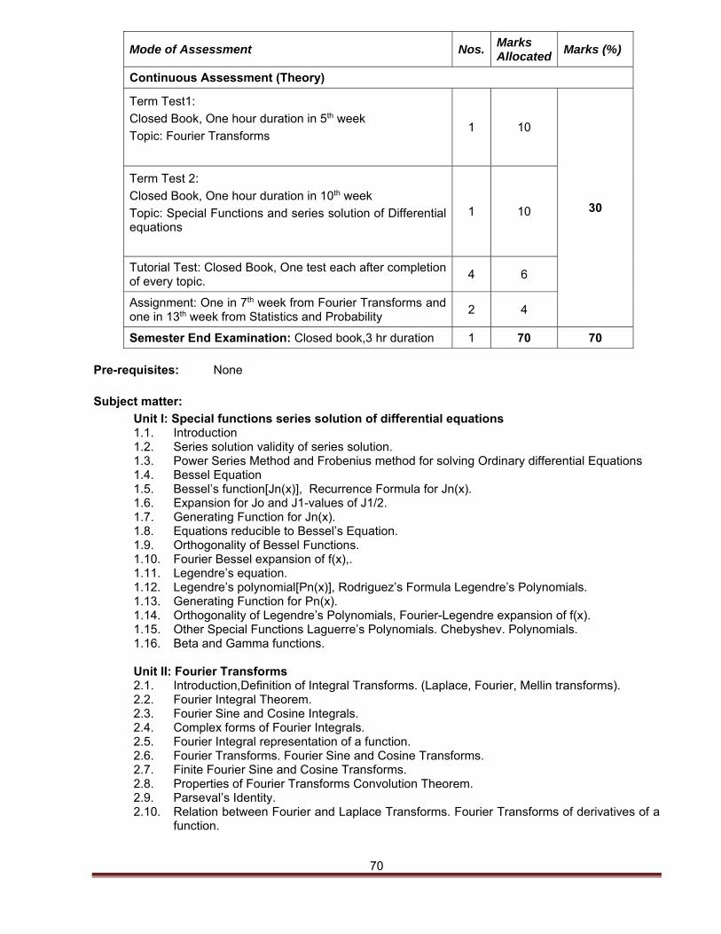
70
Mode of Assessment Nos.Marks Allocated
Marks (%)
Continuous Assessment (Theory)
Term Test1:
Closed Book, One hour duration in 5th week
Topic: Fourier Transforms
1 10
30
Term Test 2:
Closed Book, One hour duration in 10th week
Topic: Special Functions and series solution of Differential equations
1 10
Tutorial Test: Closed Book, One test each after completion of every topic.
4 6
Assignment: One in 7th week from Fourier Transforms and one in 13th week from Statistics and Probability
2 4
Semester End Examination: Closed book,3 hr duration 1 70 70
Pre-requisites: None
Subject matter:
Unit I: Special functions series solution of differential equations 1.1. Introduction 1.2. Series solution validity of series solution. 1.3. Power Series Method and Frobenius method for solving Ordinary differential Equations 1.4. Bessel Equation 1.5. Bessel’s function[Jn(x)], Recurrence Formula for Jn(x). 1.6. Expansion for Jo and J1-values of J1/2. 1.7. Generating Function for Jn(x). 1.8. Equations reducible to Bessel’s Equation. 1.9. Orthogonality of Bessel Functions. 1.10. Fourier Bessel expansion of f(x),. 1.11. Legendre’s equation. 1.12. Legendre’s polynomial[Pn(x)], Rodriguez’s Formula Legendre’s Polynomials. 1.13. Generating Function for Pn(x). 1.14. Orthogonality of Legendre’s Polynomials, Fourier-Legendre expansion of f(x). 1.15. Other Special Functions Laguerre’s Polynomials. Chebyshev. Polynomials. 1.16. Beta and Gamma functions.
Unit II: Fourier Transforms 2.1. Introduction,Definition of Integral Transforms. (Laplace, Fourier, Mellin transforms). 2.2. Fourier Integral Theorem. 2.3. Fourier Sine and Cosine Integrals. 2.4. Complex forms of Fourier Integrals. 2.5. Fourier Integral representation of a function. 2.6. Fourier Transforms. Fourier Sine and Cosine Transforms. 2.7. Finite Fourier Sine and Cosine Transforms. 2.8. Properties of Fourier Transforms Convolution Theorem. 2.9. Parseval’s Identity. 2.10. Relation between Fourier and Laplace Transforms. Fourier Transforms of derivatives of a
function.
71
Unit III: Z-Transforms 3.1. Definition 3.2. Standard Z-Transforms 3.3. Damping Rule 3.4. Change of scale and shifting property 3.5. Multiplication and division by K 3.6. Inverse z-transforms, 3.7. Inverse Z-Transforms by method of Residues 3.8. Convolution Theorem 3.9. Convergence of Z-transforms and application to Differential Equation.
Unit IV: Statistics and Probability 4.1. Measures of central tendency 4.2. Measures of Dispersion 4.3. Correlation(including Rank correlation) and regression 4.4. Sample Spaces 4.5. Axioms of Probability 4.6. Conditional Probability 4.7. Standard Distributions and z-Distribution 4.8. Joint Probability Distributions 4.9. Sampling Distributions 4.10. Point and Interval Estimation
Reading List:
Essential Reading
1. Kreyszig, E (2011), “Advanced Engineering Mathematics”, 10th edition, John Wiley & Sons (Asia) Pvt Ltd, Singapore
2. Dr. Grewal, B.S. (2007) “Higher Engineering Mathematics”, 40th edition,New Delhi: Khanna Publishers.
3. Dass, H.K (2013), “Advanced Engineering Mathematics”, 21st edition, S.Chand & Company Ltd, New Delhi.
4. Jain, R.K. and Iyengar S.R.K(2002). “Advanced Engineering Mathematics”. New Delhi: New Age International.
Additional Reading
1. Balachandra Rao, S. and Anuradha, H.R.(2008) “Differential Equations with Application and Programmes”.
2. Miller and John, E. F (2016), “Probability & Statistics for Engineers”, 9th Edition, Prentice Hall of India.
3. Iyengar, T.K.V and Gandhi, B.K., Probability & Statistics, S.Chand & Company
Date: 4 Feb, 2017
Module Code and Title : EMC201 Electrical Machine -I
Programme : B.E. in Electrical Engineering
Credit : 12
Module Tutor : Mr. Prem Kumar Nepal
General objectives or aims of the module:
The objective of the module is to introduce the physical construction, working principles and practical concepts of D.C. machines, transformers and their applications.
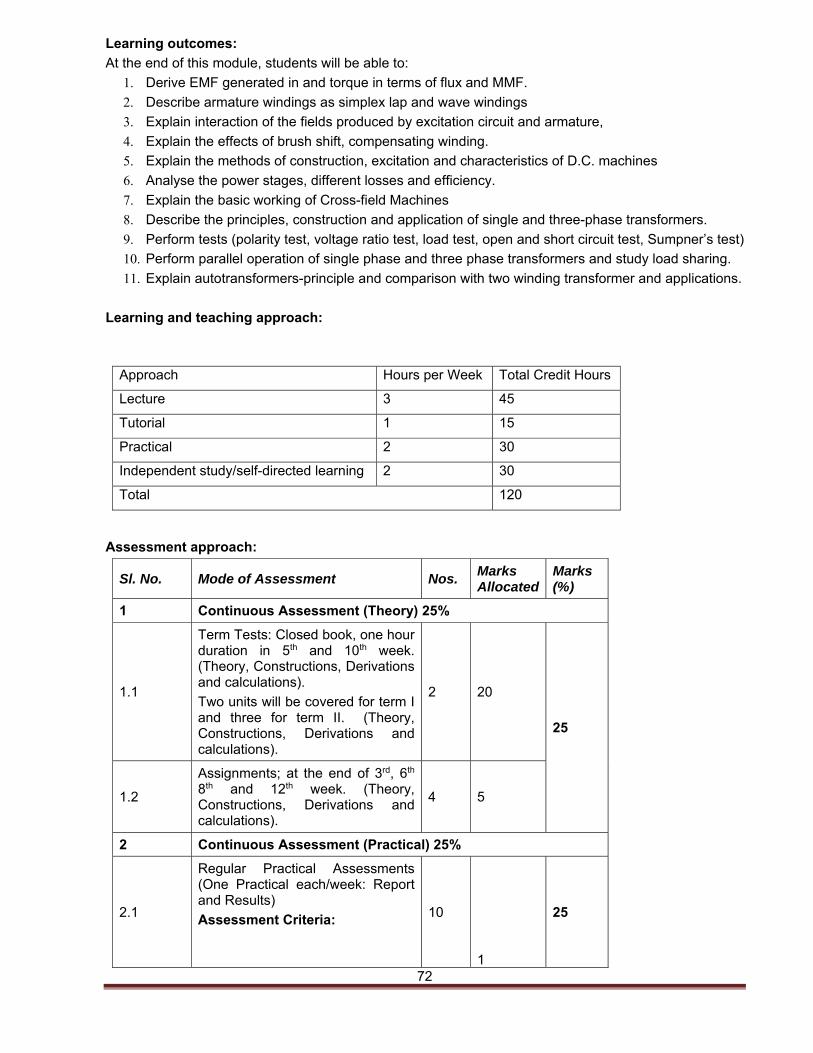
72
Learning outcomes:
At the end of this module, students will be able to:
1. Derive EMF generated in and torque in terms of flux and MMF.
2. Describe armature windings as simplex lap and wave windings
3. Explain interaction of the fields produced by excitation circuit and armature,
4. Explain the effects of brush shift, compensating winding.
5. Explain the methods of construction, excitation and characteristics of D.C. machines
6. Analyse the power stages, different losses and efficiency.
7. Explain the basic working of Cross-field Machines
8. Describe the principles, construction and application of single and three-phase transformers.
9. Perform tests (polarity test, voltage ratio test, load test, open and short circuit test, Sumpner’s test)
10. Perform parallel operation of single phase and three phase transformers and study load sharing.
11. Explain autotransformers-principle and comparison with two winding transformer and applications.
Learning and teaching approach:
Approach Hours per Week Total Credit Hours
Lecture 3 45
Tutorial 1 15
Practical 2 30
Independent study/self-directed learning 2 30
Total 120
Assessment approach:
Sl. No. Mode of Assessment Nos. Marks Allocated
Marks (%)
1 Continuous Assessment (Theory) 25%
1.1
Term Tests: Closed book, one hour duration in 5th and 10th week. (Theory, Constructions, Derivations and calculations).
Two units will be covered for term I and three for term II. (Theory, Constructions, Derivations and calculations).
2 20
25
1.2
Assignments; at the end of 3rd, 6th 8th and 12th week. (Theory, Constructions, Derivations and calculations).
4 5
2 Continuous Assessment (Practical) 25%
2.1
Regular Practical Assessments (One Practical each/week: Report and Results)
Assessment Criteria: 10
1
25
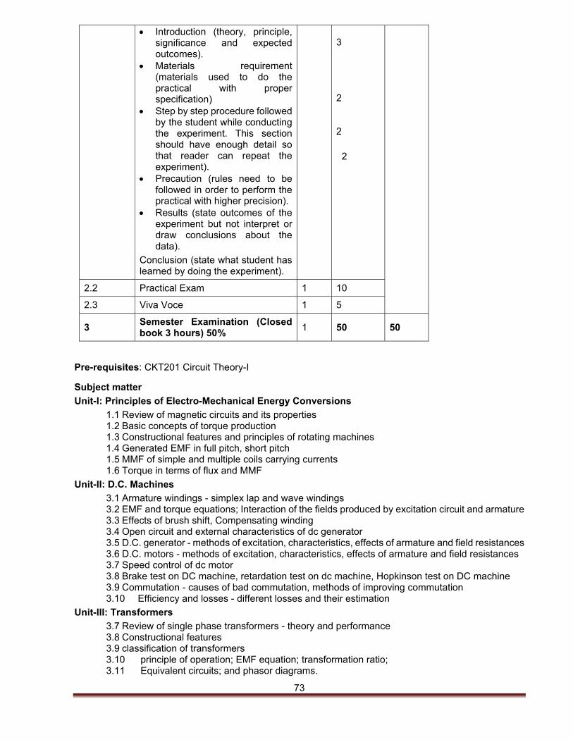
73
Introduction (theory, principle, significance and expected outcomes).
Materials requirement (materials used to do the practical with proper specification)
Step by step procedure followed by the student while conducting the experiment. This section should have enough detail so that reader can repeat the experiment).
Precaution (rules need to be followed in order to perform the practical with higher precision).
Results (state outcomes of the experiment but not interpret or draw conclusions about the data).
Conclusion (state what student has learned by doing the experiment).
3
2
2
2
2.2 Practical Exam 1 10
2.3 Viva Voce 1 5
3 Semester Examination (Closed book 3 hours) 50%
1 50 50
Pre-requisites: CKT201 Circuit Theory-I
Subject matter
Unit-I: Principles of Electro-Mechanical Energy Conversions
1.1 Review of magnetic circuits and its properties 1.2 Basic concepts of torque production 1.3 Constructional features and principles of rotating machines 1.4 Generated EMF in full pitch, short pitch 1.5 MMF of simple and multiple coils carrying currents 1.6 Torque in terms of flux and MMF
Unit-II: D.C. Machines
3.1 Armature windings - simplex lap and wave windings 3.2 EMF and torque equations; Interaction of the fields produced by excitation circuit and armature 3.3 Effects of brush shift, Compensating winding 3.4 Open circuit and external characteristics of dc generator 3.5 D.C. generator - methods of excitation, characteristics, effects of armature and field resistances 3.6 D.C. motors - methods of excitation, characteristics, effects of armature and field resistances 3.7 Speed control of dc motor 3.8 Brake test on DC machine, retardation test on dc machine, Hopkinson test on DC machine 3.9 Commutation - causes of bad commutation, methods of improving commutation 3.10 Efficiency and losses - different losses and their estimation
Unit-III: Transformers
3.7 Review of single phase transformers - theory and performance 3.8 Constructional features 3.9 classification of transformers 3.10 principle of operation; EMF equation; transformation ratio; 3.11 Equivalent circuits; and phasor diagrams.
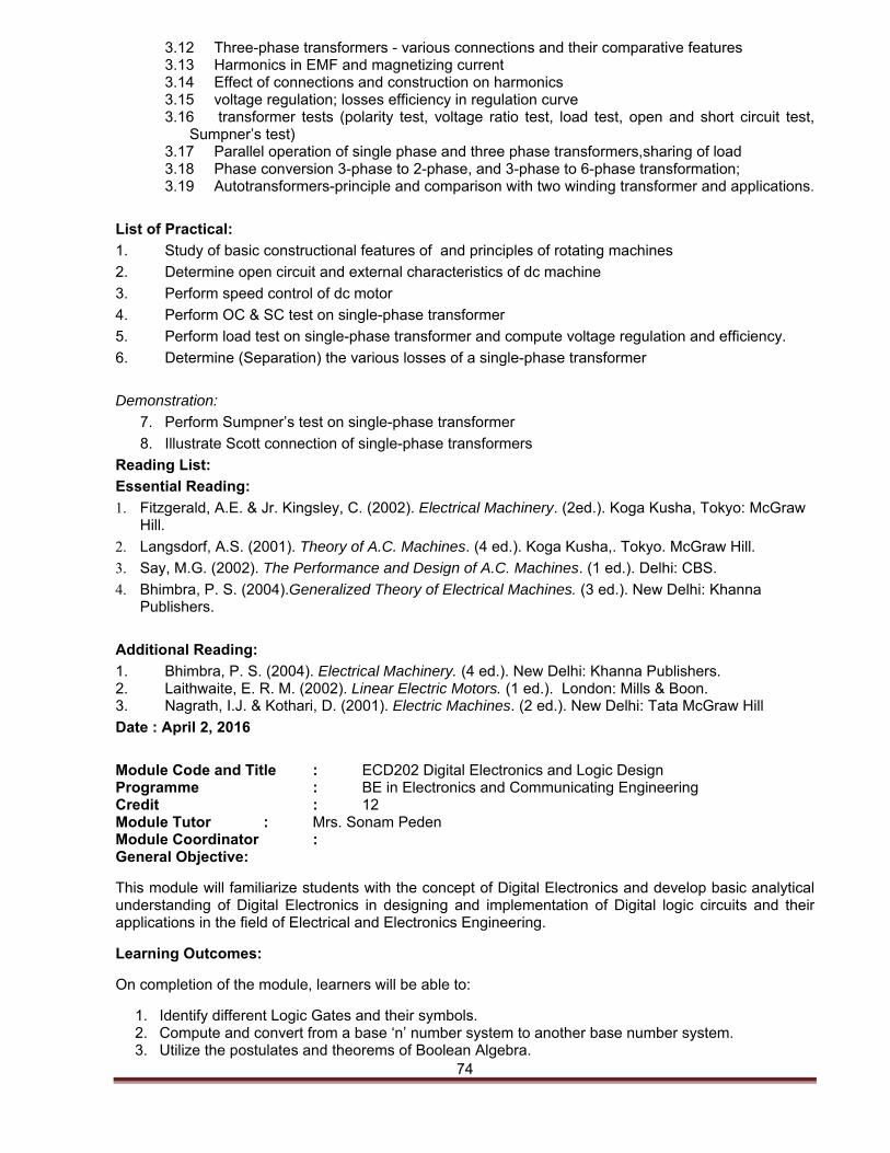
74
3.12 Three-phase transformers - various connections and their comparative features 3.13 Harmonics in EMF and magnetizing current 3.14 Effect of connections and construction on harmonics 3.15 voltage regulation; losses efficiency in regulation curve 3.16 transformer tests (polarity test, voltage ratio test, load test, open and short circuit test,
Sumpner’s test) 3.17 Parallel operation of single phase and three phase transformers,sharing of load 3.18 Phase conversion 3-phase to 2-phase, and 3-phase to 6-phase transformation; 3.19 Autotransformers-principle and comparison with two winding transformer and applications.
List of Practical:
1. Study of basic constructional features of and principles of rotating machines
2. Determine open circuit and external characteristics of dc machine
3. Perform speed control of dc motor
4. Perform OC & SC test on single-phase transformer
5. Perform load test on single-phase transformer and compute voltage regulation and efficiency.
6. Determine (Separation) the various losses of a single-phase transformer
Demonstration:
7. Perform Sumpner’s test on single-phase transformer
8. Illustrate Scott connection of single-phase transformers
Reading List:
Essential Reading:
1. Fitzgerald, A.E. & Jr. Kingsley, C. (2002). Electrical Machinery. (2ed.). Koga Kusha, Tokyo: McGraw Hill.
2. Langsdorf, A.S. (2001). Theory of A.C. Machines. (4 ed.). Koga Kusha,. Tokyo. McGraw Hill.
3. Say, M.G. (2002). The Performance and Design of A.C. Machines. (1 ed.). Delhi: CBS.
4. Bhimbra, P. S. (2004).Generalized Theory of Electrical Machines. (3 ed.). New Delhi: Khanna Publishers.
Additional Reading:
1. Bhimbra, P. S. (2004). Electrical Machinery. (4 ed.). New Delhi: Khanna Publishers. 2. Laithwaite, E. R. M. (2002). Linear Electric Motors. (1 ed.). London: Mills & Boon. 3. Nagrath, I.J. & Kothari, D. (2001). Electric Machines. (2 ed.). New Delhi: Tata McGraw Hill
Date : April 2, 2016
Module Code and Title : ECD202 Digital Electronics and Logic Design Programme : BE in Electronics and Communicating Engineering Credit : 12 Module Tutor : Mrs. Sonam Peden Module Coordinator : General Objective:
This module will familiarize students with the concept of Digital Electronics and develop basic analytical understanding of Digital Electronics in designing and implementation of Digital logic circuits and their applications in the field of Electrical and Electronics Engineering.
Learning Outcomes:
On completion of the module, learners will be able to:
1. Identify different Logic Gates and their symbols. 2. Compute and convert from a base ‘n’ number system to another base number system. 3. Utilize the postulates and theorems of Boolean Algebra.
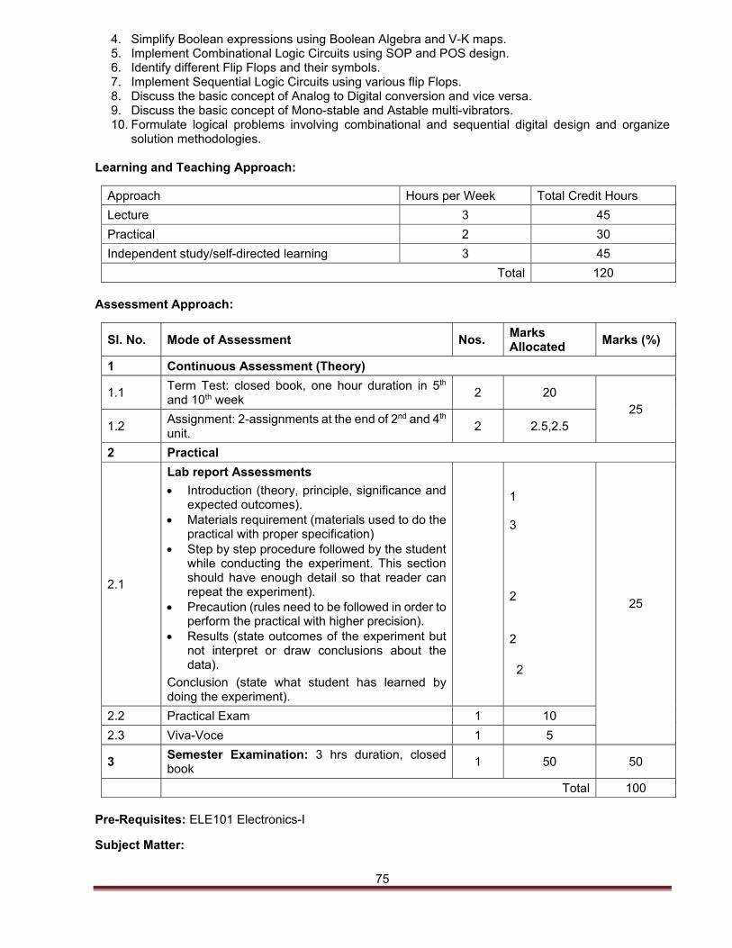
75
4. Simplify Boolean expressions using Boolean Algebra and V-K maps. 5. Implement Combinational Logic Circuits using SOP and POS design. 6. Identify different Flip Flops and their symbols. 7. Implement Sequential Logic Circuits using various flip Flops. 8. Discuss the basic concept of Analog to Digital conversion and vice versa. 9. Discuss the basic concept of Mono-stable and Astable multi-vibrators. 10. Formulate logical problems involving combinational and sequential digital design and organize
solution methodologies. Learning and Teaching Approach:
Approach Hours per Week Total Credit Hours
Lecture 3 45
Practical 2 30
Independent study/self-directed learning 3 45
Total 120 Assessment Approach:
Sl. No. Mode of Assessment Nos. Marks Allocated
Marks (%)
1 Continuous Assessment (Theory)
1.1 Term Test: closed book, one hour duration in 5th and 10th week
2 20 25
1.2 Assignment: 2-assignments at the end of 2nd and 4th unit.
2 2.5,2.5
2 Practical
2.1
Lab report Assessments
Introduction (theory, principle, significance and expected outcomes).
Materials requirement (materials used to do the practical with proper specification)
Step by step procedure followed by the student while conducting the experiment. This section should have enough detail so that reader can repeat the experiment).
Precaution (rules need to be followed in order to perform the practical with higher precision).
Results (state outcomes of the experiment but not interpret or draw conclusions about the data).
Conclusion (state what student has learned by doing the experiment).
1
3
2
2 2
25
2.2 Practical Exam 1 10
2.3 Viva-Voce 1 5
3 Semester Examination: 3 hrs duration, closed book
1 50 50
Total 100 Pre-Requisites: ELE101 Electronics-I
Subject Matter:
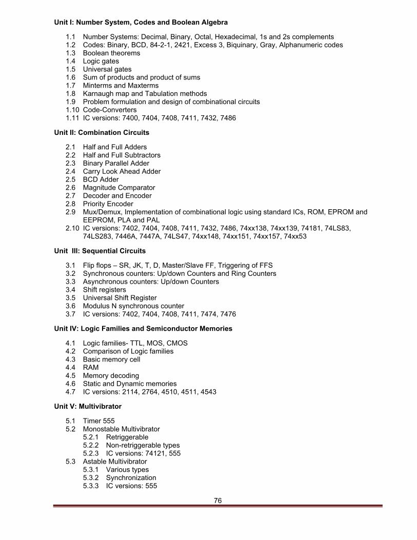
76
Unit I: Number System, Codes and Boolean Algebra
1.1 Number Systems: Decimal, Binary, Octal, Hexadecimal, 1s and 2s complements 1.2 Codes: Binary, BCD, 84-2-1, 2421, Excess 3, Biquinary, Gray, Alphanumeric codes 1.3 Boolean theorems 1.4 Logic gates 1.5 Universal gates 1.6 Sum of products and product of sums 1.7 Minterms and Maxterms 1.8 Karnaugh map and Tabulation methods 1.9 Problem formulation and design of combinational circuits 1.10 Code-Converters 1.11 IC versions: 7400, 7404, 7408, 7411, 7432, 7486
Unit II: Combination Circuits
2.1 Half and Full Adders 2.2 Half and Full Subtractors 2.3 Binary Parallel Adder 2.4 Carry Look Ahead Adder 2.5 BCD Adder 2.6 Magnitude Comparator 2.7 Decoder and Encoder 2.8 Priority Encoder 2.9 Mux/Demux, Implementation of combinational logic using standard ICs, ROM, EPROM and
EEPROM, PLA and PAL 2.10 IC versions: 7402, 7404, 7408, 7411, 7432, 7486, 74xx138, 74xx139, 74181, 74LS83,
74LS283, 7446A, 7447A, 74LS47, 74xx148, 74xx151, 74xx157, 74xx53
Unit III: Sequential Circuits
3.1 Flip flops – SR, JK, T, D, Master/Slave FF, Triggering of FFS 3.2 Synchronous counters: Up/down Counters and Ring Counters 3.3 Asynchronous counters: Up/down Counters 3.4 Shift registers 3.5 Universal Shift Register 3.6 Modulus N synchronous counter 3.7 IC versions: 7402, 7404, 7408, 7411, 7474, 7476
Unit IV: Logic Families and Semiconductor Memories
4.1 Logic families- TTL, MOS, CMOS 4.2 Comparison of Logic families 4.3 Basic memory cell 4.4 RAM 4.5 Memory decoding 4.6 Static and Dynamic memories 4.7 IC versions: 2114, 2764, 4510, 4511, 4543
Unit V: Multivibrator
5.1 Timer 555 5.2 Monostable Multivibrator
5.2.1 Retriggerable 5.2.2 Non-retriggerable types 5.2.3 IC versions: 74121, 555
5.3 Astable Multivibrator 5.3.1 Various types 5.3.2 Synchronization 5.3.3 IC versions: 555
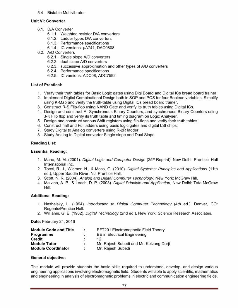
77
5.4 Bistable Multivibrator
Unit VI: Converter
6.1. D/A Converter 6.1.1. Weighted resistor D/A converters 6.1.2. Ladder types D/A converters 6.1.3. Performance specifications 6.1.4. IC versions: μA741, DAC0808
6.2. A/D Converters 6.2.1. Single slope A/D converters 6.2.2. dual-slope A/D converters 6.2.3. successive approximation and other types of A/D converters 6.2.4. Performance specifications 6.2.5. IC versions: ADC08, ADC7592
List of Practical:
1. Verify their truth tables for Basic Logic gates using Digi Board and Digital ICs bread board trainer. 2. Implement Digital Combinational Design both in SOP and POS for four Boolean variables. Simplify
using K-Map and verify the truth-table using Digital ICs bread board trainer. 3. Construct R-S Flip-flop using NAND Gate and verify its truth tables using Digital ICs. 4. Design and construct A- Synchronous Binary Counters, and synchronous Binary Counters using
J-K Flip flop and verify its truth table and timing diagram on Logic Analyser. 5. Design and construct various Shift registers using flip-flops and verify their truth tables. 6. Construct half and Full adders using basic logic gates and digital LSI chips. 7. Study Digital to Analog converters using R-2R ladder. 8. Study Analog to Digital converter Single slope and Dual Slope.
Reading List:
Essential Reading:
1. Mano, M. M. (2001). Digital Logic and Computer Design (25th Reprint), New Delhi: Prentice–Hall International Inc.
2. Tocci, R. J., Widmer, N., & Moss, G. (2010). Digital Systems: Principles and Applications (11th ed.), Upper Saddle River, NJ: Prentice Hall.
3. Scott, N. R. (2004). Analog and Digital Computer Technology, New York: McGraw Hill. 4. Malvino, A. P., & Leach, D. P. (2003). Digital Principle and Application, New Delhi: Tata McGraw
Hill.
Additional Reading:
1. Nashelsky, L. (1994). Introduction to Digital Computer Technology (4th ed.), Denver, CO: Regents/Prentice Hall.
2. Williams, G. E. (1982). Digital Technology (2nd ed.), New York: Science Research Associates.
Date: February 24, 2016
Module Code and Title : EFT201 Electromagnetic Field Theory Programme : BE in Electrical Engineering Credit : 12 Module Tutor : Mr. Rajesh Subedi and Mr. Kelzang Dorji Module Coordinator : Mr. Rajesh Subedi General objective: This module will provide students the basic skills required to understand, develop, and design various engineering applications involving electromagnetic field. Students will able to apply scientific, mathematics and engineering in analysis of electromagnetic problems in electric and communication engineering fields.
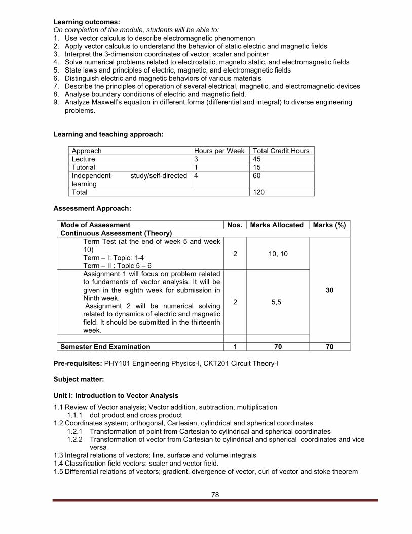
78
Learning outcomes: On completion of the module, students will be able to: 1. Use vector calculus to describe electromagnetic phenomenon 2. Apply vector calculus to understand the behavior of static electric and magnetic fields 3. Interpret the 3-dimension coordinates of vector, scaler and pointer 4. Solve numerical problems related to electrostatic, magneto static, and electromagnetic fields 5. State laws and principles of electric, magnetic, and electromagnetic fields 6. Distinguish electric and magnetic behaviors of various materials 7. Describe the principles of operation of several electrical, magnetic, and electromagnetic devices 8. Analyse boundary conditions of electric and magnetic field. 9. Analyze Maxwell’s equation in different forms (differential and integral) to diverse engineering
problems.
Learning and teaching approach:
Approach Hours per Week Total Credit Hours Lecture 3 45 Tutorial 1 15 Independent study/self-directed learning
4 60
Total 120 Assessment Approach:
Mode of Assessment Nos. Marks Allocated Marks (%) Continuous Assessment (Theory)
Term Test (at the end of week 5 and week 10) Term – I: Topic: 1-4 Term – II : Topic 5 – 6
2 10, 10
30
Assignment 1 will focus on problem related to fundaments of vector analysis. It will be given in the eighth week for submission in Ninth week. Assignment 2 will be numerical solving related to dynamics of electric and magnetic field. It should be submitted in the thirteenth week.
2 5,5
Semester End Examination 1 70 70
Pre-requisites: PHY101 Engineering Physics-I, CKT201 Circuit Theory-I Subject matter: Unit I: Introduction to Vector Analysis
1.1 Review of Vector analysis; Vector addition, subtraction, multiplication 1.1.1 dot product and cross product
1.2 Coordinates system; orthogonal, Cartesian, cylindrical and spherical coordinates 1.2.1 Transformation of point from Cartesian to cylindrical and spherical coordinates 1.2.2 Transformation of vector from Cartesian to cylindrical and spherical coordinates and vice
versa 1.3 Integral relations of vectors; line, surface and volume integrals 1.4 Classification field vectors: scaler and vector field. 1.5 Differential relations of vectors; gradient, divergence of vector, curl of vector and stoke theorem
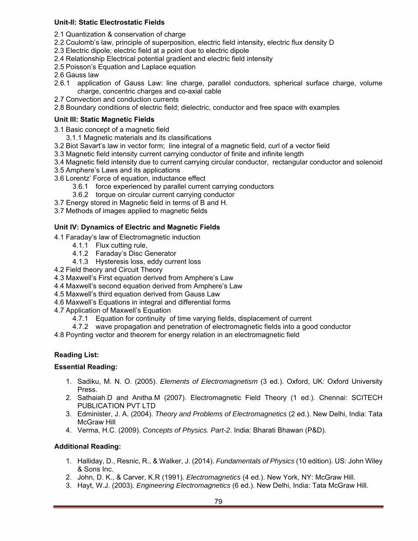
79
Unit-II: Static Electrostatic Fields
2.1 Quantization & conservation of charge 2.2 Coulomb’s law, principle of superposition, electric field intensity, electric flux density D 2.3 Electric dipole; electric field at a point due to electric dipole 2.4 Relationship Electrical potential gradient and electric field intensity 2.5 Poisson’s Equation and Laplace equation 2.6 Gauss law 2.6.1 application of Gauss Law: line charge, parallel conductors, spherical surface charge, volume
charge, concentric charges and co-axial cable 2.7 Convection and conduction currents 2.8 Boundary conditions of electric field; dielectric, conductor and free space with examples
Unit III: Static Magnetic Fields
3.1 Basic concept of a magnetic field 3.1.1 Magnetic materials and its classifications 3.2 Biot Savart’s law in vector form; line integral of a magnetic field, curl of a vector field 3.3 Magnetic field intensity current carrying conductor of finite and infinite length 3.4 Magnetic field intensity due to current carrying circular conductor, rectangular conductor and solenoid 3.5 Amphere’s Laws and its applications 3.6 Lorentz’ Force of equation, inductance effect
3.6.1 force experienced by parallel current carrying conductors 3.6.2 torque on circular current carrying conductor
3.7 Energy stored in Magnetic field in terms of B and H. 3.7 Methods of images applied to magnetic fields
Unit IV: Dynamics of Electric and Magnetic Fields
4.1 Faraday’s law of Electromagnetic induction 4.1.1 Flux cutting rule, 4.1.2 Faraday’s Disc Generator 4.1.3 Hysteresis loss, eddy current loss
4.2 Field theory and Circuit Theory 4.3 Maxwell’s First equation derived from Amphere’s Law 4.4 Maxwell’s second equation derived from Amphere’s Law 4.5 Maxwell’s third equation derived from Gauss Law 4.6 Maxwell’s Equations in integral and differential forms 4.7 Application of Maxwell’s Equation
4.7.1 Equation for continuity of time varying fields, displacement of current 4.7.2 wave propagation and penetration of electromagnetic fields into a good conductor
4.8 Poynting vector and theorem for energy relation in an electromagnetic field
Reading List:
Essential Reading:
1. Sadiku, M. N. O. (2005). Elements of Electromagnetism (3 ed.). Oxford, UK: Oxford University Press.
2. Sathaiah.D and Anitha.M (2007). Electromagnetic Field Theory (1 ed.). Chennai: SCITECH PUBLICATION PVT LTD
3. Edminister, J. A. (2004). Theory and Problems of Electromagnetics (2 ed.). New Delhi, India: Tata McGraw Hill
4. Verma, H.C. (2009). Concepts of Physics. Part-2. India: Bharati Bhawan (P&D).
Additional Reading:
1. Halliday, D., Resnic, R., & Walker, J. (2014). Fundamentals of Physics (10 edition). US: John Wiley & Sons Inc.
2. John, D. K., & Carver, K.R (1991). Electromagnetics (4 ed.). New York, NY: McGraw Hill. 3. Hayt, W.J. (2003). Engineering Electromagnetics (6 ed.). New Delhi, India: Tata McGraw Hill.
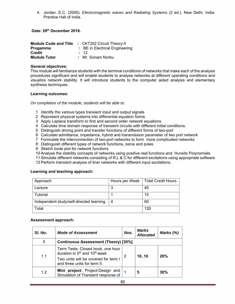
80
4. Jordan, E.C. (2005). Electromagnetic waves and Radiating Systems (2 ed.). New Delhi, India: Prentice Hall of India.
Date: 29th December 2016.
Module Code and Title : CKT202 Circuit Theory-II Progamme : BE in Electrical Engineering Credit : 12 Module Tutor : Mr. Sonam Norbu General objectives: This module will familiarize students with the terminal conditions of networks that make each of the analysis procedures significant and will enable students to analyse networks at different operating conditions and visualize network stability. It will introduce students to the computer aided analysis and elementary synthesis techniques. Learning outcomes: On completion of the module, students will be able to:
1 Identify the various types transient input and output signals 2 Represent physical systems into differential equation forms. 3 Apply Laplace transform to first and second order network equations. 4 Calculate time domain response of transient circuits with different initial conditions. 5 Distinguish driving point and transfer functions of different forms of two-port 6 Calculate admittance, impedance, hybrid and transmission parameter of two port network 7 Formulate the interconnection of two-port networks to form more complicated networks 8 Distinguish different types of network functions, zeros and poles 9 Sketch bode plot for network functions 10 Analyse the stability concepts of networks using positive real functions and Hurwitz Polynomials 11 Simulate different networks consisting of R,L & C for different excitations using appropriate software 12 Perform transient analysis of liner networks with different input excitations.
Learning and teaching approach:
Approach Hours per Week Total Credit Hours
Lecture 3 45
Tutorial 1 15
Independent study/self-directed learning 4 60
Total 120
Assessment approach:
Sl. No. Mode of Assessment Nos. Marks Allocated
Marks (%)
1 Continuous Assessment (Theory) [30%]
1.1
Term Tests: Closed book, one hour duration in 5th and 10th week
Two units will be covered for term I and three units for term II.
2 10, 10 20%
1.2 Mini project: Project-Design and Simulation of Transient response of
1 5 30%
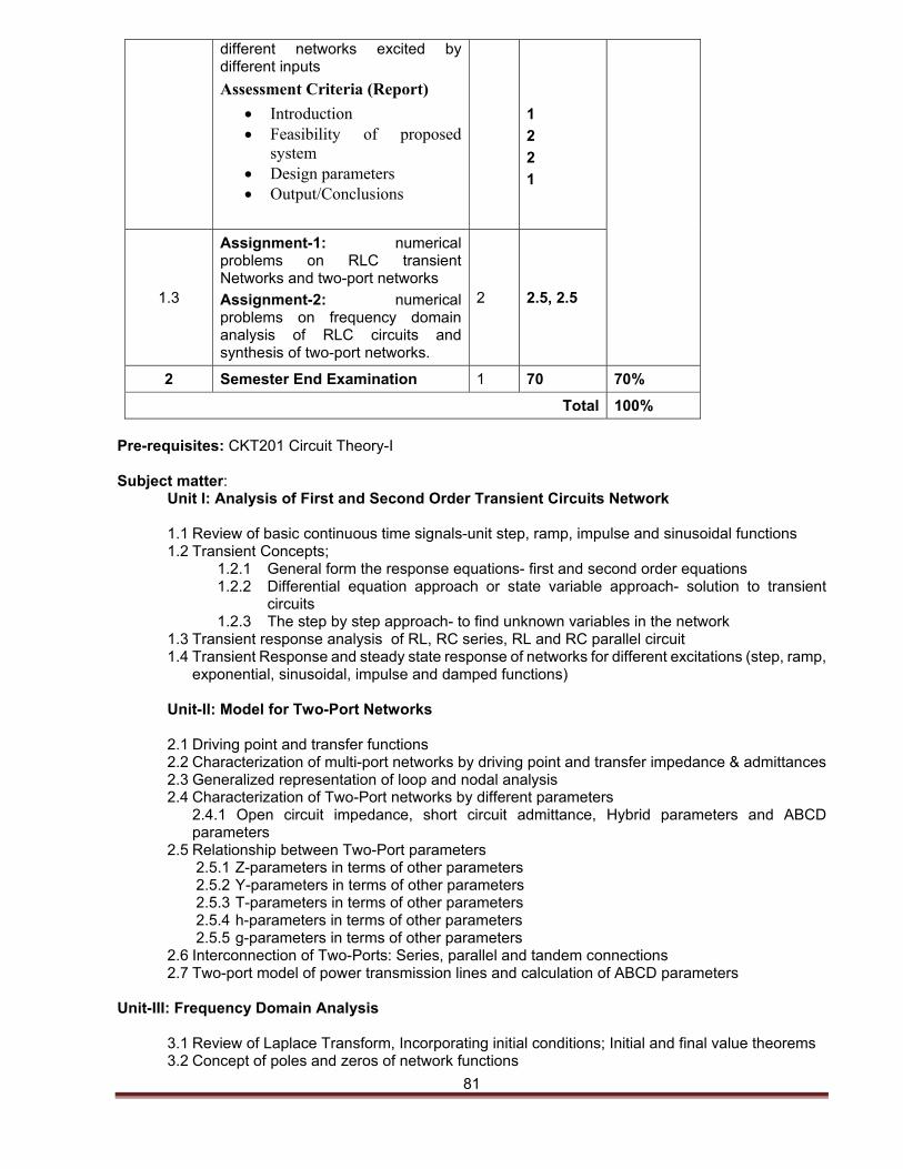
81
different networks excited by different inputs
Assessment Criteria (Report)
Introduction Feasibility of proposed
system Design parameters Output/Conclusions
1
2
2
1
1.3
Assignment-1: numerical problems on RLC transient Networks and two-port networks
Assignment-2: numerical problems on frequency domain analysis of RLC circuits and synthesis of two-port networks.
2 2.5, 2.5
2 Semester End Examination 1 70 70%
Total 100%
Pre-requisites: CKT201 Circuit Theory-I Subject matter:
Unit I: Analysis of First and Second Order Transient Circuits Network 1.1 Review of basic continuous time signals-unit step, ramp, impulse and sinusoidal functions 1.2 Transient Concepts;
1.2.1 General form the response equations- first and second order equations 1.2.2 Differential equation approach or state variable approach- solution to transient
circuits 1.2.3 The step by step approach- to find unknown variables in the network
1.3 Transient response analysis of RL, RC series, RL and RC parallel circuit 1.4 Transient Response and steady state response of networks for different excitations (step, ramp,
exponential, sinusoidal, impulse and damped functions) Unit-II: Model for Two-Port Networks 2.1 Driving point and transfer functions 2.2 Characterization of multi-port networks by driving point and transfer impedance & admittances 2.3 Generalized representation of loop and nodal analysis 2.4 Characterization of Two-Port networks by different parameters
2.4.1 Open circuit impedance, short circuit admittance, Hybrid parameters and ABCD parameters
2.5 Relationship between Two-Port parameters 2.5.1 Z-parameters in terms of other parameters 2.5.2 Y-parameters in terms of other parameters 2.5.3 T-parameters in terms of other parameters 2.5.4 h-parameters in terms of other parameters 2.5.5 g-parameters in terms of other parameters
2.6 Interconnection of Two-Ports: Series, parallel and tandem connections 2.7 Two-port model of power transmission lines and calculation of ABCD parameters
Unit-III: Frequency Domain Analysis
3.1 Review of Laplace Transform, Incorporating initial conditions; Initial and final value theorems 3.2 Concept of poles and zeros of network functions
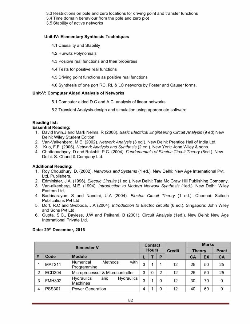
82
3.3 Restrictions on pole and zero locations for driving point and transfer functions 3.4 Time domain behaviour from the pole and zero plot 3.5 Stability of active networks
Unit-IV: Elementary Synthesis Techniques
4.1 Causality and Stability
4.2 Hurwitz Polynomials
4.3 Positive real functions and their properties
4.4 Tests for positive real functions
4.5 Driving point functions as positive real functions
4.6 Synthesis of one port RC, RL & LC networks by Foster and Causer forms.
Unit-V: Computer Aided Analysis of Networks
5.1 Computer aided D.C and A.C. analysis of linear networks
5.2 Transient Analysis-design and simulation using appropriate software
Reading list: Essential Reading:
1. David Irwin.J and Mark Nelms. R (2008). Basic Electrical Engineering Circuit Analysis (9 ed).New Delhi: Wiley Student Edition.
2. Van-Valkenberg, M.E. (2002). Network Analysis (3 ed.). New Delhi: Prentice Hall of India Ltd. 3. Kuo, F.F. (2005). Network Analysis and Synthesis (2 ed.). New York: John Wiley & sons. 4. Chattopadhyay, D and Rakshit, P.C. (2004). Fundamentals of Electric Circuit Theory (6ed.). New
Delhi: S. Chand & Company Ltd. Additional Reading:
1. Roy Choudhury, D. (2002). Networks and Systems (1 ed.). New Delhi: New Age International Pvt. Ltd. Publishers.
2. Edminister, J.A. (1996). Electric Circuits (1 ed.). New Delhi: Tata Mc Graw Hill Publishing Company. 3. Van-alkenberg, M.E. (1994). Introduction to Modern Network Synthesis (1ed.). New Delhi: Wiley
Eastern Ltd. 4. Badrinarayan, S and Nandini, U.A (2004). Electric Circuit Theory (1 ed.). Chennai: Scitech
Publications Pvt Ltd. 5. Dorf, R.C and Svoboda, J.A (2004). Introduction to Electric circuits (6 ed.). Singapore: John Wiley
and Sons Pvt Ltd. 6. Gupta, S.C., Bayless, J.W and Peikanri, B (2001). Circuit Analysis (1ed.). New Delhi: New Age
International Private Ltd.
Date: 29th December, 2016
Semester V Contact Hours Credit
Marks
Theory Pract# Code Module L T P CA EX CA
1 MAT311 Numerical Methods with Programming
3 1 1 12 25 50 25
2 ECD304 Microprocessor & Microcontroller 3 0 2 12 25 50 25
3 FMH302 Hydraulics and Hydraulics Machines
3 1 0 12 30 70 0
4 PSS301 Power Generation 4 1 0 12 40 60 0
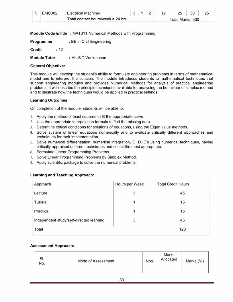
83
5 EMC302 Electrical Machine-II 3 1 2 12 25 50 25
Total contact hours/week = 24 hrs Total Marks=500 Module Code &Title : MAT311 Numerical Methods with Programming
Programme : BE in Civil Engineering
Credit : 12
Module Tutor : Mr. S.T.Venkatesan
General Objective:
This module will develop the student’s ability to formulate engineering problems in terms of mathematical model and to interpret the solution. The module introduces students to mathematical techniques that support engineering modules and provides Numerical Methods for analysis of practical engineering problems. It will describe the principle techniques available for analysing the behaviour of simplex method and to illustrate how the techniques would be applied in practical settings.
Learning Outcomes:
On completion of the module, students will be able to:
1. Apply the method of least squares to fit the appropriate curve. 2. Use the appropriate interpolation formula to find the missing data. 3. Determine critical conditions for solutions of equations, using the Eigen value methods. 4. Solve system of linear equations numerically and to evaluate critically different approaches and
techniques for their implementation. 5. Solve numerical differentiation, numerical integration, O. D. E’s using numerical techniques, having
critically appraised different techniques and select the most appropriate. 6. Formulate Linear Programming Problems 7. Solve Linear Programming Problems by Simplex Method. 8. Apply scientific package to solve the numerical problems.
Learning and Teaching Approach:
Approach Hours per Week Total Credit Hours
Lecture 3 45
Tutorial 1 15
Practical 1 15
Independent study/self-directed learning 3 45
Total 120
Assessment Approach:
Sl. No.
Mode of Assessment Nos.
Marks Allocated
Marks (%)
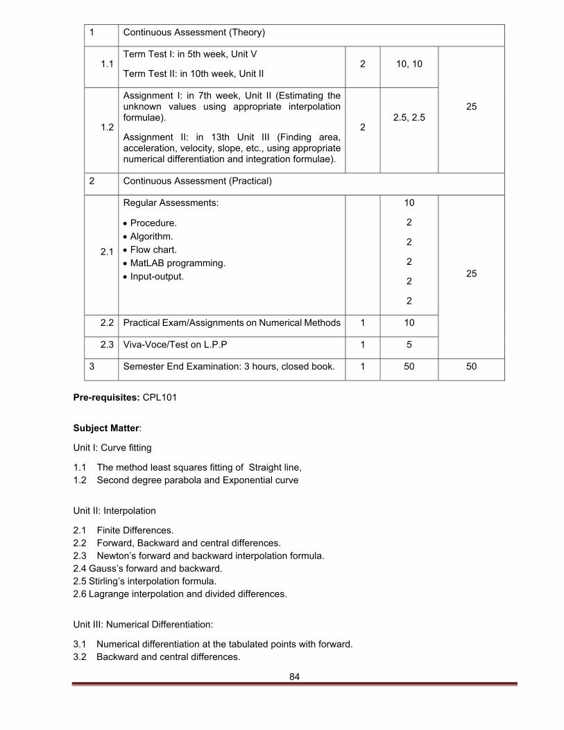
84
1 Continuous Assessment (Theory)
1.1 Term Test I: in 5th week, Unit V
Term Test II: in 10th week, Unit II 2 10, 10
25
1.2
Assignment I: in 7th week, Unit II (Estimating the unknown values using appropriate interpolation formulae).
Assignment II: in 13th Unit III (Finding area, acceleration, velocity, slope, etc., using appropriate numerical differentiation and integration formulae).
2 2.5, 2.5
2 Continuous Assessment (Practical)
2.1
Regular Assessments:
Procedure.
Algorithm.
Flow chart.
MatLAB programming.
Input-output.
10
2
2
2
2
2
25
2.2 Practical Exam/Assignments on Numerical Methods 1 10
2.3 Viva-Voce/Test on L.P.P 1 5
3 Semester End Examination: 3 hours, closed book. 1 50 50
Pre-requisites: CPL101
Subject Matter:
Unit I: Curve fitting
1.1 The method least squares fitting of Straight line, 1.2 Second degree parabola and Exponential curve
Unit II: Interpolation
2.1 Finite Differences. 2.2 Forward, Backward and central differences. 2.3 Newton’s forward and backward interpolation formula. 2.4 Gauss’s forward and backward. 2.5 Stirling’s interpolation formula. 2.6 Lagrange interpolation and divided differences.
Unit III: Numerical Differentiation:
3.1 Numerical differentiation at the tabulated points with forward. 3.2 Backward and central differences.
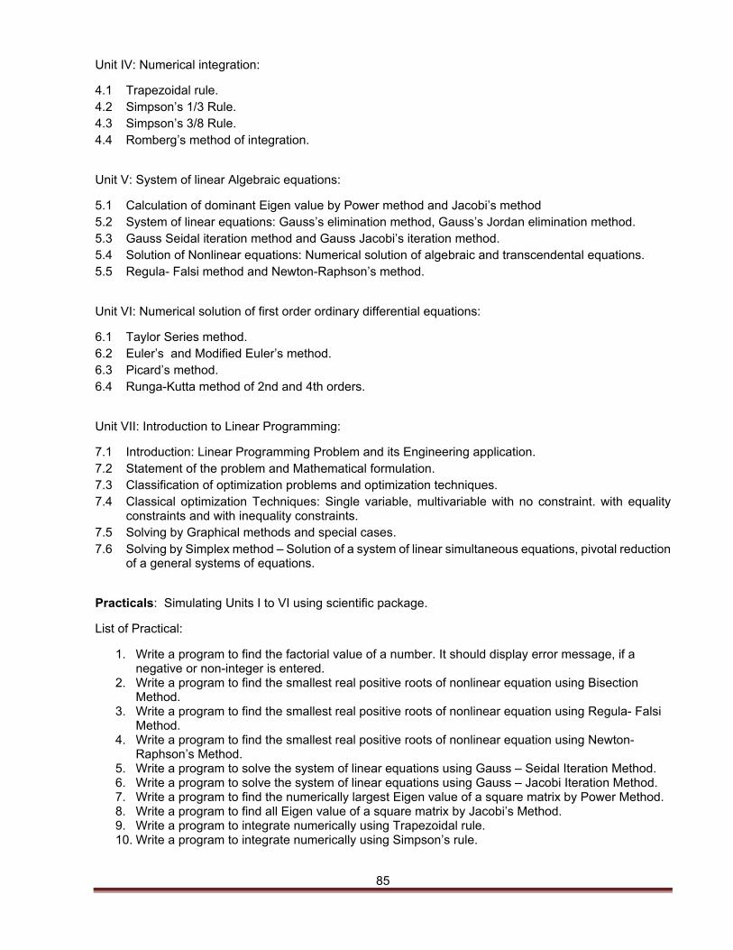
85
Unit IV: Numerical integration:
4.1 Trapezoidal rule. 4.2 Simpson’s 1/3 Rule. 4.3 Simpson’s 3/8 Rule. 4.4 Romberg’s method of integration.
Unit V: System of linear Algebraic equations:
5.1 Calculation of dominant Eigen value by Power method and Jacobi’s method 5.2 System of linear equations: Gauss’s elimination method, Gauss’s Jordan elimination method. 5.3 Gauss Seidal iteration method and Gauss Jacobi’s iteration method. 5.4 Solution of Nonlinear equations: Numerical solution of algebraic and transcendental equations. 5.5 Regula- Falsi method and Newton-Raphson’s method.
Unit VI: Numerical solution of first order ordinary differential equations:
6.1 Taylor Series method. 6.2 Euler’s and Modified Euler’s method. 6.3 Picard’s method. 6.4 Runga-Kutta method of 2nd and 4th orders.
Unit VII: Introduction to Linear Programming:
7.1 Introduction: Linear Programming Problem and its Engineering application. 7.2 Statement of the problem and Mathematical formulation. 7.3 Classification of optimization problems and optimization techniques. 7.4 Classical optimization Techniques: Single variable, multivariable with no constraint. with equality
constraints and with inequality constraints. 7.5 Solving by Graphical methods and special cases. 7.6 Solving by Simplex method – Solution of a system of linear simultaneous equations, pivotal reduction
of a general systems of equations.
Practicals: Simulating Units I to VI using scientific package.
List of Practical:
1. Write a program to find the factorial value of a number. It should display error message, if a negative or non-integer is entered.
2. Write a program to find the smallest real positive roots of nonlinear equation using Bisection Method.
3. Write a program to find the smallest real positive roots of nonlinear equation using Regula- Falsi Method.
4. Write a program to find the smallest real positive roots of nonlinear equation using Newton-Raphson’s Method.
5. Write a program to solve the system of linear equations using Gauss – Seidal Iteration Method. 6. Write a program to solve the system of linear equations using Gauss – Jacobi Iteration Method. 7. Write a program to find the numerically largest Eigen value of a square matrix by Power Method. 8. Write a program to find all Eigen value of a square matrix by Jacobi’s Method. 9. Write a program to integrate numerically using Trapezoidal rule. 10. Write a program to integrate numerically using Simpson’s rule.
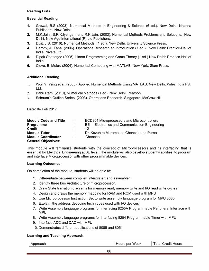
86
Reading Lists:
Essential Reading
1. Grewal, B.S (2003). Numerical Methods in Engineering & Science (6 ed.). New Delhi: Khanna Publishers, New Delhi.
2. M.K.Jain., S.R.K.Iyengar., and R.K.Jain. (2002). Numerical Methods Problems and Solutions. New Delhi: New Age International (P) Ltd Publishers.
3. Dixit, J.B. (2016). Numerical Methods ( 1 ed.). New Delhi. University Science Press. 4. Hamdy, A. Taha. (2006). Operations Research an Introduction (7 ed.). New Delhi: Prentice-Hall of
India Private Ltd. 5. Dipak Chatterjee (2005). Linear Programming and Game Theory (1 ed.).New Delhi: Prentice-Hall of
India. 6. Cleve, B. Moler. (2004). Numerical Computing with MATLAB. New York: Siam Press.
Additional Reading
1. Won Y. Yang et al. (2005). Applied Numerical Methods Using MATLAB. New Delhi: Wiley India Pvt. Ltd.
2. Babu Ram. (2010), Numerical Methods (1 ed). New Delhi: Pearson. 3. Schaum’s Outline Series. (2003). Operations Research. Singapore: McGraw Hill.
Date: 04 Feb 2017
Module Code and Title : ECD304 Microprocessors and Microcontrollers Programme : BE in Electronics and Communication Engineering Credit : 12 Module Tutor : Dr. Kazuhiro Muramatsu, Chencho and Purna Module Coordinator : Chencho General Objectives:
This module will familiarize students with the concept of Microprocessors and its interfacing that is essential for Electrical Engineering at BE level. The module will also develop student’s abilities, to program and interface Microprocessor with other programmable devices.
Learning Outcomes:
On completion of the module, students will be able to:
1. Differentiate between compiler, interpreter, and assembler
2. Identify three bus Architecture of microprocessor.
3. Draw State transition diagrams for memory read, memory write and I/O read write cycles
4. Design and draws the memory mapping for RAM and ROM used with MPU
5. Use Microprocessor Instruction Set to write assembly language program for MPU 8085
6. Explain the address decoding techniques used with I/O devices
7. Write Assembly language programs for interfacing 8255A Programmable Peripheral Interface with MPU.
8. Write Assembly language programs for interfacing 8254 Programmable Timer with MPU
9. Interface ADC and DAC with MPU
10. Demonstrates different applications of 8085 and 8051
Learning and Teaching Approach:
Approach Hours per Week Total Credit Hours
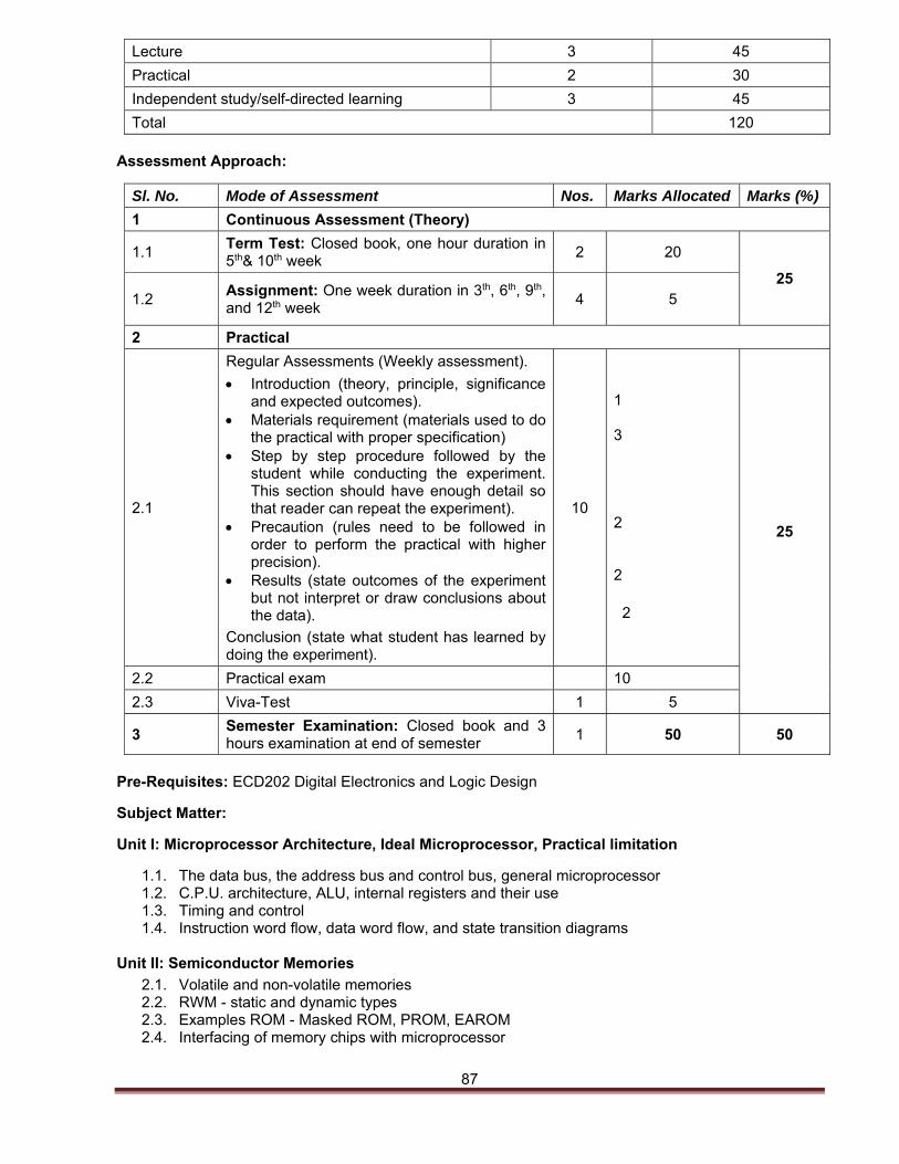
87
Lecture 3 45
Practical 2 30
Independent study/self-directed learning 3 45
Total 120 Assessment Approach:
Sl. No. Mode of Assessment Nos. Marks Allocated Marks (%)
1 Continuous Assessment (Theory)
1.1 Term Test: Closed book, one hour duration in 5th& 10th week
2 20
25 1.2
Assignment: One week duration in 3th, 6th, 9th, and 12th week
4 5
2 Practical
2.1
Regular Assessments (Weekly assessment).
Introduction (theory, principle, significance and expected outcomes).
Materials requirement (materials used to do the practical with proper specification)
Step by step procedure followed by the student while conducting the experiment. This section should have enough detail so that reader can repeat the experiment).
Precaution (rules need to be followed in order to perform the practical with higher precision).
Results (state outcomes of the experiment but not interpret or draw conclusions about the data).
Conclusion (state what student has learned by doing the experiment).
10
1
3
2
2 2
25
2.2 Practical exam 10
2.3 Viva-Test 1 5
3 Semester Examination: Closed book and 3 hours examination at end of semester
1 50 50
Pre-Requisites: ECD202 Digital Electronics and Logic Design
Subject Matter:
Unit I: Microprocessor Architecture, Ideal Microprocessor, Practical limitation
1.1. The data bus, the address bus and control bus, general microprocessor 1.2. C.P.U. architecture, ALU, internal registers and their use 1.3. Timing and control 1.4. Instruction word flow, data word flow, and state transition diagrams
Unit II: Semiconductor Memories
2.1. Volatile and non-volatile memories 2.2. RWM - static and dynamic types 2.3. Examples ROM - Masked ROM, PROM, EAROM 2.4. Interfacing of memory chips with microprocessor
88
Unit III: Microprocessor Instruction Set (8085/8086)
3.1. Addressing modes, status register with C, Z, S, P, and AC flags 3.2. The binary code, hexadecimal code for each instruction 3.3. Opcode fetch machine cycle 3.4. WRITE / READ machine cycle 3.5. Interrupt acknowledge machine cycle and their Timing diagrams, Memory mapping 3.6. Address decoding technique, memory mapped I/O and peripheral mapped I/O) Interrupts, RST
and hardware interrupts 3.7. Brief idea of assembler, compiler, loader, monitor and other software aids, software development
methodology 3.8. Assembly language fundamentals and programming 3.9. M.L. programming, simple examples with subroutines
Unit IV: 8255A Programmable Peripheral Interface
4.1. Pin configuration
4.2. Logic symbolism functional description 4.3. Operating modes, interfacing and programming of the device 4.4. Introduction to 8237 (DMA handler) and 8259 (Interrupt handler)
Unit V: 8254 Programmable Timer
5.1. Pin configuration 5.2. Logic symbolism and Functional description 5.3. Interfacing 5.4. Operating modes and Programming of the device
Unit VI: ADC and DAC
6.1. ADC 0800 I.C Chips
6.2. Their pin configurations 6.3. Logic symbolisms 6.4. Functional description 6.5. Sample and hold 6.6. Interfacing and subroutines
Unit VII: INTEL 8051 Microcontroller
7.1. Architecture of 8051
7.2. Memory organisation 7.3. Addressing modes 7.4. Instruction set 7.5. Boolean processing 7.6. Simple programs
Unit VIII: Microprocessor and Microcontroller Applications
8.1. Microprocessor and microcontroller selection 8.2. Design methodology 8.3. Simple examples of applications 8.4. Numerical relays
List of Practical:
1. Basic introduction to assembly instructions. (Free rudimental assembly software for PC is available online.)
2. Introduction to 8085/8086 Microprocessor Kit – memory mapping for the assigned kit, utility programs
3. Assembly language problems – to verify and observe the output of assembly program using basic data transfer and data manipulation method
4. To write language program stowing looping, counting and indexing
89
5. To study the Stack and Subroutines 6. BCD Arithmetic and Code Conversion 7. Interfacing of DAC to Microprocessor 8086 8. Interfacing of ADC to Microprocessor 8086 9. Interfacing Seven segment LED displays 10. Serial transmission & Interrupt handling
Reading List:
Essential Reading:
1. Gaonkar, R. S. (2013). Microprocessor Architecture, Programming and Applications with the 8085 (6 ed.). Mumbai, India: Penram International Publishing.
2. Rifiquazzaman, M. (1987). Microcomputer Theory and Application with the Intel SDK-85 (2 ed.). New York, NY: John Willey & Sons.
3. Barry B. Brey (2013), The Intel Microprocessors: Pearson New International Edition (8 ed.). London, UK: Pearson.
Additional Reading:
1. Srinath, N. K. (2005). 8085 Microprocessor: Programming and Interfacing (2 ed.). New Delhi, India: PHI Learning.
2. Short, K. L. (2003). Microprocessors and Programme Logic (2 ed.). London, UK: Pearson. 3. Mathur, A.P (2001). Introduction to Microprocessors (3 ed.). New Delhi, India: McGraw Hill
Education India Private Ltd. 4. Liu, Y.-C., & Gibson, G. A. (2005). Microcomputer Systems: The 8086/8088 Family Architecture
Programming and Design (2 ed.). London, UK: Pearson. 5. Leventhal, L. A. (1978). 8080A/8085 Assembly Language Programming. New York, NY: McGraw
Hill. 6. Tokheim, R. L. (1986). Schaum's Outline of Theory and Problems of Microprocessor Fundamentals
(2 ed.). New York, NY: McGraw Hill. 7. Pal, A. (1989). Microprocessors: Principles and Applications. New York, NY: McGraw Hill. 8. Pal, A. (2011). Microcontrollers: Principles and Applications. New Delhi, India: PHI Learning.
Date: February 24, 2016
Module Code and Title : FMH302 Hydraulics and Hydraulic Machines Program : BE Electrical Engineering Credit : 12 Module Tutor : Mr. Om Kafley General objectives: This module introduces electrical engineering students to the fundamental of fluid mechanics. The working principle and different efficiencies of impulse and reaction turbines will be discussed. Students will learn the working of principle of a centrifugal pump. Students will find the knowledge of mathematics very useful in the analysis of fluid mechanics problems. Learning outcomes: On completion of the module, students will be able to:
1. compute the properties of fluid. 2. Calculate pressure acting at a point and explain the various method of measuring pressure. 3. Calculate the forces that act on submerged planes and curves. 4. Apply Bernoulli’s equation to real fluid motions 5. Draw hydraulic and energy grade lines. 6. Calculate power transmitted through pipes. 7. Identify the main features of a hydroelectric power plant. 8. Classify various turbines; Pelton, Francis and Kaplan turbines
90
9. Explain the volumetric efficiency, hydraulic efficiency, mechanical efficiency and plant efficiency. 10. Explain the constructional details and the working principles of Centrifugal pumps.
Learning and teaching approach: Mostly by lecture, but students are expected to support the module by reading from some of the suggested texts. The particular texts normally chosen to be appropriate to students own interest and background study. Lectures introduce concepts and provide a broad background; demonstrations are used to clarify particular points of detail or to illustrate concepts. Tests and worksheets are used to help students to monitor their own progress through the module. Approach Hours per week Total Credit Hours Lecture 3 45 Tutorial 1 15 Self - study 4 60 Total 120
Assessment Approach:
Mode of Assessment Nos. Marks Allocated Marks (%) Continuous Assessment (Theory)
Term Test (at the end of week 5 and week 10) Term – I: Topic: 1-4 Term – II : Topic 5 – 6
2 10 X 2 = 20
30
Assignment 1 will focus on problem related to fundaments of fluid mechanics. It will be given in the eighth week for submission in Ninth week. Assignment 2 will be related to hydraulic machine. It should be submitted in the thirteenth week.
2 5X2 =10
Semester End Examination 1 70 70
Pre-requisites: Engineering Mechanics, Engineering Mathematics - I Subject matter:
1. Properties of fluids: 1.1. Development of fluid mechanics 1.2. Definition and explain fluid-Mass density, Specific weight and Specific gravity 1.3. Explain Viscosity and Newton's law of viscosity 1.4. Explain Compressibility of fluid and its relationship with Bulk modulus. 1.5. Explain Universal gas law 1.6. Explain Vapour pressure, Surface tension and Capillarity.
2. Pressure Measurement: 2.1. Define Pascal’s law 2.2. Explain and shoe the pressure variation with depth of liquid 2.3. Show the relationship between Atmospheric pressure, Absolute,gauge and vacuum pressure 2.4. Explain the method of pressure measurement using different types of manomenters and
mechanical gauges.
3. Hydrostatics: 1.1. Calculate hydrostatic pressure, centre of pressure on submerged bodies on horizontal plane
and vertical plane, inclined plane and curved surfaces. 1.2. Draw pressure diagram
91
4. Fluid kinematics: 4.1. Explain the following types of flow: Laminar and turbulent flow, Uniform and Non-Uniform flow,
Compressible and incompressible flow, Ideal and real fluid, Rotational and Irrotational flow, One-dimensional, Two-dimensional and Three-dimensional flow.
4.2. Explain and derive Continuity Equation for in-compressible flow only
5. Fluid Dynamics: 5.1. Identify the forces acting on fluid in motion, identify the forces considered in Reynold’s equation
of motion, Navier Stroke and Euler’s equations of motion. 5.2. Derive Euler’s equation of motion. 5.3. Derive Bernoulli's equation and explain the datum energy, pressure energy and Potential energy
of fluid flow 5.4. Identify the unit of energy in Bernouli’s equation. State the assumption made in developing the
energy equation. 5.5. Modify Bernoulli’s equation to apply to real fluids. 5.6. Explain momentum equation for fluid flow and calculate the force exerted on bend of a pipe. 6. Flow through pipes: 6.1. Explain major losses and minor losses in pipe flow. 6.2. Derive Darcy-Weisbach formula 6.3. Explain and draw hydraulic gradient and total energy lines. 6.4. Calculate amount of power transmitted through pipes and condition for maximum power
transmission 6.5. Calculate the diameter of nozzle for maximum power transmission 6.6. Explain water hammering phenomena.
7. Impact of Free Jets:
7.1. Calculate the force exerted by fluid jet on stationary flat plate, moving plate, stationary curved vane and moving curved vane.
7.2. Draw velocity triangle at inlet and outlet and differentiate between velocity of flow and velocity of whirl.
7.3. Derive the law of hydraulic machine 8. Hydraulic Turbines:
8.1. Classification of hydraulic turbines 8.2. Explain the constructional details of Pelton wheel, Francis and Kaplan turbines and function of
each part. 8.3. Explain cavitation in reaction turbine. 8.4. Explain and calculate the various types of efficiencies (volumetric, hydraulic, mechanical,
generator, plant efficiency) 9. Centrifugal Pumps:
9.1. Explain the constructional detail and working principle of centrifugal pump. 9.2. Calculate the work done by the impeller-Head, Losses and efficiencies 9.3. Find minimum starting speed 9.4. Explain specific speed 9.5. Explain multi-stage pumps, pumps in parallel, performance of pumps, priming, pumps troubles
and remedies. 9.6. Explain cavitation in pump.
Essential Readings:
1. Modi, P.N. & Seth, S.M. (2002).Hydraulics and Fluid Mechanics (14 ed.) New Delhi: Standard Book House.
2. Jain, A.K. (2004). A text book of Fluid Mechanics (9 ed.). New Delhi: khanna publisher
3. Jagdish, L. (2003). Hydraulics Machines including fluidics (6 ed.). New Delhi: Metropolitan Book Co.
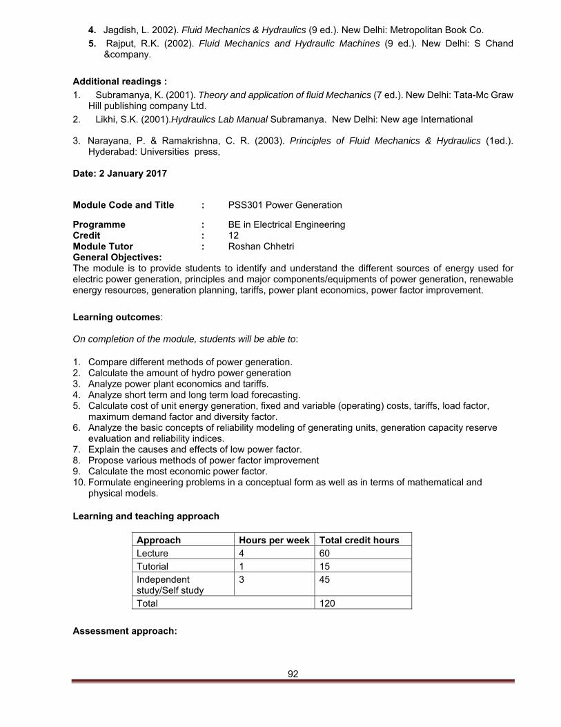
92
4. Jagdish, L. 2002). Fluid Mechanics & Hydraulics (9 ed.). New Delhi: Metropolitan Book Co.
5. Rajput, R.K. (2002). Fluid Mechanics and Hydraulic Machines (9 ed.). New Delhi: S Chand &company.
Additional readings :
1. Subramanya, K. (2001). Theory and application of fluid Mechanics (7 ed.). New Delhi: Tata-Mc Graw Hill publishing company Ltd.
2. Likhi, S.K. (2001).Hydraulics Lab Manual Subramanya. New Delhi: New age International
3. Narayana, P. & Ramakrishna, C. R. (2003). Principles of Fluid Mechanics & Hydraulics (1ed.). Hyderabad: Universities press,
Date: 2 January 2017
Module Code and Title : PSS301 Power Generation
Programme : BE in Electrical Engineering Credit : 12 Module Tutor : Roshan Chhetri General Objectives: The module is to provide students to identify and understand the different sources of energy used for electric power generation, principles and major components/equipments of power generation, renewable energy resources, generation planning, tariffs, power plant economics, power factor improvement.
Learning outcomes: On completion of the module, students will be able to:
1. Compare different methods of power generation. 2. Calculate the amount of hydro power generation 3. Analyze power plant economics and tariffs. 4. Analyze short term and long term load forecasting. 5. Calculate cost of unit energy generation, fixed and variable (operating) costs, tariffs, load factor,
maximum demand factor and diversity factor. 6. Analyze the basic concepts of reliability modeling of generating units, generation capacity reserve
evaluation and reliability indices. 7. Explain the causes and effects of low power factor. 8. Propose various methods of power factor improvement 9. Calculate the most economic power factor. 10. Formulate engineering problems in a conceptual form as well as in terms of mathematical and
physical models.
Learning and teaching approach
Approach Hours per week Total credit hours Lecture 4 60Tutorial 1 15Independent study/Self study
3 45
Total 120
Assessment approach:
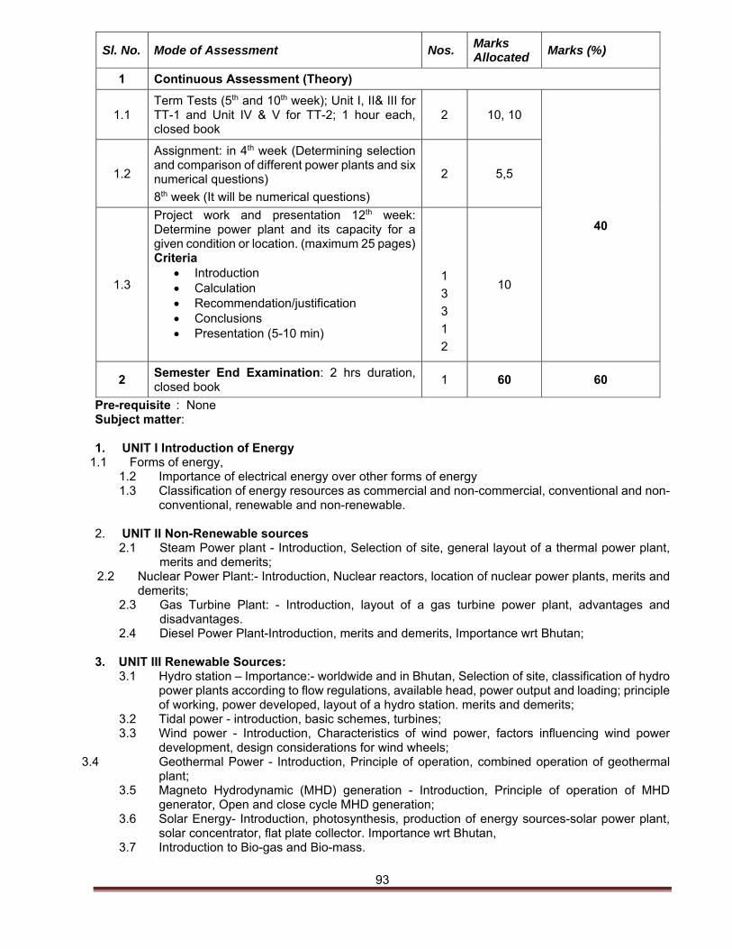
93
Pre-requisite : None Subject matter: 1. UNIT I Introduction of Energy
1.1 Forms of energy, 1.2 Importance of electrical energy over other forms of energy 1.3 Classification of energy resources as commercial and non-commercial, conventional and non-
conventional, renewable and non-renewable. 2. UNIT II Non-Renewable sources
2.1 Steam Power plant - Introduction, Selection of site, general layout of a thermal power plant, merits and demerits;
2.2 Nuclear Power Plant:- Introduction, Nuclear reactors, location of nuclear power plants, merits and demerits;
2.3 Gas Turbine Plant: - Introduction, layout of a gas turbine power plant, advantages and disadvantages.
2.4 Diesel Power Plant-Introduction, merits and demerits, Importance wrt Bhutan; 3. UNIT III Renewable Sources:
3.1 Hydro station – Importance:- worldwide and in Bhutan, Selection of site, classification of hydro power plants according to flow regulations, available head, power output and loading; principle of working, power developed, layout of a hydro station. merits and demerits;
3.2 Tidal power - introduction, basic schemes, turbines; 3.3 Wind power - Introduction, Characteristics of wind power, factors influencing wind power
development, design considerations for wind wheels; 3.4 Geothermal Power - Introduction, Principle of operation, combined operation of geothermal
plant; 3.5 Magneto Hydrodynamic (MHD) generation - Introduction, Principle of operation of MHD
generator, Open and close cycle MHD generation; 3.6 Solar Energy- Introduction, photosynthesis, production of energy sources-solar power plant,
solar concentrator, flat plate collector. Importance wrt Bhutan, 3.7 Introduction to Bio-gas and Bio-mass.
Sl. No. Mode of Assessment Nos. Marks Allocated
Marks (%)
1 Continuous Assessment (Theory)
1.1 Term Tests (5th and 10th week); Unit I, II& III for TT-1 and Unit IV & V for TT-2; 1 hour each, closed book
2 10, 10
40
1.2
Assignment: in 4th week (Determining selection and comparison of different power plants and six numerical questions)
8th week (It will be numerical questions)
2 5,5
1.3
Project work and presentation 12th week: Determine power plant and its capacity for a given condition or location. (maximum 25 pages)Criteria
Introduction Calculation Recommendation/justification Conclusions Presentation (5-10 min)
1
3
3
1
2
10
2 Semester End Examination: 2 hrs duration, closed book
1 60 60
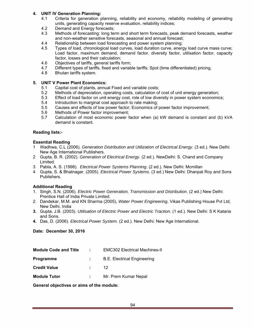
94
4. UNIT IV Generation Planning: 4.1 Criteria for generation planning, reliability and economy, reliability modeling of generating
units, generating capacity reserve evaluation, reliability indices; 4.2 Demand and Energy forecasts; 4.3 Methods of forecasting: long term and short term forecasts, peak demand forecasts, weather
and non-weather sensitive forecasts, seasonal and annual forecast; 4.4 Relationship between load forecasting and power system planning; 4.5 Types of load, chronological load curves, load duration curve, energy load curve mass curve;
Load factor, maximum demand, demand factor, diversity factor, utilisation factor, capacity factor, losses and their calculation;
4.6 Objectives of tariffs, general tariffs form; 4.7 Different types of tariffs, fixed and variable tariffs; Spot (time differentiated) pricing, 4.8 Bhutan tariffs system.
5. UNIT V Power Plant Economics:
5.1 Capital cost of plants, annual Fixed and variable costs; 5.2 Methods of depreciation, operating costs, calculation of cost of unit energy generation; 5.3 Effect of load factor on unit energy cost, role of low diversity in power system economics; 5.4 Introduction to marginal cost approach to rate making; 5.5 Causes and effects of low power factor; Economics of power factor improvement; 5.6 Methods of Power factor improvement; 5.7 Calculation of most economic power factor when (a) kW demand is constant and (b) kVA
demand is constant. Reading lists:- Essential Reading 1 Wadhwa, C.L (2006). Generation Distribution and Utilization of Electrical Energy. (3 ed.). New Delhi:
New Age International Publishers. 2 Gupta, B. R. (2002). Generation of Electrical Energy. (2 ed.). NewDelhi: S. Chand and Company
Limited. 3 Pabla, A. S. (1998). Electrical Power Systems Planning. (2 ed.). New Delhi: Mcmillan 4 Gupta, S. & Bhatnagar. (2005). Electrical Power Systems. (3 ed.) New Delhi: Dhanpat Roy and Sons
Publishers. Additional Reading 1. Singh, S.N. (2006). Electric Power Generation, Transmission and Distribution. (2 ed.) New Delhi:
Prentice Hall of India Private Limited. 2. Dandekar, M.M. and KN Sharma (2005), Water Power Engineering, Vikas Publishing House Pvt Ltd,
New Delhi, India 3. Gupta, J.B. (2003). Utilisation of Electric Power and Electric Traction. (1 ed.). New Delhi: S K Kataria
and Sons. 4. Das, D. (2006). Electrical Power System. (2 ed.). New Delhi: New Age International. Date: December 30, 2016
Module Code and Title : EMC302 Electrical Machines-II
Programme : B.E. Electrical Engineering
Credit Value : 12
Module Tutor : Mr. Prem Kumar Nepal
General objectives or aims of the module:
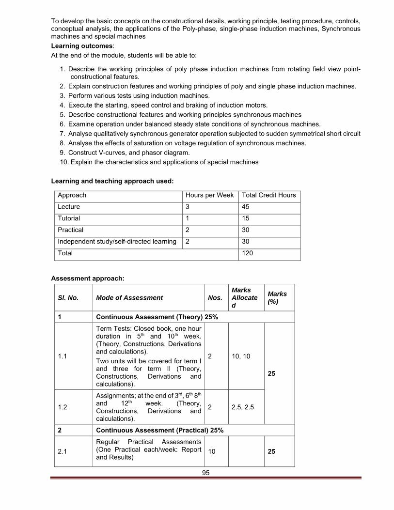
95
To develop the basic concepts on the constructional details, working principle, testing procedure, controls, conceptual analysis, the applications of the Poly-phase, single-phase induction machines, Synchronous machines and special machines
Learning outcomes:
At the end of the module, students will be able to:
1. Describe the working principles of poly phase induction machines from rotating field view point- constructional features.
2. Explain construction features and working principles of poly and single phase induction machines.
3. Perform various tests using induction machines.
4. Execute the starting, speed control and braking of induction motors.
5. Describe constructional features and working principles synchronous machines
6. Examine operation under balanced steady state conditions of synchronous machines.
7. Analyse qualitatively synchronous generator operation subjected to sudden symmetrical short circuit
8. Analyse the effects of saturation on voltage regulation of synchronous machines.
9. Construct V-curves, and phasor diagram.
10. Explain the characteristics and applications of special machines
Learning and teaching approach used:
Approach Hours per Week Total Credit Hours
Lecture 3 45
Tutorial 1 15
Practical 2 30
Independent study/self-directed learning 2 30
Total 120
Assessment approach:
Sl. No. Mode of Assessment Nos. Marks Allocated
Marks (%)
1 Continuous Assessment (Theory) 25%
1.1
Term Tests: Closed book, one hour duration in 5th and 10th week. (Theory, Constructions, Derivations and calculations).
Two units will be covered for term I and three for term II (Theory, Constructions, Derivations and calculations).
2 10, 10
25
1.2
Assignments; at the end of 3rd, 6th 8th and 12th week. (Theory, Constructions, Derivations and calculations).
2 2.5, 2.5
2 Continuous Assessment (Practical) 25%
2.1
Regular Practical Assessments (One Practical each/week: Report and Results)
10
25
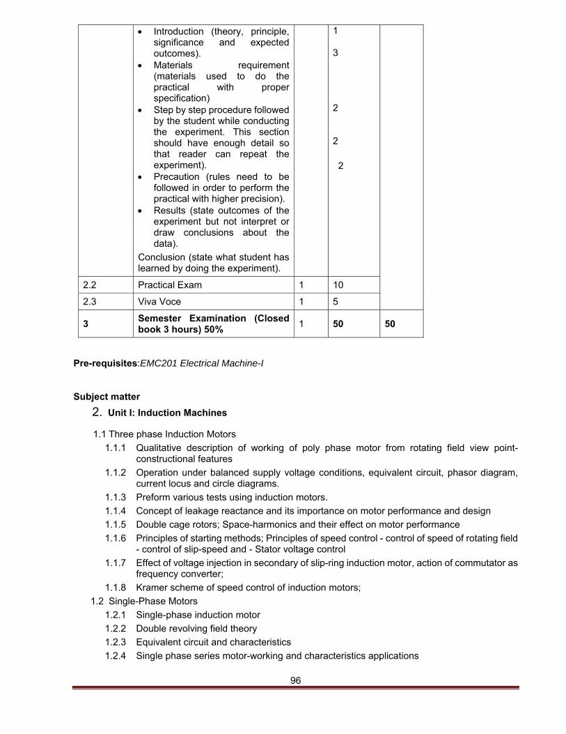
96
Introduction (theory, principle, significance and expected outcomes).
Materials requirement (materials used to do the practical with proper specification)
Step by step procedure followed by the student while conducting the experiment. This section should have enough detail so that reader can repeat the experiment).
Precaution (rules need to be followed in order to perform the practical with higher precision).
Results (state outcomes of the experiment but not interpret or draw conclusions about the data).
Conclusion (state what student has learned by doing the experiment).
1
3
2
2
2
2.2 Practical Exam 1 10
2.3 Viva Voce 1 5
3 Semester Examination (Closed book 3 hours) 50%
1 50 50
Pre-requisites:EMC201 Electrical Machine-I
Subject matter
2. Unit I: Induction Machines
1.1 Three phase Induction Motors
1.1.1 Qualitative description of working of poly phase motor from rotating field view point- constructional features
1.1.2 Operation under balanced supply voltage conditions, equivalent circuit, phasor diagram, current locus and circle diagrams.
1.1.3 Preform various tests using induction motors.
1.1.4 Concept of leakage reactance and its importance on motor performance and design
1.1.5 Double cage rotors; Space-harmonics and their effect on motor performance
1.1.6 Principles of starting methods; Principles of speed control - control of speed of rotating field - control of slip-speed and - Stator voltage control
1.1.7 Effect of voltage injection in secondary of slip-ring induction motor, action of commutator as frequency converter;
1.1.8 Kramer scheme of speed control of induction motors;
1.2 Single-Phase Motors
1.2.1 Single-phase induction motor
1.2.2 Double revolving field theory
1.2.3 Equivalent circuit and characteristics
1.2.4 Single phase series motor-working and characteristics applications
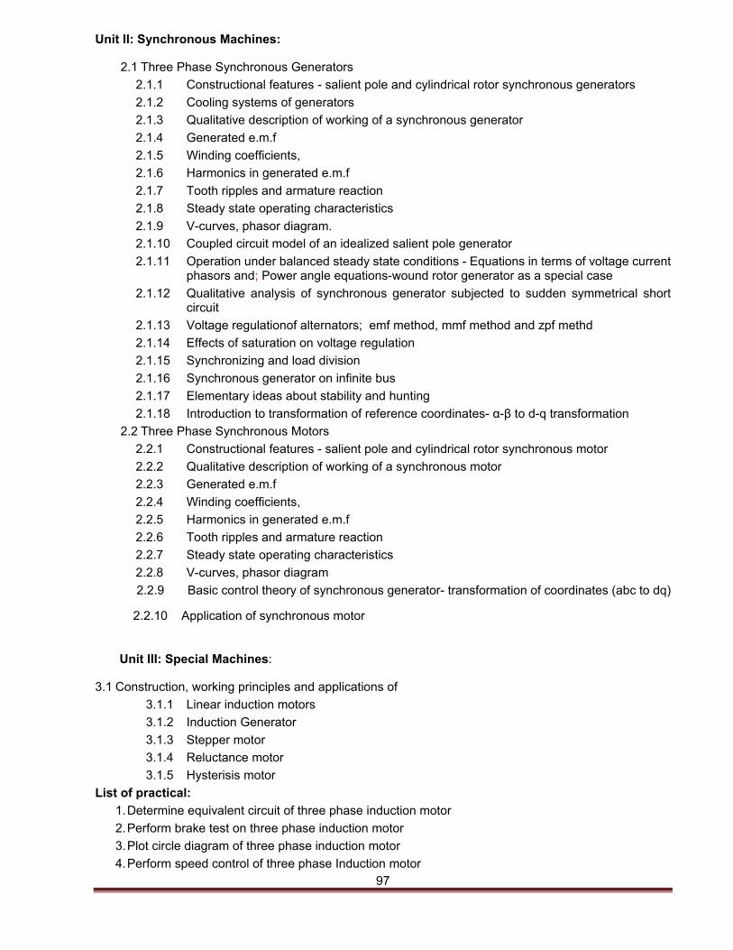
97
Unit II: Synchronous Machines:
2.1 Three Phase Synchronous Generators
2.1.1 Constructional features - salient pole and cylindrical rotor synchronous generators
2.1.2 Cooling systems of generators
2.1.3 Qualitative description of working of a synchronous generator
2.1.4 Generated e.m.f
2.1.5 Winding coefficients,
2.1.6 Harmonics in generated e.m.f
2.1.7 Tooth ripples and armature reaction
2.1.8 Steady state operating characteristics
2.1.9 V-curves, phasor diagram.
2.1.10 Coupled circuit model of an idealized salient pole generator
2.1.11 Operation under balanced steady state conditions - Equations in terms of voltage current phasors and; Power angle equations-wound rotor generator as a special case
2.1.12 Qualitative analysis of synchronous generator subjected to sudden symmetrical short circuit
2.1.13 Voltage regulationof alternators; emf method, mmf method and zpf methd
2.1.14 Effects of saturation on voltage regulation
2.1.15 Synchronizing and load division
2.1.16 Synchronous generator on infinite bus
2.1.17 Elementary ideas about stability and hunting
2.1.18 Introduction to transformation of reference coordinates- α-β to d-q transformation
2.2 Three Phase Synchronous Motors
2.2.1 Constructional features - salient pole and cylindrical rotor synchronous motor
2.2.2 Qualitative description of working of a synchronous motor
2.2.3 Generated e.m.f
2.2.4 Winding coefficients,
2.2.5 Harmonics in generated e.m.f
2.2.6 Tooth ripples and armature reaction
2.2.7 Steady state operating characteristics
2.2.8 V-curves, phasor diagram
2.2.9 Basic control theory of synchronous generator- transformation of coordinates (abc to dq)
2.2.10 Application of synchronous motor
Unit III: Special Machines:
3.1 Construction, working principles and applications of
3.1.1 Linear induction motors
3.1.2 Induction Generator
3.1.3 Stepper motor
3.1.4 Reluctance motor
3.1.5 Hysterisis motor
List of practical:
1. Determine equivalent circuit of three phase induction motor
2. Perform brake test on three phase induction motor
3. Plot circle diagram of three phase induction motor
4. Perform speed control of three phase Induction motor
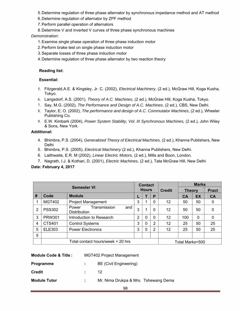
98
5. Determine regulation of three phase alternator by synchronous impedance method and AT method
6. Determine regulation of alternator by ZPF method
7. Perform parallel operation of alternators
8. Determine V and inverted V curves of three phase synchronous machines
Demonstration:
1. Examine single phase operation of three phase induction motor
2. Perform brake test on single phase induction motor
3. Separate losses of three phase induction motor
4. Determine regulation of three phase alternator by two reaction theory
Reading list:
Essential:
5. Fitzgerald,A.E. & Kingsley, Jr. C. (2002), Electrical Machinery, (2 ed.), McGraw Hill, Koga Kusha, Tokyo.
6. Langsdorf, A.S. (2001), Theory of A.C. Machines, (2 ed.), McGraw Hill, Koga Kusha, Tokyo.
7. Say, M.G. (2002), The Performance and Design of A.C. Machines, (2 ed.), CBS, New Delhi.
8. Taylor, E. O. (2002), The performance and design of A.C. Commutator Machines, (2 ed.), Wheeler Publishing Co.
9. E.W. Kimbark (2004), Power System Stability, Vol. III Synchronous Machines, (2 ed.), John Wiley & Sons, New York.
Additional:
4. Bhimbra, P.S. (2004), Generalized Theory of Electrical Machines, (2 ed.), Khanna Publishers, New Delhi
5. Bhimbra, P.S. (2005), Electrical Machinery (2 ed.), Khanna Publishers, New Delhi.
6. Laithwaite, E.R. M (2002), Linear Electric Motors, (2 ed.), Mills and Boon, London.
7. Nagrath, I.J. & Kothari, D. (2001), Electric Machines, (2 ed.), Tata McGraw Hill, New Delhi
Date: February 4, 2017
Semester VI Contact Hours Credit
Marks
Theory Pract # Code Module L T P CA EX CA 1 MGT402 Project Management 3 1 0 12 50 50 0
2 PSS302 Power Transmission and Distribution
3 1 0 12 50 50 0
3 PRW301 Introduction to Research 2 0 0 12 100 0 0
4 CTS401 Control Systems 3 0 2 12 25 50 25
5 ELE303 Power Electronics 3 0 2 12 25 50 25
5
Total contact hours/week = 20 hrs Total Marks=500
Module Code & Title : MGT402 Project Management
Programme : BE (Civil Engineering)
Credit : 12
Module Tutor : Mr. Nima Drukpa & Mrs. Tshewang Dema
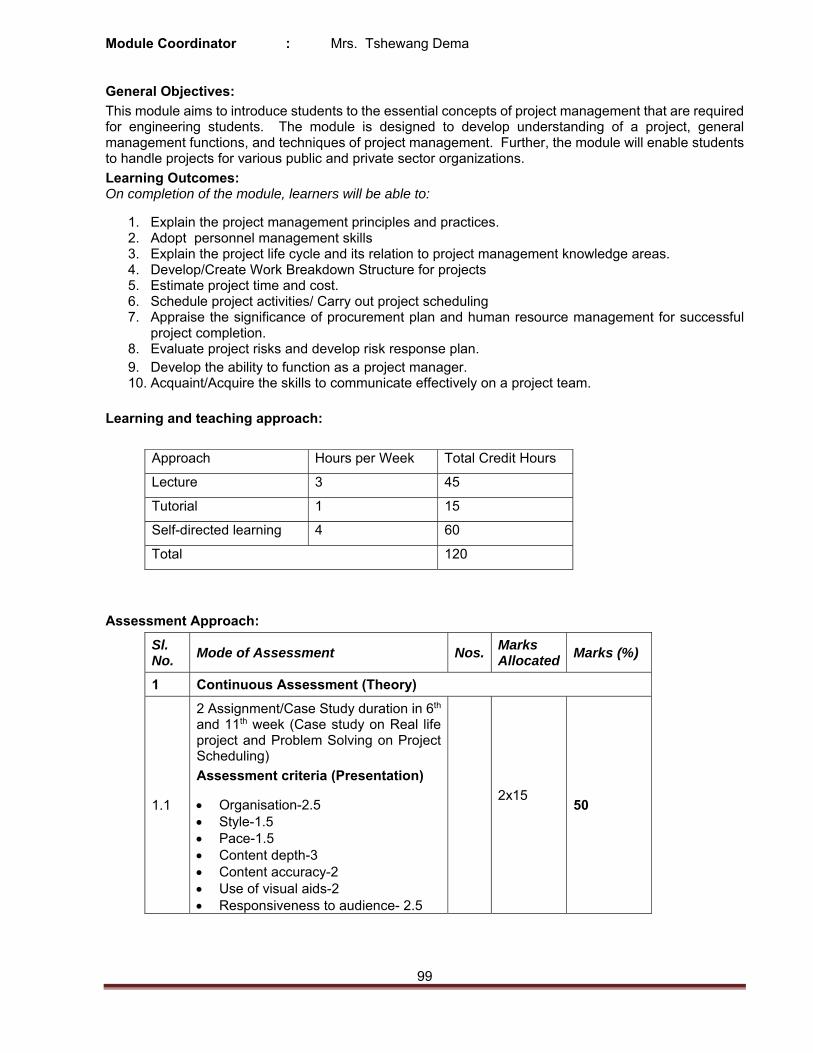
99
Module Coordinator : Mrs. Tshewang Dema
General Objectives:
This module aims to introduce students to the essential concepts of project management that are required for engineering students. The module is designed to develop understanding of a project, general management functions, and techniques of project management. Further, the module will enable students to handle projects for various public and private sector organizations.
Learning Outcomes: On completion of the module, learners will be able to:
1. Explain the project management principles and practices. 2. Adopt personnel management skills 3. Explain the project life cycle and its relation to project management knowledge areas. 4. Develop/Create Work Breakdown Structure for projects 5. Estimate project time and cost. 6. Schedule project activities/ Carry out project scheduling 7. Appraise the significance of procurement plan and human resource management for successful
project completion. 8. Evaluate project risks and develop risk response plan. 9. Develop the ability to function as a project manager. 10. Acquaint/Acquire the skills to communicate effectively on a project team.
Learning and teaching approach:
Approach Hours per Week Total Credit Hours
Lecture 3 45
Tutorial 1 15
Self-directed learning 4 60
Total 120
Assessment Approach:
Sl. No.
Mode of Assessment Nos.Marks Allocated
Marks (%)
1 Continuous Assessment (Theory)
1.1
2 Assignment/Case Study duration in 6th and 11th week (Case study on Real life project and Problem Solving on Project Scheduling)
Assessment criteria (Presentation)
Organisation-2.5 Style-1.5 Pace-1.5 Content depth-3 Content accuracy-2 Use of visual aids-2 Responsiveness to audience- 2.5
2x15
50
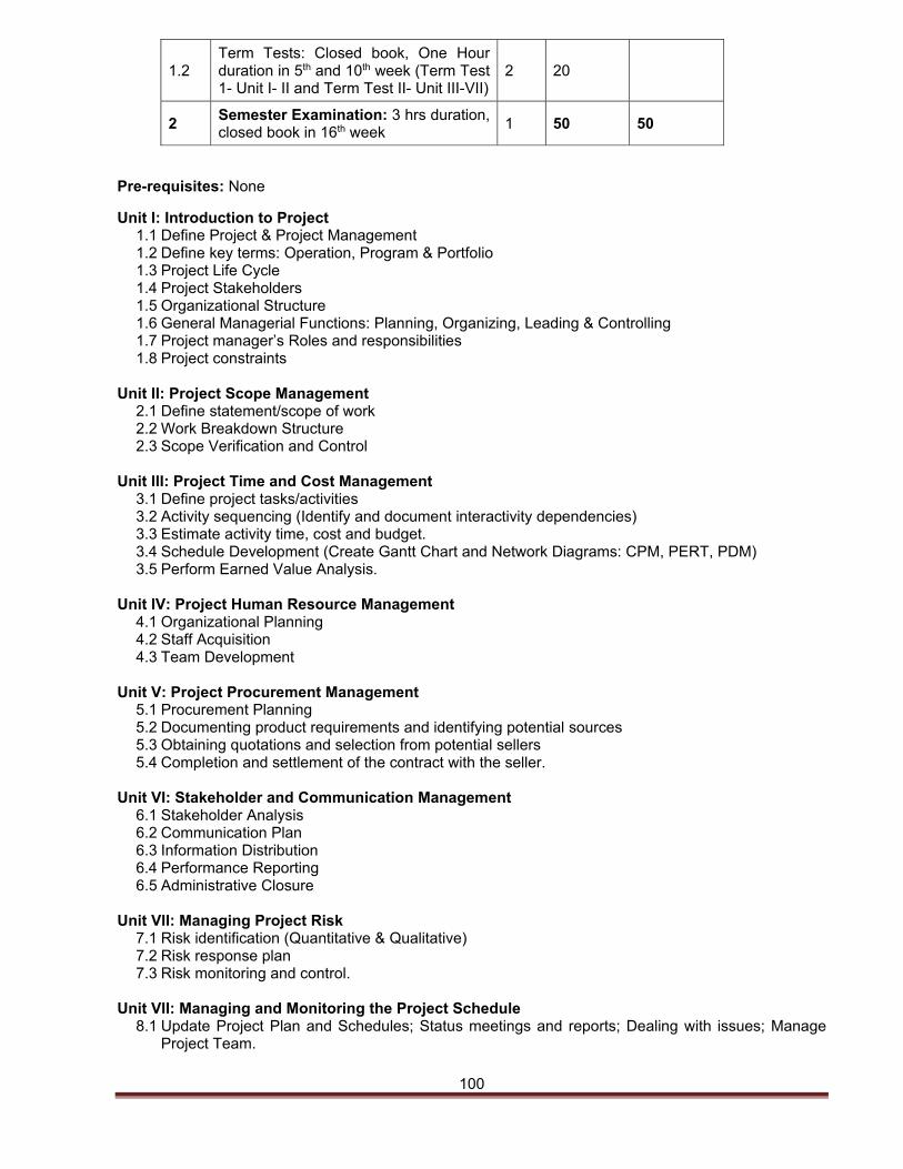
100
1.2 Term Tests: Closed book, One Hour duration in 5th and 10th week (Term Test 1- Unit I- II and Term Test II- Unit III-VII)
2 20
2 Semester Examination: 3 hrs duration, closed book in 16th week
1 50 50
Pre-requisites: None
Unit I: Introduction to Project 1.1 Define Project & Project Management 1.2 Define key terms: Operation, Program & Portfolio 1.3 Project Life Cycle 1.4 Project Stakeholders 1.5 Organizational Structure 1.6 General Managerial Functions: Planning, Organizing, Leading & Controlling 1.7 Project manager’s Roles and responsibilities 1.8 Project constraints
Unit II: Project Scope Management
2.1 Define statement/scope of work 2.2 Work Breakdown Structure 2.3 Scope Verification and Control
Unit III: Project Time and Cost Management
3.1 Define project tasks/activities 3.2 Activity sequencing (Identify and document interactivity dependencies) 3.3 Estimate activity time, cost and budget. 3.4 Schedule Development (Create Gantt Chart and Network Diagrams: CPM, PERT, PDM) 3.5 Perform Earned Value Analysis.
Unit IV: Project Human Resource Management
4.1 Organizational Planning 4.2 Staff Acquisition 4.3 Team Development
Unit V: Project Procurement Management
5.1 Procurement Planning 5.2 Documenting product requirements and identifying potential sources 5.3 Obtaining quotations and selection from potential sellers 5.4 Completion and settlement of the contract with the seller.
Unit VI: Stakeholder and Communication Management
6.1 Stakeholder Analysis 6.2 Communication Plan 6.3 Information Distribution 6.4 Performance Reporting 6.5 Administrative Closure
Unit VII: Managing Project Risk
7.1 Risk identification (Quantitative & Qualitative) 7.2 Risk response plan 7.3 Risk monitoring and control.
Unit VII: Managing and Monitoring the Project Schedule
8.1 Update Project Plan and Schedules; Status meetings and reports; Dealing with issues; Manage Project Team.
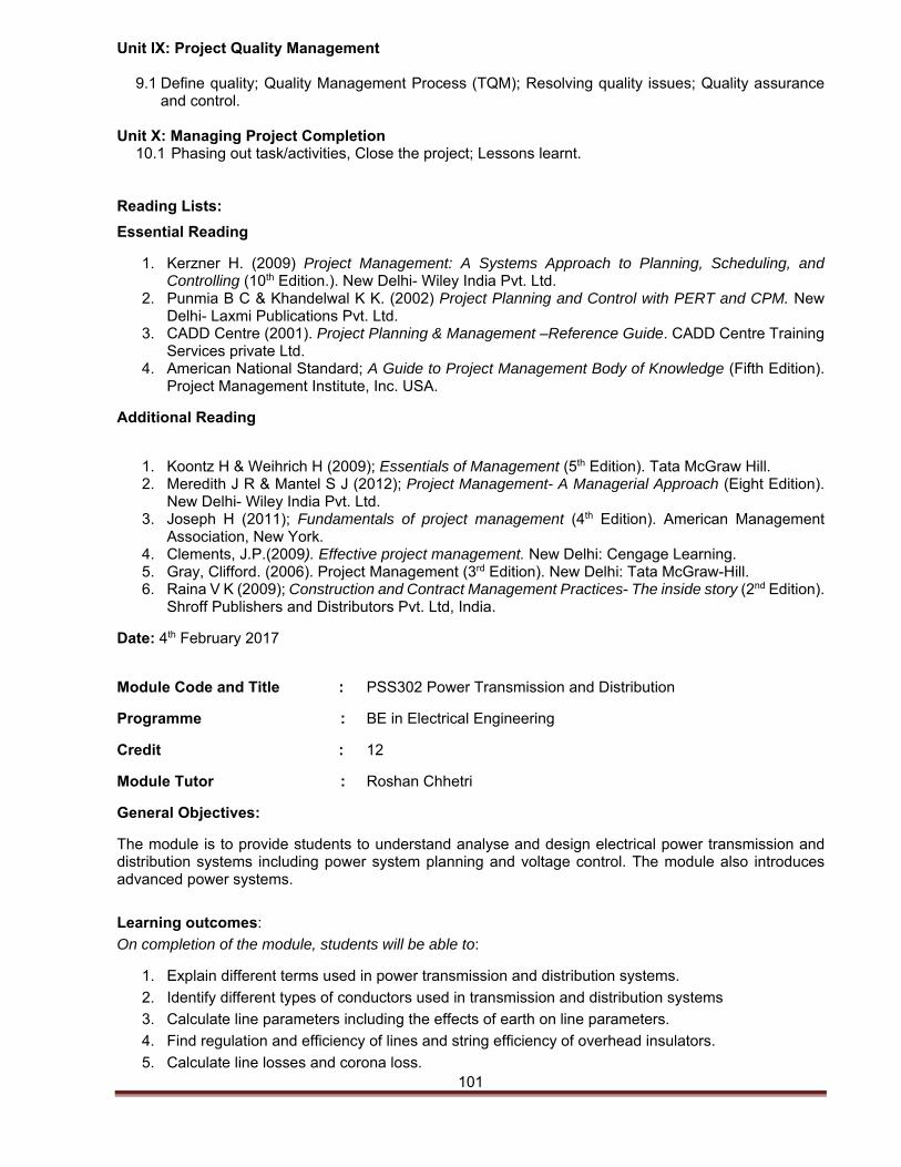
101
Unit IX: Project Quality Management
9.1 Define quality; Quality Management Process (TQM); Resolving quality issues; Quality assurance and control.
Unit X: Managing Project Completion
10.1 Phasing out task/activities, Close the project; Lessons learnt. Reading Lists:
Essential Reading
1. Kerzner H. (2009) Project Management: A Systems Approach to Planning, Scheduling, and Controlling (10th Edition.). New Delhi- Wiley India Pvt. Ltd.
2. Punmia B C & Khandelwal K K. (2002) Project Planning and Control with PERT and CPM. New Delhi- Laxmi Publications Pvt. Ltd.
3. CADD Centre (2001). Project Planning & Management –Reference Guide. CADD Centre Training Services private Ltd.
4. American National Standard; A Guide to Project Management Body of Knowledge (Fifth Edition). Project Management Institute, Inc. USA.
Additional Reading
1. Koontz H & Weihrich H (2009); Essentials of Management (5th Edition). Tata McGraw Hill. 2. Meredith J R & Mantel S J (2012); Project Management- A Managerial Approach (Eight Edition).
New Delhi- Wiley India Pvt. Ltd. 3. Joseph H (2011); Fundamentals of project management (4th Edition). American Management
Association, New York. 4. Clements, J.P.(2009). Effective project management. New Delhi: Cengage Learning. 5. Gray, Clifford. (2006). Project Management (3rd Edition). New Delhi: Tata McGraw-Hill. 6. Raina V K (2009); Construction and Contract Management Practices- The inside story (2nd Edition).
Shroff Publishers and Distributors Pvt. Ltd, India.
Date: 4th February 2017
Module Code and Title : PSS302 Power Transmission and Distribution
Programme : BE in Electrical Engineering
Credit : 12
Module Tutor : Roshan Chhetri
General Objectives:
The module is to provide students to understand analyse and design electrical power transmission and distribution systems including power system planning and voltage control. The module also introduces advanced power systems.
Learning outcomes:
On completion of the module, students will be able to:
1. Explain different terms used in power transmission and distribution systems.
2. Identify different types of conductors used in transmission and distribution systems
3. Calculate line parameters including the effects of earth on line parameters.
4. Find regulation and efficiency of lines and string efficiency of overhead insulators.
5. Calculate line losses and corona loss.
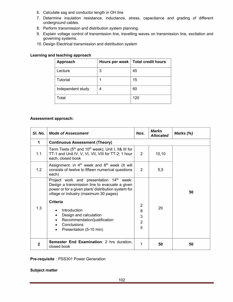
102
6. Calculate sag and conductor length in OH line
7. Determine insulation resistance, inductance, stress, capacitance and grading of different underground cables.
8. Perform transmission and distribution system planning.
9. Explain voltage control of transmission line, travelling waves on transmission line, excitation and governing systems.
10. Design Electrical transmission and distribution system
Learning and teaching approach
Approach Hours per week Total credit hours
Lecture 3 45
Tutorial 1 15
Independent study 4 60
Total 120
Assessment approach:
Pre-requisite : PSS301 Power Generation
Subject matter
Sl. No. Mode of Assessment Nos. Marks Allocated
Marks (%)
1 Continuous Assessment (Theory)
1.1 Term Tests (5th and 10th week); Unit I, II& III for TT-1 and Unit IV, V, VI, VII, VIII for TT-2; 1 hour each, closed book
2 10,10
50
1.2 Assignment: in 4th week and 8th week (It will consists of twelve to fifteen numerical questions each)
2 5,5
1.3
Project work and presentation 14th week: Design a transmission line to evacuate a given power or for a given plant/ distribution system for village or industry (maximum 30 pages)
Criteria
Introduction Design and calculation Recommendation/justification Conclusions Presentation (5-10 min)
2
8
3
2
5
20
2 Semester End Examination: 2 hrs duration, closed book
1 50 50
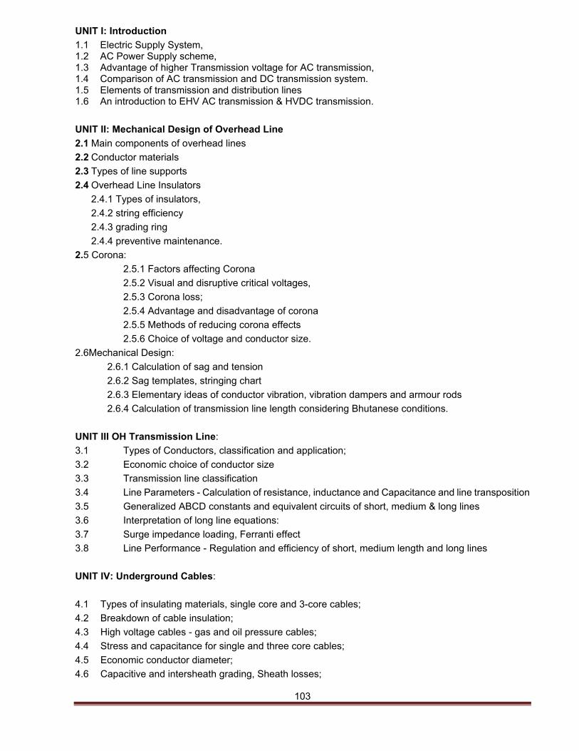
103
UNIT I: Introduction
1.1 Electric Supply System, 1.2 AC Power Supply scheme, 1.3 Advantage of higher Transmission voltage for AC transmission, 1.4 Comparison of AC transmission and DC transmission system. 1.5 Elements of transmission and distribution lines 1.6 An introduction to EHV AC transmission & HVDC transmission.
UNIT II: Mechanical Design of Overhead Line
2.1 Main components of overhead lines
2.2 Conductor materials
2.3 Types of line supports
2.4 Overhead Line Insulators
2.4.1 Types of insulators,
2.4.2 string efficiency
2.4.3 grading ring
2.4.4 preventive maintenance.
2.5 Corona:
2.5.1 Factors affecting Corona
2.5.2 Visual and disruptive critical voltages,
2.5.3 Corona loss;
2.5.4 Advantage and disadvantage of corona
2.5.5 Methods of reducing corona effects
2.5.6 Choice of voltage and conductor size.
2.6Mechanical Design:
2.6.1 Calculation of sag and tension
2.6.2 Sag templates, stringing chart
2.6.3 Elementary ideas of conductor vibration, vibration dampers and armour rods
2.6.4 Calculation of transmission line length considering Bhutanese conditions.
UNIT III OH Transmission Line:
3.1 Types of Conductors, classification and application;
3.2 Economic choice of conductor size
3.3 Transmission line classification
3.4 Line Parameters - Calculation of resistance, inductance and Capacitance and line transposition
3.5 Generalized ABCD constants and equivalent circuits of short, medium & long lines
3.6 Interpretation of long line equations:
3.7 Surge impedance loading, Ferranti effect
3.8 Line Performance - Regulation and efficiency of short, medium length and long lines
UNIT IV: Underground Cables:
4.1 Types of insulating materials, single core and 3-core cables;
4.2 Breakdown of cable insulation;
4.3 High voltage cables - gas and oil pressure cables;
4.4 Stress and capacitance for single and three core cables;
4.5 Economic conductor diameter;
4.6 Capacitive and intersheath grading, Sheath losses;
104
4.7 Condenser bushing, Thermal characteristics;
4.8 Methods of laying cables;
4.9 Cables for direct current transmission.
UNIT V: AC Distribution System:
5.1 Classification,
5.2 requirement of Distribution system, Primary and secondary distribution system
5.3 comparison of UG and OH
5.4 Voltage drop and power loss calculations,
UNIT VI: Voltage Control:
6.1 Tap changing transformer, phase control, booster transformers and phase shifting transformer;
6.2 Series and shunt compensations;
6.3 Location and protection of series capacitors, advantages and problems
UNIT VII: Grounding System:
7.1 Importance of grounding in a substation
7.2 Ungrounded system and effective grounded system;
7.3 Resistance, reactance and resonant grounded systems, and their merits and demerits.
UNIT VIII: Transmission System and Distribution System Planning:
8.1 Criterion for transmission planning;
8.2 Economic and reliability consideration, Methods of planning;
8.3 Criterion for distribution planning;
8.4 Various distribution strategies for rural and urban systems.
UNIT IX: Travelling Waves:
9.1 Travelling waves on transmission lines;
9.2 Wave equations and specification of travelling waves;
9.3 Reflection and refraction of travelling waves;
9.4 typical cases of line terminations.
UNIT X: Substation Equipment:
10.1 Classification, functions and major components of substations
10.2 Busbar arrangements and sub-station layout
10.3 Distribution sub-station bus-bar connections, Isolators, shielding, earthing and earth electrodes, Location of C.Ts and PTs , Earthing mat.
Note: Project work- to include one of the following area:
1. Electrical design of transmission lines.
2. Planning and design of town/village electrification schemes.
3. Design of industrial distribution systems.
Reading lists:
Essential reading
1. Nagrath, J., Kothari, D.P. (2003). Power System Engineering, New Delhi:Tata Mc Graw Hill.
2. Wadhwa, C. L. (2003). Electrical Power System, New Delhi: New Age International.
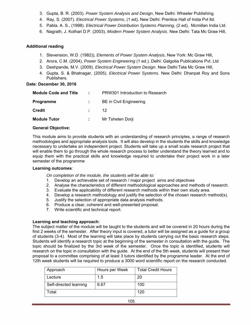
105
3. Gupta, B. R. (2003). Power System Analysis and Design, New Delhi: Wheeler Publishing.
4. Ray, S. (2007). Electrical Power Systems, (1 ed), New Delhi: Prentice Hall of Inida Pvt ltd.
5. Pabla. A. S., (1998). Electrical Power Distribution Systems Planning, (2 ed), Mcmillan India Ltd.
6. Nagrath, J. Kothari D.P. (2003), Modern Power System Analysis. New Delhi: Tata Mc Graw Hill,
Additional reading
1. Stevension, W.D. (1982)), Elements of Power System Analysis, New York: Mc Graw Hill,
2. Arora, C.M. (2004), Power System Engineering (1 ed.). Delhi: Galgotia Publications Pvt. Ltd
3. Deshpande, M.V. (2009). Electrical Power System Design. New Delhi:Tata Mc Graw Hill,
4. Gupta, S. & Bhatnagar, (2005). Electrical Power Systems. New Delhi: Dhanpat Roy and Sons Publishers.
Date: December 30, 2016
Module Code and Title : PRW301 Introduction to Research
Programme : BE in Civil Engineering
Credit : 12
Module Tutor : Mr Tsheten Dorji
General Objective:
This module aims to provide students with an understanding of research principles, a range of research methodologies and appropriate analysis tools. It will also develop in the students the skills and knowledge necessary to undertake an independent project. Students will take up a small scale research project that will enable them to go through the whole research process to better understand the theory learned and to equip them with the practical skills and knowledge required to undertake their project work in a later semester of the programme
Learning outcomes:
On completion of the module, the students will be able to: 1. Develop an achievable set of research / major project aims and objectives 2. Analyse the characteristics of different methodological approaches and methods of research. 3. Evaluate the applicability of different research methods within their own study area. 4. Develop a research methodology and justify the selection of the chosen research method(s). 5. Justify the selection of appropriate data analysis methods. 6. Produce a clear, coherent and well-presented proposal. 7. Write scientific and technical report.
Learning and teaching approach: The subject matter of the module will be taught to the students and will be covered in 20 hours during the first 2 weeks of the semester. After theory input is covered, a tutor will be assigned as a guide for a group of students (3-4). Most of the learning will take place by students carrying out the basic research steps. Students will identify a research topic at the beginning of the semester in consultation with the guide. The topic should be finalized by the 3rd week of the semester. Once the topic is identified, students will research on the topic in consultation with the guide. At the end of the 5th week, students will present their proposal to a committee comprising of at least 3 tutors identified by the programme leader. At the end of 12th week students will be required to produce a 3000 word scientific report on the research conducted.
Approach Hours per Week Total Credit Hours
Lecture 1.5 20
Self-directed learning 6.67 100
Total 120
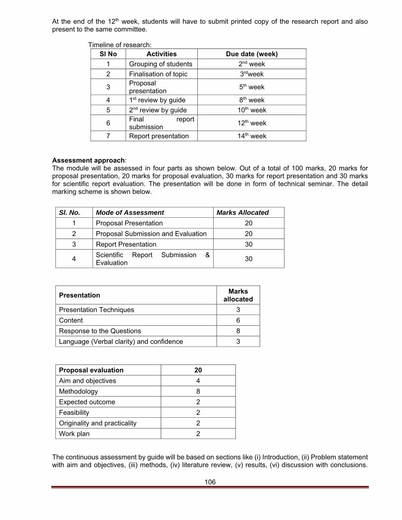
106
At the end of the 12th week, students will have to submit printed copy of the research report and also present to the same committee. Timeline of research:
Sl No Activities Due date (week)
1 Grouping of students 2nd week
2 Finalisation of topic 3rdweek
3 Proposal presentation
5th week
4 1st review by guide 8th week
5 2nd review by guide 10th week
6 Final report submission
12th week
7 Report presentation 14th week
Assessment approach: The module will be assessed in four parts as shown below. Out of a total of 100 marks, 20 marks for proposal presentation, 20 marks for proposal evaluation, 30 marks for report presentation and 30 marks for scientific report evaluation. The presentation will be done in form of technical seminar. The detail marking scheme is shown below.
Sl. No. Mode of Assessment Marks Allocated
1 Proposal Presentation 20
2 Proposal Submission and Evaluation 20
3 Report Presentation 30
4 Scientific Report Submission & Evaluation
30
Presentation Marks
allocated
Presentation Techniques 3
Content 6
Response to the Questions 8
Language (Verbal clarity) and confidence 3
Proposal evaluation 20
Aim and objectives 4
Methodology 8
Expected outcome 2
Feasibility 2
Originality and practicality 2
Work plan 2
The continuous assessment by guide will be based on sections like (i) Introduction, (ii) Problem statement with aim and objectives, (iii) methods, (iv) literature review, (v) results, (vi) discussion with conclusions.
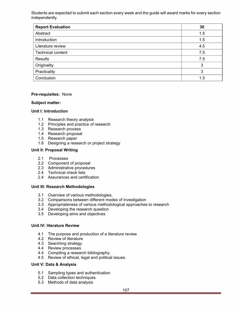
107
Students are expected to submit each section every week and the guide will award marks for every section independently.
Report Evaluation 30
Abstract 1.5
Introduction 1.5
Literature review 4.5
Technical content 7.5
Results 7.5
Originality 3
Practicality 3
Conclusion 1.5
Pre-requisites: None
Subject matter:
Unit I: Introduction
1.1 Research theory analysis 1.2 Principles and practice of research 1.3 Research process 1.4 Research proposal 1.5 Research paper 1.6 Designing a research or project strategy
Unit II: Proposal Writing
2.1 Processes 2.2 Component of proposal 2.3 Administrative procedures 2.4 Technical check lists 2.4 Assurances and certification
Unit III: Research Methodologies
3.1 Overview of various methodologies, 3.2 Comparisons between different modes of investigation 3.3 Appropriateness of various methodological approaches to research 3.4 Developing the research question 3.5 Developing aims and objectives
Unit IV: literature Review
4.1 The purpose and production of a literature review 4.2 Review of literature 4.3 Searching strategy 4.4 Review processes 4.4 Compiling a research bibliography. 4.5 Review of ethical, legal and political issues.
Unit V: Data & Analysis
5.1 Sampling types and authentication 5.2 Data collection techniques 5.3 Methods of data analysis
108
5.4 Evaluation of analysis tools 5.5 Interpreting the results of data analysis 5.6 Presentation and Interpretation of result
Unit VI Referencing System
6.1 Type of referencing and citation 6.2 Referencing and citation system 6.3 Table, Figure and formula citation
Unit VII Report and Publication
7.1 Accurate documentation 7.2 Abstract, introduction, methods, literature review, result discussion and conclusion. 7.3 Publication process
Reading List: Essential Reading:
1. Balnaves, M. & Caputi, P. (2001).Introduction to Quantitative Research Methods: An investigative approach, Sage Publications Ltd., London.
2. Hart, C (1998).Doing a Literature Review, Sage Publications Ltd., London. 3. Ruane J M (2005). Essentials of Research Methods: A Guide to Social Science Research, Wiley-
Blackwell Publishing, London. 4. Punch K.F. (2006). Developing Effective Research Proposals (Essential Resource Books for Social
Research) (2nd edition), Sage Publications Ltd., London. Additional Reading:
1. Plowright, D. (2011) Using Mixed Methods: frameworks for an integrated ethodology, Sage Publications Ltd., London.
2. Yin, R. (2009) Case Study Research: Design and Methods (4th edition.), Sage Publications Ltd., London.
Date: March 26, 2016
Module Code and Title : CTS401Control Systems Programme : BE in Electrical Engineering Credit Value : 12 Module Tutor : Mr. Manoj Sharma
General objectives: This module will introduce the fundamental principles of analysis and design of control systems using linear methods; time and frequency responses.The experiments will familiarize actual control techniques with hardware systems. Learning outcomes: On completion of the module, students will be able to:
1. Analyse open loop and the effect of feedback on a system. 2. Construct physical static and dynamic systems. 3. Design mathematical modeling of dynamic systems 4. Select and analyse time response specifications, performance Index of a control system. 5. Analyse frequency response specifications, performance Index of a control system. 6. Calculate steady-state error specifications of a control system. 7. Design compensators, controllers through root locus design and frequency response
techniques; 8. State Models of linear systems, transfer function to state space and vice-versa. 9. Analyse and distinguish Z-Transform Function. 10. Perform Inverse Z-Transform Function.
109
Learning and teaching approach:
Approach Hours per Week
Total Credit Hours
Lecture 3 45 Practical 2 30 Independent study/self-directed learning 3 45 Total 120
Assessment approach:
Sl. No. Mode of Assessment Nos. Marks Allocated
Marks (%)
1 Continuous Assessment (Theory) 25%
1.1
Term Tests: Closed book, one hour duration in 5th and 10th week.
Two units will be covered for term I and three for term II.
2 20
25
1.2 Assignments; at the end of 3rd and 8th week.
2 2.5, 2.5
2 Continuous Assessment (Practical) 25%
2.1
Regular Practical Assessments
Assessment Criteria(Report)
Introduction Materials and Methods Results Discussion Conclusion
10
10
1
2.5
2.5
3
1
25
2.2 Practical Exam 1 10
2.3 Viva Voce 1 5
3 Semester Examination (Closed book 3 hours) 50%
1 50 50
Pre-requisites: MAT208 Engineering Mathematics-IV Subject Matter:
Unit I: Introduction
1.1. System identification 1.1.1. Concept and basic configuration 1.1.2. Differentiate between mathematical modelling and system identification 1.1.3. Methods; Parametric approach, Nonparametric approach
1.2. Basic components of a control system 1.2.1. Concept and configuration of a control system 1.2.2. Process; Setpoint, Manipulated variable, Controlled variable 1.2.3. Controller 1.2.4. Comparator 1.2.5. Feedback elements
110
1.3. Types of control systems 1.3.1. Open-loop control systems 1.3.2. Feedback control systems 1.3.3. Multivariable control systems 1.3.4. Servo and Regulator systems 1.3.5. Linear and Non-linear control systems 1.3.6. Time variant and Time invariant control system 1.3.7. Lumped parameter and Distributed parameter control systems 1.3.8. Continuous data and discrete time control system 1.3.9. Deterministic and Stochastic control system 1.3.10. Static and Dynamic control system 1.3.11. Adaptive Control System.
1.4. Effects of feedback 1.4.1. Feedback control system 1.4.2. Feedforward control system 1.4.3. Differentiate between feedforward and feedback control system
Unit II: Transfer Function
2.1. Laplace transform 2.1.1. Transform Ordinary Differential Equations to frequency domain 2.1.2. Partial fraction expansion 2.1.3. Tables of Laplace transforms 2.1.4. Properties of Laplace transform 2.1.5. The Final Value Theorem
2.2. System transfer functions (SISO) 2.2.1. Poles and zeros 2.2.2. S-plane 2.2.3. Transfer function of an open loop and a closed loop systems.
2.3. Dynamic models; State space model 2.4. Block diagrams (reduction of multiple subsystem)
2.4.1. Combining block in Cascade 2.4.2. Moving a summing point behind a block 2.4.3. Moving a pickoff point ahead of a block 2.4.4. Moving a pickoff point beyond a block 2.4.5. Moving a summing point ahead of a block 2.4.6. Eliminating a forward loop. 2.4.7. Eliminating a feedback loop.
2.5. Physical system modeling 2.5.1. Electrical 2.5.2. Mechanical or 2.5.3. Electromechanical systems
Unit III: System Analysis
3.1. Effects of Poles and zeros 3.1.1. Poles and zeros at negative real axis. 3.1.2. Poles and zeros at origin. 3.1.3. Poles and zeros at positive real axis.
3.2. Test Signals or Excitation Functions 3.2.1. Impulse signal 3.2.2. Step signal 3.2.3. Ramp signal 3.2.4. Parabolic signal
3.3. Order of the System 3.4. Type of Systems 3.5. First order systems
3.5.1. Response to unit step function. 3.5.2. Effect of pole of the input function. 3.5.3. First order system specifications.
111
3.5.4. Response to unit ramp input. 3.6. Second order systems
3.6.1. Behaviour of second order systems 3.6.2. Solution of second order system equation 3.6.3. Response to unit step input : Critically damped 3.6.4. Under-damped second order systems 3.6.5. Response to unit step input : Undamped & overdamped. 3.6.6. Time Response Specifications (Performance Index) 3.6.7. Step responses to additional poles. 3.6.8. Effect of zeros on time response.
3.7. Response of higher order systems 3.8. Stability (Routh-Hurwitz criterion)
3.8.1. Necessary and sufficient conditions 3.8.2. Limitations 3.8.3. Special Cases
Unit IV: Error Analysis
4.1. Analysis of steady-state errors 4.1.1. Evaluation of steady state error.
4.2. Error constants and system types 4.2.1. Relationship between input, system type, static error constants, and steady-state
errors. 4.3. Steady-state error specifications
4.3.1. Static error constants. 4.3.2. Sensitivity
Unit V: Stability of Systems:
5.1. Root locus of a basic feedback system 5.2. Rules for sketching the root locus
5.2.1. Symmetry about the real axis. 5.2.2. Number of branches 5.2.3. Starting and ending point 5.2.4. Locus on the real axis. 5.2.5. Behaviour at infinity 5.2.6. Determination of Break away and break in-points. 5.2.7. Determination of departure from complex poles. 5.2.8. Determination of arrival at complex zeros. 5.2.9. Determination of locus crossing imaginary axis.
5.3. Compensator/controller design 5.3.1. Understanding the problem of root locus design 5.3.2. Phase Lead compensation design. 5.3.3. Phase Lag compensation design. 5.3.4. Lead-lag compensation design.
Unit VI: Frequency of Systems:
6.1. Frequency response of a closed-loop system 6.2. Frequency-Domain Specifications 6.3. Bode Plot
6.3.1. Magnitude and phase angle curves. 6.3.2. Straight line approximation 6.3.3. Corner frequency 6.3.4. General procedure for constructing Bode plots. 6.3.5. Assessment of stability.
6.4. Effects of adding zeros and poles in the forward path transfer function 6.5. Nyquist stability
6.5.1. Principle 6.5.2. Nyquist path 6.5.3. Nyquist stability criteria
112
6.5.4. Determination of stability 6.5.5. Assessment of Nyquist stability 6.5.6. Gain margin and phase margin.
6.6. Nichols chart 6.7. Design by frequency response methods
6.7.1. Frequency domain interpretation of Phase lead control. 6.7.2. Frequency domain interpretation and design of Phase Lag Control 6.7.3. Frequency domain interpretation and design of Lead lag control.
Unit VII: PID controls:
7.1. Tuning rules for PID controllers; 7.1.1. PID controller tuning using Ziegler-Nichols technique 7.1.2. PID Controller tuning using the Process Reaction curve or Cohen-Coon Method.
7.2. Modifications of PID control schemes.
Unit VIII: State Models: 8.1. Converting a transfer function to state space 8.2. Converting from state space to a transfer function 8.3. Eigen Values and Eigen Vectors 8.4. Similarity transformation
8.4.1. Properties of similarity transformations 8.4.2. Controllability Canonical Form 8.4.3. Observability Canonical form 8.4.4. Diagonal Canonical Form 8.4.5. Jordan Canonical Form
8.5. Decomposition of transfer functions 8.5.1. Direct Decomposition 8.5.2. Cascade Decomposition. 8.5.3. Parallel Decomposition.
8.6. Controllability and Observability of linear systems 8.6.1. General concept of controllability 8.6.2. Definition of state Controllability 8.6.3. Alternate tests on controllability. 8.6.4. Definition of Observability 8.6.5. Alternate tests on observability.
Unit IX: Digital Control System:
9.1. The z-transform 9.1.1. Properties of Z-Transform 9.1.2. The Z Transfer Function (Pulse Transfer Function)
9.2. The Inverse Z-Transform 9.3. Z and S Domain Relationship.
List of Practical: 1. Experiment dynamic response of 1st and 2nd order systems. 2. Operate and demonstrate P Controller for 1st order system. 3. Operate and demonstrate PI, PD, and PID Control for 1st order system. 4. Operate and demonstrate PID Controller for 2nd order system. 5. Practice and experiment PID parameter tuning with Zieglar Nichols 1st method. 6. Practice and experiment PID parameter tuning with Zieglar Nichols 2nd method. 7. Designing linear systems and P-Controller with OP-Amps . 8. Designing interlocks or sequential control with digital ICs. 9. Obtain the state space representation in different canonical forms for a given system. 10. To check whether the system is observable or controllable using Kalman’s method.
Reading list: Essential Reading
113
1. Nise, N. S. (2004). Control Systems Engineering. (4 ed.). New Delhi: Wiley. 2. Kuo, B, C. &. Golnaraghi, F. (2002). Automatic Control Systems. (8 ed.). New Delhi. Wiley. 3. Katsuhiko, O. (2004). Modern Control Engineering. (4 ed.). New Delhi. Prentice Hall of India. PHI
Private Limited. 4. Bolton, W. (2003). Mechatronics. (5 ed.). Singapore. Pearson Education. Delhi.. Pte. Ltd.Indian
Branch. 5. IEC (International Electrotechnical Commission) Standard 61511, Functional Safety: Safety
Instrumented System for Process Industry Sector. 6. Gibson &. Tuteur. (2003). Control System Components. (2 ed.). Singapore: McGraw Hill..
Additonal Reading
1. Dorf, R. C. & Bishop, R, H. (2002). Modern Control Systems. (8 ed.), Singapore. Pearson
Education. 2. Wolf, S. &. Smith, R. F.AM. (2005). Student Reference Manual for Electronic Instrumentation
Laboratories. New Delhi: Prentice-Hall of India, Private Limited. 3. Martin, M. W. & Schinzinger, R. (2003). Ethics in Engineering. (4 ed.). New York: Tata McGraw-
Hill,. 4. Nagrath, I. J. &. Gopal, M (1999). Control System Engineering. (5 ed.). New Delhi: Willey Eastern.
Date: September 26, 2016
Module Code and Title : ELE303 Power Electronics Programme : BE in Electrical Engineering Credit : 12 Module Tutor : Sonam Norbu
General Objective:
This module will familiarize students with the concept of power electronics dealing with switching and power conversion applications. This module will also facilitate students with concept of working principle of various types of converters applicable in electrical engineering.
Learning outcomes:
On completion of the module, students will be able to:
1. Explain the principles of power converters. 2. Design the semiconductor devices for switching applications and power conversion applications. 3. Distinguish different types of power converters 4. Analyse the operation of power converters. 5. Design the power converters. 6. Analyse the power converters. 7. Specify power converters for various applications. 8. Design heat sinks, snubber circuits and gate drive requirements for different power converters.
Learning and teaching approach:
Approach Hours per Week Total Credit Hours
Lecture 3 45
Practical 2 30
Independent study 3 45
Total 120
Assessment approach:
114
Sl. No. Mode of Assessment Nos. Marks Allocated
Marks (%)
1 Continuous Assessment (Theory) 25%
1.1
Term Tests: Closed book, one hour duration in 5th and 10th week.
Two units will be covered for term I and three for term II.
2 20
25
1.2 Assignments; at the end of 3rd and 8th week.
2 2.5, 2.5
2 Continuous Assessment (Practical) 25%
2.1
Regular Practical Assessments
Assessment Criteria(Report)
Introduction Materials and Methods Results Discussion Conclusion
10
1
2.5
2.5
3
1
10
25
2.2 Practical Exam 1 10
2.3 Viva Voce 1 5
3 Semester Examination (Closed book 3 hours)
1 50 50
Pre-requisites:- ELE101Electronics I and ELE202 Electronics II
Subject matter:
Unit I: Introduction:
1.1 Concept of power electronics, scope and applications
1.2 Types of power converters
1.3 Types of power semiconductors switches
1.2 V-I Characteristics – Diodes, SCR, TRIAC, Power BJT, POWER MOSFET, IGBT
Unit II: AC-DC Converters:
2.1 Rectifiers: Introduction, Diode - Passive rectifiers
2.2 Principles of phase controlled converters operation
2.3 Single and Three phase controlled converters
2.4 Analysis with and without freewheeling diode of R, R-L, and RLC load
2.5 Single phase and three phase dual converters
2.6 Effect of load and source inductances
2.7 General idea of gating circuits
Unit III: DC-DC Converters:
3.1 Introduction
3.2 Types and circuit configurations (buck, boost, buck/boost, cuk, converters with transformers)
3.3 Principles of operation and properties,
3.4 Advantages and disadvantages.
Unit IV: DC-AC Converters (Inverters):
4.1 Introduction
115
4.2 Single phase and three phase inverters with PWM and square wave operation
4.3 Uni-polar and Bi-polar mode of operation
4.4 Ripples and harmonic distortions in inverters with various operating modes
Unit V: AC-AC Converters:
5.1 Single-phase and Three-phase ac-ac voltage controllers
5.2 Single-phase to Single-phase
5.3Three-phase to single-phase and three-phase to three-phase configurations of Cycloconverters,
5.4 Basics of Matrix converters
Unit VI: Auxiliary Circuits and Applications:
6.1 Heat sinks
6.2 Snubber circuits
6.3 Gate drive circuits
6.4 Design of Magnetic Components
6.5 Home appliances such as Induction Heating
6.6 Inverter air conditioner and Lighting,
6.7 Power electronics uses in Electric Vehicles,
6.8 Power electronics applications in Motor speed control, Uninterruptible Power Source (UPS), Constant Voltage Constant Frequency UPS, Solar power generation, and Direct Current power transmission.
List of Experiments
1. Study the characteristics of SCR, TRIAC and UJT 2. study the UJT as a Pulse Generator / Trigger source. 3. To study and fabricate the SCR triggering circuits and obtain AC phase control using resistance
triggering. 4. To study and fabricate the SCR triggering circuits and obtain AC phase control using UJT triggering
circuits. 5. To study and fabricate the TRIAC and DIAC triggering circuits and obtain AC phase control.
6. study the operation of a single phase fully controlled converter with R, R-L and RLC load 7. study symmetrical and asymmetrical single phase half controlled converter with R, RL and RLC loads 8. Design and analyze the operation of single phase AC voltage controller 9. Design and analyze the operation of Three phase fully controlled converter 10. Design and analyze the operation of three phase half controlled converter 11. study the operation of operation of single phase two stage sequence controller 12. study the operation of DC to Dc converter 13. study the operation of Single phase PWM inverter 14. study the operation of Single phase PWM converter. 15. Modelling and simulation of single phase haf controlled bridge rectifier with R,RL and RLE loads. 16. Modelling and simulation of single phase full bridge voltage source inverter. 17. Modelling and simulation of single phase AC voltage controller with R and RL load.
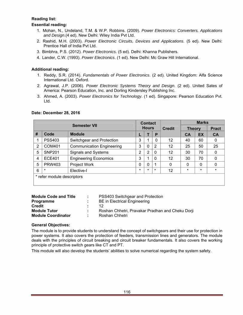
116
Reading list:
Essential reading:
1. Mohan, N., Undeland, T.M. & W.P. Robbins. (2009). Power Electronics: Converters, Applications and Design.(4 ed). New Delhi: Wiley India Pvt Ltd.
2. Rashid, M.H. (2003). Power Electronic Circuits, Devices and Applications. (5 ed). New Delhi: Prentice Hall of India Pvt Ltd.
3. Bimbhra, P.S. (2012). Power Electronics. (5 ed). Delhi: Khanna Publishers.
4. Lander, C.W. (1993). Power Electronics. (1 ed). New Delhi: Mc Graw Hill International.
Additional reading:
1. Reddy, S.R. (2014). Fundamentals of Power Electronics. (2 ed). United Kingdom: Alfa Science International Ltd. Oxford.
2. Agrawal, J.P. (2006). Power Electronic Systems Theory and Design. (2 ed). United Sates of America: Pearson Education, Inc. and Dorling Kindersley Publishing Inc.
3. Ahmed, A. (2003). Power Electronics for Technology. (1 ed). Singapore: Pearson Education Pvt. Ltd.
Date: December 28, 2016
Semester VII Contact Hours Credit
Marks
Theory Pract # Code Module L T P CA EX CA 1 PSS403 Switchgear and Protection 3 1 0 12 40 60 0
2 COM401 Communication Engineering 3 0 2 12 25 50 25
5 SNP201 Signals and Systems 2 2 0 12 30 70 0
4 ECE401 Engineering Economics 3 1 0 12 30 70 0
5 PRW403 Project Work 0 0 1 0 0 0 0
6 * Elective-I * * * 12 * * *
* refer module descriptors
Module Code and Title : PSS403 Switchgear and Protection Programme : BE in Electrical Engineering Credit : 12 Module Tutor : Roshan Chhetri, Pravakar Pradhan and Cheku Dorji Module Coordinator : Roshan Chhetri General Objectives:
The module is to provide students to understand the concept of switchgears and their use for protection in power systems. It also covers the protection of feeders, transmission lines and generators. The module deals with the principles of circuit breaking and circuit breaker fundamentals. It also covers the working principle of protective switch gears like CT and PT.
This module will also develop the students’ abilities to solve numerical regarding the system safety.
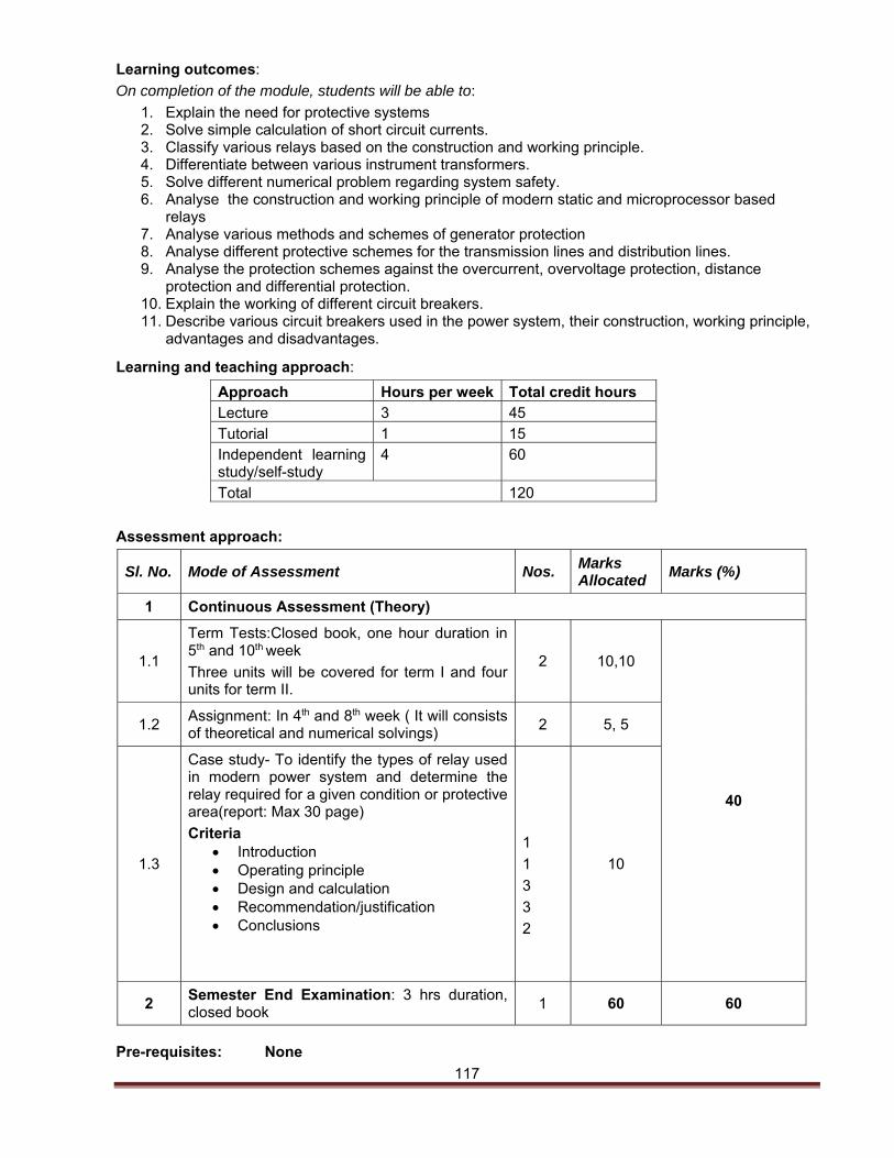
117
Learning outcomes:
On completion of the module, students will be able to:
1. Explain the need for protective systems 2. Solve simple calculation of short circuit currents. 3. Classify various relays based on the construction and working principle. 4. Differentiate between various instrument transformers. 5. Solve different numerical problem regarding system safety. 6. Analyse the construction and working principle of modern static and microprocessor based
relays 7. Analyse various methods and schemes of generator protection 8. Analyse different protective schemes for the transmission lines and distribution lines. 9. Analyse the protection schemes against the overcurrent, overvoltage protection, distance
protection and differential protection. 10. Explain the working of different circuit breakers. 11. Describe various circuit breakers used in the power system, their construction, working principle,
advantages and disadvantages.
Learning and teaching approach:
Approach Hours per week Total credit hours Lecture 3 45 Tutorial 1 15 Independent learning study/self-study
4 60
Total 120
Assessment approach:
Pre-requisites: None
Sl. No. Mode of Assessment Nos. Marks Allocated
Marks (%)
1 Continuous Assessment (Theory)
1.1
Term Tests:Closed book, one hour duration in 5th and 10th week
Three units will be covered for term I and four units for term II.
2 10,10
40
1.2 Assignment: In 4th and 8th week ( It will consists of theoretical and numerical solvings)
2 5, 5
1.3
Case study- To identify the types of relay used in modern power system and determine the relay required for a given condition or protective area(report: Max 30 page)
Criteria Introduction Operating principle Design and calculation Recommendation/justification Conclusions
1
1
3
3
2
10
2 Semester End Examination: 3 hrs duration, closed book
1 60 60
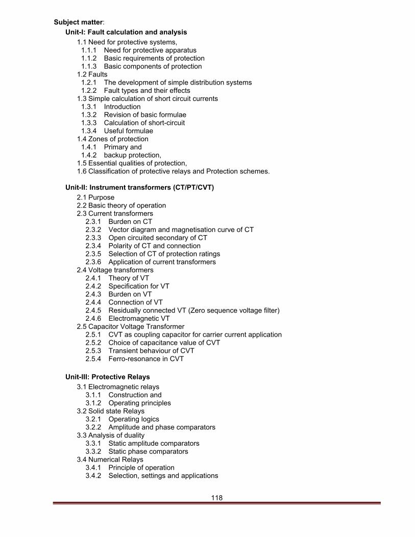
118
Subject matter:
Unit-I: Fault calculation and analysis
1.1 Need for protective systems, 1.1.1 Need for protective apparatus 1.1.2 Basic requirements of protection 1.1.3 Basic components of protection
1.2 Faults 1.2.1 The development of simple distribution systems 1.2.2 Fault types and their effects
1.3 Simple calculation of short circuit currents 1.3.1 Introduction 1.3.2 Revision of basic formulae 1.3.3 Calculation of short-circuit 1.3.4 Useful formulae
1.4 Zones of protection 1.4.1 Primary and 1.4.2 backup protection,
1.5 Essential qualities of protection, 1.6 Classification of protective relays and Protection schemes.
Unit-II: Instrument transformers (CT/PT/CVT)
2.1 Purpose 2.2 Basic theory of operation 2.3 Current transformers
2.3.1 Burden on CT 2.3.2 Vector diagram and magnetisation curve of CT 2.3.3 Open circuited secondary of CT 2.3.4 Polarity of CT and connection 2.3.5 Selection of CT of protection ratings 2.3.6 Application of current transformers
2.4 Voltage transformers 2.4.1 Theory of VT 2.4.2 Specification for VT 2.4.3 Burden on VT 2.4.4 Connection of VT 2.4.5 Residually connected VT (Zero sequence voltage filter) 2.4.6 Electromagnetic VT
2.5 Capacitor Voltage Transformer 2.5.1 CVT as coupling capacitor for carrier current application 2.5.2 Choice of capacitance value of CVT 2.5.3 Transient behaviour of CVT 2.5.4 Ferro-resonance in CVT
Unit-III: Protective Relays
3.1 Electromagnetic relays 3.1.1 Construction and 3.1.2 Operating principles
3.2 Solid state Relays 3.2.1 Operating logics 3.2.2 Amplitude and phase comparators
3.3 Analysis of duality 3.3.1 Static amplitude comparators 3.3.2 Static phase comparators
3.4 Numerical Relays 3.4.1 Principle of operation 3.4.2 Selection, settings and applications
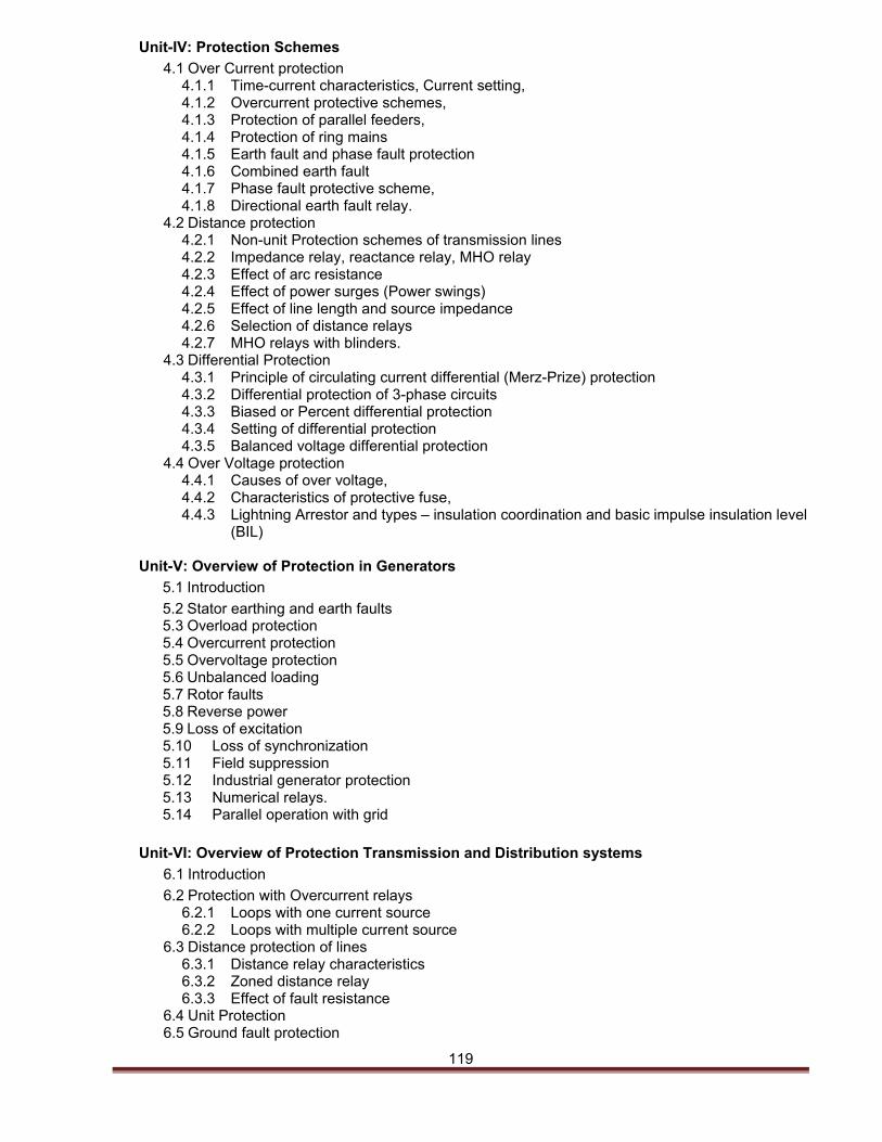
119
Unit-IV: Protection Schemes
4.1 Over Current protection 4.1.1 Time-current characteristics, Current setting, 4.1.2 Overcurrent protective schemes, 4.1.3 Protection of parallel feeders, 4.1.4 Protection of ring mains 4.1.5 Earth fault and phase fault protection 4.1.6 Combined earth fault 4.1.7 Phase fault protective scheme, 4.1.8 Directional earth fault relay.
4.2 Distance protection 4.2.1 Non-unit Protection schemes of transmission lines 4.2.2 Impedance relay, reactance relay, MHO relay 4.2.3 Effect of arc resistance 4.2.4 Effect of power surges (Power swings) 4.2.5 Effect of line length and source impedance 4.2.6 Selection of distance relays 4.2.7 MHO relays with blinders.
4.3 Differential Protection 4.3.1 Principle of circulating current differential (Merz-Prize) protection 4.3.2 Differential protection of 3-phase circuits 4.3.3 Biased or Percent differential protection 4.3.4 Setting of differential protection 4.3.5 Balanced voltage differential protection
4.4 Over Voltage protection 4.4.1 Causes of over voltage, 4.4.2 Characteristics of protective fuse, 4.4.3 Lightning Arrestor and types – insulation coordination and basic impulse insulation level
(BIL)
Unit-V: Overview of Protection in Generators
5.1 Introduction
5.2 Stator earthing and earth faults 5.3 Overload protection 5.4 Overcurrent protection 5.5 Overvoltage protection 5.6 Unbalanced loading 5.7 Rotor faults 5.8 Reverse power 5.9 Loss of excitation 5.10 Loss of synchronization 5.11 Field suppression 5.12 Industrial generator protection 5.13 Numerical relays. 5.14 Parallel operation with grid
Unit-VI: Overview of Protection Transmission and Distribution systems
6.1 Introduction
6.2 Protection with Overcurrent relays 6.2.1 Loops with one current source 6.2.2 Loops with multiple current source
6.3 Distance protection of lines 6.3.1 Distance relay characteristics 6.3.2 Zoned distance relay 6.3.3 Effect of fault resistance
6.4 Unit Protection 6.5 Ground fault protection
120
6.5.1 Importance of ground fault protection 6.5.2 Unique characteristics of ground fault 6.5.3 Polarization of ground relays 6.5.4 Types of ground relays
Unit-VII: Circuit Breakers
7.1 Arc-Extinction
7.1.1 Arc voltage 7.1.2 Arc interruption 7.1.3 Re-striking voltage 7.1.4 Recovery voltage
7.2 Resistance switching 7.3 Current chopping 7.4 Classification of circuit breakers
7.4.1 SF6 CB 7.4.2 Vacuum CB 7.4.3 Operating mechanism
7.5 Selection of circuit breakers 7.6 High voltage DC circuit breakers 7.7 Testing of circuit breakers.
Reading List:
Essential reading
1. Rao, S. S., (2003). Switchgear Protection and Power Systems. New Delhi: Khanna Publishers.
2. Ravindranath & Chander (1995). Power System Protection and Switchgear. New Delhi: New Age International.
3. Mason, C.R., (2008). Art and Science of Protective Relaying, (3 ed.). New Delhi: John Willey.
4. BadriRam & Vishwakarma, D.N. (1995). Power System Protection and Switchgear. New Delhi: TMH PublishingCompany Ltd.
Additional reading
1. Wadhwa, C.L., (2003). Electrical Power Systems. New Delhi: Wiley Eastern Ltd. New Age International.
2. Van A.R., & Warrington, C. (1997). Protective Relays Theory and Practice (Vol.I and II). New Delhi: Chapman and Hall.
3. Kimbark, E.W., (2011). Power System Stability (Vol. II). New Delhi: John Wiulley and Sons, Inc.
4. MadhavaRao, T.S., (2010). Power System Protection; Static Relays. New Delhi: Tata McGraw Hill Publishing Co. Ltd.
Module Code and Title: COM401Communication Engineering Programme : BE in Electrical Engineering Credit : 12 Module Tutor : Chencho General Objectives: This module will familiarize students with the concept of Communication Engineering and types of communication system. Students will be able to understand how information can be transmitted over the channel and methods to measure information. Learning Outcomes: On completion of the module, students will be able to:
1. Perform basic signal operations on analog signals 2. Compute frequency spectrum for real time signals 3. Analyze the analogue signals in time domain and frequency domain 4. Identify the basic elements of communication systems 5. Differentiate mathematically between AM, FM and PM
121
6. Differentiate mathematically between ASK, BFSK , BPSK, QPSK and QAM 7. Describe multiplexing (TDM and FDM). 8. Use different methods to calculate information 9. Measure Characteristics impedance for balanced and un-balanced transmission lines 10. Define the fundamentals of Antennas and electromagnetic radiations.
Learning and Teaching Approach:
Approach Hours per Week Total Credit Hours
Lecture 3 45
Practical 2 30
Independent study/self-directed learning 3 45
Total 120
Assessment Approach:
Sl. No. Mode of Assessment Nos. Marks Allocated Marks (%)
1 Continuous Assessment (Theory)
1.1 Term Test: closed book, one hour duration in 5th (Unit-I and II) and 10th week (Unit-III & IV)
2 20 25
1.2
Assignment: 1assignment each at the end of 2nd and 4th unit.
2 5
Assignment 1: Problem solving to be able to differentiate between AM, PM, FM
1 2.5
Assignment 2: Group work to demonstrate observations using the matlab simulation model to be able to mathematically model communication systems
1 2.5
2 Practical
2.1
Lab report, weekly Assessments (Aims, procedure, circuit diagrams, observations, conclusion). The reports will also be assessed for neatness and representation of data. (10 marks each for every lab conducted. This is averaged over 10 labs and converted to out of 15)
10 15
25
2.2 Practical Exam 1 5
2.3 Viva-Voce 1 5
3 Semester Examination: 3 hrs duration, closed book
1 50 50
Pre-requisites: None
Subject Matter:
Unit I: Concept of Modulation and Demodulation
1.1 Elements of communication 1.1.1 Functional block diagram of communication systems 1.1.2 types of signals, analog and digital 1.1.3 spectrum of signals
122
1.1.4 Time and Frequency domain representation of signals 1.1.5 Telecommunication services and transmission medium
1.2 Amplitude modulation (AM) 1.2.1 Double sideband (DSB) 1.2.2 double sideband suppressed carrier (DSBSC); 1.2.3 single sideband suppressed carrier (SSBSC) 1.2.4 vestigial sideband (VSB) modulation,
1.3 Angle modulation - phase modulation (PM) & 1.3.1 Frequency modulation (FM) 1.3.2 Narrow and wideband FM. 1.3.3 Representation of narrowband noise; receiver model 1.3.4 Signal to noise ratio (SNR), noise figure, noise temperature 1.3.5 Noise in DSB-SC and SSB 1.3.6 AM & FM receivers, pre-emphasis and de-emphasis.
1.4 Pulse Code Modulation 1.4.1 Sampling theorem; Nyquist criteria 1.4.2 pulse amplitude modulation (PAM), pulse width modulation
(PWM), pulse position modulation (PPM) 1.5 Multiplexing
1.5.1 Frequency division multiplexing 1.5.2 Time division multiplexing
Unit II : Power Line Carrier Communication 2.1 Introduction-Main components of PLCC 2.1.1 Transmitters and Receivers, Hybrids and Filters, Line Matching Unit,
Wave Traps, Power Amplifier 2.2 General line equations –loading, reflection and standing waves 2.3 Impedance matching in lines; Stubs, Smith Chart 2.4 Application of PLC in carrier protection relaying- phase and angle
comparison. Unit III : Optical Fiber Communication 3.1 Principles and systems 3.2 Time-Domain method & Frequency Domain Method, 3.3 Geometrical Measurements
3.3.1 diameter, deformation, eccentricity, ellipticity, 3.3.2 Mechanical Strength of Optical Fiber.
3.4 Transmitters and Receivers 3.4.1 Transmission Characteristics of fibers, 3.4.2 short haul and long haul and 3.4.3 high speed links 3.4.4 optical power budget calculations
3.5 Optical Interconnecting Devices: 3.5.1 Optical isolators 3.5.2 polarizer, circulators, attenuators, amplifiers, oscillators, filters 3.5.3 add/drop multiplexers, optical modulators,
Unit IV: Satellite Communication 4.1 GEO Satellite Communication
4.1.1 GEO satellite systems and Orbit calculation,
4.1.2 Two hop and multi hop communication
4.2 Earth Station : The Antenna, High power amplifier, Low noise amplifier, VP connector, Down converters, conversion process, redundancy configuration,
4.3 Satellite transponder design, Transponder model,
123
4.4 Synchronous satellite communication relay by synchronous satellite
Reading List:
Essential Reading:
1. Haykins, S. (2004). An Introduction to Analog and Digital Communication systems. (4ed.). Singapore: John Wiley &Sons.
2. Couch II, W. L. (2004). Digital and Analog Communication System (6ed.). New Delhi: Pearson Education.
3. Couch, W.L., 2004. Modern Communication Systems: Principle and applications (2ed.). New Delhi: Prentice Hall.
Additional Reading:
1. Carlson,B.A. (2002).Communication Systems: An introduction to Signal and noise in Electrical communication (4ed.). New Delhi: McGraw Hill.
2. Kennedy, G. & Davis, B. (2003). Electronic Communication Systems (4ed.).New Delhi: Tata McGraw Hill.
3. Tomasi, W. (2008). Electronic Communication System: Fundamental through Advanced, (5ed.). New Delhi: Pearson Education.
4. Lathi, B. P. & Ding, Z. (2011). Modern Analog and Digital Communication (4ed.). Singapore: John Wiley & Sons.
5. Simon, H. & Moher, M. (2009). Communication Systems (5ed.). Wiley. 6. Taub & Schilling., (1998). Principles of Communication Systems (4ed.). New Delhi: Tata McGraw
Hill. 7. Liao, S.Y., (2003). Microwave Devices and Circuits (5ed.). New Delhi: PHI Private Limited.
Date: January 28, 2017
Module Code and Title : SNP201 Signals and Systems Programme : BE in Electronics and Communication Engineering Credit : 12 Module Tutor(s) : Ms.Dechen Lhamo
General objectives:
This module will enable the students to understand different types of signals encountered in communication engineering, to study their behaviour in time and frequency domain, to make students familiar about Fourier transform for the purpose of signal analysis, to use appropriate tools for signal and system analysis, to understand about noise and their rejection by electronic filters required in communication engineering,
Learning outcomes:
On completion of the module, students will be able to:
1. Distinguish the different types of signals. 2. Analyse LTI system (differential and difference equations). 3. Utilize Fourier Transform & software tools to analyse signals by Fourier Transform. 4. Utilize Z Transform to analyse signals by Z Transform. 5. Judge about types & sources of noise. 6. Construct, design & develop different filters to reject noise. 7. Analyse random signals and Process. 8. Simulate the signals using appropriate tools
Learning and teaching approach:
Approach Hours per Week Total Credit Hours
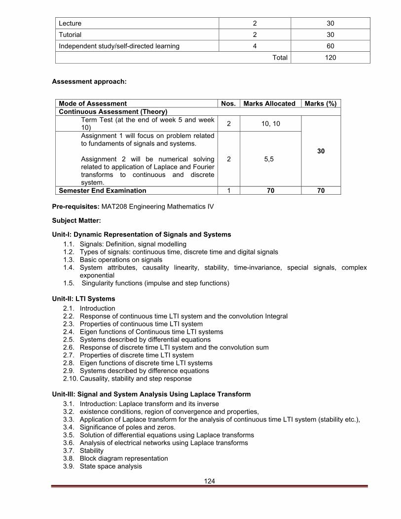
124
Lecture 2 30
Tutorial 2 30
Independent study/self-directed learning 4 60
Total 120
Assessment approach:
Mode of Assessment Nos. Marks Allocated Marks (%) Continuous Assessment (Theory)
Term Test (at the end of week 5 and week 10)
2 10, 10
30
Assignment 1 will focus on problem related to fundaments of signals and systems. Assignment 2 will be numerical solving related to application of Laplace and Fourier transforms to continuous and discrete system.
2 5,5
Semester End Examination 1 70 70 Pre-requisites: MAT208 Engineering Mathematics IV
Subject Matter:
Unit-I: Dynamic Representation of Signals and Systems
1.1. Signals: Definition, signal modelling 1.2. Types of signals: continuous time, discrete time and digital signals 1.3. Basic operations on signals 1.4. System attributes, causality linearity, stability, time-invariance, special signals, complex
exponential 1.5. Singularity functions (impulse and step functions)
Unit-II: LTI Systems
2.1. Introduction 2.2. Response of continuous time LTI system and the convolution Integral 2.3. Properties of continuous time LTI system 2.4. Eigen functions of Continuous time LTI systems 2.5. Systems described by differential equations 2.6. Response of discrete time LTI system and the convolution sum 2.7. Properties of discrete time LTI system 2.8. Eigen functions of discrete time LTI systems 2.9. Systems described by difference equations 2.10. Causality, stability and step response
Unit-III: Signal and System Analysis Using Laplace Transform
3.1. Introduction: Laplace transform and its inverse 3.2. existence conditions, region of convergence and properties, 3.3. Application of Laplace transform for the analysis of continuous time LTI system (stability etc.), 3.4. Significance of poles and zeros. 3.5. Solution of differential equations using Laplace transforms 3.6. Analysis of electrical networks using Laplace transforms 3.7. Stability 3.8. Block diagram representation 3.9. State space analysis
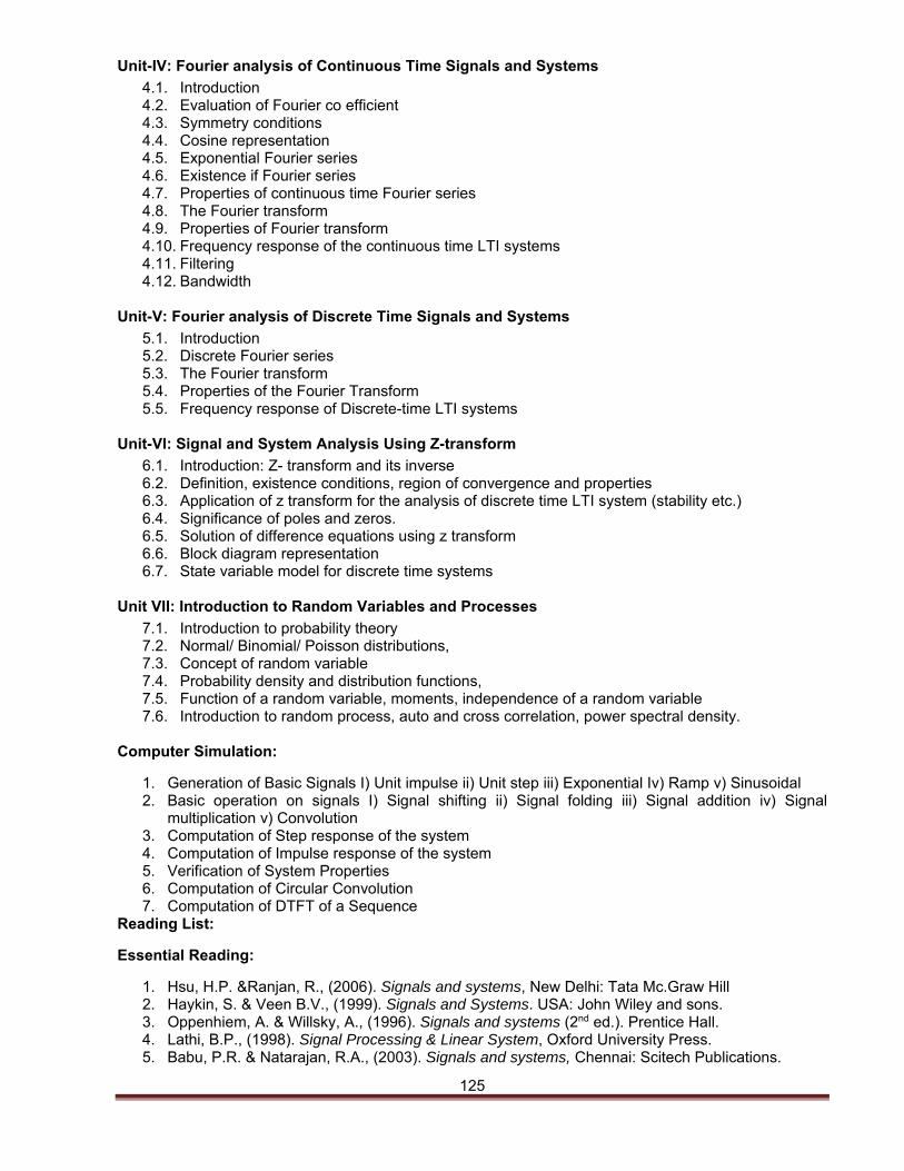
125
Unit-IV: Fourier analysis of Continuous Time Signals and Systems
4.1. Introduction 4.2. Evaluation of Fourier co efficient 4.3. Symmetry conditions 4.4. Cosine representation 4.5. Exponential Fourier series 4.6. Existence if Fourier series 4.7. Properties of continuous time Fourier series 4.8. The Fourier transform 4.9. Properties of Fourier transform 4.10. Frequency response of the continuous time LTI systems 4.11. Filtering 4.12. Bandwidth
Unit-V: Fourier analysis of Discrete Time Signals and Systems
5.1. Introduction 5.2. Discrete Fourier series 5.3. The Fourier transform 5.4. Properties of the Fourier Transform 5.5. Frequency response of Discrete-time LTI systems
Unit-VI: Signal and System Analysis Using Z-transform
6.1. Introduction: Z- transform and its inverse 6.2. Definition, existence conditions, region of convergence and properties 6.3. Application of z transform for the analysis of discrete time LTI system (stability etc.) 6.4. Significance of poles and zeros. 6.5. Solution of difference equations using z transform 6.6. Block diagram representation 6.7. State variable model for discrete time systems
Unit VII: Introduction to Random Variables and Processes
7.1. Introduction to probability theory 7.2. Normal/ Binomial/ Poisson distributions, 7.3. Concept of random variable 7.4. Probability density and distribution functions, 7.5. Function of a random variable, moments, independence of a random variable 7.6. Introduction to random process, auto and cross correlation, power spectral density.
Computer Simulation:
1. Generation of Basic Signals I) Unit impulse ii) Unit step iii) Exponential Iv) Ramp v) Sinusoidal 2. Basic operation on signals I) Signal shifting ii) Signal folding iii) Signal addition iv) Signal
multiplication v) Convolution 3. Computation of Step response of the system 4. Computation of Impulse response of the system 5. Verification of System Properties 6. Computation of Circular Convolution 7. Computation of DTFT of a Sequence
Reading List:
Essential Reading:
1. Hsu, H.P. &Ranjan, R., (2006). Signals and systems, New Delhi: Tata Mc.Graw Hill 2. Haykin, S. & Veen B.V., (1999). Signals and Systems. USA: John Wiley and sons. 3. Oppenhiem, A. & Willsky, A., (1996). Signals and systems (2nd ed.). Prentice Hall. 4. Lathi, B.P., (1998). Signal Processing & Linear System, Oxford University Press. 5. Babu, P.R. & Natarajan, R.A., (2003). Signals and systems, Chennai: Scitech Publications.
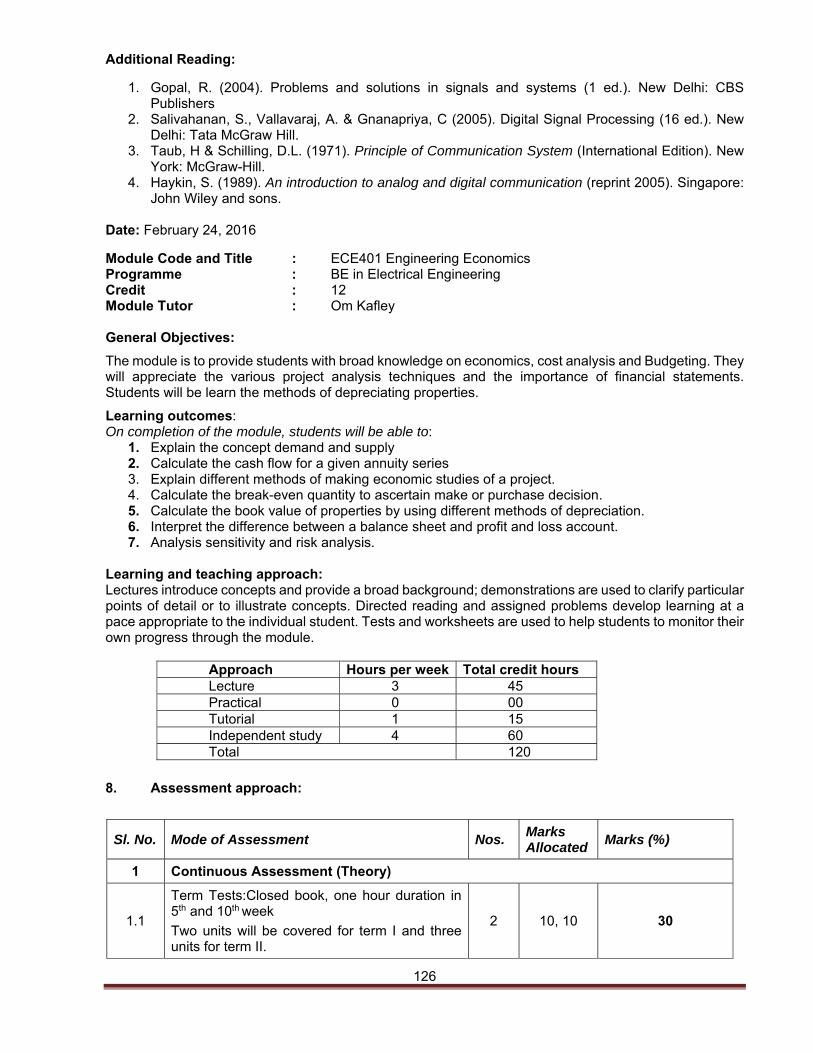
126
Additional Reading:
1. Gopal, R. (2004). Problems and solutions in signals and systems (1 ed.). New Delhi: CBS Publishers
2. Salivahanan, S., Vallavaraj, A. & Gnanapriya, C (2005). Digital Signal Processing (16 ed.). New Delhi: Tata McGraw Hill.
3. Taub, H & Schilling, D.L. (1971). Principle of Communication System (International Edition). New York: McGraw-Hill.
4. Haykin, S. (1989). An introduction to analog and digital communication (reprint 2005). Singapore: John Wiley and sons.
Date: February 24, 2016
Module Code and Title : ECE401 Engineering Economics Programme : BE in Electrical Engineering Credit : 12 Module Tutor : Om Kafley General Objectives:
The module is to provide students with broad knowledge on economics, cost analysis and Budgeting. They will appreciate the various project analysis techniques and the importance of financial statements. Students will be learn the methods of depreciating properties.
Learning outcomes: On completion of the module, students will be able to:
1. Explain the concept demand and supply 2. Calculate the cash flow for a given annuity series 3. Explain different methods of making economic studies of a project. 4. Calculate the break-even quantity to ascertain make or purchase decision. 5. Calculate the book value of properties by using different methods of depreciation. 6. Interpret the difference between a balance sheet and profit and loss account. 7. Analysis sensitivity and risk analysis.
Learning and teaching approach: Lectures introduce concepts and provide a broad background; demonstrations are used to clarify particular points of detail or to illustrate concepts. Directed reading and assigned problems develop learning at a pace appropriate to the individual student. Tests and worksheets are used to help students to monitor their own progress through the module.
Approach Hours per week Total credit hours Lecture 3 45 Practical 0 00 Tutorial 1 15 Independent study 4 60 Total 120
8. Assessment approach:
Sl. No. Mode of Assessment Nos. Marks Allocated
Marks (%)
1 Continuous Assessment (Theory)
1.1
Term Tests:Closed book, one hour duration in 5th and 10th week
Two units will be covered for term I and three units for term II.
2 10, 10 30
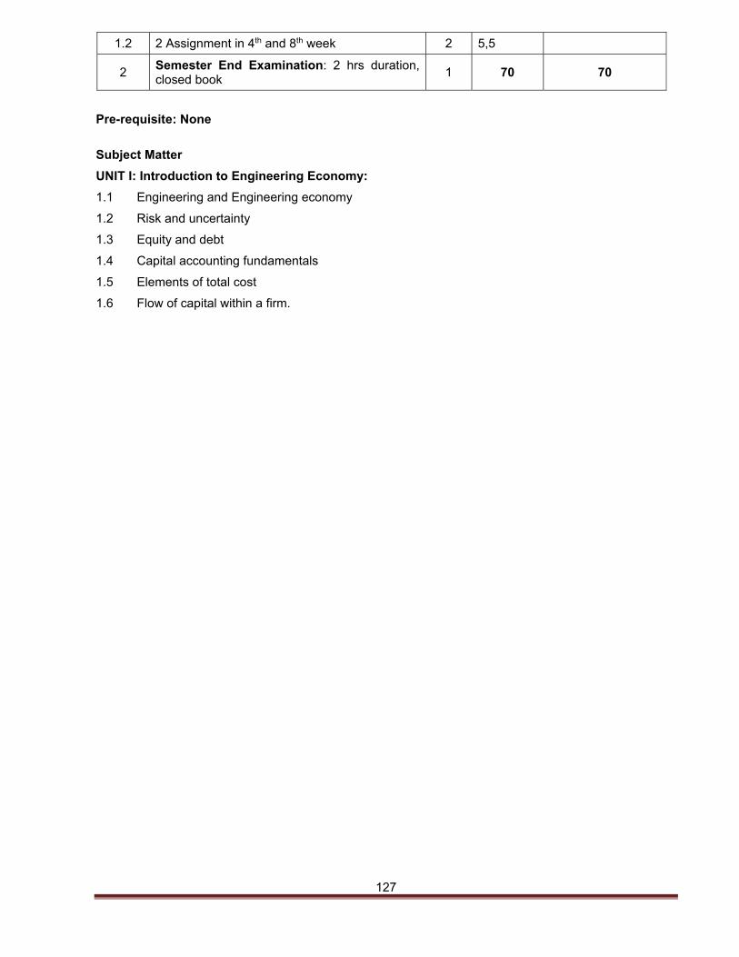
127
Pre-requisite: None
Subject Matter
UNIT I: Introduction to Engineering Economy:
1.1 Engineering and Engineering economy
1.2 Risk and uncertainty
1.3 Equity and debt
1.4 Capital accounting fundamentals
1.5 Elements of total cost
1.6 Flow of capital within a firm.
1.2 2 Assignment in 4th and 8th week 2 5,5
2 Semester End Examination: 2 hrs duration, closed book
1 70 70
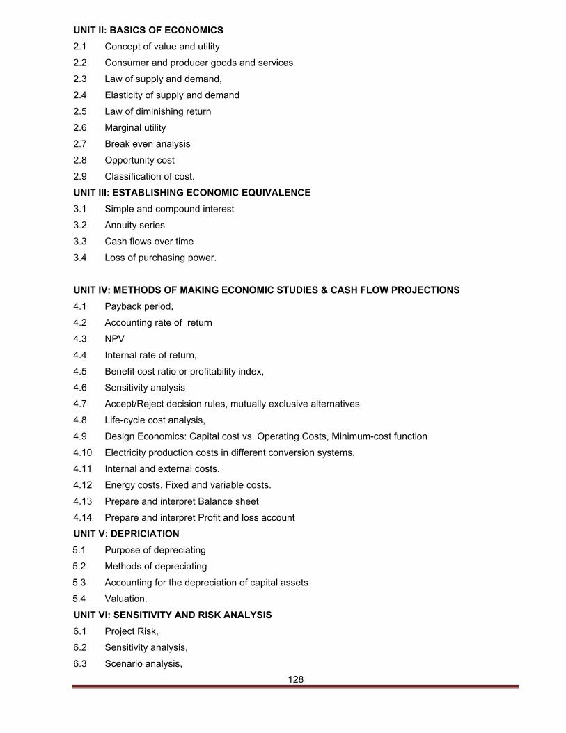
128
UNIT II: BASICS OF ECONOMICS
2.1 Concept of value and utility
2.2 Consumer and producer goods and services
2.3 Law of supply and demand,
2.4 Elasticity of supply and demand
2.5 Law of diminishing return
2.6 Marginal utility
2.7 Break even analysis
2.8 Opportunity cost
2.9 Classification of cost.
UNIT III: ESTABLISHING ECONOMIC EQUIVALENCE
3.1 Simple and compound interest
3.2 Annuity series
3.3 Cash flows over time
3.4 Loss of purchasing power.
UNIT IV: METHODS OF MAKING ECONOMIC STUDIES & CASH FLOW PROJECTIONS
4.1 Payback period,
4.2 Accounting rate of return
4.3 NPV
4.4 Internal rate of return,
4.5 Benefit cost ratio or profitability index,
4.6 Sensitivity analysis
4.7 Accept/Reject decision rules, mutually exclusive alternatives
4.8 Life-cycle cost analysis,
4.9 Design Economics: Capital cost vs. Operating Costs, Minimum-cost function
4.10 Electricity production costs in different conversion systems,
4.11 Internal and external costs.
4.12 Energy costs, Fixed and variable costs.
4.13 Prepare and interpret Balance sheet
4.14 Prepare and interpret Profit and loss account
UNIT V: DEPRICIATION
5.1 Purpose of depreciating
5.2 Methods of depreciating
5.3 Accounting for the depreciation of capital assets
5.4 Valuation.
UNIT VI: SENSITIVITY AND RISK ANALYSIS
6.1 Project Risk,
6.2 Sensitivity analysis,
6.3 Scenario analysis,
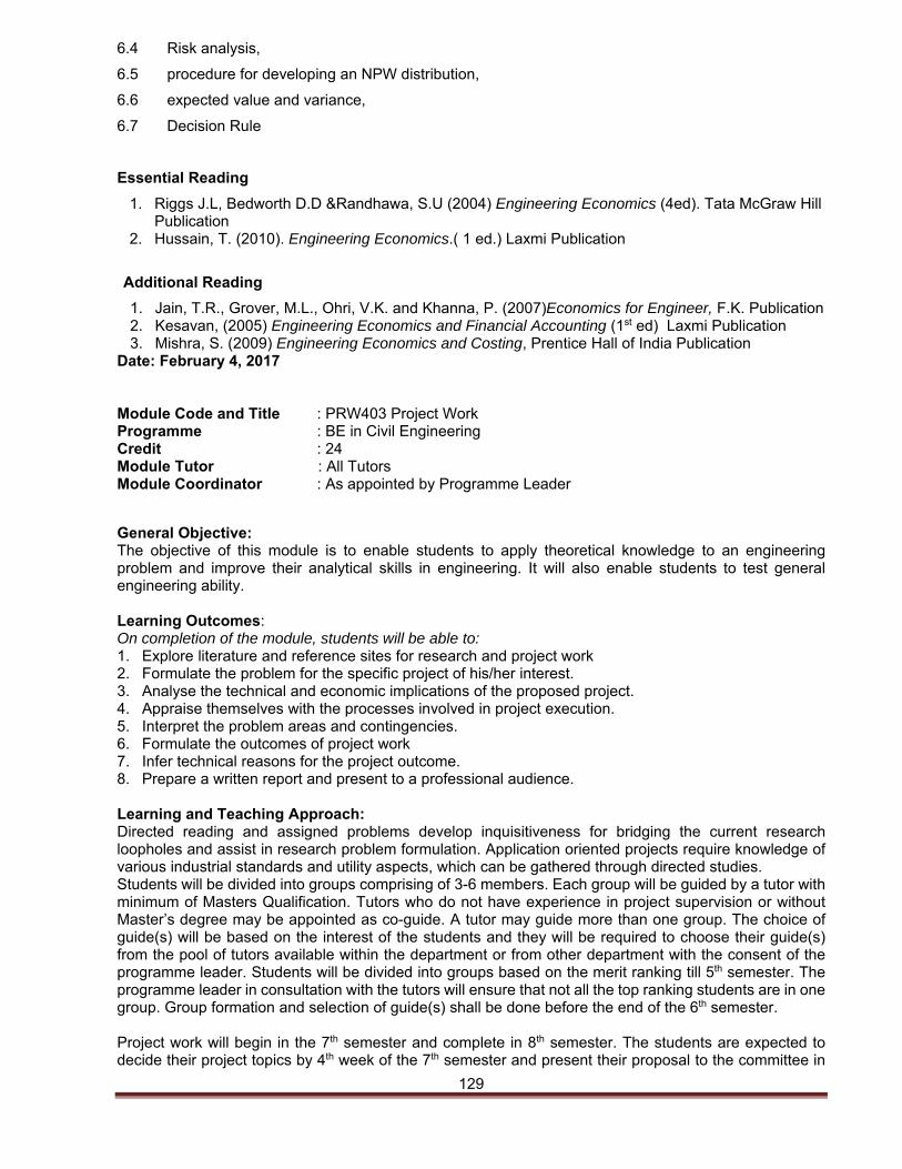
129
6.4 Risk analysis,
6.5 procedure for developing an NPW distribution,
6.6 expected value and variance,
6.7 Decision Rule
Essential Reading
1. Riggs J.L, Bedworth D.D &Randhawa, S.U (2004) Engineering Economics (4ed). Tata McGraw Hill Publication
2. Hussain, T. (2010). Engineering Economics.( 1 ed.) Laxmi Publication
Additional Reading
1. Jain, T.R., Grover, M.L., Ohri, V.K. and Khanna, P. (2007)Economics for Engineer, F.K. Publication 2. Kesavan, (2005) Engineering Economics and Financial Accounting (1st ed) Laxmi Publication 3. Mishra, S. (2009) Engineering Economics and Costing, Prentice Hall of India Publication
Date: February 4, 2017 Module Code and Title : PRW403 Project Work Programme : BE in Civil Engineering Credit : 24 Module Tutor : All Tutors Module Coordinator : As appointed by Programme Leader
General Objective: The objective of this module is to enable students to apply theoretical knowledge to an engineering problem and improve their analytical skills in engineering. It will also enable students to test general engineering ability. Learning Outcomes: On completion of the module, students will be able to: 1. Explore literature and reference sites for research and project work 2. Formulate the problem for the specific project of his/her interest. 3. Analyse the technical and economic implications of the proposed project. 4. Appraise themselves with the processes involved in project execution. 5. Interpret the problem areas and contingencies. 6. Formulate the outcomes of project work 7. Infer technical reasons for the project outcome. 8. Prepare a written report and present to a professional audience. Learning and Teaching Approach: Directed reading and assigned problems develop inquisitiveness for bridging the current research loopholes and assist in research problem formulation. Application oriented projects require knowledge of various industrial standards and utility aspects, which can be gathered through directed studies. Students will be divided into groups comprising of 3-6 members. Each group will be guided by a tutor with minimum of Masters Qualification. Tutors who do not have experience in project supervision or without Master’s degree may be appointed as co-guide. A tutor may guide more than one group. The choice of guide(s) will be based on the interest of the students and they will be required to choose their guide(s) from the pool of tutors available within the department or from other department with the consent of the programme leader. Students will be divided into groups based on the merit ranking till 5th semester. The programme leader in consultation with the tutors will ensure that not all the top ranking students are in one group. Group formation and selection of guide(s) shall be done before the end of the 6th semester. Project work will begin in the 7th semester and complete in 8th semester. The students are expected to decide their project topics by 4th week of the 7th semester and present their proposal to the committee in
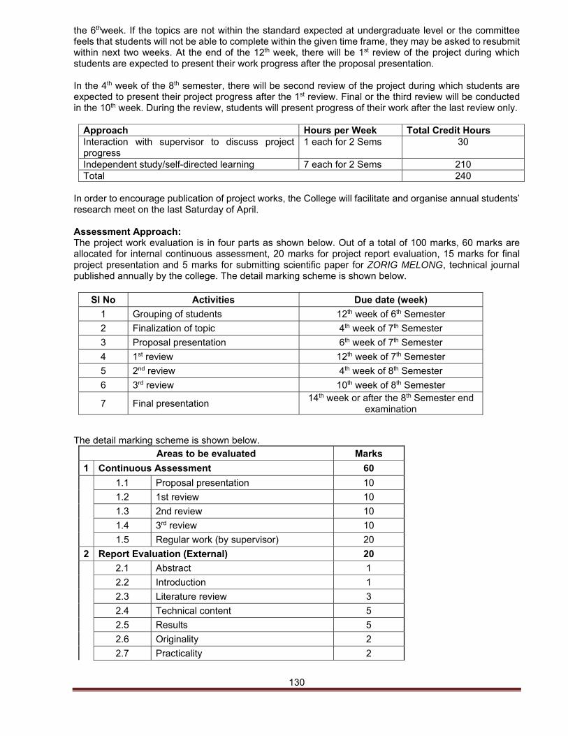
130
the 6thweek. If the topics are not within the standard expected at undergraduate level or the committee feels that students will not be able to complete within the given time frame, they may be asked to resubmit within next two weeks. At the end of the 12th week, there will be 1st review of the project during which students are expected to present their work progress after the proposal presentation. In the 4th week of the 8th semester, there will be second review of the project during which students are expected to present their project progress after the 1st review. Final or the third review will be conducted in the 10th week. During the review, students will present progress of their work after the last review only.
Approach Hours per Week Total Credit Hours Interaction with supervisor to discuss project progress
1 each for 2 Sems 30
Independent study/self-directed learning 7 each for 2 Sems 210 Total 240
In order to encourage publication of project works, the College will facilitate and organise annual students’ research meet on the last Saturday of April. Assessment Approach: The project work evaluation is in four parts as shown below. Out of a total of 100 marks, 60 marks are allocated for internal continuous assessment, 20 marks for project report evaluation, 15 marks for final project presentation and 5 marks for submitting scientific paper for ZORIG MELONG, technical journal published annually by the college. The detail marking scheme is shown below.
Sl No Activities Due date (week)
1 Grouping of students 12th week of 6th Semester
2 Finalization of topic 4th week of 7th Semester
3 Proposal presentation 6th week of 7th Semester
4 1st review 12th week of 7th Semester
5 2nd review 4th week of 8th Semester
6 3rd review 10th week of 8th Semester
7 Final presentation 14th week or after the 8th Semester end
examination
The detail marking scheme is shown below. Areas to be evaluated Marks
1 Continuous Assessment 60
1.1 Proposal presentation 10
1.2 1st review 10
1.3 2nd review 10
1.4 3rd review 10
1.5 Regular work (by supervisor) 20
2 Report Evaluation (External) 20
2.1 Abstract 1
2.2 Introduction 1
2.3 Literature review 3
2.4 Technical content 5
2.5 Results 5
2.6 Originality 2
2.7 Practicality 2
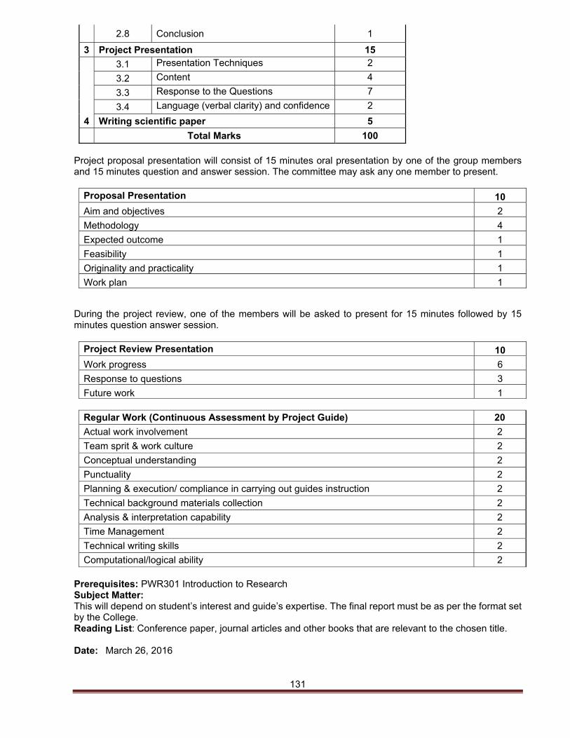
131
2.8 Conclusion 1
3 Project Presentation 15
3.1 Presentation Techniques 2
3.2 Content 4
3.3 Response to the Questions 7
3.4 Language (verbal clarity) and confidence 2
4 Writing scientific paper 5
Total Marks 100
Project proposal presentation will consist of 15 minutes oral presentation by one of the group members and 15 minutes question and answer session. The committee may ask any one member to present.
Proposal Presentation 10
Aim and objectives 2
Methodology 4
Expected outcome 1
Feasibility 1
Originality and practicality 1
Work plan 1
During the project review, one of the members will be asked to present for 15 minutes followed by 15 minutes question answer session.
Project Review Presentation 10
Work progress 6
Response to questions 3
Future work 1
Regular Work (Continuous Assessment by Project Guide) 20
Actual work involvement 2
Team sprit & work culture 2
Conceptual understanding 2
Punctuality 2
Planning & execution/ compliance in carrying out guides instruction 2
Technical background materials collection 2
Analysis & interpretation capability 2
Time Management 2
Technical writing skills 2
Computational/logical ability 2 Prerequisites: PWR301 Introduction to Research Subject Matter: This will depend on student’s interest and guide’s expertise. The final report must be as per the format set by the College. Reading List: Conference paper, journal articles and other books that are relevant to the chosen title. Date: March 26, 2016
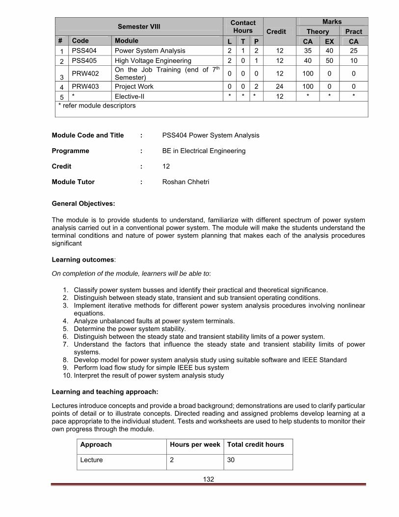
132
Semester VIII Contact Hours Credit
Marks
Theory Pract # Code Module L T P CA EX CA
1 PSS404 Power System Analysis 2 1 2 12 35 40 25
2 PSS405 High Voltage Engineering 2 0 1 12 40 50 10
3 PRW402
On the Job Training (end of 7th Semester)
0 0 0 12 100 0 0
4 PRW403 Project Work 0 0 2 24 100 0 0
5 * Elective-II * * * 12 * * * * refer module descriptors
Module Code and Title : PSS404 Power System Analysis Programme : BE in Electrical Engineering Credit : 12 Module Tutor : Roshan Chhetri
General Objectives:
The module is to provide students to understand, familiarize with different spectrum of power system analysis carried out in a conventional power system. The module will make the students understand the terminal conditions and nature of power system planning that makes each of the analysis procedures significant
Learning outcomes:
On completion of the module, learners will be able to:
1. Classify power system busses and identify their practical and theoretical significance. 2. Distinguish between steady state, transient and sub transient operating conditions. 3. Implement iterative methods for different power system analysis procedures involving nonlinear
equations. 4. Analyze unbalanced faults at power system terminals. 5. Determine the power system stability. 6. Distinguish between the steady state and transient stability limits of a power system. 7. Understand the factors that influence the steady state and transient stability limits of power
systems. 8. Develop model for power system analysis study using suitable software and IEEE Standard 9. Perform load flow study for simple IEEE bus system 10. Interpret the result of power system analysis study
Learning and teaching approach:
Lectures introduce concepts and provide a broad background; demonstrations are used to clarify particular points of detail or to illustrate concepts. Directed reading and assigned problems develop learning at a pace appropriate to the individual student. Tests and worksheets are used to help students to monitor their own progress through the module.
Approach Hours per week Total credit hours
Lecture 2 30
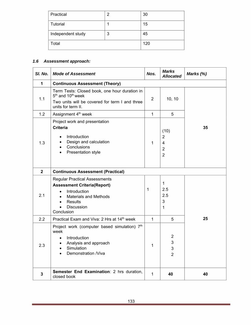
133
Practical 2 30
Tutorial 1 15
Independent study 3 45
Total 120
1.6 Assessment approach:
Sl. No. Mode of Assessment Nos. Marks Allocated
Marks (%)
1 Continuous Assessment (Theory)
1.1
Term Tests: Closed book, one hour duration in 5th and 10th week
Two units will be covered for term I and three units for term II.
2 10, 10
35
1.2 Assignment 4th week 1 5
1.3
Project work and presentation
Criteria
Introduction Design and calculation Conclusions Presentation style
1
(10)
2
4
2
2
2 Continuous Assessment (Practical)
2.1
Regular Practical Assessments
Assessment Criteria(Report)
Introduction Materials and Methods Results Discussion
Conclusion
1
1
2.5
2.5
3
1
25
2.2 Practical Exam and Viva: 2 Hrs at 14th week 1 5
2.3
Project work (computer based simulation) 7th week
Introduction Analysis and approach Simulation Demonstration /Viva
1
2
3
3
2
3 Semester End Examination: 2 hrs duration, closed book
1 40 40
134
Subject matter:
1. UNIT I System Representation: 1.1 Single line representation. 1.2 Per Unit Systems. 1.3 modelling of transformer, load, synchronous machine.
2. UNIT II Formation of Network Matrices: 2.1 Bus admittance and impedance matrices, 2.2 Algorithms for formation of Z-Bus and Y-Bus matrices, 2.3 modification of Z-Bus and Y-Bus matrices. 2.4 Sparsity oriented inversion for Y-Bus.
3. UNIT III Load Flow Studies:
3.1 Bus classification; 3.2 Developing load flow equations; 3.3 Solution techniques – Iterative methods:
3.3.1 Gauss, Gauss-Seidal, 3.3.2 Newton Raphson 3.3.3 Fast-decoupled method;
3.4 Acceleration of convergence; 3.5 Comparison of different methods, merits and demerits.
4. UNIT IV Short Circuit Studies:
4.1 Need of fault studies, types of faults. 4.2 Symmetrical fault Analysis: transient in R- L circuit, doubling effect, selection of circuit breakers
short Circuit Current and MVA Calculations, Fault levels, Application of Series Reactors. 4.3 Symmetrical Component Theory: Symmetrical Component Transformation, Positive, Negative
and Zero sequence components: Voltages, Currents and Impedances. 4.4 Sequence Networks: Positive, Negative and Zero sequence Networks, Numerical Problems. 4.5 Unsymmetrical Fault Analysis: LG, LL, LLG and open conductor faults with and without fault
impedance, numerical Problems. 5. UNIT VI Stability Studies:
5.1 Power System Steady State Stability Analysis, importance of stability analysis for operation, control and design, elementary concepts of steady state, dynamic and transient stabilities. Description of: steady state stability power limit, transfer reactance, synchronizing power coefficient, power angle curve and determination of steady state stability and methods to improve steady state stability.
5.2 Power System Transient State Stability Analysis: Assumption in transient stability studies, derivation of Swing equation, multi-machine stability, determination of transient stability by equal area criterion, application of equal area criterion, and critical clearing angle calculation, solution of swing equation: point-by-point method. Methods to improve stability
5.3 Fault analysis for stability studies. Numerical integration methods, Euler method, modified Euler method, Runge – Kutta methods
5.4 Introduction to voltage stability, effect of excitation system and power system stabilities, development of block diagram and transfer functions
5.5 Basic pricing principles, electricity pricing and markets: market models, demand side management, transmission and distribution pricing, Availability Based tariff (ABT) and unscheduled interchange (UI) mechanism.
5.6 Recent trends to improve stability 6. UNIT VI Introduction to Power System Control:
6.1 Introduction to power system control 6.2 Basic generator control loops 6.3 Load Frequency control 6.4 Generator model, load model, prime mover model, governor model 6.5 Automatic generator control 6.6 Reactive Power and voltage control
6.6.1 Amplifier model 6.6.2 Exciter model 6.6.3 Generator model
135
6.6.4 Sensor model 6.6.5 Excitation system stabilizer
List of Practicals:
1. Develop model for power system analysis using standard IEEE standard bus with 5 to 10 bus 2. Determine the reactive power supply required at bus 2 to maintain 1pu voltage for different
loading condition. 3. Perform load flow studies 4. Perform various short circuit (L-G, L-L-G, L-L, L-L-L ) studies 5. Perform transient studies 6. Perform Shunt and series compensation of transmission lines. 7. Perform reactive power control by a tap changing transformer. 8. Determine the economics of going in for 220 kV single circuit and double circuit.
Reading list
Essential reading
1. Gergen, A.R. (2001), Power system Analysis, Prentice hall Inc. 2. Singh, L.P. (2001), Advanced Power System Analysis and Dynamics, (3 ed), New Age International
Publishers, New Delhi, 3. Nagrath I.J. and Kothari D.P. (2000), Modern Power System Analysis, (2 ed), Tata McGraw Hill,
New Delhi, 4. Stevenson, W.D. (2000), Elements of Power System analysis, (4 ed),Tata McGraw Hill Ltd. 5. Gainger, J. J. and Stevenson Jr, W.D.. (2003), Power System analysis, (1 ed) McGraw Hill. 6. Nagsarkar, T.K. & Sukhija, M.S., (2013), Power System Analysis, (1 ed), Oxford University press,
New Delhi.
Additional reading
1. Kundur, P. (1994), Power System Stability and Control, McGraw Hill Inc. 2. Wadhwa, C. L. (2003), Electrical power System, (3 ed), New Age International Ltd., New Delhi, 3. Gupta, B. R. (2003), Power System Analysis and Design, (3 ed), Wheeler Publishing, New Delhi, 4. Ashtaq, H. (2004), Electrical Power Systems, (4 ed), CBS Publishers and Distributors, New Delhi,
Date: 21st July, 2017
Module Code and Title : PSS405 High Voltage Engineering Programme : BE in Electrical Engineering Credit : 12 Module Tutor : Pravakar Pradhan
General Objectives:
This module will enable students to learn on high-voltage technology and electrical insulating materials. It covers the basic theories and the most important methods of high voltage engineering such as: Generation of high voltages and currents; Non-destructive testing of materials; High voltage test and measurement techniques; Electrical breakdown strength of gaseous, liquid and solid insulators; Dielectric properties of electrical insulation.
Learning outcomes:
On completion of the module, students will be able to:
1. Identify the different applications of high voltage.
2. Analyze basic problems in dealing with high voltage and high currents.
3. Explain theories of breakdown in gaseous, liquid, and solid.
4. Distinguish and explain different types of insulations.
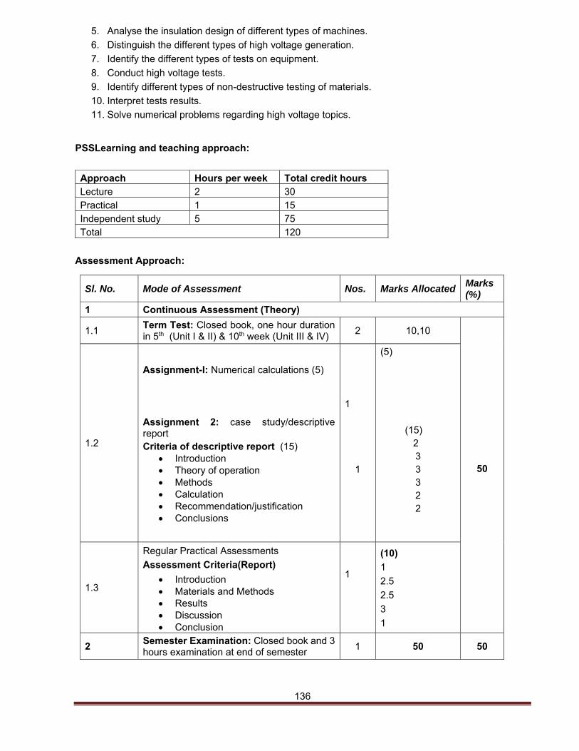
136
5. Analyse the insulation design of different types of machines.
6. Distinguish the different types of high voltage generation.
7. Identify the different types of tests on equipment.
8. Conduct high voltage tests.
9. Identify different types of non-destructive testing of materials.
10. Interpret tests results.
11. Solve numerical problems regarding high voltage topics.
PSSLearning and teaching approach:
Approach Hours per week Total credit hours Lecture 2 30 Practical 1 15 Independent study 5 75 Total 120
Assessment Approach:
Sl. No. Mode of Assessment Nos. Marks Allocated Marks (%)
1 Continuous Assessment (Theory)
1.1 Term Test: Closed book, one hour duration in 5th (Unit I & II) & 10th week (Unit III & IV)
2 10,10
50
1.2
Assignment-I: Numerical calculations (5) Assignment 2: case study/descriptive report Criteria of descriptive report (15)
Introduction Theory of operation Methods Calculation Recommendation/justification Conclusions
1
1
(5) (15) 2
3 3 3 2 2
1.3
Regular Practical Assessments
Assessment Criteria(Report)
Introduction Materials and Methods Results Discussion Conclusion
1
(10)
1
2.5
2.5
3
1
2 Semester Examination: Closed book and 3 hours examination at end of semester
1 50 50
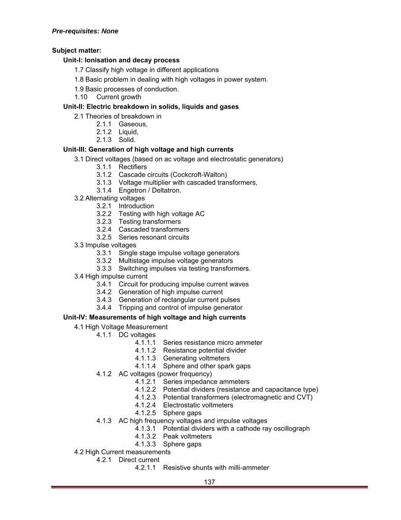
137
Pre-requisites: None
Subject matter:
Unit-I: Ionisation and decay process
1.7 Classify high voltage in different applications
1.8 Basic problem in dealing with high voltages in power system.
1.9 Basic processes of conduction. 1.10 Current growth
Unit-II: Electric breakdown in solids, liquids and gases
2.1 Theories of breakdown in 2.1.1 Gaseous, 2.1.2 Liquid, 2.1.3 Solid.
Unit-III: Generation of high voltage and high currents
3.1 Direct voltages (based on ac voltage and electrostatic generators) 3.1.1 Rectifiers 3.1.2 Cascade circuits (Cockcroft-Walton) 3.1.3 Voltage multiplier with cascaded transformers, 3.1.4 Engetron / Deltatron.
3.2 Alternating voltages 3.2.1 Introduction 3.2.2 Testing with high voltage AC 3.2.3 Testing transformers 3.2.4 Cascaded transformers 3.2.5 Series resonant circuits
3.3 Impulse voltages 3.3.1 Single stage impulse voltage generators 3.3.2 Multistage impulse voltage generators 3.3.3 Switching impulses via testing transformers.
3.4 High impulse current 3.4.1 Circuit for producing impulse current waves 3.4.2 Generation of high impulse current 3.4.3 Generation of rectangular current pulses 3.4.4 Tripping and control of impulse generator
Unit-IV: Measurements of high voltage and high currents
4.1 High Voltage Measurement 4.1.1 DC voltages
4.1.1.1 Series resistance micro ammeter 4.1.1.2 Resistance potential divider 4.1.1.3 Generating voltmeters 4.1.1.4 Sphere and other spark gaps
4.1.2 AC voltages (power frequency) 4.1.2.1 Series impedance ammeters 4.1.2.2 Potential dividers (resistance and capacitance type) 4.1.2.3 Potential transformers (electromagnetic and CVT) 4.1.2.4 Electrostatic voltmeters 4.1.2.5 Sphere gaps
4.1.3 AC high frequency voltages and impulse voltages 4.1.3.1 Potential dividers with a cathode ray oscillograph 4.1.3.2 Peak voltmeters 4.1.3.3 Sphere gaps
4.2 High Current measurements 4.2.1 Direct current
4.2.1.1 Resistive shunts with milli-ammeter
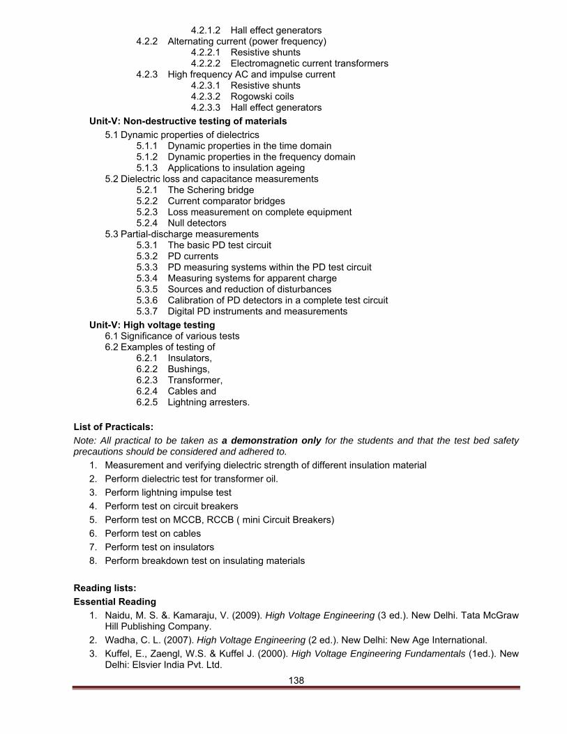
138
4.2.1.2 Hall effect generators 4.2.2 Alternating current (power frequency)
4.2.2.1 Resistive shunts 4.2.2.2 Electromagnetic current transformers
4.2.3 High frequency AC and impulse current 4.2.3.1 Resistive shunts 4.2.3.2 Rogowski coils 4.2.3.3 Hall effect generators
Unit-V: Non-destructive testing of materials
5.1 Dynamic properties of dielectrics 5.1.1 Dynamic properties in the time domain 5.1.2 Dynamic properties in the frequency domain 5.1.3 Applications to insulation ageing
5.2 Dielectric loss and capacitance measurements 5.2.1 The Schering bridge 5.2.2 Current comparator bridges 5.2.3 Loss measurement on complete equipment 5.2.4 Null detectors
5.3 Partial-discharge measurements 5.3.1 The basic PD test circuit 5.3.2 PD currents 5.3.3 PD measuring systems within the PD test circuit 5.3.4 Measuring systems for apparent charge 5.3.5 Sources and reduction of disturbances 5.3.6 Calibration of PD detectors in a complete test circuit 5.3.7 Digital PD instruments and measurements
Unit-V: High voltage testing 6.1 Significance of various tests 6.2 Examples of testing of
6.2.1 Insulators, 6.2.2 Bushings, 6.2.3 Transformer, 6.2.4 Cables and 6.2.5 Lightning arresters.
List of Practicals:
Note: All practical to be taken as a demonstration only for the students and that the test bed safety precautions should be considered and adhered to.
1. Measurement and verifying dielectric strength of different insulation material
2. Perform dielectric test for transformer oil.
3. Perform lightning impulse test
4. Perform test on circuit breakers
5. Perform test on MCCB, RCCB ( mini Circuit Breakers)
6. Perform test on cables
7. Perform test on insulators
8. Perform breakdown test on insulating materials
Reading lists:
Essential Reading
1. Naidu, M. S. &. Kamaraju, V. (2009). High Voltage Engineering (3 ed.). New Delhi. Tata McGraw Hill Publishing Company.
2. Wadha, C. L. (2007). High Voltage Engineering (2 ed.). New Delhi: New Age International.
3. Kuffel, E., Zaengl, W.S. & Kuffel J. (2000). High Voltage Engineering Fundamentals (1ed.). New Delhi: Elsvier India Pvt. Ltd.
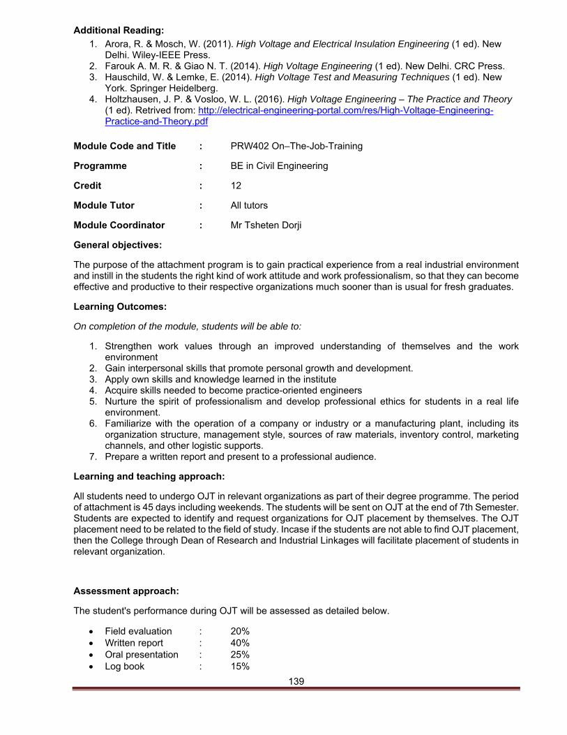
139
Additional Reading:
1. Arora, R. & Mosch, W. (2011). High Voltage and Electrical Insulation Engineering (1 ed). New Delhi. Wiley-IEEE Press.
2. Farouk A. M. R. & Giao N. T. (2014). High Voltage Engineering (1 ed). New Delhi. CRC Press. 3. Hauschild, W. & Lemke, E. (2014). High Voltage Test and Measuring Techniques (1 ed). New
York. Springer Heidelberg. 4. Holtzhausen, J. P. & Vosloo, W. L. (2016). High Voltage Engineering – The Practice and Theory
(1 ed). Retrived from: http://electrical-engineering-portal.com/res/High-Voltage-Engineering-Practice-and-Theory.pdf
Module Code and Title : PRW402 On–The-Job-Training
Programme : BE in Civil Engineering
Credit : 12
Module Tutor : All tutors
Module Coordinator : Mr Tsheten Dorji
General objectives:
The purpose of the attachment program is to gain practical experience from a real industrial environment and instill in the students the right kind of work attitude and work professionalism, so that they can become effective and productive to their respective organizations much sooner than is usual for fresh graduates.
Learning Outcomes:
On completion of the module, students will be able to:
1. Strengthen work values through an improved understanding of themselves and the work environment
2. Gain interpersonal skills that promote personal growth and development. 3. Apply own skills and knowledge learned in the institute 4. Acquire skills needed to become practice-oriented engineers 5. Nurture the spirit of professionalism and develop professional ethics for students in a real life
environment. 6. Familiarize with the operation of a company or industry or a manufacturing plant, including its
organization structure, management style, sources of raw materials, inventory control, marketing channels, and other logistic supports.
7. Prepare a written report and present to a professional audience.
Learning and teaching approach:
All students need to undergo OJT in relevant organizations as part of their degree programme. The period of attachment is 45 days including weekends. The students will be sent on OJT at the end of 7th Semester. Students are expected to identify and request organizations for OJT placement by themselves. The OJT placement need to be related to the field of study. Incase if the students are not able to find OJT placement, then the College through Dean of Research and Industrial Linkages will facilitate placement of students in relevant organization.
Assessment approach:
The student's performance during OJT will be assessed as detailed below.
Field evaluation : 20% Written report : 40% Oral presentation : 25% Log book : 15%
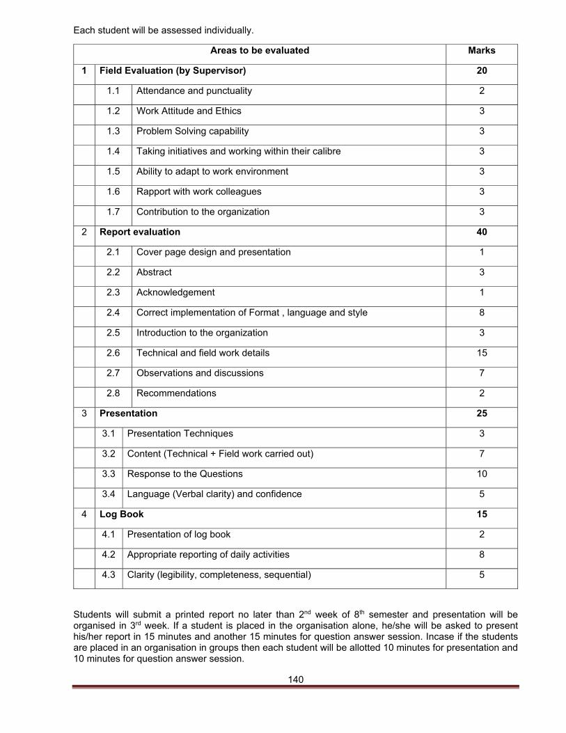
140
Each student will be assessed individually.
Areas to be evaluated Marks
1 Field Evaluation (by Supervisor) 20
1.1 Attendance and punctuality 2
1.2 Work Attitude and Ethics 3
1.3 Problem Solving capability 3
1.4 Taking initiatives and working within their calibre 3
1.5 Ability to adapt to work environment 3
1.6 Rapport with work colleagues 3
1.7 Contribution to the organization 3
2 Report evaluation 40
2.1 Cover page design and presentation 1
2.2 Abstract 3
2.3 Acknowledgement 1
2.4 Correct implementation of Format , language and style 8
2.5 Introduction to the organization 3
2.6 Technical and field work details 15
2.7 Observations and discussions 7
2.8 Recommendations 2
3 Presentation 25
3.1 Presentation Techniques 3
3.2 Content (Technical + Field work carried out) 7
3.3 Response to the Questions 10
3.4 Language (Verbal clarity) and confidence 5
4 Log Book 15
4.1 Presentation of log book 2
4.2 Appropriate reporting of daily activities 8
4.3 Clarity (legibility, completeness, sequential) 5
Students will submit a printed report no later than 2nd week of 8th semester and presentation will be organised in 3rd week. If a student is placed in the organisation alone, he/she will be asked to present his/her report in 15 minutes and another 15 minutes for question answer session. Incase if the students are placed in an organisation in groups then each student will be allotted 10 minutes for presentation and 10 minutes for question answer session.
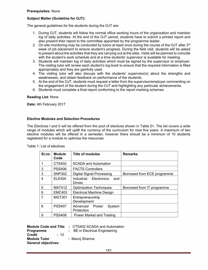
141
Prerequisites: None
Subject Matter (Guideline for OJT):
The general guidelines for the students during the OJT are:
1. During OJT, students will follow the normal office working hours of the organization and maintain log of daily activities. At the end of the OJT period, students have to submit a printed report and also present their report to the committee appointed by the programme leader.
2. On-site monitoring may be conducted by tutors at least once during the course of the OJT after 3rd week of job placement to ensure student’s progress. During the field visit, students will be asked to present about the activities that they are carrying out at the sites. Visits will be planned to coincide with the student’s work schedule and at a time students’ supervisor is available for meeting.
3. Students will maintain log of daily activities which must be signed by the supervisor or employer. The visiting tutor will review each student’s log book to ensure that the required information is filled appropriately and they are gainfully used.
4. The visiting tutor will also discuss with the students’ supervisor(s) about the strengths and weaknesses, and obtain feedback on performance of the students.
5. At the end of the OJT, students must request a letter from the supervisor/employer commenting on the engagement of the student during the OJT and highlighting any particular achievements.
6. Students must complete a final report conforming to the report marking schemes
Reading List: None
Date: 4th February 2017
Elective Modules and Selection Procedures
The Electives I and II will be offered from the pool of electives shown in Table 01. The list covers a wide range of modules which will uplift the currency of the curriculum for next five years. A maximum of two elective modules will be offered in a semester, however there should be a minimum of 10 students registered for a module to optimize the resources.
Table 1: List of electives
Sl.no Module Code
Title of modules Remarks
1 CTS402 SCADA and Automation
3 PSS406 FACTS Controllers 3 SNP302 Digital Signal Processing Borrowed from ECE programme 4 ELE404 Industrial Electronics and
Drives
5 MAT412 Optimization Techniques Borrowed from IT programme 6 EMC403 Electrical Machine Design7 MGT301 Entrepreneurship
Development
8 PSS407 Advanced Power System Protection
9 PSS408 Power Market and Trading
Module Code and Title : CTS402 SCADA and Automation Programme : BE in Electrical Engineering Credit : 12 Module Tutor : Manoj Sharma General objectives:
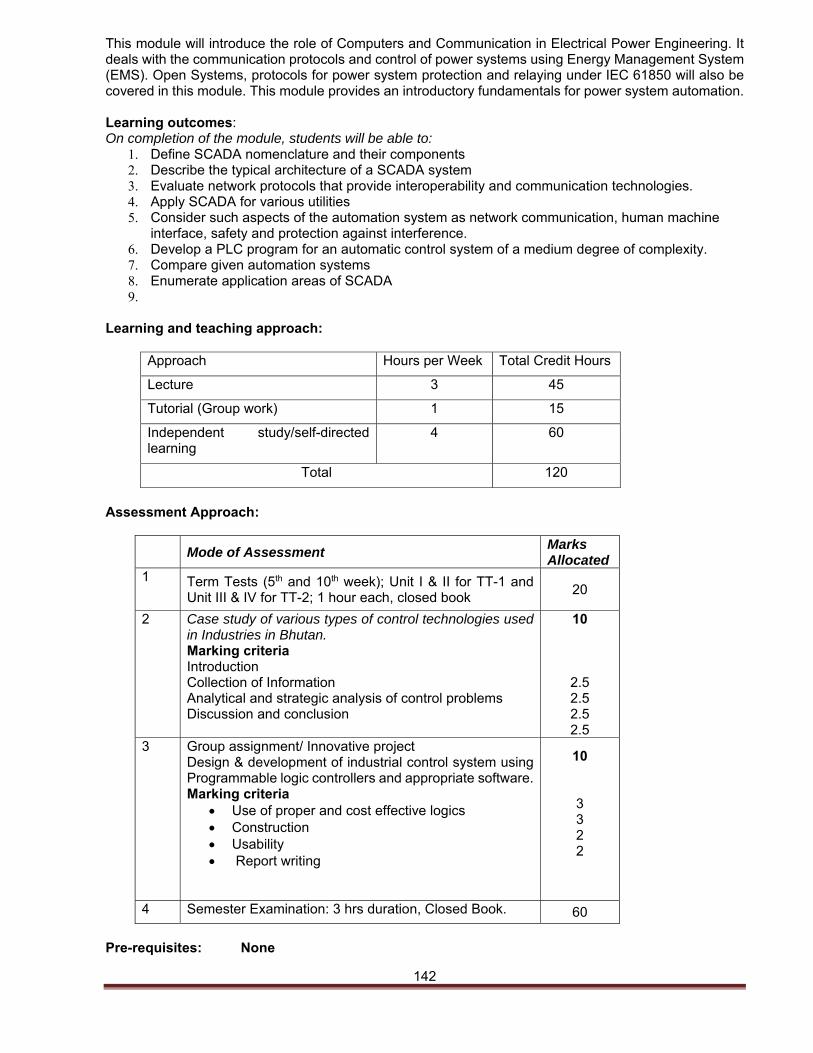
142
This module will introduce the role of Computers and Communication in Electrical Power Engineering. It deals with the communication protocols and control of power systems using Energy Management System (EMS). Open Systems, protocols for power system protection and relaying under IEC 61850 will also be covered in this module. This module provides an introductory fundamentals for power system automation. Learning outcomes: On completion of the module, students will be able to:
1. Define SCADA nomenclature and their components 2. Describe the typical architecture of a SCADA system 3. Evaluate network protocols that provide interoperability and communication technologies. 4. Apply SCADA for various utilities 5. Consider such aspects of the automation system as network communication, human machine
interface, safety and protection against interference. 6. Develop a PLC program for an automatic control system of a medium degree of complexity. 7. Compare given automation systems 8. Enumerate application areas of SCADA 9.
Learning and teaching approach:
Approach Hours per Week Total Credit Hours
Lecture 3 45
Tutorial (Group work) 1 15
Independent study/self-directed learning
4 60
Total 120
Assessment Approach:
Mode of Assessment
Marks Allocated
1 Term Tests (5th and 10th week); Unit I & II for TT-1 and Unit III & IV for TT-2; 1 hour each, closed book
20
2 Case study of various types of control technologies used in Industries in Bhutan. Marking criteria Introduction Collection of Information Analytical and strategic analysis of control problems Discussion and conclusion
10
2.5 2.5 2.5 2.5
3 Group assignment/ Innovative project Design & development of industrial control system using Programmable logic controllers and appropriate software.Marking criteria
Use of proper and cost effective logics Construction Usability Report writing
10
3 3 2 2
4 Semester Examination: 3 hrs duration, Closed Book. 60
Pre-requisites: None
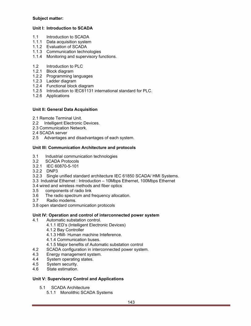
143
Subject matter: Unit I: Introduction to SCADA
1.1 Introduction to SCADA 1.1.1 Data acquisition system 1.1.2 Evaluation of SCADA 1.1.3 Communication technologies 1.1.4 Monitoring and supervisory functions.
1.2 Introduction to PLC 1.2.1 Block diagram 1.2.2 Programming languages 1.2.3 Ladder diagram 1.2.4 Functional block diagram 1.2.5 Introduction to IEC61131 international standard for PLC. 1.2.6 Applications
Unit II: General Data Acquisition
2.1 Remote Terminal Unit. 2.2 Intelligent Electronic Devices. 2.3 Communication Network. 2.4 SCADA server 2.5 Advantages and disadvantages of each system.
Unit III: Communication Architecture and protocols
3.1 Industrial communication technologies 3.2 SCADA Protocols 3.2.1 IEC 60870-5-101 3.2.2 DNP3 3.2.3 Single unified standard architecture IEC 61850 SCADA/ HMI Systems. 3.3 Industrial Ethernet : Introduction – 10Mbps Ethernet, 100Mbps Ethernet 3.4 wired and wireless methods and fiber optics 3.5 components of radio link 3.6 The radio spectrum and frequency allocation. 3.7 Radio modems. 3.8 open standard communication protocols Unit IV: Operation and control of interconnected power system 4.1 Automatic substation control. 4.1.1 IED’s (Intelligent Electronic Devices) 4.1.2 Bay Controller 4.1.3 HMI- Human machine Inteference. 4.1.4 Communication buses. 4.1.5 Major benefits of Automatic substation control 4.2 SCADA configuration in interconnected power system. 4.3 Energy management system. 4.4 System operating states. 4.5 System security. 4.6 State estimation. Unit V: Supervisory Control and Applications
5.1 SCADA Architecture 5.1.1 Monolithic SCADA Systems
144
5.1.2 Distributed SCADA Systems 5.1.3 Networked SCADA Systems
5.2 Transmission and distribution sector operation 5.3 Monitoring analysis and improvement. 5.4 Industries oil gas and water. 5.5 Interfacing of PLC with SCADA 5.6 Case studies, implementation & simulation exercises. Unit VI: Networking and Security 6.1 TCP/IP Networking 6.2 Digital Substation 6.2.1 Architecture of Digital Substations 6.2.1.1 the process level 6.2.1.2 the protection and control level 6.2.1.2 the station control area. 6.3 Digital Instrument transformers 6.4 Numerical protection relays. 6.5 IEC 61850 based substation 6.6 IEC 61869 application in Substation
6.7 Phasor Measurement Unit (PMU) 6.7.1 Evolution of Phasor Measurement Unit( PMU). 6.7.2 Development of Phasor Measurement Units. 6.7.3 Phasor Estimation 6.7.4 Off-nominal frequency phasors 6.7.5 Applications of PMUs
6.8 Cyber security 6.8.1 Problems in Cyber field. 6.8.2 Need of cyber security in SCADA system. 6.8.3 Solution to Cyber Security problems in SCADA. Unit VII: Introduction to Programmable Logic Controllers: 7.1 Advantages & disadvantages of PLC with respect to relay logic. 7.2 PLC architecture. 7.3 Input Output modules. 7.4 PLC interfacing with plant. 7.5 memory structure of PLC. 7.6 PLC programming methodologies: ladder diagram, STL, functional block diagram 7.7 Creating ladder diagram from process control descriptions 7.8 introduction to IEC61131 international standard for PLC. Reading list: Essential Reading
1. Stuart A Boyer. (2010) SCADA supervisory control and data acquisition.ISA. 2. Richard Shell. (2000). Handbook of Industrial Automation. CRC press. 3. Green, J. N, Wilson, R. (2007) Control and Automation of Electric Power Distribution Systems.
Taylor and Francis. Additional Reading
1. A K Gupta. (2007). Industrial Automation and Robotics.Firewall media 2. Gordan Clark, & Deem Reynders. (2008). Practical Modem SCADA Protocols. CRC press.
Date: September 27, 2016
Module Code and Title : PSS406 FACTS Controllers Programme : BE in Electrical Engineering
145
Credit : 12 Module Tutor : Sonam Norbu
General objectives:
The module enable students to understand on how to enhance the transmission capability of transmission system by shunt and series compensation using static controllers by applying the knowledge of power electronics in the efficient design and operation of power systems. And the roles of FACTS devices in power system operation, planning, control and protection.
Learning outcomes:
On completion of the module, students will be able to:
1. Differentiate different FACTS devices used in power transmission operation. 2. Explain the latest methods of controlling voltage, angle and impedance in A.C transmission system. 3. Compare the power system benefits available by conventional equipment and from FACTS
controllers. 4. Identify the basic requirements and limitations in A.C power transmission focused in understanding
the role of voltage, angle and impedance as important factors in A.C power flow. 5. Explain the operating characteristics of various FACTS devices power flow controllers and their role
on enhancing maximum power transfer capacity of power transmission system. 6. Perform modeling and analysis of high power electronics devices for power transmission flow and
voltage control. 7. Design and model the FACTS controllers for operation, control, planning and protection of power
system 8. Coordinate the FACTS controllers using different mathematical control techniques.
Learning and teaching approach:
Approach Hours per week Total credit hours Lecture 3 45 Tutorial 1 15 Independent study 4 60
Total 120
Assessment Approach:
Sl. No. Mode of Assessment Nos. Marks Allocated
Marks (%)
1 Continuous Assessment (Theory) [30%]
1.1
Term Test: Closed book, one hour duration in 5th and 10th week. Two units will be covered for term I and three units for term II
2 10, 10 20%
2 Assignment
2.1 Assignment-I: (Review of shunt and Series Controllers , submit a report )
1 2.5
10 %
2.2
Assignment-II: (Review of Coordination of varies FACTS devices in enhancing the power qualities, Submit a report )
1 2.5
146
2.3
Case study- mini project , implementation of one of the FACTS model in the network (14th week)
Assessment Criteria:
Computer simulation- 1 Demonstration-1.5 Result analysis -1.5 Report-1
1 (5)
Pre-requisites:
1. ELE303Power Electronics
2. PSS302 Power Transmission and Distribution
Subject matter:
Unit-I: Introduction
1.11 The concept of flexible A.C Transmission:
1.11.1 Overview of FACTS devices
1.11.2 Reactive power control in electrical power transmission lines
1.11.3 Uncompensated transmission line
1.11.4 Series and shunt compensation
Unit-II: Static VAR Compensator (SVC) and Applications
2.2 Voltage control by SVC
2.2.1 Advantages of slope in dynamic characteristics
2.2.2 Influence of SVC on system voltage
2.3 Applications:
2.3.1 Enhancement of transient stability
2.3.2 Steady state power transfer
2.3.3 Enhancement of power system damping
2.3.4 Prevention of voltage instability
Unit-III: Series Compensation Schemes
3.1 Sub-Synchronous resonance
3.2 Torsional interaction and torsional torque
3.3 Compensation of conventional ASC and NGH damping schemes
3.4 Modelling and control of Thyristor Controlled Series Compensator (TCSC)
3.5 Applications of TCSC:
3.5.1 Improvement of the power system stability limit
3.5.2 Enhancement of system damping
3.5.3 Voltage collapse prevention
Unit-IV: FACTS Controllers
4.1 Static Synchronous Compensator (STATCOM):
4.1.1 Operating principle
4.1.2 V-I characteristics
4.1.3 Applications
4.2 Unified Power Flow Controller (UPFC):
4.2.1 Principle of operation
147
4.2.2 Modes of operation
4.2.3 Applications
4.2.4 Modelling of UPFC for power flow studies
4.3 Static Synchronous Series Compensator (SSSC)
4.3.1 Operation and Capabilities
4.3.2 Modes of Operation
4.3.3 Applications and Advantages
Unit-V: Coordination of FACTS Controllers
5.1 FACTS Controller interactions:
5.1.1 SVC-SVC interaction
5.2 Coordination of multiple controllers using linear control techniques
5.3 Quantitative treatment of control coordination
Reading lists:
Essential Reading:
1. Gupta, B. R. (2002). Generation of Electrical Energy (1 Ed.). New Delhi: S. Chand and Company Limited.
2. Hingorani, G. (1993). Flexible AC Transmission, IEEE Spectrum
3. Narin & Hingorani, G (1988). Power Electronics in Electric Utilities: Role of Power Electronics in future power systems. Proceeding of IEEE, Vol.76, no.4
4. Mohan, M. Rajiv, R & Varma, K (2003).Thyristor-Based FACTS Controllers for Electrical Transmission Systems. IEEE press and John Wiley & Sons, Inc.
5. Einar,V. & Joe, H. (1995). Concept of design of FACTS Controllers to damp power swings. IEEE Trans on Power Systems, Vol.10, No.2
6. Gyugyi L. (1992). Unified power flow control concept for flexible AC transmission”, IEEE Proc-C, Vol.139, No.4.
Additional Reading:
1. Narin &Hingorani, G. (1998). High Power Electronics and Flexible AC Transmission Systems IEEE High Power Engineering Review.
2. K. R.Padiyar (2003) Power system dynamics – stability and control ( 1 ed.) New Delhi: BSP publication
3. K.R.Padiyar (2005) Facts Controllers in Power Transmission and Distribution (1 ed.). New Age International (P) Ltd. Publishers
4. Arindam, G. & Gerard, L. Power Quality Enhancement Using Custom Power Devices. Kluwer Academic Publishers
Date: December 28, 2016
Module Code and Title : MAT412 Optimization Techniques
Programme : BE in Information Technology
Credit : 12
Module Tutor : S.T. Venkatesan
General objective:
The module will provide the students an introduction to the theory and practice of Optimization techniques by means of Linear Programming. It exposes the significance of various Optimizations scientific tools used in business and industry those are available for managerial decision making.
Learning outcomes:
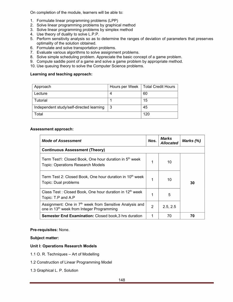
148
On completion of the module, learners will be able to:
1. Formulate linear programming problems (LPP) 2. Solve linear programming problems by graphical method 3. Solve linear programming problems by simplex method 4. Use theory of duality to solve L.P.P. 5. Perform sensitivity analysis so as to determine the ranges of deviation of parameters that preserves
optimality of the solution obtained. 6. Formulate and solve transportation problems. 7. Evaluate various algorithms to solve assignment problems. 8. Solve simple scheduling problem. Appreciate the basic concept of a game problem. 9. Compute saddle point of a game and solve a game problem by appropriate method. 10. Use queuing theory to solve the Computer Science problems.
Learning and teaching approach:
Approach Hours per Week Total Credit Hours
Lecture 4 60
Tutorial 1 15
Independent study/self-directed learning 3 45
Total 120
Assessment approach:
Mode of Assessment Nos.Marks Allocated
Marks (%)
Continuous Assessment (Theory)
Term Test1: Closed Book, One hour duration in 5th week
Topic: Operations Research Models 1 10
30
Term Test 2: Closed Book, One hour duration in 10th week
Topic: Dual problems 1 10
Class Test : Closed Book, One hour duration in 12th week
Topic: T.P and A.P 1 5
Assignment: One in 7th week from Sensitive Analysis and one in 13th week from Integer Programming
2 2.5, 2.5
Semester End Examination: Closed book,3 hrs duration 1 70 70
Pre-requisites: None.
Subject matter:
Unit I: Operations Research Models
1.1 O. R. Techniques – Art of Modelling
1.2 Construction of Linear Programming Model
1.3 Graphical L. P. Solution
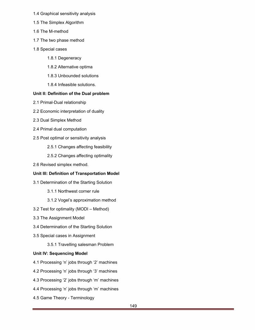
149
1.4 Graphical sensitivity analysis
1.5 The Simplex Algorithm
1.6 The M-method
1.7 The two phase method
1.8 Special cases
1.8.1 Degeneracy
1.8.2 Alternative optima
1.8.3 Unbounded solutions
1.8.4 Infeasible solutions.
Unit II: Definition of the Dual problem
2.1 Primal-Dual relationship
2.2 Economic interpretation of duality
2.3 Dual Simplex Method
2.4 Primal dual computation
2.5 Post optimal or sensitivity analysis
2.5.1 Changes affecting feasibility
2.5.2 Changes affecting optimality
2.6 Revised simplex method.
Unit III: Definition of Transportation Model
3.1 Determination of the Starting Solution
3.1.1 Northwest corner rule
3.1.2 Vogel’s approximation method
3.2 Test for optimality (MODI – Method)
3.3 The Assignment Model
3.4 Determination of the Starting Solution
3.5 Special cases in Assignment
3.5.1 Travelling salesman Problem
Unit IV: Sequencing Model
4.1 Processing ‘n’ jobs through ‘2’ machines
4.2 Processing ‘n’ jobs through ‘3’ machines
4.3 Processing ‘2’ jobs through ‘m’ machines
4.4 Processing ‘n’ jobs through ‘m’ machines
4.5 Game Theory - Terminology
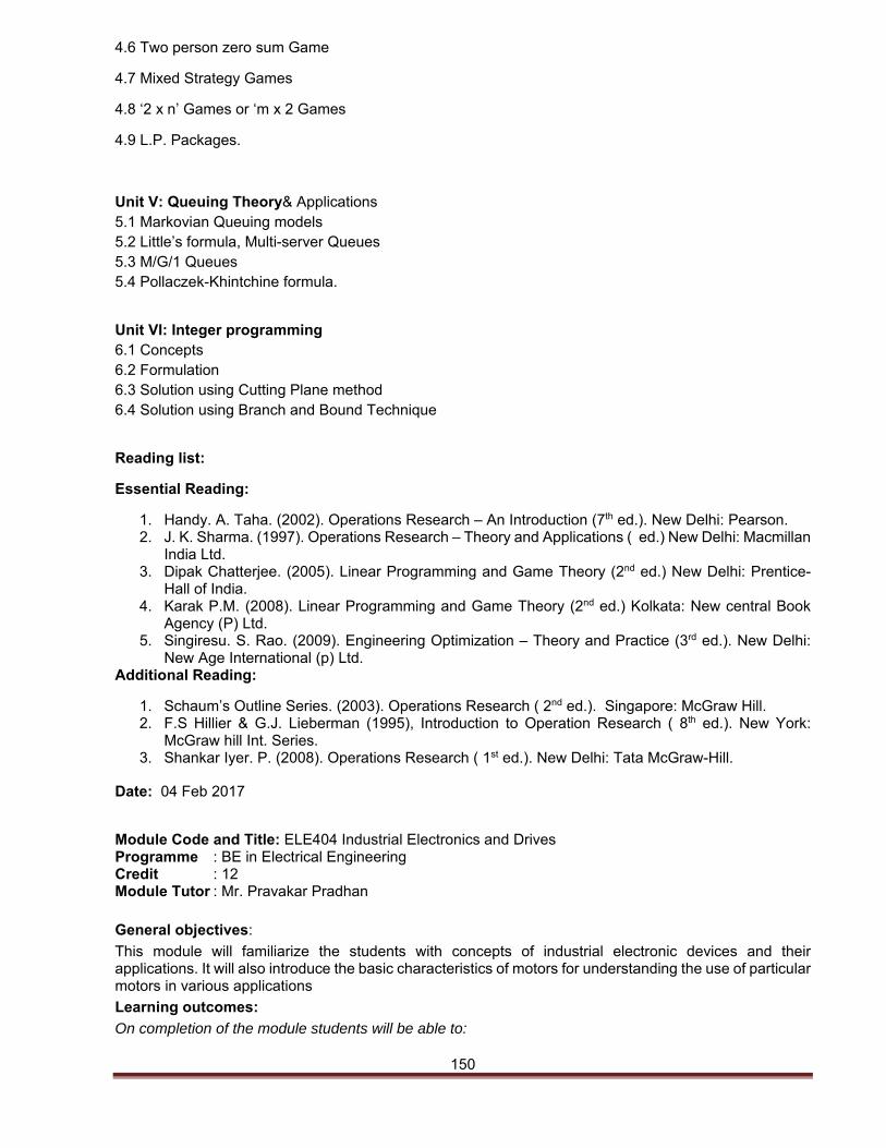
150
4.6 Two person zero sum Game
4.7 Mixed Strategy Games
4.8 ‘2 x n’ Games or ‘m x 2 Games
4.9 L.P. Packages.
Unit V: Queuing Theory& Applications 5.1 Markovian Queuing models 5.2 Little’s formula, Multi-server Queues 5.3 M/G/1 Queues 5.4 Pollaczek-Khintchine formula.
Unit VI: Integer programming 6.1 Concepts 6.2 Formulation 6.3 Solution using Cutting Plane method 6.4 Solution using Branch and Bound Technique
Reading list:
Essential Reading:
1. Handy. A. Taha. (2002). Operations Research – An Introduction (7th ed.). New Delhi: Pearson. 2. J. K. Sharma. (1997). Operations Research – Theory and Applications ( ed.) New Delhi: Macmillan
India Ltd. 3. Dipak Chatterjee. (2005). Linear Programming and Game Theory (2nd ed.) New Delhi: Prentice-
Hall of India. 4. Karak P.M. (2008). Linear Programming and Game Theory (2nd ed.) Kolkata: New central Book
Agency (P) Ltd. 5. Singiresu. S. Rao. (2009). Engineering Optimization – Theory and Practice (3rd ed.). New Delhi:
New Age International (p) Ltd. Additional Reading:
1. Schaum’s Outline Series. (2003). Operations Research ( 2nd ed.). Singapore: McGraw Hill. 2. F.S Hillier & G.J. Lieberman (1995), Introduction to Operation Research ( 8th ed.). New York:
McGraw hill Int. Series. 3. Shankar Iyer. P. (2008). Operations Research ( 1st ed.). New Delhi: Tata McGraw-Hill.
Date: 04 Feb 2017
Module Code and Title: ELE404 Industrial Electronics and Drives Programme : BE in Electrical Engineering Credit : 12 Module Tutor : Mr. Pravakar Pradhan
General objectives:
This module will familiarize the students with concepts of industrial electronic devices and their applications. It will also introduce the basic characteristics of motors for understanding the use of particular motors in various applications
Learning outcomes:
On completion of the module students will be able to:
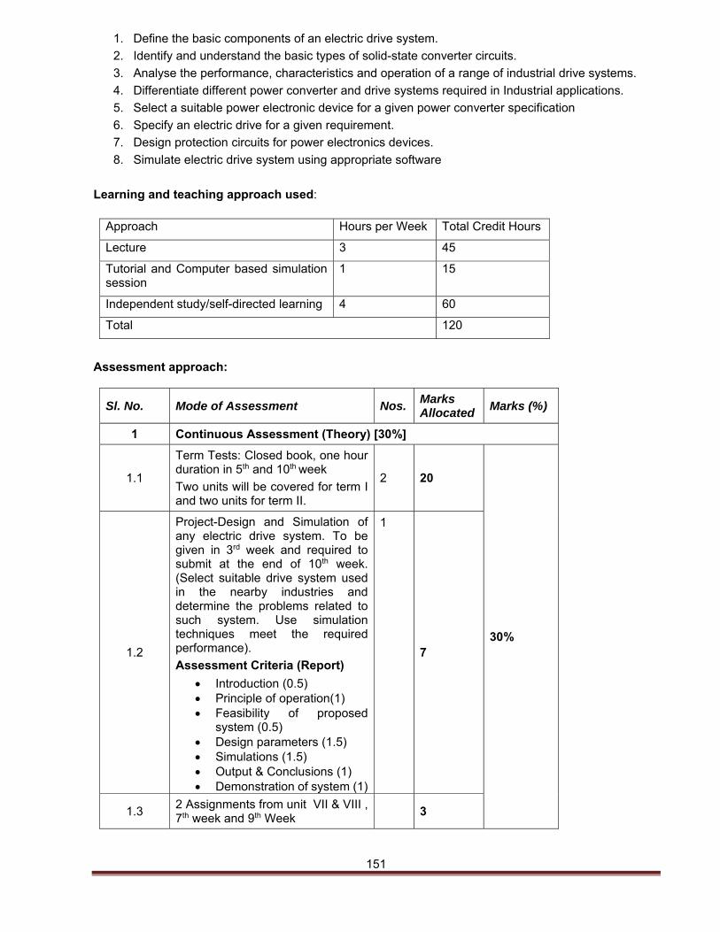
151
1. Define the basic components of an electric drive system.
2. Identify and understand the basic types of solid-state converter circuits.
3. Analyse the performance, characteristics and operation of a range of industrial drive systems.
4. Differentiate different power converter and drive systems required in Industrial applications.
5. Select a suitable power electronic device for a given power converter specification
6. Specify an electric drive for a given requirement.
7. Design protection circuits for power electronics devices.
8. Simulate electric drive system using appropriate software
Learning and teaching approach used:
Approach Hours per Week Total Credit Hours
Lecture 3 45
Tutorial and Computer based simulation session
1 15
Independent study/self-directed learning 4 60
Total 120
Assessment approach:
Sl. No. Mode of Assessment Nos. Marks Allocated
Marks (%)
1 Continuous Assessment (Theory) [30%]
1.1
Term Tests: Closed book, one hour duration in 5th and 10th week
Two units will be covered for term I and two units for term II.
2 20
30% 1.2
Project-Design and Simulation of any electric drive system. To be given in 3rd week and required to submit at the end of 10th week. (Select suitable drive system used in the nearby industries and determine the problems related to such system. Use simulation techniques meet the required performance).
Assessment Criteria (Report)
Introduction (0.5) Principle of operation(1) Feasibility of proposed
system (0.5) Design parameters (1.5) Simulations (1.5) Output & Conclusions (1) Demonstration of system (1)
1
7
1.3 2 Assignments from unit VII & VIII , 7th week and 9th Week
3
152
(Determining the construction, variable parameters & application of brushless dc drive system and stepping motors. It will consist of 5 numerical questions each in 7th and 9th week).
2 Semester End Examination 1 70 70%
Total 100%
Pre-requisite : ELE303 Power Electronics
Subject matter:
Unit I: Power Electronics Components and Basic Control Circuits:
1.1 Review of characteristics and limitations of 1.1.1 diode, 1.1.2 thyristor, 1.1.3 gate-turn-off-thyristor 1.1.4 bipolar transistor 1.1.5 MOSFET 1.1.6 IGBT 1.2 Selection of devices 1.2.1 Criteria for selecting drive components 1.2.2 Thermal considerations in selecting the motor 1.2.3 Selecting a Motor and power electronic converter
1.3 Gate/base circuits Unit II: Heating and Cooling Losses:
2.1 Thermal resistance
2.1.1 Generic geometry of heat flow via conduction
2.1.2 Thermal equivalent Circuits
2.1.3 Radiative thermal resistance
2.1.4 Convective Thermal resistance.
2.1.5 Combined Effects of Convection and radiation.
2.2 Transient thermal resistance
2.2.1 Concept of thermal resistance.
2.2.2 Calculation of transient thermal resistance.
2.2.3 Transient thermal resistance for multilayer structure.
2.3 Cooling techniques
2.3.1 Selection of Heat Sinks and their uses.
2.4 Model of switching losses.
2.4.1 Resistive load switching characteristics 2.4.2 Inductive load switching characteristics. 2.5 Selection of Motor Power rating 2.5.1 Thermal model of motor for heating and coolng 2.5.2 Classes of motor duty 2.5.3 Determination of motor rating
Unit III: Protection Circuits in Three Phase Rectifiers:
3.1 Review of main features of a three phase diode bridge rectifier
3.2 Identification of components storing energy under fault conditions
3.3 Design calculations to minimize the size of a selected protective capacitor system. Unit IV: Induction Motor Drives:
4.1 Control methods
153
4.1.1 Pole changing
4.1.2 Supply frequency control
4.1.3 Rotor resistance control
4.1.4 stator voltage control
4.1.5 Slip power recovery
4.2 Voltage drive and current drive
4.2.1 voltage source inverter (VSI) control
4.2.2 Current source inverter (CSI) control
4.3 Quasi-square wave
4.4 PWM inverter fed induction motor.
4.4.1 Regenerative voltage source inverter fed ac drive
4.4.2 Current controlled voltage source driven induction motor drive.
4.4.3 Sinusoidal PWM
4.5 Slip power recovery 4.5.1 Static Kramer drive 4.5.2 Static Scherbius Drive
4.6 cyclo-converter and harmonics.
Unit V: Synchronous Motor Drives:
5.1 D.C link
5.2 Starting techniques
5.2.1Damper winding
5.2.2 Cylindrical rotor wound field motor
5.2.3 Salient pole wound field motor
5.2.4 Permanent magnet motor
5.2.5 Synchronous reluctance motor
5.2.6 Hysteresis synchronous motor
5.3 Power converter. 5.3.1 Load commuted thyristor inverter 5.3.2 Variable frequency control of multiple synchronous motors. Unit VI: Brushed Dc Drive Systems:
6.1 Equations of motion and characteristics of operation
6.2 Methods of controlling using constant voltage and constant current techniques
6.2.1 phase control, with inner current loop
6.2.2 pulse width modulation control with inner current loop.
6.3 Integration into a complete servo system. 6.3.1 Applications in process rolling mills, winders, locomotives, larger cranes and elevators. 6.3.2 Drives for transportation, machine tools, and office equipment. Unit VII: Brushless Dc Drive Systems:
7.1 Types of motor construction of the two commonly used motor drives in industry
7.1.1 Permanent magnet ac motor drives
7.1.2 Sinusoidal PMAC motor drives fed from a current regulated voltage source inverter.
7.1.3 Brushless dc motor drives for servo applications.
7.2 Characteristics of the operation of motor and amplifier combinations, using two types of sensor feedback.
Unit VIII: Stepping drives systems:
8.1 Types of motor construction
8.2 Variable reluctance
8.3 Permanent magnet and Hybrid
8.4 Characteristics of motors
154
8.5 Special emphasis on torque curves and methods of controlling using open loop switching amplifiers.
Unit IX: Switched Reluctance Drives:
9.1 History
9.2 Linear analysis
9.2.1 single stack variable reluctance motor
9.2.2 multi-stack variable reluctance motor
9.2.3 Premanent magnet stepper motor
9.2.4 Hybrid stepper motor
9.3 Power electronics
9.3.1 Drive circuits for stepper motors
9.3.2 Unipolar drive for variable reluctance motors
9.3.3 Bipolar drive for Permanent magnet and Hybrid motors.
9.4 Practical motors
9.5 Low and high speed operation. Unit X: Simulation Techniques:
10.1 Simulate different circuits using Power Electronic Simulation Software.
Reading list:
Essential Reading:
1. Mohan, N., Undeland, T.M. & Robbins, W.P. (2009). Power Electronics: Converters, Applications and Design (2 ed.) New Delhi: Wiley India Pvt. Ltd
2. Bimbhra, P.S. (2000).Power Electronics ( 2 ed.). New Delhi :S Chand and Company.
3. Bose, B.K. (2005). Modern Power Electronics and AC Drives (2 ed.). New Delhi: Prentice-Hall of India Pvt. Ltd.
4. Krishnan, R. (2006).Electric Motor Drives – Modeling, Analysis and Control (4 ed.). New Delhi: Prentice-Hall of India Pvt. Ltd.
Additional Reading: 1. Dubey, G.K. (2000). Fundamentals of Electrical Drives (2 ed.). New Delhi: Narosa Publishing
House. Date: September 25, 2016 Module Code and Title : EMC403 Electrical Machine Design Programme : BE in Electrical Engineering Credit : 12 Module Tutor : Prem Kumar Nepal
General objectives:
This module will familiarize students with the basic concepts of the properties of electrical engineering materials, magnetic circuits and cooling of rotating electrical machines. Develop the basic concepts on the main design features of DC machines, transformers, induction machines and synchronous machines.
Learning outcomes:
On completion of the module students will be able to:
1. Derive the expression for the Quantity of cooling medium for air, hydrogen and water.
2. Interpret the properties of conducting materials - electrical conductivity, density, resistivity, Mechanical strength, reliability, draw ability, and solder ability, resistance to corrosion and thermal conductivity.
3. Compare the properties and cost of Aluminium, copper, iron and steel and their alloys used in electrical Engineering.
4. Calculate total mmf, mmf in air gap, net length of iron
155
5. Determine main dimensions of transformer, induction machines and synchronous machines.
6. Design of core, yoke, winding, armature winding and cooling tubes of transformers.
7. Derive output equations of transformer and induction machines and compute average flux densities in air gap and magnetizing currents
8. Design of rotor and stator slots for slip ring and cage type motors
9. Illustrate the effects of air gap and harmonics on the design of synchronous machines.
Learning and teaching approach:
Approach Hours per Week Total Credit Hours
Lecture 3 45
Tutorial 1 15
Independent study/self-directed learning
4 60
Total 120
.Assessment Approach:
Sl. No. Mode of Assessment Nos. Marks Allocated
Marks (%)
1 Continuous Assessment
1.1
Term Tests: Closed book, one hour duration in 5th and 10th week (Theory, Constructions, Derivations and calculations).
Two units will be covered for term I and three for term II . (Theory, Constructions, Derivations and calculations).
2 20
30
1.2 Assignments; at the end of 3rd and 8th week (Theory, Constructions, Derivations and calculations).
2 2x5
2 Semester End Examination (Closed book three hours).
1 70 70
Pre-requisites: EMC201 Electrical Machines – I and EMC302 Electrical Machines – II
Subject matter:
Unit I: Cooling of Rotating Electric Machines.
1.1 Explain the concept of Ratings, temperature rise, time curves 1.2 Explain cooling methods, cooling circuits, air, hydrogen and water cooling, direct cooling;
Quantity of cooling medium for air, hydrogen and water. 1.3 Electrical engineering materials and the basic principles of machine design including main
dimensions
Unit II: Electrical Calculations.
2.1 Electrical conductivity, density, resistivity, mechanical strength, reliability, draw ability, solder ability.
156
2.2 Resistance to corrosion; Thermal conductivity, cost, etc.; Aluminium, copper, iron and steel and their alloys used in electrical Engineering.
Unit III: Magnetic Calculations
3.1Calculation of total mmf, mmf in air gap, net length of iron;
3.2 Computation ofReal and apparent flux density, effects of leakage and saturation.
.
Unit IV: DC Machines 4.1 DC Machines, number of poles; length of air-gap; design of field system; inter-poles; commuter; and
brushes. 4.2 design of transformer tanks, laminations, leakage reactants, and temperature rise in transformer
Unit V: Transformers.
4.1 Determination of main dimension;
4.2 Design of core, yoke, winding and cooling tubes.
Unit VI: Induction Machines.
5.1Output equation; Average flux densities in air gap;
5.2Main dimension;
5.3Design of rotor and stator slots for slip ring and cage type motors;
5.4 Magnetizing currents; Design of armature winding.
Unit VII: Synchronous Machines.
6.1 Calculation of main dimensions.
6.2 Short circuit ratio and its influence on the design.
6.3 Air gap, harmonics and its effects on the design.
6.4 Elimination of harmonics.
6.5 Vibration of Electrical rotating machine:
Reading list:
Essential Reading:
1. Sawhney, A.K. (2014). A course in Electrical Machine Design (7 ed.). Delhi: Khanna Publishers.
2. Clayton & Hancock. (2004). Performance and Design of DC Machines (1 ed.). Delhi: Khanna Publishers.
3. Say, M.G. (2002). Performance and Design of DC Machines (3ed.). New Delhi: CBS Publishers and Distributors.
Additional Reading: 1. Upadhyay, K.G. (2011). Design of Electrical Machine (1 ed.).New Delhi: New Age International (P) Ltd. 2. Agarwal, R.K.(2015). Principles of Electrical Machine Design (7 ed.). Delhi: S K Kataria & Sons. 3. Deshpande, M.V. (2010). Design and Testing of Electrical Machines (4 ed.). New Delhi: PHI Learning Pvt. Ltd.
Date: February 4, 2017 Module Code and Title : SNP302 Digital Signal Processing Programme : BE in ELECTRONICS AND COMMUNICATION ENGINEERING Credit : 12 Module Tutor(s) : Ms.Dechen Lhamo
157
General objectives:
This module will enable the students to understand different types of digital signal processing techniques and tools, familiarize with the advanced transform namely discrete Z transform, Fast Fourier transform and Filters using appropriate software tool , and to apply transforms and DSP techniques to design systems of coding & decoding
Learning outcomes:
On completion of the module, students will be able to:
1. Describe the distinctions between analog, continuous-time, discrete-time and digital signals. 2. Apply the DSP tools and techniques, Discrete Z transform, Fast Fourier Transform for signal
analysis. 3. Design and analyse signals and systems. 4. Construct important filters FIR, IIR for systems and analysis. 5. Compare responses of the filters to signals, and categorize them. 6. Encode and decode information from signals. 7. Design signal processing algorithms to suite specific needs. 8. Use of signal processing tools for designing, implementing and simulation results.
Learning and teaching approach:
Approach Hours per Week Total Credit Hours
Lecture 3 45
Tutorial 1 15
Practical 2 30
Independent study/self-directed learning 2 30
Total 120 Assessment Approach:
Sl. No. Mode of Assessment Nos. Marks Allocated
Marks (%)
1 Continuous Assessment (Theory)
1.1 Term Test (closed book, 1 hour in the 5th and the 10th week of the semester)
2 10,10 25
1.2 Assignment (Problem solving based on the topics taught in the class)
2 2.5, 2.5
2 Practical
2.1
Introduction (theory, principle, significance and expected outcomes).
Materials requirement (materials used to do the practical with proper specification)
Step by step procedure followed by the student while conducting the experiment. This section should have enough detail so that reader can repeat the experiment).
Precaution (rules need to be followed in order to perform the practical with higher precision).
Results (state outcomes of the experiment but not interpret or draw conclusions about the data).Conclusion (state what student has learned by doing the experiment
8
1
3 2 2 2
25
2.2 Practical Exam 1 10
158
2.3 Viva-Voce 1 5
3 Semester End Examination 1 50 50
Pre-requisite: SNP201 Signals and Systems and MAT208 Engineering Mathematics IV
Subject Matter:
Unit I: Introduction 1.1. Overview of digital signal processing: need for DSP, advantages of DSP over analog
communication systems 1.2. Review of type of signals and systems (first unit of SNP201) 1.3. Discrete time signals and systems, LTI systems, stability and causality 1.4. Sampling of continuous time signals 1.5. Sampling rate conversion
Unit II: Mathematical Operations on Sequences
2.1. Linear Convolution of discrete signals: graphical method (overlap and add methods sliding tap methods) and analytical techniques, matrix methods I and II
2.2. some examples and solutions of LTI systems 2.3. programming examples using appropriate tool
Unit III: Discrete Fourier Transform
3.1. the Definition, Properties of Z transform, mapping between S-plane and Z-plane, Unit circle, convergence and ROC, Inverse z-transform, solution of difference equation using the one sided Z-transform
3.2. Relation between Z transform and Fourier transform of a sequence, Sampling of z transform 3.3. Discrete of Fourier transform, summary of the properties of Discrete Fourier transform Inverse
DFT, circular convolution, multiplication of DFT 3.4. Linear Filtering using DFT
Unit IV: Flow Graph and Computation of the Discrete Fourier Transform 4.1. Introduction 4.2. Goertzel Algorithm 4.3. Signal flow graph representation of digital network 4.4. Matrix representation of digital networks 4.5. Twiddle factor, Fast Fourier Transform, FFT algorithm, Radix 2 algorithm 4.6. Decimation in time and decimation in frequency algorithm, signal flow graph, butterflies 4.7. Computing an inverse DFT using FFT algorithm 4.8. Chirp z transform algorithm
4.9. programming examples using appropriate tool Unit-V: Finite Impulse Response (FIR) Filter
5.1. Introduction, comparison of FIR and IIR digital Filters 5.2. Properties of FIR Digital Filters, Magnitude and phase response of Digital Filters 5.3. Frequency response of linear phase FIR filter 5.4. Design technique of FIR filters: Design of Finite Impulse Response(FIR) filters, linear phase,
windows-rectangular, Berlet, Hamming and Blackman windows 5.5. Design of optimal Linear phase filters
Unit-VI: Infinite Impulse Response (IIR) Filter
6.1. Introduction 6.2. Design of infinite impulse response(IIR) filters from analog filters, IIR filter design by
approximation of derivatives 6.3. IIR filter design by Impulse Invariant Method 6.4. IIR filter design by the bilinear transformation 6.5. Butterworth filters, Chebyshev filters, Elliptic filters, Optimization method of IIR filters
Unit-VII: Realization of Digital Filters
159
7.1. Introduction 7.2. Basic structures for IIR filters 7.3. Basic structures of FIR filters 7.4. Principle of digital filter realization, structures of all-zero filters. 7.5. Basic realization block diagram and the signal flow graph 7.6. Some example of practical filters design. Computer aided filter design, MATLAB examples.
Unit-VIII: Application of Digital Signal Processing
8.1. Introduction 8.2. Voice processing 8.3. Application to radar 8.4. Application to image processing 8.5. Introduction to wavelets
List of Practical:
1. Generate Sine wave and hence Tan wave by writing program in C/C++ 2.4. Perform solution of given difference equation using the one sided Z-transform with programming
examples using appropriate tool 2.5. Demonstrate Chirap z-transform algorithm with programming examples using appropriate tool 2.6. Design and test of a FIR filter using programming examples using appropriate tool 2. and DSP Trainer kit 2.7. Design and test of an IIR filter using programming examples using appropriate tool 3. and DSP Trainer kit 4. Realize DTMF tone generator using DSP kits and code composer 5. Implement µ-law and A-law compounding with TMS320C54x DSP 6. Perform Fourier analysis of a given periodic signal 7. Implement Double Precision Complex FFT with TMS320c54x DSP
Reading List:
Essential Reading:
1. Salivahanan, S., Vallavaraj, A. & Gnanapriya, C (2005). Digital Signal Processing (16 ed.). New Delhi: Tata McGraw Hill.
2. Rabiner, L.R & Gold, B (2000). Theory and Application of Digital Signal Processing. New Delhi: Prentice Hall of India.
3. Proakis, J.G & Manolakis, D.G. (2007). Digital Signal Processing: Principles, Algorithms and Applications (4ed.). Pearson Education.
4. Mitra, S.K. (2011) “Digital Signal Processing – A Computer based approach” (4ed.). Tata McGraw-Hill.
5. Emmanual, C. et al. (2001). Digital Signal Processing: A Practical approach (2ed.). Pearson Education.
Additional Reading:
1. Hsu, H.P. & Ranjan, R., (2006). Signals and systems, New Delhi: Tata Mc.Graw Hill 2. Haykin, S. & Veen B.V., (1999). Signals and Systems. USA: John Wiley and sons. Lyons, R.G
(2010). Understanding digital signal processing (3ed.). Prentice Hall 3. DiStefano J.J. et al (2011). Digital Signal Processing: Schuam’s Outline Series (2 ed.). Prentice
Hall. 4. Meyar-Basse, U.(2007). Digital Signal Processing with FPGA (3rd ed.). India: Springer.
Date: February 24, 2016
Module Code and Title : PSS407 Advanced Power System Protection
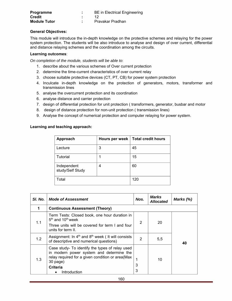
160
Programme : BE in Electrical Engineering Credit : 12 Module Tutor : Pravakar Pradhan
General Objectives:
This module will introduce the in-depth knowledge on the protective schemes and relaying for the power system protection. The students will be also introduce to analyse and design of over current, differential and distance relaying schemes and the coordination among the circuits.
Learning outcomes:
On completion of the module, students will be able to:
1. describe about the various schemes of Over current protection
2. determine the time-current characteristics of over current relay
3. choose suitable protective devices (CT, PT, CB) for power system protection
4. Inculcate in-depth knowledge on the protection of generators, motors, transformer and transmission lines
5. analyse the overcurrent protection and its coordination
6. analyse distance and carrier protection
7. design of differential protection for unit protection ( transformers, generator, busbar and motor
8. design of distance protection for non-unit protection ( transmission lines)
9. Analyse the concept of numerical protection and computer relaying for power system.
Learning and teaching approach:
Approach Hours per week Total credit hours
Lecture 3 45
Tutorial 1 15
Independent study/Self Study
4 60
Total 120
Sl. No. Mode of Assessment Nos. Marks Allocated
Marks (%)
1 Continuous Assessment (Theory)
1.1
Term Tests: Closed book, one hour duration in 5th and 10th week
Three units will be covered for term I and four units for term II.
2 20
40 1.2
Assignment: In 4th and 8th week ( It will consists of descriptive and numerical questions)
2 5,5
1.3
Case study- To identify the types of relay used in modern power system and determine the relay required for a given condition or area(Max 30 page)
Criteria Introduction
1
3
3
10
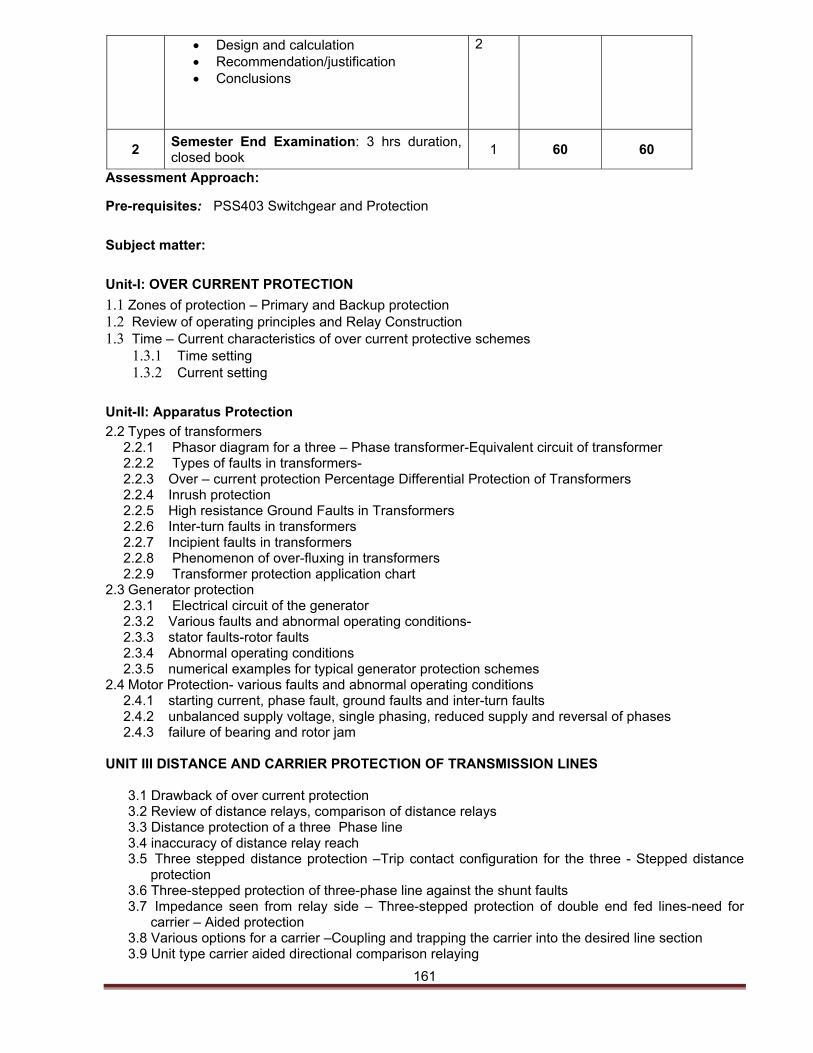
161
Assessment Approach:
Pre-requisites: PSS403 Switchgear and Protection
Subject matter:
Unit-I: OVER CURRENT PROTECTION
1.1 Zones of protection – Primary and Backup protection 1.2 Review of operating principles and Relay Construction 1.3 Time – Current characteristics of over current protective schemes
1.3.1 Time setting 1.3.2 Current setting
Unit-II: Apparatus Protection
2.2 Types of transformers 2.2.1 Phasor diagram for a three – Phase transformer-Equivalent circuit of transformer 2.2.2 Types of faults in transformers- 2.2.3 Over – current protection Percentage Differential Protection of Transformers 2.2.4 Inrush protection 2.2.5 High resistance Ground Faults in Transformers 2.2.6 Inter-turn faults in transformers 2.2.7 Incipient faults in transformers 2.2.8 Phenomenon of over-fluxing in transformers 2.2.9 Transformer protection application chart
2.3 Generator protection 2.3.1 Electrical circuit of the generator 2.3.2 Various faults and abnormal operating conditions- 2.3.3 stator faults-rotor faults 2.3.4 Abnormal operating conditions 2.3.5 numerical examples for typical generator protection schemes
2.4 Motor Protection- various faults and abnormal operating conditions 2.4.1 starting current, phase fault, ground faults and inter-turn faults 2.4.2 unbalanced supply voltage, single phasing, reduced supply and reversal of phases 2.4.3 failure of bearing and rotor jam
UNIT III DISTANCE AND CARRIER PROTECTION OF TRANSMISSION LINES
3.1 Drawback of over current protection 3.2 Review of distance relays, comparison of distance relays 3.3 Distance protection of a three Phase line 3.4 inaccuracy of distance relay reach 3.5 Three stepped distance protection –Trip contact configuration for the three - Stepped distance
protection 3.6 Three-stepped protection of three-phase line against the shunt faults 3.7 Impedance seen from relay side – Three-stepped protection of double end fed lines-need for
carrier – Aided protection 3.8 Various options for a carrier –Coupling and trapping the carrier into the desired line section 3.9 Unit type carrier aided directional comparison relaying
Design and calculation Recommendation/justification Conclusions
2
2 Semester End Examination: 3 hrs duration, closed book
1 60 60
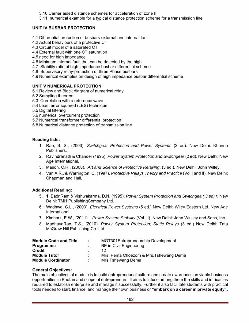
162
3.10 Carrier aided distance schemes for acceleration of zone ΙΙ 3.11 numerical example for a typical distance protection scheme for a transmission line
UNIT IV BUSBAR PROTECTION 4.1 Differential protection of busbars-external and internal fault 4.2 Actual behaviours of a protective CT 4.3 Circuit model of a saturated CT 4.4 External fault with one CT saturation 4.5 need for high impedance 4.6 Minimum internal fault that can be detected by the high 4.7 Stability ratio of high impedance busbar differential scheme 4.8 Supervisory relay-protection of three Phase busbars 4.9 Numerical examples on design of high impedance busbar differential scheme
UNIT V NUMERICAL PROTECTION 5.1 Review and Block diagram of numerical relay 5.2 Sampling theorem 5.3 Correlation with a reference wave 5.4 Least error squared (LES) technique 5.5 Digital filtering 5.6 numerical overcurrent protection 5.7 Numerical transformer differential protection 5.8 Numerical distance protection of transmission line Reading lists:
1. Rao, S. S., (2003). Switchgear Protection and Power Systems (2 ed). New Delhi: Khanna Publishers.
2. Ravindranath & Chander (1995). Power System Protection and Switchgear (2 ed). New Delhi: New Age International.
3. Mason, C.R., (2008). Art and Science of Protective Relaying, (3 ed.). New Delhi: John Willey.
4. Van A.R., & Warrington, C. (1997). Protective Relays Theory and Practice (Vol.I and II). New Delhi: Chapman and Hall.
Additional Reading:
5. 1. BadriRam & Vishwakarma, D.N. (1995). Power System Protection and Switchgea ( 3 ed) r. New Delhi: TMH PublishingCompany Ltd.
6. Wadhwa, C.L., (2003). Electrical Power Systems (5 ed.) New Delhi: Wiley Eastern Ltd. New Age International.
7. Kimbark, E.W., (2011). Power System Stability (Vol. II). New Delhi: John Wiulley and Sons, Inc.
8. MadhavaRao, T.S., (2010). Power System Protection; Static Relays (3 ed.) New Delhi: Tata McGraw Hill Publishing Co. Ltd.
Module Code and Title : MGT301Entrepreneurship Development Programme : BE in Civil Engineering Credit : 12 Module Tutor : Mrs. Pema Choezom & Mrs.Tshewang Dema Module Cordinator : Mrs.Tshewang Dema General Objectives: The main objectives of module is to build entrepreneurial culture and create awareness on viable business opportunities in Bhutan and scope of entrepreneurs. It aims to infuse among them the skills and intricacies required to establish enterprise and manage it successfully. Further it also facilitate students with practical tools needed to start, finance, and manage their own business or “embark on a career in private equity”.
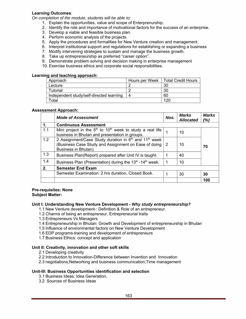
163
Learning Outcomes: On completion of the module, students will be able to:
1. Explain the opportunities, value and scope of Enterprenurship. 2. Identify the role and importance of motivational factors for the success of an enterprise. 3. Develop a viable and feasible business plan. 4. Perform economic analysis of the projects. 5. Apply the procedures and formalities for New Venture creation and management 6. Interpret institutional support and regulations for establishing or expanding a business 7. Modify intervening strategies to sustain and manage the business growth. 8. Take up entrepreneurship as preferred “career option”. 9. Demonstrate problem solving and decision making in enterprise management 10. Exercise business ethics and corporate social responsibilities.
Learning and teaching approach:
Approach Hours per Week Total Credit Hours Lecture 2 30 Tutorial 2 30 Independent study/self-directed learning 4 60 Total 120
Assessment Approach:
Mode of Assessment Nos.
Marks Allocated
Marks (%)
1. Continuous Assessment 1.1 Mini project in the 5th to 10th week to study a real life
business in Bhutan and presentation in groups. 1 10
70
1.2 2 Assignment/Case Study duration in 6th and 11th week (Business Case Study and Assignment on Ease of doing Business in Bhutan)
2 10
1.3 Business Plan(Report) prepared after Unit IV is taught. 1 40
1.4 Business Plan (Presentation) during the 13th -14th week. 1 10
2. Semester End Exam Semester Examination: 2 hrs duration, Closed Book. 1 30 30
100 Pre-requisites: None Subject Matter: Unit I: Understanding New Venture Development - Why study entrepreneurship?
1.1 New Venture development-: Definition & Role of an entrepreneur. 1.2 Charms of being an entrepreneur, Entrepreneurial traits 1.3 Entrepreneurs Vs Managers 1.4 Entrepreneurship in Bhutan: Growth and Development of entrepreneurship in Bhutan 1.5 Influence of environmental factors on New Venture Development 1.6 EDP programs-training and development of entrepreneurs 1.7 Business Ethics: concept and application
Unit II: Creativity, innovation and other soft skills
2.1 Developing creativity 2.2 Introduction to Innovation-Difference between Invention and Innovation 2.3 negotiations;Networking and business communication;Time management
Unit-III: Business Opportunities identification and selection
3.1 Business Ideas: Idea Generation, 3.2 Sources of Business Ideas
164
3.3 Emerging opportunities in Bhutan: manufacturing, trading, services (including hospitality and tourism, IT, ITES-Information Technology Enabled Services and knowledge based business opportunities)
3.4 Project identification and formulation 3.5 Classification of projects 3.6 Feasibility studies in context of Bhutanese business environment.
Unit IV: Business Plan
4.1 Need and importance of Business Plan 4.2 Economic Analysis of projects 4.3 Ccomponents of Bbusiness plan: Marketing Plan; Production & Technical Plan; Organization and
Management Plan; Financial Plan. 4.4 Guide to present the Business Plan
Unit V: New venture Process & Problems-Challenges
5.1 Procedures and formalities for setting up new enterprise, Regulations governing new ventures: 5.2 Stages of new venture development, Success factors of New Venture Development 5.3 Why new ventures fail-Causes and Remedies.
Unit VI: Promoting a New Venture –Environmental Support
6.1 Business Incubators-Role of business incubation centers. 6.2 Incentives and concessions for new venture 6.3 Financial institutions supporting entrepreneurs and new venture development
Unit VII: Leadership and Growth Management
7.1 General Management: Managing a small scale business 7.2 Functional Management: Marketing, Finance and Human resource. 7.3 Entrepreneurial leadership-Building successful teams 7.4 Dimensions of Business growth and dynamics involved-different growth objectives
7.5 Different risks faced during growth stage-Strategies to avoid those risks Reading Lists: Essential Reading:
1. Hisrich, R.D, Perters & Michal,P.(2005) Entrepreneurship (5th Edition). Tata McGraw Hill. 2. Thomas & Zimmerer. Essentials of entrepreneurship and small business management. Prentice
Hall of India. 3. Jeffry A. Timmons and Stephen Spinelli. (2004). New Venture Creation: Entrepreneurship for the
21st Century. McGraw-Hill/Irwin: NY 4. Ries E.( 2011) The Lean Startup: How Constant Innovation Creates Radically Successful
Businesses. Penguin United Kingdom. 5. Gupta, C.B. & Srinivasan, N.P(2014) Entrepreneurial Development. Sultan Chand & Sons, India.
Additional Reading:
1. Desai, V.(2005) Dynamics of Entrepreneurial Development and management (5th Edition). Himalaya Publishing House.
2. Mary C. (2005) Entrepreneurship in action(2nd Edition). Prentice Hall India. 3. Timmons, J. A and Spinelli, S. (2004). New Venture Creation (6th Ed.) New York. Mc-Graw Hill. 4. Hoffman R & Kidder D. (2013) The Startup Playbook: Secrets of the Fastest-Growing Startups
from Their Founding Entrepreneurs. Chronicle Books. 5. W.Ed McMullan and Wayne A. Long. (1990).Developing New Ventures: The entrepreneurial
option. Harcourt Brace Jovanovich,Inc: USA. 6. Economic Development Policy of The Kingdom of Bhutan (2010).
Date: 4th February 2017
Module Code and Title : PSS408 Power Market and Trading
165
Programme : BE in Electrical Engineering
Credit : 12
Module Tutor : Roshan Chhetri
General Objectives:
The module is to familiarize students to understand power sectors, pricing methods, tariffs, impacts, risk, hazards and remedial measures.
Learning outcomes:
On completion of the module, learners will be able to:
1. Explore Bhutanese power sectors, electricity acts, national policies and guidelines under these acts.
2. Discuss tariffs; compare different tariff structure for different loads. 3. Explore social, economic and environmental impact of energy system(discuss in context to Bhutan
and other countries) 4. Explain the concept of power system restructuring and its importance in present scenario 5. Identify different market and trading models / arrangements, open access, key market entities- ISO,
Genco, Transco, Disco, Retail co. 6. Differentiate between dynamic, spot pricing and real time pricing, Dispatch based pricing, Power
flows and prices. 7. Identify various impact of energy system to the environment and their remedial measures. 8. Identify risk, hazard and its remedial measures. 9. critically evaluate the viability of constructing individual plants in market conditions 10. Assess the impact of day-ahead market on the profitability of individual plants with special
emphasis on flexibility in power production 11. Independently investigate and discuss the arguments (flexible) mechanisms of emissions trading,
and the impact on the power market. 12. investigate upcoming trends in the market mechanisms, with special emphasis on network energy
market, and the effect that has on the market price of energy, and strategic decisions in the energy sector
Learning and teaching approach:
Lectures introduce concepts and provide a broad background; demonstrations are used to clarify particular points of detail or to illustrate concepts. Directed reading and assigned problems develop learning at a pace appropriate to the individual student. Tests and worksheets are used to help students to monitor their own progress through the module.
Approach Hours per week Total credit hours
Lecture 3 45
Tutorial 1 15
Independent learning/ self-study
4 60
Total 120
166
2.1 Assessment approach:
Pre-requisite:
Subject Matter
UNIT I: Introduction
1.1 Demand and Supply, 1.2 Vertically integrated monopolies and Competitive energy companies, 1.3 Price formation mechanisms, 1.4 Security of supply, 1.5 Power and competitiveness, 1.6 Hydro market
UNIT II INTRODUCTION TO POWER SECTOR STRUCTURE IN BHUTAN
2.1 Introduction to various institutions in Bhutanese Power sector policy bodies, utilities and regulators 2.2 Salient features of Electricity act of Bhutan (i.e. Act 2001), various National policies and guidelines
under this act. 2.3 Grid code regulation of Bhutan
UNIT III: POWER SECTOR ECONOMICS AND REGULATION
3.1 Power sector restructuring 3.2 Power markets deregulation, 3.3 Power market models 3.4 Partially and fully opened market 3.5 Utilities unbundling: vertical and horizontal, Separation of generation, transmission, distribution and
supply services 3.6 Different methods of comparing investment options, 3.7 calculate life cycle cost , annual rate of return , Internal Rate of Return(IRR) and Net Present
Value(NPV) of power project, 3.8 Short term and long term marginal costs, 3.9 Different financing options for the power sector
UNIT IV: PRICE FORMATION
4.1 Tariff system
Sl. No. Mode of Assessment Nos. Marks Allocated
Marks (%)
1 Continuous Assessment (Theory)
1.1
Term Tests:Closed book, one hour duration in 5th and 10th week
Two units will be covered for term I and three units for term II.
2 20 30
1.2 Assignment 4th week 1 10
1.3 Project work and presentation
2 Continuous Assessment (Practical)
2.1 Regular Practical Class: 2 hrs each every week
2.2 Practical Exam and Viva: 2 Hrs at 14th week
2.3 Project work (computer based simulation) 7th week
3 Semester End Examination: 2 hrs duration, closed book
1 70 70
167
4.2 Different tariff principles (marginal cost, cost to serve, average cost), 4.3 Consumer tariff structures and considerations, different consumer categories, telescopic tariff, fixed
and variable charges, time of day, interruptible tariff, different tariff based penalties and incentives etc., Subsidy and cross subsidy, life line tariff,
4.4 Comparison of different tariff structures for different load patterns. 4.5 Effect of renewable energy and captive power generation on tariff. 4.6 Determination of tariff for renewable energy.
UNIT V: POWER SECTOR RESTRUCTURING AND MARKET REFORM
5.1 Different industry structures and ownership and management models for generation, transmission and distribution. Competition in the electricity sector- conditions, barriers, different types, benefits and challenges Latest reforms.
5.2 Different market and trading models / arrangements, open access, key market entities- ISO, Genco, Transco, Disco, Retail co.
5.3 Power market types, Energy market, Ancillary service market, transmission market, forward and real time markets, and market power.
UNIT VI: ELECTRICITY MARKETS PRICING AND NON-PRICE ISSUES
6.1 Electricity price basics, Market Clearing price (MCP), Zonal and locational area clearing price (ACP).
6.2 Dynamic, spot pricing and real time pricing, Dispatch based pricing, Power flows and prices. 6.3 Optimal power flow Spot prices for real and reactive power. Unconstrained real spot prices,
constrains and real spot prices. 6.4 Non price issues in electricity restructuring (quality of supply and service, standards of
performance by utility, environmental and social considerations) 6.5 Global experience with electricity reforms in different countries. 6.6 Cost of new entrant to energy market I. Bilateral markets. Spot market. Day-ahead market 6.7 Cost of new entrant to energy market II. Pool system, Obligatory and voluntary pool 6.8 Regional integration 6.9 Privileged producers. Renewable energy sources. Feed-in tariffs. Avoided costs. Green
certificates.
UNIT VI: IMPACT OF ENERGY SYSTEMS ON ENVIRONMENT
7.1 Environmental degradation due to energy production and utilization, Primary and Secondary pollution such as SOx, NOx, SPM in air, thermal and water pollution, depletion of ozone layer, global warming, biological damage due to environmental degradation.
7.2 Emission (SOx, NOx, CO2) markets and its influence on energy markets. 7.3 Sociological and Economical problems due to Thermal and other energy projects. Physiological,
ecological and environmental and health problems due to energy plants. 7.4 Potential sources of Pollution in power plant (Hydro, thermal, nuclear etc), Impacts of pollution on
land, water and air. 7.5 Methods of Environmental Impact Assessment.
UNIT VIII: RISK AND HAZARD MANAGEMENT IN ENERGY SECTOR
8.1 Hazard Identification & Safety Audit 8.2 Safety code and safety regulation of Bhutan 8.3 Methods for Hazard Identification: Fault/Event tree Analysis; HAZOP; FMEA 8.4 Hazard Indices, Hazard Quantification 8.5 General Modeling Approaches, Empirical Tools; Computational (Numerical) Codes;
Phenomenological Models 8.6 Explosion Hazards, Explosion Fundamentals, Variety of modeling approaches for different
categories of explosions 8.7 Fire Hazards, Variety of modeling approaches for different category of fires: Jet Fire, Pool fire,
BLEVE, etc. 8.8 Dispersion Hazards, Heavy Gas Dispersion; Atmospheric Dispersion 8.9 Quantified Risk Analysis (QRA), Approach and practical examples 8.10 Hazard Elimination/Mitigation, General Concepts with practical Engineering examples.
168
Essential Reading
1. Krishnan, N.V, (1996).Safety in industry (1 ed.) New Delhi: Jaico Publishing House.
2. Cooper, W. (1986). Electrical Safety Engineering (2 ed.) London: Butterworth
3. Fowler, J.M. (1975). Energy and Environment (2 ed.). TMH Publication
4. Foell, W.K. (1997). Management of Energy-Environment Systems: Methods and Case Studies. New Delhi: John Wiley & Sons
Additional Reading
1. Mary, C. & Dennis, N (2005). Electrical Safety Handbook (4ed). New Delhi: McGraw Hill Professional.
2. Hunt, S. (2002). Making Competition Work in Electricity. New Delhi:John Wiley Inc 3. Regulation in infrastructure Services: Progress and the way forward - TERI, 2001 4. Electricity Act of Bhutan 2001 (www.bea.gov.bt)
Date: December 30, 2016
Appendix–I: In-Service BE. Electrical Engineering Programme
1. Appraisal of In-service programme
In 2011 three years in-service Bachelor of Engineering in Electrical programme was introduced at College
of Science and Technology. This is the first review of the programme since its introduction. So far from
year 2011 to 2016, only twelve candidates had enrolled to the programme, out of which three candidates
have successfully completed the course.
It is observed that the majority of the enrolled candidates are from corporate sectors, few on self-finance
mode and not a single candidate (in electrical) from the government sectors is funded for the programme.
The enrolment statistics indicates that the in-service program has not been able to attract the candidates
in large numbers. However, the college strongly commits to continue offering the programme to support
the career enhancement of those interested prospective candidates working in various organizations. The
continuation of the in-service programme does not have any resource implications to the college; this is
the rationale behind the strong commitment to continue offering the programme.
The induction into the three-year degree programme is considered based on the Diploma in Electrical
Engineering (of three, two & half and two years) programme offered by Jigme Namgyal Engineering
College (JNEC). The recognition of prior learning (RPL) is proposed by mapping the curriculum structure
of degree with the existing two years diploma offered by JNEC. The proposed review documents prepared
by JNEC have been considered for RPL. The 12 modules could be considered for recognition for prior
learning (RPL), which is 23.81 % (120/504) of the total credits in degree programme. The details of
modules proposed for RPL and the gap analysis of the module contents is shown in Table 1 and Table 2
respectively;
Table 1: Modules recognized for prior learning
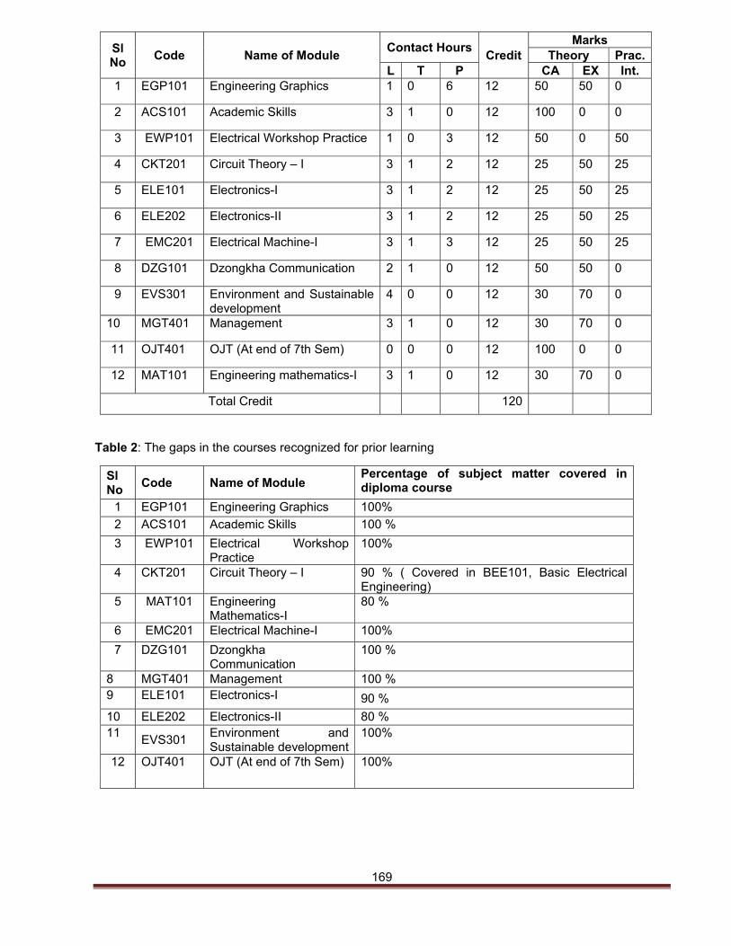
169
Sl No
Code Name of Module Contact Hours
Credit Marks
Theory Prac.L T P CA EX Int.
1 EGP101 Engineering Graphics 1 0 6 12 50 50 0
2 ACS101 Academic Skills 3 1 0 12 100 0 0
3 EWP101 Electrical Workshop Practice 1 0 3 12 50 0 50
4 CKT201 Circuit Theory – I 3 1 2 12 25 50 25
5 ELE101 Electronics-I 3 1 2 12 25 50 25
6 ELE202 Electronics-II 3 1 2 12 25 50 25
7 EMC201 Electrical Machine-I 3 1 3 12 25 50 25
8 DZG101 Dzongkha Communication 2 1 0 12 50 50 0
9 EVS301 Environment and Sustainable development
4 0 0 12 30 70 0
10 MGT401 Management 3 1 0 12 30 70 0
11 OJT401 OJT (At end of 7th Sem) 0 0 0 12 100 0 0
12 MAT101 Engineering mathematics-I 3 1 0 12 30 70 0
Total Credit 120
Table 2: The gaps in the courses recognized for prior learning
Sl No
Code Name of Module Percentage of subject matter covered in diploma course
1 EGP101 Engineering Graphics 100%
2 ACS101 Academic Skills 100 %
3 EWP101 Electrical Workshop Practice
100%
4 CKT201 Circuit Theory – I 90 % ( Covered in BEE101, Basic Electrical Engineering)
5 MAT101 Engineering Mathematics-I
80 %
6 EMC201 Electrical Machine-I 100%
7 DZG101 Dzongkha Communication
100 %
8 MGT401 Management 100 % 9 ELE101 Electronics-I 90 %
10 ELE202 Electronics-II 80 % 11
EVS301 Environment and Sustainable development
100%
12 OJT401 OJT (At end of 7th Sem) 100%
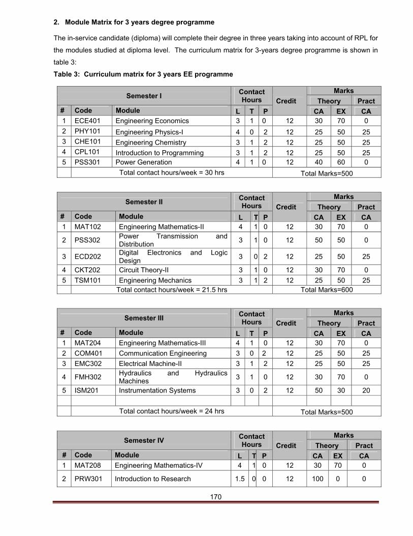
170
2. Module Matrix for 3 years degree programme
The in-service candidate (diploma) will complete their degree in three years taking into account of RPL for
the modules studied at diploma level. The curriculum matrix for 3-years degree programme is shown in
table 3:
Table 3: Curriculum matrix for 3 years EE programme
Semester I Contact Hours Credit
Marks
Theory Pract # Code Module L T P CA EX CA 1 ECE401 Engineering Economics 3 1 0 12 30 70 0
2 PHY101 Engineering Physics-I 4 0 2 12 25 50 25 3 CHE101 Engineering Chemistry 3 1 2 12 25 50 25 4 CPL101 Introduction to Programming 3 1 2 12 25 50 25 5 PSS301 Power Generation 4 1 0 12 40 60 0
Total contact hours/week = 30 hrs Total Marks=500
Semester II Contact Hours Credit
Marks
Theory Pract # Code Module L T P CA EX CA 1 MAT102 Engineering Mathematics-II 4 1 0 12 30 70 0
2 PSS302 Power Transmission and Distribution
3 1 0 12 50 50 0
3 ECD202 Digital Electronics and Logic Design
3 0 2 12 25 50 25
4 CKT202 Circuit Theory-II 3 1 0 12 30 70 0
5 TSM101 Engineering Mechanics 3 1 2 12 25 50 25 Total contact hours/week = 21.5 hrs Total Marks=600
Semester III Contact Hours Credit
Marks
Theory Pract # Code Module L T P CA EX CA 1 MAT204 Engineering Mathematics-III 4 1 0 12 30 70 0
2 COM401 Communication Engineering 3 0 2 12 25 50 25
3 EMC302 Electrical Machine-II 3 1 2 12 25 50 25
4 FMH302 Hydraulics and Hydraulics Machines
3 1 0 12 30 70 0
5 ISM201 Instrumentation Systems 3 0 2 12 50 30 20
Total contact hours/week = 24 hrs Total Marks=500
Semester IV Contact Hours Credit
Marks
Theory Pract # Code Module L T P CA EX CA 1 MAT208 Engineering Mathematics-IV 4 1 0 12 30 70 0
2 PRW301 Introduction to Research 1.5 0 0 12 100 0 0
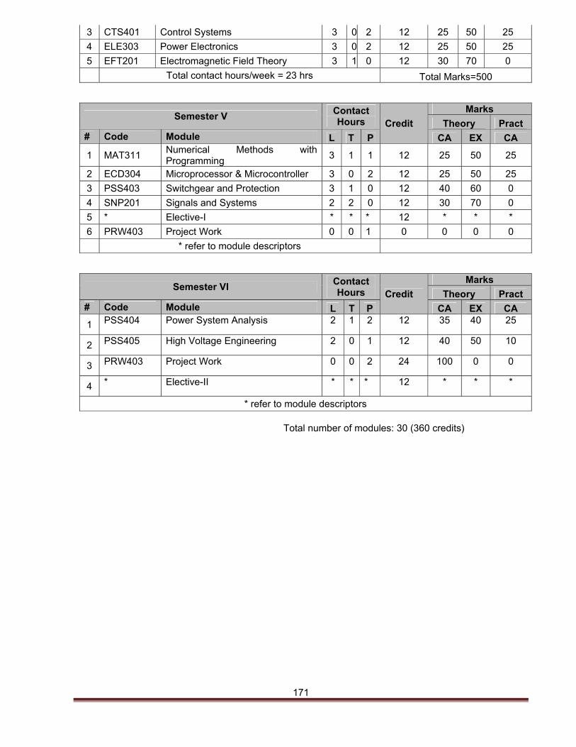
171
3 CTS401 Control Systems 3 0 2 12 25 50 25
4 ELE303 Power Electronics 3 0 2 12 25 50 25
5 EFT201 Electromagnetic Field Theory 3 1 0 12 30 70 0
Total contact hours/week = 23 hrs Total Marks=500
Semester V Contact Hours Credit
Marks
Theory Pract # Code Module L T P CA EX CA
1 MAT311 Numerical Methods with Programming
3 1 1 12 25 50 25
2 ECD304 Microprocessor & Microcontroller 3 0 2 12 25 50 25
3 PSS403 Switchgear and Protection 3 1 0 12 40 60 0
4 SNP201 Signals and Systems 2 2 0 12 30 70 0
5 * Elective-I * * * 12 * * *
6 PRW403 Project Work 0 0 1 0 0 0 0
* refer to module descriptors
Semester VI Contact Hours Credit
Marks
Theory Pract # Code Module L T P CA EX CA
1 PSS404 Power System Analysis 2 1 2 12 35 40 25
2 PSS405 High Voltage Engineering 2 0 1 12 40 50 10
3 PRW403 Project Work 0 0 2 24 100 0 0
4 * Elective-II * * * 12 * * *
* refer to module descriptors Total number of modules: 30 (360 credits)