ARTICLES

Snowball Earth prevention by dissolvedorganic carbon remineralizationW. Richard Peltier1, Yonggang Liu1 & John W. Crowley1

The ‘snowball Earth’ hypothesis posits the occurrence of a sequence of glaciations in the Earth’s history sufficiently deep thatphotosynthetic activity was essentially arrested. Because the time interval during which these events are believed to haveoccurred immediately preceded the Cambrian explosion of life, the issue as to whether such snowball states actuallydeveloped has important implications for our understanding of evolutionary biology. Here we couple an explicit model ofthe Neoproterozoic carbon cycle to a model of the physical climate system. We show that the drawdown of atmosphericoxygen into the ocean, as surface temperatures decline, operates so as to increase the rate of remineralization of a massivepool of dissolved organic carbon. This leads directly to an increase of atmospheric carbon dioxide, enhanced greenhousewarming of the surface of the Earth, and the prevention of a snowball state.

During the Neoproterozoic era of the Earth’s history, the carboncycle exhibited a sequence of oscillation-like variations that includeddecreases of d13C to levels that have been interpreted to imply theoccurrence of intense snowball glaciations1 during which photosyn-thetic activity essentially ceased2–4. Such events would have stronglyaffected the evolution of eukaryotic life and this has led to suggestionsthat this extreme interpretation of the observed variability in thecarbon cycle could be unwarranted5,6. We have developed a coupledmodel of the co-evolution of Neoproterozoic climate and the carboncycle that provides an alternative interpretation to the ‘hard snow-ball’ hypothesis of the origin of the observed d13C variations. Thismodel links a previously developed model of the Neoproterozoicphysical climate system7,8 to a recently developed model of the carboncycle9 for the same time interval. The coupled model is shown tosupport a limit cycle oscillation in which the temperature depen-dence of the solubility of oxygen in sea water controls the rate ofremineralization of organic carbon such that the level of atmo-spheric CO2 is prevented from becoming sufficiently low to allow ahard snowball state to occur. The model also satisfies the timescaleand continental ice volume constraints that have been inferred tocharacterize these glaciation events, as well as the magnitude of thecarbon cycle excursions when an appropriate biogeochemicaldependence of photosynthetic carbon isotopic fractionation isassumed.

The sequence of intense glaciations that occurred during theCryogenian period of the Neoproterozoic era—a period that beganapproximately 850 million years (Myr) ago and which endedapproximately 635 Myr ago with the onset of the Ediacaranperiod—is currently an intense focus of interdisciplinary activity10.Evolutionary biologists and palaeontologists11,12 are interested in thisera because it preceded the Cambrian explosion of life, during whicheukaryotic biological diversity proliferated. Climate dynamicists13–18

have been attracted by the challenge posed by the appearance in thegeological record of continental-scale glaciation that is suggested tohave reached sea level in equatorial latitudes at some locations.Sedimentologists19–21 and geochronologists22 have worked on theglobal-scale correlation of glacial units across the present-day con-tinents, during a time of intense tectonic activity involving the break-up of the supercontinent of Rodinia. However, many important

questions are still unresolved. In particular, how many glaciationsactually occurred during the Cryogenian period is currently uncer-tain. Figure 1, a revised and extended version of previously publishedsketches23–25 of the evolution of d13C over the most recent billionyears of the Earth’s history, illustrates the connection in time betweenthis measure of climate variability, major tectonic events, and periodsof intense glaciation.

The nature of Cryogenian glacial episodes

Although some recent work has championed the notion that onlythree major glaciations occurred during this period23—the Sturtianglaciation at 723z16

{10 Myr ago, the Marinoan glaciation between 659and 637 Myr ago, and the Gaskiers glaciation at approximately582 Myr ago—there remain significant issues concerning the syn-chroneity of these events as inferred on the basis of the stratigraphicrecord from different continents. The chronological control upon theSturtian glaciation, in particular, now suggests that it consisted of atleast two distinct glacial episodes22. Evidence from the HuqfSupergroup of Oman has recently been interpreted to imply thatno hard snowball glaciation event could have occurred19–21.Similarly, the duration of individual glacial episodes remainsunknown (although it has been speculated to be between 4 and 30million years4), as is the answer to the question of whether each of theglacial episodes consisted of a single ice advance and retreat or ofmultiple such events.

A previously proposed model of Neoproterozoic climate suggestedthe plausibility of a ‘‘slushball’’ solution in which a significant regionof open water could have persisted at the Equator during each ofthese events. This model has been criticized26 on the basis of the claimthat it could not explain the inferred requirement of the geologicalrecord for the occurrence of episodes of glaciation that lasted at least4 Myr. This is the point of departure for the analyses described in thispaper. Our target has been the question posed by the carbon isotopicvariability depicted qualitatively in Fig. 1. Whereas subsequent to theNeoproterozoic era the carbon cycle appears to have been operatingin a quasi-equilibrium mode9, during the Neoproterozoic it appearsto have been operating in an out-of-equilibrium mode that is pecu-liar to this interval of the Earth’s history. This mode of behaviour wasrecently suggested9 to have arisen as a consequence of a significant

1Department of Physics, University of Toronto, Toronto, Ontario M5S 1A7, Canada.

Vol 450 | 6 December 2007 | doi:10.1038/nature06354

813Nature ©2007 Publishing Group

imbalance between the mass of carbon stored in the Neoproterozoicocean in the organic and inorganic forms. Atmospheric oxygen couldhave provided an important link between the carbon cycle and cli-mate but no detailed discussion was provided9. The purpose of theanalyses reported here is to elaborate a plausible linkage and toinvestigate the extent to which this may shed light upon the stateof the Earth’s physical climate system during this critical period forbiological evolution.

Coupled carbon cycle–climate evolution

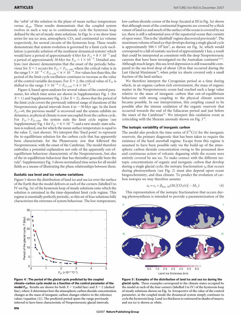
A schematic of the model we have developed for this purpose isshown in Fig. 2, consisting of three primary elements: a model ofthe carbon cycle9, a model of the physical climate system (consistingof surface energy balance and sea-ice components8), and a detailedmodel of continental-scale glaciation (the University of TorontoGlacial Systems Model; ref. 27). The mathematical details of thecarbon cycle component of the complete coupled model, whichinvolve a significant extension of the model of ref. 9, are describedin the Supplementary Information). To link these models we expli-citly incorporated a dependence of the remineralization flux J21

(Fig. 2), through which organic carbon is converted to inorganiccarbon, upon the (temperature-dependent) solubility of oxygen insea water:

J21~J21e1{F21(T{Te)½ � ð1Þ

In this expression, T is the mean surface temperature of the planetdetermined by the physical climate model and Te is the equilibriumtemperature at which the remineralization flux J21 equals its equi-librium value. For a discussion of the physical significance of the

control parameter F21, please see Methods. A primary assumptionof the present version of the model is that the variations in

Late Quaternaryglacial era

Cambrianexplosion

Glaciationof Pangaea

Cryogenian Ediacaran

Neoproterozoic Phanerozoic

Age (Myr ago)

1,000 800 600 400 200 0

Glacial eras

Tectonic events

Incr

easi

ng o

rgan

ic b

uria

l

U–Pbages

Shuramanomaly

Marinoan glaciations

Sturtian glaciations

Gaskiers glaciationSnowball

events?

–5

0

10

δ13 C

(‰V

PD

B)

–10

5

Mid-Proterozoicnon-glacial era

Neoproterozoicglacial era

Late Palaeozoicglacial era

Assembly ofRodinia

Rifting anddispersal of

Rodinia

Assemblyof Pangaea

Rifting anddispersal

of Pangaea

Bitter S

pringsstage

Trezonaanom

aly

Mai eberg

anomaly

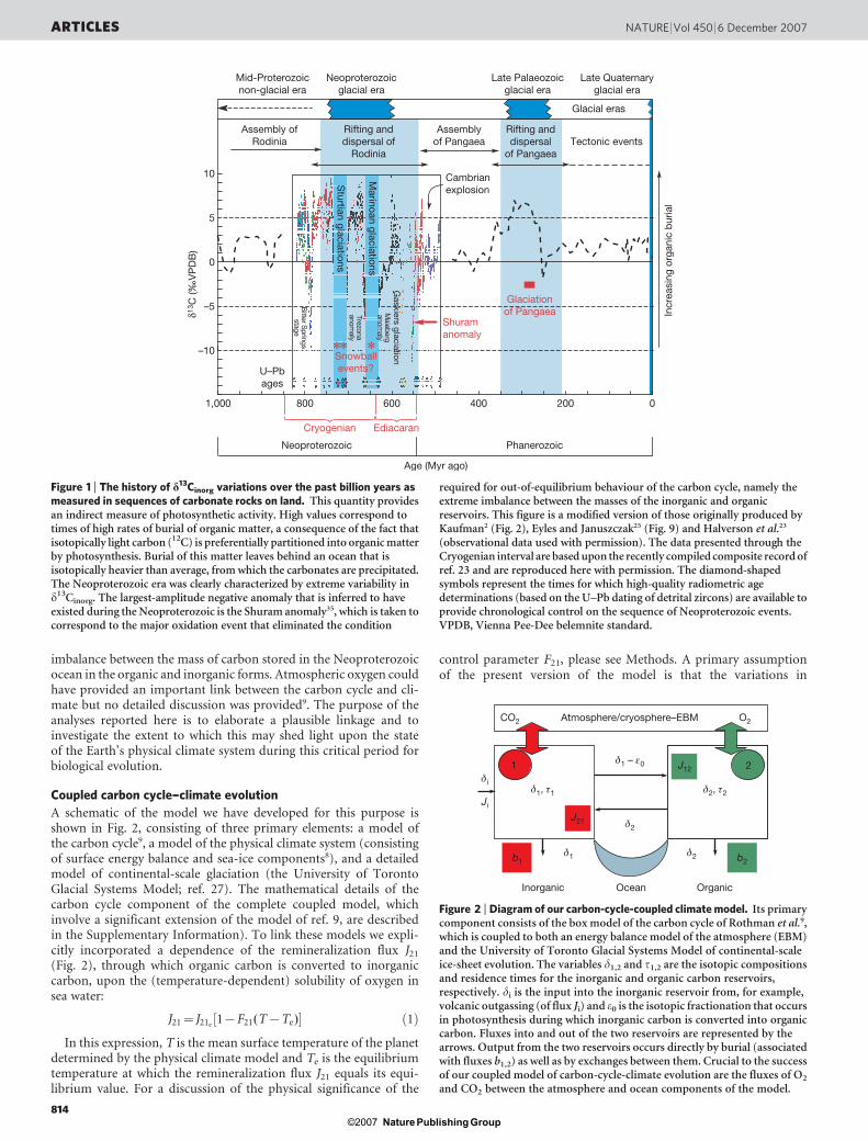
Figure 1 | The history of d13Cinorg variations over the past billion years asmeasured in sequences of carbonate rocks on land. This quantity providesan indirect measure of photosynthetic activity. High values correspond totimes of high rates of burial of organic matter, a consequence of the fact thatisotopically light carbon (12C) is preferentially partitioned into organic matterby photosynthesis. Burial of this matter leaves behind an ocean that isisotopically heavier than average, from which the carbonates are precipitated.The Neoproterozoic era was clearly characterized by extreme variability ind13Cinorg. The largest-amplitude negative anomaly that is inferred to haveexisted during the Neoproterozoic is the Shuram anomaly35, which is taken tocorrespond to the major oxidation event that eliminated the condition

required for out-of-equilibrium behaviour of the carbon cycle, namely theextreme imbalance between the masses of the inorganic and organicreservoirs. This figure is a modified version of those originally produced byKaufman2 (Fig. 2), Eyles and Januszczak25 (Fig. 9) and Halverson et al.23

(observational data used with permission). The data presented through theCryogenian interval are based upon the recently compiled composite record ofref. 23 and are reproduced here with permission. The diamond-shapedsymbols represent the times for which high-quality radiometric agedeterminations (based on the U–Pb dating of detrital zircons) are available toprovide chronological control on the sequence of Neoproterozoic events.VPDB, Vienna Pee-Dee belemnite standard.

1 2

δ2

δ2δ1

δ1 – ε0

δ2, τ2δ1, τ1

b1

J12

J21

Ji

δi

b2

CO2 O2Atmosphere/cryosphere–EBM

Inorganic Ocean Organic

Figure 2 | Diagram of our carbon-cycle-coupled climate model. Its primarycomponent consists of the box model of the carbon cycle of Rothman et al.9,which is coupled to both an energy balance model of the atmosphere (EBM)and the University of Toronto Glacial Systems Model of continental-scaleice-sheet evolution. The variables d1,2 and t1,2 are the isotopic compositionsand residence times for the inorganic and organic carbon reservoirs,respectively. di is the input into the inorganic reservoir from, for example,volcanic outgassing (of flux Ji) and e0 is the isotopic fractionation that occursin photosynthesis during which inorganic carbon is converted into organiccarbon. Fluxes into and out of the two reservoirs are represented by thearrows. Output from the two reservoirs occurs directly by burial (associatedwith fluxes b1,2) as well as by exchanges between them. Crucial to the successof our coupled model of carbon-cycle-climate evolution are the fluxes of O2

and CO2 between the atmosphere and ocean components of the model.

ARTICLES NATURE | Vol 450 | 6 December 2007

814Nature ©2007 Publishing Group

atmospheric oxygen that accompany system evolution will have nosignificant impact upon system dynamics.

The reason that the temperature dependence of the remineraliza-tion flux has important implications for the surface climate regime isconnected to the fact that as the climate cools and the rate of con-version of organic carbon to inorganic carbon increases, the partialpressure of carbon dioxide in the atmosphere also increases, accord-ing to the relation:

pCO2(t)

pCO2, e

~M1 tð ÞM1e

� �X

ð2Þ

in which pCO2, e 5 300 p.p.m.v. is the equilibrium concentration ofatmospheric carbon dioxide at temperature Te, M1 is the mass ofinorganic carbon in the ocean and M1e

is the equilibrium mass. Ithas been suggested28 that the parameter X in equation (2) should beequal to 2 in Phanerozoic circumstances in which the climate is notchanging too quickly. It is unclear whether the partition of carbondioxide between the ocean and the atmosphere during the rapidlychanging Neoproterozoic should obey this relationship, so we con-sider X to be a parameter of the model. As the level of atmospheric CO2

increases in response to increasing M1(t), the surface of the planet willbe increasingly heated by the increasing infrared flux of energy drad (inunits of W m22) that is due to ‘greenhouse’ warming29,30:

drad~6:0 lnpCO2

(t)

pCO2, e

� �ð3Þ

The sequence of relationships (1) to (3) together describe a nega-tive feedback process whereby the carbon cycle reacts to a tendency ofthe planet to cool by enhancing the atmospheric concentration ofcarbon dioxide and thus inhibiting the cooling. During warming thesame feedback operates so as to inhibit this tendency as well. The newcoupled model of carbon cycle–climate evolution that we havedeveloped for the Neoproterozoic is strongly controlled by this feed-back process.

Cyclic glaciation due to carbon cycle coupling

In the absence of explicit coupling to the carbon cycle, the ice-sheet-coupled energy-balance model of the process of global glaciation

produces steady-state solutions for the mean surface temperaturethat are a strong function of the concentration of carbon dioxidein the atmosphere, of the solar constant, and of the spatial distri-bution of the continents. Although the detailed palaeogeography ofthe Neoproterozoic varied appreciably during the break-up ofRodinia, there is general agreement that during the Sturtian epi-sode(s) the continental fragments were clustered around theEquator. During the Marinoan episode, however, the equatorialpositioning of the main land masses was apparently less pronounced.Here we use the same palaeogeography as was used in a previousanalysis7 of Neoproterozoic surface temperature conditions, one thatis more appropriate to the Marinoan glaciation than to theSturtian(s). For the value of the solar constant we assume a decreaseof 6% below the present value, as is appropriate to this stage of theevolution of the Sun.

In the absence of carbon cycle coupling, Fig. 3a shows the steady-state variations of mean surface temperature predicted by the ice-sheet-coupled EBM, as a function of atmospheric carbon dioxideconcentration. This model exhibits hysteresis, such that a range ofvalues of the parameter drad, and thus pCO2

, exists within which atleast two different steady states are equally acceptable solutions.Which state is physically realized depends upon the initial conditionsof integration from which the solution is approached, as indicated bythe arrows on the different branches of the diagram of steady-statesolutions. The hysteresis diagram defines a ‘hot branch’ of solutionsas well as an ‘oasis branch’, the latter being the branch on which the‘slushball’ solutions to the problem of Neoproterozoic climate wereoriginally discovered8. In this model the hard snowball solutionregime also exists, but to reach it requires that pCO2

(t) reaches suffi-ciently low values. To escape from the hard snowball state in thismodel requires approximately 0.3 bar of atmospheric carbon dioxideif the sea-ice albedo is assumed to be equal to 0.6 in the hard snowballregime7. This is somewhat lower than a more accurate estimate laterobtained with a more complex model31. Here we investigate how theclimate model will behave when coupled to the explicit model of thecarbon cycle.

The results delivered by this model in fully coupled synchronousmode are illustrated in Figs 3b–e, for which examples we haveassumed X 5 2 in equation (2). Figure 3b shows several cycles of

10

0

–10

–20

Hot branch

Oasis branch

T sur

f (°C

)T s

urf (

°C)

–12 –8 –4 0 4 ???drad (W m–2)

drad (W m–2)

Hard snowballHard snowball escape

048

–4–8

–8 –6 –4 –2 0 2 4Time in units of the period of

the glacial cycle, T

Land

ice

(106

km

3 )

0

200

400

600

a

b

b2b2b2

c

III

IV

III

100200

300

400500

pC

O2 (p

.p.m

.)

4060

80

100120

Sea

ice

(106

km

2 )

d

e

1T 2T 3T0

Figure 3 | The cyclic glaciation dynamics of the coupled climate–carboncycle model. a, The steady-state (equilibrium) solutions of the energy-balance-coupled ice-sheet model are shown as a function of the atmosphericcarbon dioxide concentration, represented by the increase or decrease of theinfrared flux, drad, received at the surface. The hysteresis in the model statespace is indicated by the multiple equilibria for a wide range of values of thecarbon dioxide concentration. b, The trajectory of solutions of the coupledclimate–carbon cycle model in the space of mean surface temperature versus

surface infrared forcing. The solution simply cycles the hysteresis loop of thesteady-state solutions when the impact of the temperature dependence of thesolubility of oxygen upon the remineralization flux is introduced into thedynamical system. c–e, Time series for sea-ice area, atmospheric carbondioxide concentration and land-ice volume are shown, respectively, forseveral circuits of the hysteresis loop. The scale of the x axis depends on thecontrol parameter F21, as demonstrated in Fig. 4.

NATURE | Vol 450 | 6 December 2007 ARTICLES

815Nature ©2007 Publishing Group

the ‘orbit’ of the solution in the plane of mean surface temperatureversus drad. These results demonstrate that the coupled systemevolves in such a way as to continuously cycle the hysteresis loopdefined by the set of steady-state solutions. In Figs 3c–e we show timeseries for sea-ice area, atmospheric CO2 and continental ice volumerespectively, for several circuits of the hysteresis loop. These resultsdemonstrate that system evolution is governed by a limit cycle oscil-lation (a periodic solution of the nonlinear dynamical system) whichwould have a period of approximately 4 Myr for F21 5 8 3 1025 anda period of approximately 30 Myr for F21 5 1 3 1025. Detailed ana-lysis (not shown) demonstrates that the onset of the periodic beha-viour for X 5 1 occurs for F21 , F21, crit, where the critical value is inthe range 5 3 1024 , F21, crit , 6 3 1024. For values less than this, theperiod of the limit cycle oscillation continues to increase as the valueof the control variable decreases. For X 5 2, the critical value of F21 isshifted to the range 3 3 1024 , F21, crit , 4 3 1024.

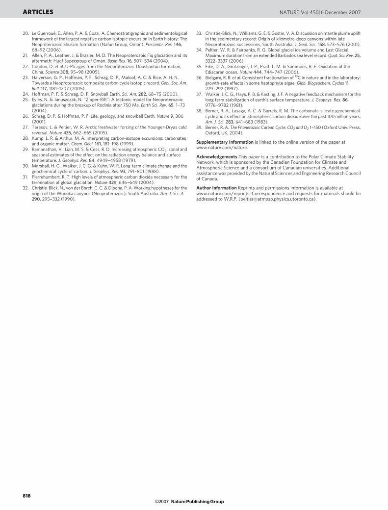
Figure 4, based upon analyses for several values of the control para-meter, for which time series are shown in Supplementary Fig. 1 (forX 5 1) and Supplementary Fig. 2 (for X 5 2), shows that the period ofthe limit cycle covers the previously inferred range of durations of theNeoproterozoic glacial intervals from 4 to ,30 Myr ago. In the limitF21R0, the previous model9 is recovered and the system exhibits nodynamics, as physical climate is now uncoupled from the carbon cycle.For F21 . F21, crit, the system exits the limit cycle regime (seeSupplementary Fig. 1 for F21 5 6 3 1024) and a new steady-state solu-tion is realized, one for which the mean surface temperature is equal tothe value Te (not shown). We interpret this ‘fixed point’ to representthe in-equilibrium solution for the carbon cycle that has apparentlybeen characteristic for the Phanerozoic eon that followed theNeoproterozoic with the onset of the Cambrian. The model thereforeembodies a potential explanation not only of the apparently out-of-equilibrium behaviour characteristic of the Neoproterozoic, but alsoof the in-equilibrium behaviour that has thereafter generally been therule9. Supplementary Fig. 3 shows normalized time series for all modelfields as a means of illustrating the phase relationships between them.

Eustatic sea level and ice volume variations

Figure 5 shows the distribution of land ice and sea ice over the surfaceof the Earth that the model delivers at each of the corners (labelled I toIV on Fig. 3a) of the hysteresis loop of steady solutions onto which thesolution is entrained in the time-dependent limit cycle regime. Thisregime is essentially perfectly periodic, so this set of four solutions fullycharacterizes the extremes of system behaviour. The low-temperature,

low-carbon dioxide corner of the loop (located at III in Fig. 3a) showsthat although most of the continental fragments are covered by a thickveneer of land ice and much of the surface of the ocean is covered by seaice, there is still a substantial area of the equatorial ocean that consistsof open water. This is the ‘slushball’ regime discovered previously8. Themaximum volume of land ice that develops during a single glacial cycleis approximately 500 3 106 km3, as shown on Fig. 3e, which wouldcorrespond to a fall of eustatic sea level of approximately 1 km, a resultthat could be interpreted as consistent with the deep Neoproterozoiccanyons that have been investigated on the Australian continent32,33.Although much larger, this sea-level depression is still reasonable com-pared to the sea-level drop of about 120 m that occurred during theLast Glacial Maximum34, when polar ice sheets covered only a smallfraction of the land surface.

We therefore interpret the Cryogenian period as a time duringwhich, in an organic-carbon-rich environment, the mass of organicmatter in the Neoproterozoic ocean had reached such a large valuerelative to the mass of inorganic carbon that out-of-equilibriumbehaviour with strong coupling to the physical climate systembecame possible. In our interpretation, this coupling ceased to bepossible after the intense oxidation of the organic reservoir thatoccurred towards the end of the Ediacaran period and just beforethe onset of the Cambrian22. We interpret this oxidation event ascoinciding with the Shuram anomaly shown on Fig. 135.

The isotopic variability of inorganic carbon

The model also predicts the time series of d13C(t) for the inorganicreservoir, the primary diagnostic that has been taken to require theexistence of the hard snowball regime. Escape from this regime isassumed to have been possible only via the build-up of the atmo-spheric carbon dioxide concentration owing to the presumed slowand continuous action of volcanic degassing while the oceans wereentirely covered by sea ice. To make contact with the different iso-topic concentrations of organic and inorganic carbon that developduring a single glacial cycle, the isotopic fractionation e0 that occursduring photosynthesis (see Fig. 2) must also depend upon oceanbiogeochemistry, and thus climate. To predict the evolution of car-bon isotopes we may therefore assume:

e0~eezbfrac, M(M1 CO2(t)½ �{M1e) ð4Þ

This representation of the isotopic fractionation that occurs dur-ing photosynthesis is intended to provide a parameterization of the

0 1 2 3 4 50

5

10

15

20

25

30

F21 (×10–4 °C–1)

Per

iod

of t

he g

laci

al c

ycle

, T (M

yr)

Figure 4 | The period of the glacial cycle predicted by the coupledclimate–carbon cycle model as a function of the control parameter of themodel F21. Results are shown for both X 5 1(solid line) and X 5 2 (dashedline), where X determines how the atmospheric carbon dioxide concentrationchanges as the mass of inorganic carbon changes relative to the referencevalues (equation (2)). The predicted period spans the range previouslyinferred to have been characteristic of Neoproterozoic glacial intervals.

II I

III IV

Land ice thickness (km)

0.5 1.5 2.5 3.5 4.5 5.5 6.5

Figure 5 | Examples of the distribution of land ice and sea ice during theglacial cycle. These examples correspond to the climate states occupied bythe model at each of the four corners (labelled I to IV) of the hysteresis loopof steady solutions shown on Fig. 3a. Irrespective of the value of the controlparameter, in the coupled mode the dynamical system simply continues tocycle the hysteresis loop. Land-ice thickness is contoured in shades of mauve,and sea ice is shown as white.

ARTICLES NATURE | Vol 450 | 6 December 2007

816Nature ©2007 Publishing Group

influence of kinetic isotope effects associated, say, with the enzyma-tically catalysed carboxylation of ribose bisphosphate (J. M. Hayes,personal communication, 2006). The mass of the inorganic reservoirM1 is expected to provide a reasonably direct representation of themain control on this catalytic process. This simple parameterizationappears to be in acceptable accord with the analyses of ref. 36 as usedin the discussion28 of the dependence of the isotopic differencebetween organic and inorganic carbon as a function of atmosphericpCO2

. Best fits of the model prediction of the time variation of d13C(t)through a typical Neoproterozoic glacial–interglacial cycle basedupon the use of equation (4) are obtained with a value of bfrac,M <0.00048% per gigaton. This value is not unreasonable given that thespecies composition of the hypothesized organic-carbon-heavyNeoproterozoic ocean, in which M2?M1, is largely unknown.

Figure 6a for X 5 2 shows the model prediction of the evolutionof d13Cinorg as a function of e 5 d1 2 d2, through a singleNeoproterozoic glacial–interglacial cycle, compared with the com-plete data set from ref. 9, inspection of which demonstrates the goodfit that the model is capable of delivering to the data. When thecomparison is limited to the interval of time from 738 to 593 Myrago that contains the Sturtian and Marinoan events (Fig. 6b), how-ever, the fit of the model to the data significantly improves. Thisdemonstrates that the carbon isotopic measurements from the inter-val containing the hypothesized hard snowball events are wellexplained by the carbon-cycle-coupled slushball model. As discussedin ref. 9, the slope of the model fit to the data in the d13Cinorg versus eplane is unity, which is highly diagnostic of the condition M2 ?M1

that is characteristic of the carbon cycle component of the model.Supplementary Fig. 4 shows equivalent results for the case X 5 1.

Future model developments

Among several further avenues of investigation as we continue todevelop this model of the coupled evolution of the carbon cycle andclimate during the Neoproterozoic, one we intend to explore concernsthe potential of the model as an explicit means of assessing the mag-nitude of the variations of atmospheric oxygen that would be expectedto accompany the glaciation–deglaciation process. Another concernswhether oxidants other than oxygen, such as sulphate, may have animportant role to play. Also, how might the drawdown of atmosphericcarbon dioxide from the atmosphere due to the weathering of calciumand magnesium silicates be expected to affect our model predictions16?Here we neglected this drawdown because of the strong temperatureand precipitation dependence that is characteristic of the silicateweathering process, such that low temperature and precipitationand the absence of vascular plants in this period of the Earth’s historywould have significantly reduced its effect37–39. In spite of this and otherremaining uncertainties, the new model strongly suggests that those

observations that have been assumed to be most diagnostic of hardsnowball conditions may not require such an extreme interpretation.In our view it is more likely that it may have been the carbon cycle, notthe physical climate system, that was operating in an extreme modebefore the onset of the Cambrian explosion of life.

METHODS SUMMARY

Our model consists of three primary components. (1) A global surface energy

balance model in spherical geometry with a specified distribution of continents

and ocean coupled to a simple thermodynamic model of sea-ice formation. This

element of the structure is time-dependent and may be subjected to orbital

insolation variations. It also resolves the annual cycle of surface temperature.

(2) A detailed model of the growth and evolution of continental ice sheets that

occurs in response to variations in the surface temperature and precipitation

regimes. In this model, precipitation forcing of the hydrological cycle is pre-

scribed. Furthermore, the glacial isostatic adjustment process that affects the

flow of ice over the surface of a continent under the action of the gravitational

force is fully incorporated. (3) A two-box model of the ocean carbon cycle that

differentiates between organic and inorganic reservoirs. Components (1) and (2)

are described in terms of coupled nonlinear partial differential equations

whereas the third component is described in terms of coupled nonlinear

ordinary differential equations. On the long timescales that are of interest to

us we may safely assume the concentration of carbon dioxide to be uniform

throughout the atmosphere at all times, because CO2 is a well-mixed atmo-

spheric trace gas. The three model components are coupled together throughthe action of an assumed temperature dependence of the remineralization flux

that converts organic carbon to its inorganic (CO2) form. The temperature

assumed to control the remineralization flux is taken to be the mean surface

temperature of the planet, a temperature that is dominated by the sea-surface

temperature of the tropical ocean.

Full Methods and any associated references are available in the online version ofthe paper at www.nature.com/nature.

Received 31 October 2006; accepted 1 October 2007.

1. Kirschvink, J. L. in The Proterozoic Biosphere: A Multi-Disciplinary Study (eds Schopf,J. W. & Klein, C.) 51–52 (Cambridge Univ. Press, Cambridge, UK, 1992).

2. Kaufman, A. J. An ice age in the tropics. Nature 386, 227–228 (1997).3. Hoffman, P. F., Kaufman, A. J., Halverson, G. P. & Schrag, D. P. A Neoproterozoic

Snowball Earth. Science 281, 1342–1346 (1998).4. Hoffman, P. F. & Schrag, D. P. The snowball Earth hypothesis: testing the limits of

global change. Terra Nova 14, 129–155 (2002).

5. Runnegar, B. Loophole for snowball Earth. Nature 405, 403–404 (2000).6. Knoll, A. H. Life on a Young Planet: The First Three Billion Years of Evolution on Earth

1–277 (Princeton Univ. Press, Princeton, New Jersey, 2003).7. Hyde, W. T., Crowley, T. J., Baum, S. K. & Peltier, W. R. Neoproterozoic ‘‘Snowball

Earth’’ simulations with a coupled climate/ice-sheet model. Nature 405,425–429 (2000).

8. Peltier, W. R., Tarasov, L., Vettoretti, G. & Solheim, L. P. in The Extreme Proterozoic:Geology, Geochemistry and Climate (eds Jenkins, G. S. et al.) Geophys. Monogr. Ser.,146, 107–124 (AGU Press, Washington DC, 2004).

9. Rothman, D. H., Hayes, J. M. & Summons, R. E. Dynamics of the Neoproterozoiccarbon cycle. Proc. Natl Acad. Sci. USA 100, 8124–8129 (2003).

10. Allen, P. A. Snowball Earth on trial. Eos 87, 495 (2006).11. Moczydlowska, M. Neoproterozoic and Cambrian successions deposited on the

east European platform and Cadomian basement area of Poland. Stud. Geophys.Geodaetica 39, 276–285 (1995).

12. Grey, K. & Corkoran, M. Late Neoproterozoic stromatolites in glacigenicsuccessions of the Kimberley region, Western Australia: evidence for a youngerMarinoan glaciation. Precambr. Res. 92, 65–87 (1998).

13. Chandler, M. A. & Sohl, L. E. Climate forcings and the initiation of low-latitude icesheets during the Neoproterozoic Varanger glacial interval. J. Geophys. Res. 105,20737–20756 (2000).

14. Goodman, J. C. & Pierrehumbert, R. T. Glacial flow of floating marine ice in‘‘Snowball Earth’’. J. Geophys. Res. 108, doi:10.1029/2002JC001471 (2003).

15. Poulsen, C. J. & Jacob, R. L. Factors that inhibit snowball Earth simulation.Paleoceanography 19, doi:10.1029/2004PA001056 (2004).

16. Donnadieu, Y., Godderis, Y., Ramstein, G., Nedelec, A. & Meert, J. A. ‘‘SnowballEarth’’ triggered by continental breakup through changes in runoff. Nature 428,303–306 (2004).

17. Pollard, D. & Kasting, J. F. Snowball Earth: a thin ice solution with flowing seaglaciers. J. Geophys. Res. 110, doi:10.1029/2004JC002525 (2005).

18. Pierrehumbert, R. T. Climate dynamics of a hard snowball Earth. J. Geophys. Res.110, doi:10.1029/2004JD0005162 (2005).

19. Leather, J., Allen, P. A., Brasier, M. D. & Cozzi, A. Neoproterozoic snowball Earthunder scrutiny: Evidence from the Fiq glaciation of Oman. Geology 30, 891–894(2002).

20 35

δ13 C

inor

g (‰

)

738–593 Myr ago738–593 Myr ago593–583 Myr ago583–555 Myr ago555–549 Myr ago

SturtianMarinoanNeither

8

6

4

2

0

–2

–4

δ13 C

inor

g (‰

)

8a b

6

4

2

0

–2

–425 30

ε (‰)20 3525 30

ε (‰)

Figure 6 | Model predictions of d13Cinorg(t) as a function of e(t) through asingle glacial cycle. These examples for the case X 5 2 are compared withobservations of contemporaneous samples of the isotopic ratios of organicand inorganic carbon at a large number of times through theNeoproterozoic. a, Comparison of all of the available data from Rothmanet al.9. b, The data derived from 738–593 Myr ago are shown separately andthe data points from the Sturtian and Marinoan intervals are singled out.

NATURE | Vol 450 | 6 December 2007 ARTICLES

817Nature ©2007 Publishing Group

20. Le Guerroue, E., Allen, P. A. & Cozzi, A. Chemostratigraphic and sedimentologicalframework of the largest negative carbon isotopic excursion in Earth history: TheNeoproterozoic Shuram formation (Nafun Group, Oman). Precambr. Res. 146,68–92 (2006).

21. Allen, P. A., Leather, J. & Brasier, M. D. The Neoproterozoic Fiq glaciation and itsaftermath: Huqf Supergroup of Oman. Basin Res. 16, 507–534 (2004).

22. Condon, D. et al. U-Pb ages from the Neoproterozoic Doushantuo formation,China. Science 308, 95–98 (2005).

23. Halverson, G. P., Hoffman, P. F., Schrag, D. P., Maloof, A. C. & Rice, A. H. N.Towards a Neoproterozoic composite carbon cycle isotopic record. Geol. Soc. Am.Bull. 117, 1181–1207 (2005).

24. Hoffman, P. F. & Schrag, D. P. Snowball Earth. Sci. Am. 282, 68–75 (2000).25. Eyles, N. & Januszczak, N. ‘‘Zipper-Rift’’: A tectonic model for Neoproterozoic

glaciations during the breakup of Rodinia after 750 Ma. Earth Sci. Rev. 65, 1–73(2004).

26. Schrag, D. P. & Hoffman, P. F. Life, geology, and snowball Earth. Nature 9, 306(2001).

27. Tarasov, L. & Peltier, W. R. Arctic freshwater forcing of the Younger-Dryas coldreversal. Nature 435, 662–665 (2005).

28. Kump, L. R. & Arthur, M. A. Interpreting carbon-isotope excursions: carbonatesand organic matter. Chem. Geol. 161, 181–198 (1999).

29. Ramanathan, V., Lian, M. S. & Cess, R. D. Increasing atmospheric CO2: zonal andseasonal estimates of the effect on the radiation energy balance and surfacetemperature. J. Geophys. Res. 84, 4949–4958 (1979).

30. Marshall, H. G., Walker, J. C. G. & Kuhn, W. R. Long-term climate change and thegeochemical cycle of carbon. J. Geophys. Res. 93, 791–801 (1988).

31. Pierrehumbert, R. T. High levels of atmospheric carbon dioxide necessary for thetermination of global glaciation. Nature 429, 646–649 (2004).

32. Christie-Blick, N., von der Borch, C. C. & Dibona, P. A. Working hypotheses for theorigin of the Wonoka canyons (Neoproterozoic), South Australia. Am. J. Sci. A290, 295–332 (1990).

33. Christie-Blick, N., Williams, G. E. & Gostin, V. A. Discussion on mantle plume upliftin the sedimentary record: Origin of kilometre-deep canyons within lateNeoproterozoic successions, South Australia. J. Geol. Soc. 158, 573–576 (2001).

34. Peltier, W. R. & Fairbanks, R. G. Global glacial ice volume and Last GlacialMaximum duration from an extended Barbados sea level record. Quat. Sci. Rev. 25,3322–3337 (2006).

35. Fike, D. A., Grotzinger, J. P., Pratt, L. M. & Summons, R. E. Oxidation of theEdiacaran ocean. Nature 444, 744–747 (2006).

36. Bidigare, R. R. et al. Consistent fractionation of 13C in nature and in the laboratory:growth-rate effects in some haptophyte algae. Glob. Biogeochem. Cycles 11,279–292 (1997).

37. Walker, J. C. G., Hays, P. B. & Kasting, J. F. A negative feedback mechanism for thelong term stabilization of earth’s surface temperature. J. Geophys. Res. 86,9776–9782 (1981).

38. Berner, R. A., Lasaga, A. C. & Garrels, R. M. The carbonate-silicate geochemicalcycle and its effect on atmospheric carbon dioxide over the past 100 million years.Am. J. Sci. 283, 641–683 (1983).

39. Berner, R. A. The Phanerozoic Carbon Cycle: CO2 and O2 1–150 (Oxford Univ. Press,Oxford, UK, 2004).

Supplementary Information is linked to the online version of the paper atwww.nature.com/nature.

Acknowledgements This paper is a contribution to the Polar Climate StabilityNetwork, which is sponsored by the Canadian Foundation for Climate andAtmospheric Science and a consortium of Canadian universities. Additionalassistance was provided by the Natural Sciences and Engineering Research Councilof Canada.

Author Information Reprints and permissions information is available atwww.nature.com/reprints. Correspondence and requests for materials should beaddressed to W.R.P. (peltier@atmosp.physics.utoronto.ca).

ARTICLES NATURE | Vol 450 | 6 December 2007

818Nature ©2007 Publishing Group

METHODS

By far the most important aspect of the coupled carbon cycle–climate model that

we have developed concerns the feedback between temperature and the rate at

which organic carbon is remineralized to produce inorganic carbon, as expressed

in equation (1). This relationship is supported by the well-known dependence,

through Henry’s law of classical thermodynamics, of the solubility of a gas in a

liquid upon the temperature of the liquid. Garcia et al.40 provide detailed

information on the basis of which we justify a linear parameterization of the

solubility of oxygen in sea water:

O2, sol~O2, sole {A(T{Te) ð5ÞThis dependence is introduced into the carbon cycle model by assuming that

the remineralization flux J21 is itself linearly dependent upon the deviation of the

solubility of oxygen away from its value at an equilibrium temperature Te. An

appropriate modification of the equilibrium flux J21ethat incorporates this

dependence (see Supplementary Information) is:

J21~J21e1zB

O2, sol{O2, sole

O2, sole

� �� �ð6Þ

Incorporation of equation (5) into equation (6) then gives equation (1) in the

main text.

The primary control parameter in the new coupled carbon cycle–climate

model is therefore the parameter F21, which has the dimensions of inverse

temperature:

F21~AB

O2, sole

ð7Þ

In the low-temperature vicinity of 1 uC, A < 8 mmol kg21 uC21 (ref. 40) and

O2, sol < 400mmol kg21 (ref. 40). Thus F21 < 3 3 1024uC21 for B 5 1.5 3 1022

(the importance of this value of F21 is discussed in the main text). The strength

of the dependence of the remineralization flux upon oxygen solubility that is

determined by the parameter B is clearly affected by ocean dynamics, including

the strength of the overturning circulation that operates under glacial condi-

tions. Although some model experiments have been performed8,41 in an attempt

to estimate this strength, and it is generally agreed that the thermohaline cir-

culation will act in such a way as to inhibit descent into the hard snowball state,

thermohaline circulation behaviour during the Neoproterozoic must be consid-

ered ill-constrained at present. This requires that a range of values for the para-

meter F21 be considered. Additional inhibition to snowball Earth formation in

the actual climate system may derive from the action of the wind-driven circula-

tion15 and the detailed characteristics related to sea-ice formation in the

tropics14,15 where incoming solar radiation is especially intense. Such additional

processes have been fully incorporated in a recently published simulation8 of

Neoproterozoic climate that has been preformed using the NCAR CSM 1.4

model.

The ‘two box model’ of the carbon cycle that is assumed to respond to climate

variability in the way described by the above relationships is coupled to a global

energy balance model (EBM) that is itself coupled to a thermodynamic sea-ice

module and a detailed model of continental-scale glaciation. The global EBM is

based upon that of North et al.42 as modified by Deblonde et al.43 to include a sea-

ice component. Because carbon dioxide is a well-mixed trace gas, when an

increase of the remineralization flux occurs as a consequence of decreasing

temperature and the resulting increase in carbon dioxide dissolved in the ocean

is partly partitioned into the atmosphere, there is no need to consider atmo-spheric variations in the spatial distribution of this greenhouse gas.

The model of continental-scale glaciation is based upon the use of the stand-

ard Glen flow law for the rheology and the shallow-ice approximation for the

dynamics. Because the topography of the Neoproterozoic continents is

unknown, the ice cover on the individual continental fragments is assumed to

develop on continental masses with a fixed initial freeboard of 400 m. As ice flows

from the land to the sea under the action of the gravitational force, calving is

assumed to act so as to eliminate ice beyond the continental termini. Processes

such as fast flow which are strongly conditioned by basal hydrology and sediment

deformation are eliminated from the model we employed. The isostatic adjust-

ment process that acts to modify the surface elevation of the ice sheet and thus

affects the surface mass balance is incorporated by assuming the process to act in

a simple damped return-to-equilibrium fashion with an assumed relaxation

time of 4,000 years, in acceptable accord with that appropriate for the Earth’s

present-day radial viscoelastic structure44. This is expected to be an excellent

approximation because, although the rheology of the planetary interior is

strongly temperature-dependent, the temperature of the interior has not chan-

ged significantly since Neoproterozoic time45.The climate forcing that is assumed to drive the advances and retreats of

both continental ice sheets and sea-ice cover is obtained from the surface tem-

perature field delivered by the EBM, assuming an annually averaged precipita-

tion rate of ,0.7 m yr21, which is appropriately diminished owing to the action

of the elevation desert effect, which acts so as to reduce the precipitation rate in

regions of high topographic relief such as for continents covered by substantial

thicknesses of glacial ice. These assumptions are the same as those previously

employed in the application of this model to the climate of the Neoproterozoic7.

The physical climate component of the carbon-cycle-coupled model has been

thoroughly exercised in a number of recent analyses of climate variations

through the Phanerozoic eon46,47 and in spite of its modest degree of complexity,

compared well against expectations based upon the GEOCARB model48 of past

variations in atmospheric carbon dioxide.

40. Garcia, H. E. & Gordon, L. I. Oxygen solubility in sea water: Better fitting equations.Limnol. Oceanogr. 37, 1307–1312 (1992).

41. Poulsen, C. J., Pierrehumbert, R. T. & Jacob, R. L. Impact of ocean dynamics on thesimulation of the Neoproterozoic ‘‘snowball Earth’’. Geophys. Res. Lett. 28,doi:10.1029/2000GL012058 (2001).

42. North, G. R., Mengel, J. G. & Short, D. A. Simple energy balance model resolvingthe seasons and continents: application to the astronomical theory of the ice ages.J. Geophys. Res. 88, 6576–6586 (1983).

43. Deblonde, G., Peltier, W. R. & Hyde, W. T. Simulations of continental ice sheetgrowth over the last glacial-interglacial cycle: experiments with a one levelseasonal energy balance model including seasonal ice albedo feedback. Glob.Planet. Change 98, 37–55 (1992).

44. Peltier, W. R. Postglacial variations in the level of the sea: implications for climatedynamics and solid-earth geophysics. Rev. Geophys. 36, 603–689 (1998).

45. Butler, S. L., Peltier, W. R. & Costin, S. O. Numerical models of the earth’s thermalhistory: Effects of inner core solidification and core potassium. Phys. Earth Planet.Inter. 152, 22–42 (2005).

46. Hyde, W. T., Crowley, T. J., Tarasov, L. & Peltier, W. R. The Pangean ice-age:Studies with a coupled climate-ice sheet model. Clim. Dyn. 15, 619–629 (1999).

47. Hyde, W. T., Grossman, E. L., Crowley, T. J., Pollard, D. & Scotese, C. R. Siberianglaciation as a constraint on Permian-Carboniferous CO2 levels. Geology 34,421–424 (2006).

48. Berner, R. A. GEOCARBSULF: A combined model for Phanerozoic atmospheric O2

and CO2. Geochim. Cosmochim. Acta 70, 5653–5664 (2006).

doi:10.1038/nature06354

Nature ©2007 Publishing Group

Snowball Earth prevention by dissolved organic carbon remineralization

W. Richard Peltier, Yonggang Liu & John W. Crowley

Supplementary Information

Since the global ice-sheet coupled energy balance model that is employed in coupled

carbon cycle mode in this paper has been well described in the existing literature, only a

cursory discussion of its properties will be presented herein. The sole extension to this

model beyond that described in Hyde et al.7 concerns the continental ice-sheet component

of this coupled structure. Whereas in Hyde et al.7 the version of the ice-sheet model

(ISM) employed was the isothermal version originally developed by Deblonde et al.30

,

the version employed for present purposes is the complete three dimensional thermo-

mechanically self consistent version of the model47

. This version of the ice-sheet model

has been subjected to detailed testing in the context of the European EISMINT

programme48

and is at the current state-of-the-art in this area of science. The most recent

application of this model has been to a detailed analysis of the history of freshwater

runoff from the North American continent during the transition from glacial to

interglacial conditions that began following Last Glacial Maximum approximately 21,000

years before present49

. The EBM to which this ice dynamics model is coupled includes an

enhancement of the original North et al.29

model by the addition of a thermodynamic sea-

ice module as discussed in Deblonde et al.30

. The model also includes a representation of

the glacial isostatic adjustment (GIA) process, a process that impacts ice sheet growth

and decay through the influence that topography has upon surface mass balance. For the

purpose of the analyses described in this paper, GIA effects are incorporated simply as a

damped return to equilibrium rather than by employing the more exact theory (e.g. as

reviewed in Peltier31

)

The carbon cycle model to which this EBM/ISM is coupled is based upon that

presented in Rothman et al.9. Since several properties of this model that were not

discussed in that paper are important for the purpose of the present application, the

mathematical details of the model and the modifications to it that have been made require

comment. The original box model is based upon that depicted in Figure 2, which

prominently represents the ocean component of the carbon cycle expressed as an

interaction between inorganic and organic reservoirs. The ordinary differential equations

required to describe this interaction are as follows:

( ) ( ) 0

1

1212

1

211

1

1 εδδδδδM

J

M

J

M

Ji

i +−+−=•

(S1)

( )201

2

122 δεδδ −−=

•

M

J (S2)

112211 bJJJMi

−−+=•

(S3)

SUPPLEMENTARY INFORMATION

doi: 10.1038/nature06354

www.nature.com/nature 1

221122 bJJM −−=•

(S4)

In the above equations the subscripted “J” and “b” quantities are mass fluxes that have

the dimensions of mass/unit time. The fluxes labeled “b” are burial fluxes that describe

the rate of deposition onto the ocean floor of material from the two carbon reservoirs.

The subscripted “δ” quantities represent the δ13C isotopic ratios of reservoirs “1” and “2”

and of the isotopic input into reservoir “1” due, for example, to volcanic degassing.

The model of the carbon cycle embodied in equations (S1-S4) has steady state

solutions, not catalogued in Rothman et al9, but which are important in the current

context. These steady state solutions may best be described in terms of the following

model dependent quantities. If we define by J1 and J2 the TOTAL mass fluxes into and

out of the inorganic and organic reservoirs respectively, then at equilibrium we must

have:

eeeeeJJbJJ

i 211121+=+= (S5)

eeeeJbJJ

122212=+= (S6)

in which the subscript “e” indicates an equilibrium value. The residence time constants

indicated on the box diagram in figure 2 of the paper are defined at steady state to be:

eeJM

111=τ , (S7)

eeJM

222=τ . (S8)

Additional quantities that are useful in representing the steady state solutions of the

Rothman et al.9 model are the normalized photosynthetic flux, φ12, the organic fraction of

the total burial flux, f, and the ratio of the residence times µ. These quantities have the

following definitions:

11212JJ=φ (S9)

( )212

bbbf += (S10)

21ττµ = (S11)

The above defined quantities may be usefully employed to define the steady state

solutions.

Detailed algebraic manipulation of the relations that follow from setting the left

hand sides of equations (S1)-(S4) to zero (not shown), lead to the following expressions

that define the steady states of the carbon cycle model. The critical quantity is the

normalized photosynthetic flux φ12 , the equilibrium value for which can be obtained by

substituting from equation (S5) into the definition (S9) to obtain, at equilibrium, that:

doi: 10.1038/nature06354 SUPPLEMENTARY INFORMATION

www.nature.com/nature 2

( )eeee

bJJ1121212

+=φ (S12)

In terms of the equilibrium mass of the inorganic carbon reservoir, M1, the mass of the

organic carbon reservoir at equilibrium turns out to be:

µ

φee

e

MM

112

2= , (S13)

whereas the equilibrium fluxes connecting the reservoirs to one-another and to the

external environment are the following:

( )( )f

MJ ee

ei −

−=

1

1

1

121

τ

φ (S14)

1

121

12τ

φee

e

MJ = (S15)

( )1

121

1

121

21

1

1 τ

φ

τ

φeeee

e

M

f

fMJ

−

−−= (S16)

It is equation (S16) for the re-mineralization flux that converts organic carbon back to the

inorganic form that is critical to the operation of the coupled climate-carbon cycle model

presented in this paper. Our assumption in designing this model is that the coupling

occurs primarily in an indirect way as a consequence of the strong temperature

dependence of the solubility of oxygen in sea water. As it is now well understood that the

planetary atmosphere had become rich in oxygen by approximately 2.3 Ga, by the time of

the Cryogenian period any occurrence of low surface temperatures that threatened to lead

to “hard snowball” surface glaciation would have led to a rapid draw down of oxygen

into the ocean as a consequence of Henry’s Law of classical thermodynamics. This would

have led to a strong increase in the rate of re-mineralization of the organic reservoir and

thus to an increase in dissolved inorganic carbon (DIC) and thus, in turn, to an increase of

carbon dioxide in the atmosphere and thus strong negative feedback upon the tendency of

the surface of the planet to further glaciate. This is the essence of the coupling that links

the carbon cycle to the greenhouse gas mediated surface climate regime. Because carbon

dioxide is a “well mixed” trace gas, the box model provides an adequate description of

the partitioning between the oceanic and atmospheric parts of the whole system inorganic

reservoir.

The set of nonlinear ordinary differential equations that replace the original

equations (S1)-(S4) of Rothman et al.9 are obtained by substitution of a surface

temperature modulated form of the equilibrium re-mineralization flux J21e and an

appropriate parameterization for the dependence upon climate of the photosynthetic

isotopic fractionation ε0. Otherwise the fluxes that mediate the interactions between the

reservoirs and the external environment are taken equal to their equilibrium values. The

set of ordinary differential equations that the procedure delivers is the following:

doi: 10.1038/nature06354 SUPPLEMENTARY INFORMATION

www.nature.com/nature 3

( ) ( ) [ ]( ) [ ]( )efraceei

iMM

M

JTTF

M

J

M

Jeee

11

1

12

2112

1

21

1

1

1 1 −++−−−+−=•

βεδδδδδ (S17)

[ ]( ))( 1121

2

122 efrace MM

M

Je −+−−=

•

βεδδδ (S18)

)(21211 eTTJFMe

−−=•

(S19)

)(21212

eTTJFM

e−+=

•

(S20)

The model is then completely described by specifying values for the quantities φ12e, µ, τ1,

εe, δi, βfrac, Te and f. The values selected for these parameters for the calculations reported

in this paper are essentially identical to those employed in the paper by Rothman et al.9

and are respectively 0.999, .01, 1000 years, 28 per mil, -6 per mil, variable, 1 degree

Celsius, and 0.3. As in the paper by Rothman et al.9 the selected values for φ12e and µ

result in an organic reservoir mass that is approximately 100 times the mass of the

inorganic reservoir. The initial mass of the inorganic carbon reservoir does not affect the

dynamics in any way, but in our calculations has been initialized to the value of 40,000

Giga tons estimated by Kump et al.50

to be the amount of inorganic carbon present in the

modern ocean. The temperature employed for the purpose of coupling the carbon cycle to

the model of the physical climate system is taken to be the mean surface temperature for

the purpose of the analyses presented in this paper.

Although space has allowed only a single example of the characteristics of solutions

to the coupled climate carbon cycle model to be displayed in the main body of the paper,

it will be of interest to some readers to see specific examples of the dependence of the

time scale of the limit cycle oscillation that the model delivers upon the magnitude of the

control parameter F21. This dependence is illustrated in Figures S1 and S2 in which we

show a set of simulated time series of continental ice volume for a range of F21 values

with the value of the parameter “X” (see equ. (2)), that controls the partition of carbon

dioxide between the ocean and the atmosphere, set to the value 1 and 2 respectively. A

graph of the dependence of the period of the limit cycle oscillation upon this control

variable is shown as Figure 4 in the main body of the paper for both X=1 and X=2. It will

be clear on the basis of these results that episodes of glaciation with durations of order a

few million years are easily accommodated by the model. Even the period of ~70 million

years separating the Sturtian and Marinoan events could be accommodated if this were

considered to be the fundamental glacial period since the period diverges to very large

values in the limit that F21→0. This demonstrates that, as a consequence of carbon cycle

coupling, “slushball” modes of deep glaciation are easily able to satisfy the claim by

Schrag and Hoffman25

that the geological record requires that episodes of Neoproterozoic

glaciation have durations of at least 4 Ma. Figure S3 presents a sequence of amplitude

doi: 10.1038/nature06354 SUPPLEMENTARY INFORMATION

www.nature.com/nature 4

normalized time series, with the mean removed, for each of the primary field variables of

the model. This presentation makes possible an inter-comparison of phase relationships

between these characteristics of the model thorugh a number of glacial cycles.

In order to demonstrate that our ability to fit the observed Neoproterozoic variations

of the difference between the carbon isotopic ratios of inorganic and organic carbon is not

restricted to the case X=2, Figure S4 shows the fit for the case X=1 for which a different

value of the parameter βfrac = 0.00028, rather than the value employed for the case X=2

which was 0.00048 and for which results were shown on Figure 6 in the main body of the

paper. The simple linear approximation for the dependence of the photosynthetic isotopic

fractionation upon the mass of the inorganic carbon reservoir that we are employing for

the purpose of the results presented in this paper is very easily accommodated within the

more detailed biogeochemical description provided by the model of Kump and Arthur36

.

This simply requires appropriate changes in the constants of their model, constants that

were originally derived by fitting to data from the Phanerozoic. Since the Neoproterozoic

system differed dramatically from its Phanerozoic counterpart, the requirement for some

adjustment of the parameters of their model is required for application to the

Neoproterozoic is understandable.

Supplementary References

47. Tarasov, L. & Peltier, W.R. Impact of thermo-mechanical ice sheet coupling on a model of the 100 kyr

ice age cycle. J. Geophys. Res. 104, 9517-9545 (1999).

48. Payne, A.J. et al. Results from the EISMINT model inter-comparison: the effects of thermo-

mechanical coupling. J. Glaciology 46, 227-238 (2000).

49. Tarasov, L. & Peltier, W.R. A calibrated deglacial drainage chronology for the North American

continent: Evidence of an Arctic trigger for the Younger-Dryas. Quat. Sci. Rev. 25, 659-688 (2006).

50. Kump, L.R., Kasting, J.F. & Crane, R.G. The Earth System. Pearson Education Inc. Upper Saddle

River, New Jersey (2004), 419pp.

doi: 10.1038/nature06354 SUPPLEMENTARY INFORMATION

www.nature.com/nature 5

Figure S1 Time series of continental ice volume for a range of F21 values, for the

model employing linear dependence (namely X=1 in equ. (2)) of pCO2 on the mass

of dissolved inorganic carbon. The solid lines are directly from the model

calculation, whereas the dashed extensions to each of the time series are

extrapolations on the basis of the demonstrated periodicity to enable each of the time

series to cover the same range of time.

doi: 10.1038/nature06354 SUPPLEMENTARY INFORMATION

www.nature.com/nature 6

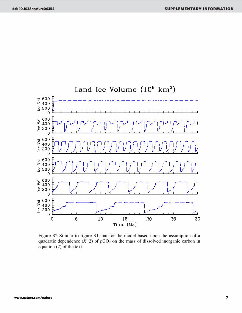
Figure S2 Similar to figure S1, but for the model based upon the assumption of a

quadratic dependence (X=2) of pCO2 on the mass of dissolved inorganic carbon in

equation (2) of the text.

doi: 10.1038/nature06354 SUPPLEMENTARY INFORMATION

www.nature.com/nature 7

Figure S3 Amplitude normalized time series, with the mean removed, are shown for

several ice age cycles and for 6 different field variables of the model. These include the

variation in the infrared radiative forcing at the surface of the Earth, the mean surface

temperature, land ice volume, the masses of the inorganic and organic carbon reservoirs

and sea ice area.

doi: 10.1038/nature06354 SUPPLEMENTARY INFORMATION

www.nature.com/nature 8

Figure S4 This representation of the dependence of inorgC13δ upon ε is similar to

figure 6 in the main body of the paper except that this is for the model with the

control parameter “X” set equal to 1.

doi: 10.1038/nature06354 SUPPLEMENTARY INFORMATION

www.nature.com/nature 9

factors in V. cholerae. But this idea raises possi-ble public-health issues: the activation of quo-rum sensing in V. cholerae also induces active movement of the bacterium, potentially mobi-lizing the pathogen and encouraging the spread of infection from one person to another.

For several years, the repertoire of bacte-rial quorum-sensing signal molecules and receptors was thought to be rather limited and restricted to a few species. But recent studies have revealed an array of different signals, suggesting that we have only just scratched the surface of possible mechanisms. As new signals are identified and their use by bacteria is assessed, the list of quorum-sensing organisms will undoubtedly grow. We may

eventually reach a point at which bacteria that do not engage in quorum sensing are regarded as the exception, rather than the norm. The challenge now is not only to identify new sys-tems, but also to make sense of why an organism would use one type of system over another. ■

Matthew R. Parsek is in the Department of Microbiology, University of Washington, Box 357242, Seattle, Washington 98195-7242, USA.e-mail: parsem@u.washington.edu

1. Miller, M. B., Skorupski, K., Lenz, D. H., Taylor, R. K. & Bassler, B. L. Cell 110, 303–314 (2002).

2. Zhu, J. et al. Proc. Natl Acad. Sci. USA 99, 3129–3134 (2002).3. Camilli, A. & Bassler, B. L. Science 311, 1113–1116 (2006).4. Higgins, D. A. et al. Nature 450, 883–886 (2007).5. Sperandio, V. Expert Rev. Anti-infect. Ther. 5, 271–276

(2007).

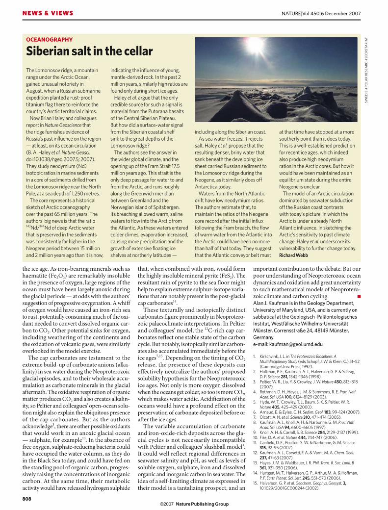
PALAEOCLIMATE

Slush findAlan J. Kaufman

A coupled model of palaeoclimate and carbon cycling turns up the heat on the idea that Earth once became a giant snowball. It supports instead a milder ‘slushball Earth’ history — but piquant questions remain.

Sediments laid down in the oceans during the late Neoproterozoic era, between about 850 million and 542 million years ago, tell a dramatic story. They contain wildly varying abundances of the carbon isotope 12C, which is typically incorporated into organic matter dur-ing photosynthesis. The pattern of excess 12C in carbonates immediately above and below gla-cial deposits seems to indicate that photosyn-thesis on Earth came to a halt during a series of ice ages. These observations are a foundation of the ‘snowball Earth’ hypothesis1,2: that, just before the first appearance of animals, Earth’s surface might have been repeatedly frozen over, even at tropical latitudes.

Not necessarily so, say Peltier et al. on page 813 of this issue3. They apply basic ideas about the solubility of gases to a coupled model of climate and carbon cycling4 during the frigid late Neoproterozoic era. The results that emerge might explain the oscillatory carbon-isotope compositions of carbonates across the Neoproterozoic glacial cycles, without resort-ing to the hard-snowball model. Instead, they could lend support to a milder variation on the same theme — ‘slushball Earth’.

The slushball and snowball models both predict ice sheets on continents near the Equa-tor, but with markedly different extents of ice covering the oceans. In the snowball version, the frozen planet is completely blanketed, and reflects most of the Sun’s warming rays back into space. Temperatures plummet and surface processes, including life, largely cease. Escape from the snowball state probably requires the build-up of volcanic carbon dioxide in the atmosphere over many millions of years,

resulting in torrential acid rain and the intense weathering of exposed rocks during the global thaw.

The slushball model5, by contrast, predicts open glacial oceans that would have con-strained runaway refrigeration by allowing sunlight to warm the planet’s surface, driving an active hydrological cycle6 and photosyn-thesis7 in exposed seas. The end of such an ice age need not have required extreme amounts of CO2 in the atmosphere, nor have been delayed for millions of years.

Peltier and colleagues’ new dynamic model3 shows how climate and atmospheric oxygen might have combined to prevent a runaway snowball Earth. As the oceans cool during ice ages, lower temperatures allow atmospheric gases such as oxygen to diffuse more read-ily into the deep sea, forcing the oxidation of abundant dissolved organic carbon, formed initially by photosynthesis in surface waters, to CO2. Released back to the atmosphere by this oceanic ‘respiratory’ process, the excess CO2 would warm the planet and thereby end the glacial epoch.

What is particularly interesting about this model is that climate drives the carbon cycle (and so determines the stable levels of atmos-pheric CO2). In the most recent ice ages, as well as for earlier interpretations of Neoproterozoic carbon-isotope anomalies8, the assumption has instead been the other way around. The crucial difference is that the Neoproterozoic carbon cycle was conceivably buffered by a marine pool of dissolved organic carbon that was orders of magnitude larger than that in the present-day oceans4.

A pertinent criticism of Peltier and col-leagues’ mathematical model is the uncer-tainty in its input parameters, in particular the assumption that levels of atmospheric oxygen were similar to those of today (around 21%). Biological9 and geochemical10–12 evidence indi-cates that oxygen levels were low throughout most of the Neoproterozoic, with a significant rise in breathable air around 550 million years ago — about the time animals first appeared on the planet. In that case, it seems likely that pervasive oxygenation of the atmosphere and the hydrosphere, including the vast pool of dissolved organic carbon, occurred millions of years after the extensive ice sheets of the Neoproterozoic had melted away. This rise, known as the Wonoka anomaly after the local-ity in South Australia in whose rocks it was first observed, is recorded in 550-million-year-old carbonates worldwide that are spectacularly rich in 12C.

The coupled model also does not address certain hallmark geological features of the Neoproterozoic glacial episodes. These include the unexpected appearance of iron-bearing sediments in the glacial deposits, as well as the enigmatic ‘cap carbonates’ that lie immediately above them (Fig. 1). The co-occurrence of iron-oxide cements and glacial sediments implies that levels of soluble iron increased during

Figure 1 | A soluble solution? The large (5–8-cm high) carbonate crystal fans (black to dark grey), which seem to grow out of the sea floor in this polished slab of a Neoproterozoic ‘cap carbonate’ from Brazil, suggest the presence of high concentrations of dissolved inorganic carbon in sea water after the ice ages, together with the rapid accumulation of sediments. These fans are draped by grey to white, fine-grained carbonates, which near the top become red, probably because they contain the iron-oxide mineral haematite (Fe2O3). The isotopic composition of such geological deposits is a focus of Peltier and colleagues’ model interpretation3 of Neoproterozoic climate and carbon cycling.

A. J

. KA

UFM

AN

807

NATURE|Vol 450|6 December 2007 NEWS & VIEWS

the ice age. As iron-bearing minerals such as haematite (Fe2O3) are remarkably insoluble in the presence of oxygen, large regions of the ocean must have been largely anoxic during the glacial periods — at odds with the authors’ suggestion of progressive oxygenation. A whiff of oxygen would have caused an iron-rich sea to rust, potentially consuming much of the oxi-dant needed to convert dissolved organic car-bon to CO2. Other potential sinks for oxygen, including weathering of the continents and the oxidation of volcanic gases, were similarly overlooked in the model exercise.

The cap carbonates are testament to the extreme build-up of carbonate anions (alka-linity) in sea water during the Neoproterozoic glacial episodes, and to their wholesale accu-mulation as carbonate minerals in the glacial aftermath. The oxidative respiration of organic matter produces CO2 and also creates alkalin-ity, so Peltier and colleagues’ open-ocean solu-tion might also explain the ubiquitous presence of the cap carbonates. But as the authors acknowledge3, there are other possible oxidants that would work in an anoxic glacial ocean — sulphate, for example13. In the absence of free oxygen, sulphate-reducing bacteria could have occupied the water column, as they do in the Black Sea today, and could have fed on the standing pool of organic carbon, progres-sively raising the concentrations of inorganic carbon. At the same time, their metabolic activity would have released hydrogen sulphide

that, when combined with iron, would form the highly insoluble mineral pyrite (FeS2). The resultant rain of pyrite to the sea floor might help to explain extreme sulphur-isotope varia-tions that are notably present in the post-glacial cap carbonates14.

These texturally and isotopically distinct carbonates figure prominently in Neoprotero-zoic palaeoclimate interpretations. In Peltier and colleagues’ model, the 12C-rich cap car-bonates reflect one stable state of the carbon cycle. But notably, isotopically similar carbon-ates also accumulated immediately before the ice ages7,15. Depending on the timing of CO2 release, the presence of these deposits can effectively neutralize the authors’ proposed solubility hypothesis for the Neoproterozoic ice ages. Not only is more oxygen dissolved when the oceans get colder, so too is more CO2, which makes water acidic. Acidification of the oceans would have a profound effect on the preservation of carbonate deposited before or after the ice ages.

The variable accumulation of carbonate and iron-oxide-rich deposits across the gla-cial cycles is not necessarily incompatible with Peltier and colleagues’ slushball model3. It could well reflect regional differences in seawater salinity and pH, as well as levels of soluble oxygen, sulphate, iron and dissolved organic and inorganic carbon in sea water. The idea of a self-limiting climate as expressed in their model is a tantalizing prospect, and an

important contribution to the debate. But our poor understanding of Neoproterozoic ocean dynamics and oxidation add great uncertainty to such mathematical models of Neoprotero-zoic climate and carbon cycling. ■ Alan J. Kaufman is in the Geology Department, University of Maryland, USA, and is currently on sabbatical at the Geologisch–Paläontologisches Institut, Westfälische Wilhelms-Universität Münster, Corrensstraße 24, 48149 Münster, Germany.e-mail: kaufman@geol.umd.edu

1. Kirschvink, J. L. in The Proterozoic Biosphere: A Multidisciplinary Study (eds Schopf, J. W. & Klein, C.) 51–52 (Cambridge Univ. Press, 1992).

2. Hoffman, P. F., Kaufman, A. J., Halverson, G. P. & Schrag, D. P. Science 281, 1342–1346 (1998).

3. Peltier, W. R., Liu, Y. & Crowley, J. W. Nature 450, 813–818 (2007).

4. Rothman, D. H., Hayes, J. M. & Summons, R. E. Proc. Natl Acad. Sci. USA 100, 8124–8129 (2003).

5. Hyde, W. T., Crowley, T. J., Baum, S. K. & Peltier, W. R. Nature 405, 425–429 (2000).

6. Arnaud, E. & Eyles, C. H. Sedim. Geol. 183, 99–124 (2007).7. Olcott, A. N. et al. Science 310, 471–474 (2005).8. Kaufman, A. J., Knoll, A. H. & Narbonne, G. M. Proc. Natl

Acad. Sci. USA 94, 6600–6605 (1997).9. Knoll, A. H. & Carroll, S. B. Science 284, 2129–2137 (1999).10. Fike, D. A. et al. Nature 444, 744–747 (2006).11. Canfield, D. E., Poulton, S. W. & Narbonne, G. M. Science

315, 92–95 (2007).12. Kaufman, A. J., Corsetti, F. A. & Varni, M. A. Chem. Geol.

237, 47–63 (2007).13. Hayes, J. M. & Waldbauer, J. R. Phil. Trans. R. Soc. Lond. B

361, 931–950 (2006).14. Hurtgen, M. T., Halverson, G. P., Arthur, M. A. & Hoffman,

P. F. Earth Planet. Sci. Lett. 245, 551–570 (2006). 15. Halverson, G. P. et al. Geochem. Geophys. Geosyst. 3,

10.1029/2001GC000244 (2002).

The Lomonosov ridge, a mountain range under the Arctic Ocean, gained unusual notoriety in August, when a Russian submarine expedition planted a rust-proof titanium flag there to reinforce the country’s Arctic territorial claims.

Now Brian Haley and colleagues report in Nature Geoscience that the ridge furnishes evidence of Russia’s past influence on the region — at least, on its ocean circulation (B. A. Haley et al. Nature Geosci. doi:10.1038/ngeo.2007.5; 2007). They study neodymium (Nd) isotopic ratios in marine sediments in a core of sediments drilled from the Lomonosov ridge near the North Pole, at a sea depth of 1,250 metres.

The core represents a historical sketch of Arctic oceanography over the past 65 million years. The authors’ big news is that the ratio 143Nd/144Nd of deep Arctic water that is preserved in the sediments was consistently far higher in the Neogene period between 15 million and 2 million years ago than it is now,

indicating the influence of young, mantle-derived rock. In the past 2 million years, similarly high ratios are found only during short ice ages.

Haley et al. argue that the only credible source for such a signal is material from the Putorana basalts of the Central Siberian Plateau. But how did a surface-water signal from the Siberian coastal shelf sink to the great depths of the Lomonosov ridge?

The authors see the answer in the wider global climate, and the opening up of the Fram Strait 17.5 million years ago. This strait is the only deep passage for water to and from the Arctic, and runs roughly along the Greenwich meridian between Greenland and the Norwegian island of Spitsbergen. Its breaching allowed warm, saline waters to flow into the Arctic from the Atlantic. As these waters entered colder climes, evaporation increased, causing more precipitation and the growth of extensive floating ice shelves at northerly latitudes —

including along the Siberian coast.As sea water freezes, it rejects

salt. Haley et al. propose that the resulting denser, briny water that sank beneath the developing ice sheet carried Russian sediment to the Lomosonov ridge during the Neogene, as it similarly does off Antarctica today.

Waters from the North Atlantic drift have low neodymium ratios. The authors estimate that, to maintain the ratios of the Neogene core record after the initial influx following the Fram breach, the flow of warm water from the Atlantic into the Arctic could have been no more than half of that today. They suggest that the Atlantic conveyor belt must

at that time have stopped at a more southerly point than it does today. This is a well-established prediction for recent ice ages, which indeed also produce high neodymium ratios in the Arctic cores. But how it would have been maintained as an equilibrium state during the entire Neogene is unclear.

The model of an Arctic circulation dominated by seawater subduction off the Russian coast contrasts with today’s picture, in which the Arctic is under a steady North Atlantic influence. In sketching the Arctic’s sensitivity to past climate change, Haley et al. underscore its vulnerability to further change today.Richard Webb

OCEANOGRAPHY

Siberian salt in the cellar

SWED

ISH

PO

LAR

RESE

ARC

H S

ECRE

TARI

AT

808

NATURE|Vol 450|6 December 2007NEWS & VIEWS