6 Data Analysis Techniques for Human Microwire …scholar.harvard.edu/files/kreimanlab/files/rutishauser_ch06.pdfestimates of the relationships between extracellular waveform amplitudes

PROPERTY OF MIT PRESS: FOR PROOFREADING AND INDEXING PURPOSES ONLY

Fried—Single Neuron Studies of the Human Brain

R

Data Acquisition and Processing

This chapter gives a technical perspective on the procedures for an experiment to proceed from the acquisition of continuously sampled data from microwires all the way to points of time a putative single neuron fired a spike, to local field potential (LFP) recordings, and to decoding neurophysiological signals in single trials and in real time.

In order to analyze extracellular waveforms, it is important to acquire data with high sampling rates. Sampling rates below 16 kHz can miss important aspects of the submillisecond structure of action potential waveforms. Current systems typically have sampling rates above 30 kHz. Another methodological consideration involves the use of 60 Hz notch filters. While purists will advocate examining raw data without any filters, the clinical environment often presents signifi-cant challenges and electrical artifact contaminations for neurophysiological recordings. Remov-ing 60 Hz and harmonics with a notch filter can significantly enhance the signal-to-noise ratio (SNR) to discriminate action potentials. The focus in this chapter starts at the point of time the data has been stored by the acquisition system whereas chapter 5 in this volume describes the acquisition system and electrodes themselves.

Microwires record the extracellular voltage at a particular point in space. This signal, a voltage as a function of time, is the linear superposition of a great number of current sources generated by electrically active components of the brain (Buzsáki et al., 2012), including syn-aptic events and action potentials propagating down an axon or backpropagating inside den-drites. In general, it is extremely difficult to decompose the extracellular signal into the single events that give rise to it. An important aspect of the extracellular signals that can sometimes lead to a reasonable interpretation is the occurrence of action potentials in the near vicinity of the microwire tip. In the rat hippocampus CA1 region, it has been estimated that electrodes can distinguish extracellular spikes from neuronal processes located as far away as 140 μm from the tip of the electrode (Buzsáki, 2004). The peak amplitude depends on the physical size of the neurons under study, making it most likely that a majority of extracellular record-ings involve pyramidal cells (Henze et al., 2000) (see also brief discussion of extracellular waveforms in chapter 8). To our knowledge, in human recordings, there are no quantitative

6 Data Analysis Techniques for Human Microwire Recordings: Spike Detection and Sorting, Decoding, Relation between Neurons and Local Field Potentials

Ueli Rutishauser, Moran Cerf, and Gabriel Kreiman



R


60 Ueli Rutishauser, Moran Cerf, and Gabriel Kreiman

estimates of the relationships between extracellular waveform amplitudes and shapes and neu-ronal types or distances to neighboring neurons. However, since the peak amplitude of extra-cellular spikes decreases rapidly as a function of distance and cell sizes are roughly comparable in rodents and humans, it is reasonable to assume that the basic properties of extracellular recordings summarized in Buzsáki et al. (2012) are also applicable in human neurophysiology. Thus, if action potential sources occur sufficiently close to the microwire and the sources are sparse in space and time, the extracellular signal can distinguish the shapes of the single waveforms sufficiently well to allow a clustering process that groups waveforms of sufficient similarity into clusters that originate from putative single neurons. Animal studies with move-able electrodes (such as implanted microdrives) allow experimenters to move the electrode in small steps to optimize the position till the waveforms show the desired properties (waveform, amplitude, number of clusters). This procedure is often followed in intraoperative recordings in humans, particularly during the implantation of deep brain stimulation devices in humans (see chapters 15–16). In contrast, during semi-chronic recordings in epileptic patients, microw-ires are implanted under anatomical guidance without simultaneous recordings and without moving the microwires to optimize the recordings.

For the reasons outlined above, the variety of extracellular waveforms encountered is large. In practice the question frequently arises as to whether a particular waveform could possibly be neuronal or rather some sort of artifact. To gain intuition into what kinds of waveforms can be obtained from extracellular recordings, it is instructive to consult computational studies simulat-ing voltage in the extracellular milieu of reconstructed neurons from which both intra- and extracellular potentials were recorded simultaneously (Harris et al., 2000; Gold et al., 2006). These studies show that the extracellular waveform originating from a single neuron varies greatly as a function of the relative position of the electrode with respect to the neuron. Apart from the amplitude, other features that change systematically include the width, the number of peaks, as well as the sign (positive or negative) of the waveform (see figure 2 in Gold et al., 2006). The extracellular waveform results because of three different currents that flow in and out of cells: Na+ inflow, K+ outflow, and capacitive current. The different components are visible to different extents at different locations in the cell, which explains the great variability of waveforms. For example, positive-going waveforms can result from the capacitive current in distal dendrites. Usually, the simultaneously occurring Na+ current masks the capacitive current, but in distal dendrites the Na+ current is delayed. This results in bipolar or reverse-polarity waveforms. Situations where waveforms of different cells appear with different polarity on the same wire are thus possible. In our experience, this happens routinely in human recordings from the human medial temporal lobe. Another aspect that influences the shape of extracellular wave-forms is the incidence of bursting. Subsequent spikes within a bust typically show distinct waveform properties. The discussion so far has focused on the extracellular waveform obtained from considering a single neuron. In actual recordings, the microwires capture the activity of multiple neurons and neighboring neurons can also affect the shape of the extracellular

PROPERTY OF MIT PRESS: FOR PROOFREADING AND INDEXING PURPOSES ONLY PROPERTY OF MIT PRESS: FOR PROOFREADING AND INDEXING PURPOSES ONLY


R

Data Analysis Techniques for Human Microwire Recordings 61

waveform. In particular, simultaneous (or nearly simultaneous) action potentials from nearby neurons can lead to action potential waveforms that do not resemble each individual waveform (but could perhaps be modeled as a linear superposition of such individual waveforms).

In addition to spike sorting to separate different units contributing to the extracellular record-ing, the shape of the extracellular waveform can be used to infer tentative information about the morphology and type of the neuron recorded from. For example, the width of the waveform can be used to distinguish between inhibitory and excitatory neurons, which has been done also in humans (Viskontas et al., 2007) (see also chapter 8). Also, there are significant correlations between the peak amplitude, spike width, and electrode distance that can be used to infer mor-phological features as well as the approximate electrode location (Gold et al., 2006). However, for such inferences to be accurate, the waveform has to be preserved as authentically as possible. This requires using software and hardware filters which do not distort the waveform. For example, filters that are used to discard the low-frequency components of the extracellular signal can greatly distort waveforms (Quiroga, 2009; Wiltschko et al., 2008). The distortions are caused by filters that have a phase lag that is a function of frequency, such as causal Butterworth filters (Quiroga, 2009). As a precaution, little or no filtering (if feasible) should be done in hardware, and all software filters should have zero-phase lag (which are noncausal). Also, real-time spike detection and sorting by necessity are based on causal filtering, which means that the waveforms produced by such methods are greatly distorted. It is thus advisable to post hoc redo all spike detection and sorting offline from the broadband signal. Another source of potential artificial waveforms is band-pass-filtered artifacts. Band-pass filtering almost any high-frequency signal (such as a static discharge) will result in a waveform which looks approximately like a spike. Therefore, great care has to be taken to distinguish between artifacts and neuronal spikes. One such approach is to use independent metrics such as statistics based on the distribution of inter-spike intervals (ISIs).

Spike Detection and Sorting

The first steps after continuously sampled raw signals have been acquired (see figure 6.1A, plate 1) are to (1) detect the spikes and (2) identify which putative neuron the spikes originated from (“spike sorting”). Inferring the number of putative neurons contributing to a collection of wave-forms is an ill-posed inverse problem with no unique or “best” solution due to the sparseness of the available data. Recording the same spike simultaneously from multiple spatial locations greatly increases the ability to distinguish different neurons with similar waveforms. This can be achieved with tetrodes or silicon probes, but these techniques are not yet widely available for human recordings, and we thus focus on single wire recordings.

Various algorithms and procedures have been developed for manual, semi-automatic, or fully automatic spike sorting, and a number of software packages are available either as open source or commercially. These approaches have been reviewed and compared in the literature (Lewicki,



R



0

100

0

40

Am

p [µ

V]

0

10

20

0 0.2 0.4 0.6 0.8 1.0 1.2 1.4 1.6 1.8

0

40

Time [sec]

Am

p [µ

V]

Am

p [µ

V]

Am

p [a

u]

−200

20406080

0 20 40 600

1

2

3

Frequency [Hz]

(Spk

/s)^

2

0 200 400 600

10

Time [ms]

Am

plitu

de [µ

V]

0 20 40 60

1

2

3

Frequency [Hz]

0 200 400 600

10

Time [ms]

0 20 40 60

2

4

6

Frequency [Hz]

0 200 400 600

10

Time [ms]

0 10 200

0.2

0.4d=20

−5 0 5 10 15 200

0.2

0.4d=11

−5 0 5 10 150

0.2

0.4d=9

Time [ms]0.5 1.0 1.5

Time [ms]0.5 1.0 1.5

Time [ms]0.5 1.0 1.5

Num

ber

of s

pike

s

Distance [x s.d.]

Pro

babi

lity

Pro

babi

lity

Pro

babi

lity

A)

B) C)

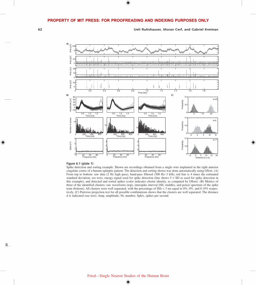
Figure 6.1 (plate 1)Spike detection and sorting example. Shown are recordings obtained from a single wire implanted in the right anterior cingulate cortex of a human epileptic patient. The detection and sorting shown was done automatically using OSort. (A) From top to bottom: raw data (2 Hz high pass), band-pass filtered (300 Hz–3 kHz; red line is 4 times the estimated standard deviation; see text), energy-signal used for spike detection (line shows 5 × SD as used for spike detection in this example), and detected and sorted spikes (color indicates cluster identity, as computed by OSort). (B) Metrics of three of the identified clusters: raw waveforms (top), interspike interval (ISI; middle), and power spectrum of the spike train (bottom). All clusters were well separated, with the percentage of ISIs < 3 ms equal to 0%, 0%, and 0.19% respec-tively. (C) Pairwise projection test for all possible combinations shows that the clusters are well separated. The distance d is indicated (see text). Amp, amplitude; Nr, number; Spk/s, spikes per second.



R


1998; Pouzat et al., 2002; Quiroga et al., 2004; Rutishauser et al., 2006; Gibson et al., 2012). Procedures developed for animal models are generally applicable also for humans, but there are several aspects unique to human recordings that deserve discussion.

Spike DetectionThe first step in the process of spike sorting is the identification of individual spikes and their waveforms (see figure 6.1A, plate 1). There is a critical dependency between sorting and detec-tion: Better detection makes sorting easier. Detection involves several steps: (1) determining the point of time a spike occurred, (2) determining the waveform of this spike, and (3) realigning this waveform to a common reference frame that makes it comparable to all other collected waveforms. Here, we will highlight a few types of detection approaches that have been applied to human recordings.

Amplitude thresholding methods are the simplest: A spike is detected if the band-pass filtered raw signals (e.g., >300 Hz) crosses a predefined threshold such as a multiple of the standard deviation of the underlying signal. A threshold that is frequently used is

T n medianx=

0 6748.,

where n is a constant (typically n = 4) and the second term is an estimate of the standard devia-tion of the noise in the voltage x (Donoho & Johnstone, 1994; Quiroga et al., 2004). An example of this threshold is shown in figure 6.1A (plate 1). Note that this method requires the user to choose a direction of spiking (positive, negative, or both). This choice is often performed manu-ally on a channel-by-channel basis. If spikes are prominent in both directions, special care has to be taken to ensure the same spike is not detected twice as many waveforms have approximately equal amplitude in both directions.

More sophisticated spike detection methods rely on a derivate signal, which is then thresh-olded in a similar manner to amplitude thresholding. Such derivative signals have the advantage that their SNR can be higher due to selective amplification, a standard approach in signal pro-cessing (Kay, 1993). An example is an energy-type model that estimates the likelihood of a spike’s being present as a function of time (Bankman et al., 1993; Kim and Kim, 2003). A method frequently used in human recordings (Rutishauser et al., 2006, 2008; Rutishauser et al., 2010) as well animal recordings (Csicsvari et al., 1998) is the following: Convolve the band-pass-filtered raw signal with a rectangular kernel that has the approximate width of a spike, that is, 1 ms (but note that for some recordings, this value will have to be adjusted accordingly depending on the neuron type, such as when recording dopaminergic neurons as in Zaghloul et al., 2009). The rectangular kernel is a matched filter that will amplify signals of appropriate width and suppress spike-like waveforms of widths that are smaller or larger. This can be com-puted very efficiently using a convolution kernel (see Appendix A.1. in Rutishauser et al., 2006, for implementation details). The resulting signal is strictly positive and can be thresholded at a multiple of its own standard deviation (typically in the range of 3.5–6 × SD). An example of



R



this method is shown in figure 6.1A (plate 1) with a threshold of T = 5. There are other, more sophisticated, methods that compute a multiscale version of the energy signal (Choi et al., 2006) which are promising but have, to our knowledge, not been evaluated rigorously for use with human recordings.

A third class of detection methods that has been used is wavelet based. This is typically computationally more expensive but can lead to improved detection performance particularly in low SNR recordings (Nenadic & Burdick, 2005). There are well-studied wavelets such as the bior family, which resemble the waveforms of spikes and thus yield better detection compared to the simple rectangular kernel used by energy-signal methods.

Choosing an appropriate spike-detection method is based on carefully weighting several trade-offs, such as detection performance, computational cost and complexity, implementation com-plexity, real time versus offline performance, and for some applications power requirements. Investing more in detection makes sorting easier whereas investing more in sorting allows simpler detection methods. Our experience indicates that it pays to understand the behavior of the particular method used in detail by building intuition using simulated data or data recorded simultaneously intra- and extracellularly (Obeid, 2007). Only such data sets allow the rigorous determination of false-positive and true-positive rates as well as sweeps of thresholds to build detection receiver operating characteristic (ROC) curves (see figure 8 in Nenadic & Burdick, 2005, for an example). Performing an ROC-based performance evaluation using data sets simu-lated to resemble SNR ranges and waveform shapes in a particular data set can greatly improve the understanding of the parameters and trade-offs of a particular method.

A crucial step that follows detection is spike alignment. This can be an error-prone step, which can lead to substantial sorting quality problems or spurious clusters. Most sorting methods are based on distance metrics that assume that a common point of the waveform is at a fixed loca-tion in the matrix that holds all the detected waveforms. Common alignment points are the peak, trough, half-max amplitude, or the point of maximal slope. However, consistently identifying this point in waveforms is difficult. Note that the alignment point will typically be different from the point of threshold crossing, which shows considerable variability. Many waveforms are biphasic and have approximately equal amplitudes in both directions (on average). In such situ-ations, using the location with the maximal absolute amplitude will lead to the creation of two clusters. This is because, due to variability, for some spikes the peak will be maximal whereas for others the trough will show a larger amplitude. A common solution to this problem is twofold: Either the peak or trough is always used, or a preference is enforced in which always the first significant (with respect to background noise) peak or trough is used as the alignment point (Rutishauser et al., 2006). The first case works well if spikes are dominant in one direction, which is often case. However, this requires a manual choice of alignment for each channel (usually by visual inspection). This is because in the bipolar recordings often used for chroni-cally implanted microwires in humans, the direction of the spikes is arbitrary, depending on where the ground wire is located. An additional difficulty to consider is that the location of the peak is very sensitive to the sampling rate. Since the time spent at the peak is minimal, it is



R


unlikely that the recording sampled the exact peak location. The probability of sampling the true peak increases with the sampling rate. For example, the peak location of a typical spike has less than 0.2 ms uncertainty, which for a sampling rate of 30 kHz is represented by eight data points. The accuracy of peak finding can be increased by upsampling the signal to a higher sampling rate (such as 100 kHz) before peak finding.

Spike SortingThe goal of spike sorting is to assign each detected waveform to a putative single neuron that generated this spike (see figure 6.1A, plate 1, bottom). The number of possible unique neurons that could be present in a recording is unknown and also has to be estimated—that is, spike sorting is an unsupervised clustering problem where the number of the clusters is unknown. There are many unsupervised clustering approaches, and a number of such methods have been applied to spike sorting. These methods are reviewed extensively elsewhere (Lewicki, 1998; Pouzat et al., 2002; Quiroga et al., 2004; Rutishauser et al., 2006; Gibson et al., 2012). Rather than describe specific algorithms, we will review different spike-sorting approaches and discuss general issues that we found of relevance in our human recordings work.

Human recordings from semi-chronically implanted microwires are unique in that the microw-ires are not movable. Also, under most circumstances, no recordings take place during implanta-tion, so microwire location cannot be optimized with respect to yield and signal quality. In contrast, electrode position can usually be optimized specifically for unit yield in animal models. In addition, experiment time with awake behaving humans is very limited. Thus, only a limited number of spikes is available for any given neuron, making spike sorting more difficult. Addi-tionally, neurons in the brain areas typically covered by implanted electrodes tend to have very small baseline firing rates and sparse response properties. This further increases the demands on spike sorting as, in extreme cases, neurons might only respond to a few trials out of a long experiment (e.g., chapter 8). Not only will such neurons yield only a few spikes, but it is not possible to predict a priori what aspects of the task will elicit activity in those neurons. Detailed study of such neurons will thus require an adaptive experiment that shows stimuli which are chosen such that they are relevant for the neurons that are currently being recorded. This presents the challenge of requiring rapid spike sorting. Some experiments may also call for online sorting in order to achieve real-time decoding capacity (see this chapter and also chapter 17). Neces-sarily, such quick spike sorting, whether on- or offline, has to be semi- or fully automated. One criterion to consider is thus speed of sorting and possibilities to automate the process. Different approaches exist, starting with fully manual “cluster cutting” or window discriminators, semi-automatic cluster cutting where manual user interaction serves to refine automatic clustering, and automatic sorting either online or offline. Manual postprocessing is required even with so-called “fully automatic” spike-sorting approaches. This includes deciding between types of clusters, such as those that likely represent single units, those that are multiunits, and others that are noise. Clusters that represent noise should not be discarded but rather identified as such because these clusters will attract the noise spikes and prevent them from becoming intermingled



R



with other clusters. Often, manual processing also includes deciding that some identified clusters have to be merged because they are too similar.

Examples of software packages and their mode of operation that have been used for human recordings are as follows:

1. MClust—manual; A.D. Redish et al.2. KlustaKwik—semi-automatic with manual refinement (Harris et al., 2000)3. OSort—automatic online sorting, manual cluster (Rutishauser et al., 2006)4. Wave_clus—automatic offline sorting, manual cluster selection (Quiroga et al., 2004).

In addition, several commercial equipment manufacturers now offer integrated online spike detection and sorting. While these algorithms are necessarily less sophisticated, they can be good enough for quick online sorting during the experiment or to drive stimulus selection; however, offline reanalysis is usually required for more fine-grained analyses.

In addition to speed and accuracy, an important consideration in spike sorting is consistency. While some decisions made during this process are necessarily subjective, one would at least like to have these decisions always be made in a consistent, well-understood manner. Automatic spike sorting ensures this if it is combined with a systematic manner of implementing the manual postprocessing steps. This is of great importance to get consistent and comparable results across experimenters in a lab and, hopefully, across labs.

As with spike detection, it is important to understand and have an intuition for the spike-sorting approach utilized. Such an intuition can be built by using a data set of simulated neural recordings that is representative of the recording situation. Benchmark data sets of different difficulty levels are available for this purpose—for example, as part of OSort or Wave_clus (see above for references). These should be used to systematically evaluate the performance of spike sorting in terms of clusters identified, false positive/true positive/missed spikes.

Quality MetricsDue to the uncertainty and subjectivity inherent in spike sorting, appropriate quantitative metrics should be applied and reported to allow comparisons between studies, groups, and investigators. For example, what exact definitions were used to classify a unit as “single unit” as opposed to “multiunit”? The exact parameters vary to some degree and are subjective, which requires that the definitions be consistent, quantitative, and clearly reported. Such metrics can be classified into two groups: (1) single unit measures and (2) comparisons between different units. The first includes metrics such as the mean waveform, its variance, and its SNR; properties of the ISI such as the proportion of ISIs below some minimal threshold or its distribution; or the autocor-relation of spike times. The second includes metrics to quantify the difference between two or more putative single units—for example, by using pairwise distance metrics (see below). Such metrics are instrumental in establishing consistent criteria to evaluate whether two units are distinct and whether such distinction remains stable over time.



R


The SNR of a spike quantifies to what extend the waveform is different from the “back-ground.” A common definition of the SNR is the root mean square of the individual or average waveform over some period of time (such as 2.5 ms), divided by the standard deviation of the noise (estimated from segments where no spikes were detected; Bankman et al., 1993). The SNR is positively correlated with the waveform amplitude and negatively correlated with the ampli-tude of the background noise. It is useful to compute the SNR for each individual waveform and then quantify the variance of the SNR for all spikes associated to a given cluster. Similarly, the SNR of the waveforms can be plotted as a function of time to evaluate the stability of the unit and its isolation over time. Generally, the higher the SNR of a set of waveforms, the higher the likelihood that a well-isolated single unit can be discriminated.

Typically, a collection of spikes that potentially originated from a single neuron is identified based entirely on the properties of the waveform (such as its shape, SNR, energy) alone. If this is the case, the points of time at which these spikes occurred is a statistically independent metric that can be used to evaluate the sorting result. Metrics that are useful for this purpose are either based on the ISI distribution or on the autocorrelation of the spike times. Due to the refractory period of neurons, very short ISIs (<3 ms) are highly unlikely and should therefore be rare in a well-isolated unit. A useful metric is thus the proportion of ISIs shorter than a few milliseconds apart (see figure 6.1B, plate 1, for an example). For example, in one study, we found that the average ISIs < 3 ms for all isolated units was 0.3% (Rutishauser et al., 2008) . The refractory period also leads to a “dip” in the autocorrelation function of the spike train, which can be used to derive a similar test (Gabbiani & Koch, 1999). The autocorrelation and power spectrum of spike trains (figure 6.1B, plate 1, shows examples) is very sensitive to deduce whether a unit contains artificial spikes caused by highly regular sources such as line noise (leading to peaks at 16.6 ms for 60 Hz) or refresh-triggered noise of CRT or LCD screens (up to 240 Hz). In our experience, a combination of at least these three metrics is necessary to confidently declare a cluster to be a single unit. For example, a noise-corrupted unit can well have 0% ISIs below 3 ms and high SNR.

A second class of metrics serves to quantify how well a unit is separated from other isolated or unidentified units. Whether two or more units are truly distinct or not can be difficult to determine based on the waveforms alone, particularly because of the challenges in visualizing high-dimensional spaces. Statistical methods can be used both to help the sorting process itself and to quantify and document the results (Schmitzer-Torbert et al., 2005; Joshua et al., 2007; Hill et al., 2011). One metric that has been applied to human single unit data is the projection test (Pouzat et al., 2002). It is based on the observation that, given a particular level of back-ground noise, two units need to be separated by a minimal distance to be statistically different. If the waveforms of two units are more similar than this minimal distance, they cannot be dif-ferentiated given the present noise level. This does not mean that the two units are not different but that they cannot be distinguished reliably given the recording conditions and thus have to be considered the same. The projection test is a pairwise metric that, for each pair of units, defines their distance as a multiple of this minimally distinguishable distance. The properties of



R



the background noise are calculated from spike-free segments of the recording—that is, after all detected spikes have been removed. The background (neuronal and noise) in extracellular record-ings typically has a significant negative or positive autocorrelation for periods of up to several milliseconds. For example, in one human data set the autocorrelation function was found to be significant up to 1.2 ms (figure 3 in Rutishauser et al., 2006). This means that the noise is col-ored—that is, the noise amplitude at successive data points is not independent. This violates the “white-noise” assumption of many statistical tests. The technique of “whitening” a signal, a standard tool in signal processing (Kay, 1993), removes correlated noise to make signals white. This reveals the actual waveforms without artificial smoothening due to correlated noise.

The projection test consists of the following steps: (1) estimation of the noise autocorrelation, (2) prewhitening of detected spikes and normalization of the standard deviation of the noise, (3) pairwise calculation of distance between two clusters. The distance between two clusters is the distance between the two mean waveforms at the center of the two clusters. It is strictly positive and is expressed in units of multiples of the standard deviation of the point around the cluster center. For example, a distance of 5 means that the two cluster centers are separated by 5 standard deviations whereas the points around each center have standard deviation 1 (by definition after the normalization). We recommend this metric as very convenient both for setting rigorous criteria for what minimal distances are acceptable and for documenting the population of neurons constituting a given study (figure 6.1C, plate 1, shows examples). For example, in one study (Rutishauser et al., 2008) we found that the mean pairwise distance between all possible pairs of units recorded on the same wire was 13.7 in units of standard deviations. A histogram of these pairwise distances is a convenient way to summarize the separation criteria of a study (see figure S12 in Rutishauser et al., 2008, for an example).

To what degree are the results of a particular study dependent on spike sorting? It will depend greatly on the experimental measure under investigation whether a result will depend greatly on separation criteria or not. To evaluate such concerns rigorously, it is useful to calculate the metric of interest (such as a response or selectivity index) for all neurons recorded followed by rank ordering the results according to spike-sorting/isolation metrics such as the SNR, the percentage of short ISIs (ISIs within the refractory period could reflect poor sorting), or the projection test distance. If there is a significant correlation between the metric under investigation and the quality metric, further steps have to be taken to avoid confounds. For example, the threshold for inclusion of neurons could be set appropriately based on examination of these correlations with isolation and recording quality (Schmitzer-Torbert et al., 2005).

The Relation between Spikes and the LFP

Signal AcquisitionThe spikes originating from a single neuron are a local measure of neuronal spiking output. However, neurons are embedded in a multitude of networks. They receive inputs from and project to a large number of other neurons and can thus hardly be considered independent. Depending



R


on brain state and the area and the unit recorded from, some neurons fire in synchrony with many others whereas in other instances their firing appears to be mostly independent of others. This changing extent of synchrony of firing relative to other neurons is of great interest for investigating phenomena such as functional connectivity, plasticity, and many aspects of cogni-tion such as top-down attention. One approach to quantify such dependencies is to evaluate to what extent the spiking of a particular neuron correlates with aspects of the LFP recorded from the same or a different microelectrode.

Several different types of signals are often referred to as “LFPs.” While investigators have used the term LFP to discuss scalp electroencephalographic recordings or intracranial recordings (sometimes referred to as “electrocorticography,” or “ECoG”), those signals are less “local” than the ones we consider here. Here we focus on the low-pass band of the extracellular recordings from microwire electrodes. A critical variable that influences how local the field potentials are is the impedance of the electrode. We suggest restricting the term LFP to signals recorded from high-impedance (>100 kΩ) microwire electrodes. Typically, the low-pass corner frequency may be set at 100 Hz. Depending on the type of analyses, the exact corner frequency may be relevant since higher frequencies show a significant contribution from spiking activity in the same elec-trode (Logothetis, 2002; Zanos et al., 2011; Buzsáki et al., 2012). While there continues to be significant debate about how local LFPs really are (and the answer likely depends on the elec-trode diameter, impedance, recording area, relevant frequencies, and other variables), several studies have suggested that LFPs capture activity within a radius of a few hundred micrometers in the vicinity of the electrode (Buzsáki et al., 2012).

If spikes and LFPs are recorded from the same electrodes, it is necessary to consider whether the waveforms of the spikes could possibly “leak” into the LFP frequencies of interest and thus introduce artificial phase locking. Simulations indicate that this can be the case for frequencies above 50 Hz (Logothetis, 2002; Zanos et al., 2011; Buzsáki et al., 2012). For purposes of analysis of the LFP with respect to phase locking, such leakage of power into low frequencies is unde-sired. To prevent this, it is necessary to replace the samples around a detected spike such that the spike is removed from the LFP. This can be achieved by replacing spikes with a cubic spline interpolation between 1 ms before and 2 ms after the peak of the spike (in the high-resolution signal at full sampling rates). More sophisticated methods for spike removal have also been suggested (Zanos et al., 2011).

Of particular interest here is whether the probability of spiking correlates systematically with the power and/or phase of a specific oscillatory component (such as theta frequency oscillations) of the LFP. Other types of relationships have also been investigated, such as broadband power increases and their relationship to single unit firing (Miller et al., 2007; Manning et al., 2009). There are several methods for quantifying the spike–field relationship, of which we highlight two: direct estimation based on instantaneous power/phase and indirect estimation using spike–field coherence (SFC).

All methods require that the low-frequency (LFP) and high-frequency (spikes) parts of the signal are available simultaneously. This means that, if a spike occurs at t = 100.0 ms, we need



R



to know the power and phase of the oscillations that are part of the LFP at this exact moment in time. While this might seem trivial, in reality this is sometimes not the case because of frequency-dependent time lags introduced by components of the acquisition system, the elec-trode, or the data processing pipeline. Such artifacts have to be corrected for, as otherwise they produce artificial spike–field relationships because systematic shifts that have a different (but fixed) lag as a function of frequency will make them appear systematically before/after the spike whereas in reality these two happened simultaneously. In practice, there are three principle sources of such artifacts: (1) filters used by the data acquisition system, (2) the head stage, and (3) filters in the postacquisition data processing.

Filters used by the data acquisition system are typically causal (as they are applied in real time), which means they have a phase lag dependent on frequency (as discussed above). Fre-quently, experimenters have the acquisition system apply two types of filters: LFP band (such as 0.5–100 Hz) and spikes (such as 300–3000 Hz). The system then processes and stores each component independently, such as in a continuous data file and in a file with detected spikes. In such a situation careful analysis is necessary to ensure that the filters used for the two bands have the same phase-lag response (which typically they do not). Some systems display the time lag introduced (which can reach several milliseconds) and allow switching on a correction mode. We advise avoiding this situation altogether by saving the data in as broadband a format as pos-sible and then extracting spikes and the LFP from the very same file using noncausal zero-phase lag filters.

The second possible source of signal distortions is the head stage. Careful modeling and analysis studies have demonstrated that head stages with too low input impedances distort the LFP to such an extent that artificial spike–field correlations are induced and/or the spike wave-forms are significantly distorted (Nelson et al., 2008; Nelson & Pouget, 2010). This can be avoided by using head stages with input impedances > 1 GΩ. This is necessary because of the relatively high impedance of the electrodes, typically in the range of 400 kΩ–1 MΩ. Some of the commercial head stages frequently used for human recordings are well characterized and have sufficiently high input impedances. One example is the HS-36 electrode we used in a recent study (Rutishauser et al., 2010) which has >1 TΩ input impedance. However, there are many other systems being used that have either unknown or too low input impedance for this type of recording. In such situations, manual corrections by deconvolution can be applied as has been done by some authors (Siegel et al., 2009), and some suppliers offer tools to achieve this (i.e., FPAlign by Plexon Inc.). An additional area of concern is filtering done directly in the head stage. The hardware filters in the head stage have to be known or experimentally measured to ensure that they do not introduce phase shifts in the range of interest. Such shifts can easily reach 90° for low frequencies (Nelson et al., 2008), meaning the measured signal will lead the actual signal by one fourth of the cycle length. This can lead to misinterpretations or null results that are due to these phase-distortion artifacts. The effective impedance of the head stage is reduced by the cabling between the head stage input and the electrode through capacitive coupling (Robinson, 1968), providing a further incentive to make these cables as short as possible.



R


Quantitative MeasuresThe aim of measures to quantify the relationship between spikes and the LFP is to quantify statistically whether the spike times of a particular neuron are related to the phase and/or power of an oscillatory component of the LFP. In this section, we focus on phase relationships, but similar methods can be applied for power. We summarize two methods: assessing phase locking using circular statistics and SFC.

Circular Statistics and Estimation of Instantaneous Phase Circular statistics provide a method to assess the distribution of circular variables such as phase angles (Fisher, 1993). Examples are circular equivalents of the normal distribution (the von Mises distribution) and circular tests for uniform distribution of variables (the Rayleigh test, among many others). In the following we quantify phases θ in units of radians in the range of – ,π …, π where θ = 0 is the peak and θ = ±π is the trough (see figure 6.2). This notation is used in many analysis programs such as MATLAB.

Figure 6.2Illustration of the notation for phases. Shown are 1.5 cycles of an oscillation (arbitrary units). The corresponding angle is shown in the bottom two rows both in radians (rad; middle) and degrees (deg; bottom). In this notation, the peak of the oscillation corresponds to 0° and the trough to ±180°. Note the discontinuity at 180°, when the phase resets.



R



The free MATLAB toolbox CircStat contains implementations of many statistical tests and tools necessary for the analysis of circular data (Berens, 2009).

Applying circular statistical tools first requires that the phase of the underlying oscillation(s) be determined for every point of time where a spike occurred. There are many ways to achieve this, of which we outline two common methods that have been employed successfully to analyze human single neurons and their relationship to the LFP (Caplan et al., 2001; Jacobs et al., 2007; Rutishauser et al., 2010): (1) the Hilbert transform and (2) the wavelet transform (see also Le Van Quyen et al., 2001, for a comparison of these two methods). The Hilbert transform is par-ticularly useful when there is a certain frequency of interest (such as 35 Hz) whereas wavelet methods are more natural when a range of frequencies is considered.

After the phases for all spikes fired by a neuron have been determined (see below), the next step is to determine whether the population of phase values θi is distributed significantly around their mean angle θ or whether their distribution is, alternatively, uniform and thus random. The mean resultant vector R is the vector sum of all the phase angles:

C ii l

n

= ( )=∑cos θ , S i

i l

n

= ( )=∑sin θ , R C S2 2 2= + , R

R

n= . (6.1)

In the above, C and S are the normalized sums of the sine and cosine of each phase angle, respectively, and n represents the total number of phase angles. The larger the length of the mean resultant R (range 0…1), the stronger the phase locking of the neuron is. The sample circular variance is V R= −1 . To test whether a neuron is significantly phase locked, the sample of all phase angles was compared against uniformity using a Rayleigh test. The Rayleigh test is based on a statistic Z:

Z nR= 2, P ZZ Z

n

Z Z Z

n= −( ) + − − − + −

exp 12

4

24 132 76 9

288

2 2 3 4

2

Ζ. (6.2)

If P is sufficiently small, the null hypothesis of uniformity can be rejected. The alternative hypothesis is that the data are unimodal (one mean direction). Notice that the Rayleigh test is strictly a function of R as well as of n (number of spikes included). The same value of R thus leads to different significance values depending on the number of spikes that are included. In practice this leads to the problem that, given enough spikes, neurons that are not convincingly phase locked lead to statistical significance at P < 0.05. It is worthwhile to estimate a reasonable p-value cutoff for the numbers of spikes considered using simulations. Frequently, studies use cutoffs of P < 0.01 or P < 0.001 to avoid false positives. Due to these problems, we have found it advantageous to use summary metrics other than R and the Rayleigh-test significance value. These are based on the von Mises distribution, the circular equivalent of the normal distribution (Fisher, 1993):

fI

θπ κ

κ θ µ( ) = ( )−( )( )1

2 0

exp cos . (6.3)



R


The probability of observing a phase angle θ is a function of the mean angle µ and the concen-tration parameter κ . Both parameters can be determined easily from population data by maximum likelihood methods (see Fisher, 1993, p. 88). The concentration parameter is the analog to the standard deviation of a normal distribution, although of opposite direction: The larger κ , the more concentrated the distribution (the smaller its variance). For κ = 0, the von Mises distribu-tion is equivalent to the uniform distribution on the circle. I0 κ( ) is the modified Bessel function of order zero. Plotting a histogram of the values of κ summarizes the phase-locking strength of a population of neurons, a form of visualization preferred by us over histograms of p values.

Hilbert transform To estimate the phase of an oscillation of a particular frequency, the signal is first narrowly band-pass filtered at the frequency of interest (such as 32–38 Hz if 35 Hz is of interest). The Hilbert transform can then be used to transform this signal S t( ) into a complex valued analytical signal X t S t iS tH( ) = ( ) + ( ). The real part of the analytic signal equals the raw signal S t( ), and the complex part is the Hilbert transformed signal S tH ( ). The instantaneous phase φ t( ) and power R t( ) of S t( ) can then be estimated based on X t( ) as follows:

R t X t X t( ) = ℜ ( ){ } + ℑ ( ){ }2 2 (6.4)

φ t X t X t X t( ) = ( )( ) = ℑ ( ){ } ℜ ( ){ }( )arg ,atan2,

where ℜ and ℑ refer to the real and imaginary part of X(t), respectively.

Wavelet transform The raw signal S t( ) can be decomposed into a function of frequency and time using the continuous wavelet transform (CWT) (Torrence & Compo, 1998). While many different wavelet basis ψ η0 ( ) could be utilized, we and others have used the complex Morlet wavelet, which has the two parameters: a center frequency f0 and the number cycles. Typical values are f0 1= and ϖ = 4 or 6 cycles. The resulting CWT is a function of both scale (frequency) and time: W t s,( ). It is computed by convolving the raw signal (of length N) with the wavelet function ψ η0 ( ) for a number of different frequencies (scales) s. The effective resolution of the Morlet wavelet depends on the center frequency f0 and the scale s .If δT is the spacing between two sampled points (sampling rate), the effective frequency of a Morlet wavelet at scale s is

ff

s T= 0

δ .

Thus, the higher the scale, the lower the frequency. The resolution is measured separately in terms of the standard deviation in time σ t and frequency σ f . Time resolution at scale s is a Tδ and frequency resolution is σ f a/ . Thus, the better the resolution in time, the worse it is in frequency, and vice versa (uncertainty principle, a fundamental limit, dictates σ σ πt f ≤ 1 2/ ( )). The time width of a wavelet is defined as (Najmi & Sadowsky, 1997)

σψ

ψt

t t dt

t dt

2

2 2

2

=( )

( )−∞

∞

−∞

∞

∫

∫. (6.5)



R



Thus,

σπ σf

ts= 1

2.

To illustrate this trade-off, figure 6.3 shows Morlet wavelets in both time and frequency space for different parameters together with their time and frequency resolution. Notice the trade-off between accuracy in time and frequency illustrated by the size of the error bars. Since the width in frequency space increases as a function of frequency, the frequencies at which the wavelets are calculated are typically logarithmically scaled. This leads to an even sampling in frequency space. Typically, we sample at frequencies of f x= 2 with x linearly covering the frequencies of interest such as 1–50 Hz. The signal W t s,( ) for the frequency and time of interest can be used just as the Hilbert transformed signal X t( ) to estimate the instantaneous phase and power as shown above.

Spike–Field Coherence Determining the phase locking of neurons based on the instantaneous phase at the time of the spike provides a limited view of phase locking. While it allows an assessment of whether a neuron is locked or not, it is difficult to assess changes in the phase-locking strength across time or experimental conditions using this method. Also, it is based on a single value (the instantaneous phase) rather than the rich data that the LFP provides. Also, this approach cannot determine more complex relationships, such as complex oscillatory patterns happening some time before or after the spike that are in themselves not phase locked, including sharp waves (Buzsáki, 2006). Examples of these more complex scenarios include nesting of oscillatory power at higher frequencies coupled to phases of lower frequency oscillations, a phenomenon that is prominent in recordings in humans (Canolty et al., 2006). An alternative method that can detect such patterns is SFC, which has been used in a wide variety of studies to explore complex interactions between spikes and fields in the same and different areas in animals (Fries et al., 1997; Fries et al., 2001; Womelsdorf et al., 2006) and humans (Rutishauser et al., 2010). The SFC makes more efficient use of the data available because it considers many more data points for each spike. SFC-based estimates are thus more robust and can be made from fewer spikes compared to circular statistics–based measures.

The spike–field coherence SFC(f) is a function of frequency f and takes values between 0 and 100%. The larger the SFC, the more accurately the spikes follow a particular phase of this fre-quency. The SFC is the ratio between the frequency spectrum of the spike-triggered average (the STA), divided by the average frequency spectrum of the LFP traces themselves (that were used to construct the STA). By design, the SFC is thus normalized for LFP power changes that co-occur with spikes. The average spectrum of the LFP traces themselves is referred to as the spike-triggered power (STP). Formally, the SFC is defined as follows:

SFC ff STA f

STP f( ) = ( )

( )100%. (6.6)



R


0 20 40 60 80 1000

1

2

3

4

5

Frequency [Hz]

Fre

q re

solu

tion

x s.

d. [h

z]

0 20 40 60 80 1000

40

80

120

160

Frequency [Hz]

Tim

e re

solu

tion

x s.

d. [m

s]

.

0 20 40 60 80 100

−200

0

200

Frequency and frequency resolution [Hz]

Tim

e re

solu

tion

[ms]

−50 0 50−0.4

−0.2

0

0.2

0.4

Time [ms]0 100 200

0

0.5

1.0

Mag

nitu

de [

au]

Freq [Hz]

A) B)

C) D)

Figure 6.3Illustration of the complex Morlet wavelet and trade-offs between frequency (Freq) and time resolution inherent in any form of local field potential analysis. All examples are for the complex Morlet wavelet with cycle number 2 and center frequency 1. (A) Wavelet in time (left; dashed lines show the complex part, straight lines the real part) and frequency (right) for one example scale (au, arbitrary units). (B–D) Illustration of the trade-off between specificity in time and frequency. (B) Frequency resolution as a function of frequency. Points on the y-axis are in units of SD. (C) Time resolu-tion as a function of frequency. Points on the y-axis are in units of SD. (D) The 95% confidence intervals for time and frequency resolution plotted against each other.



R



The STA is the average of many small segments of the LFP, each of which is extracted by taking a small piece of LFP centered on every spike. The size of the window depends on the frequen-cies of interest. For the example of <10 Hz theta oscillations, we previously used ±480 ms. Averaging all such traces of LFPs results in the STA. We used multitaper analysis and its imple-mentation in the Chronux Toolbox (Mitra & Bokil, 2008) to estimate the frequency spectra. Multitaper analysis is a powerful method to estimate robust single trial frequency spectra (Jarvis & Mitra, 2001). The choice of parameters (number of tapers and time–bandwidth product TW) for the multitaper analysis determines the time and frequency resolution of the SFC. For example, at 250-Hz sampling rate, the ±480-ms window consists of 240 data points, which result in a frequency resolution (half-width) of 4.2 Hz for seven tapers and TW = 4.

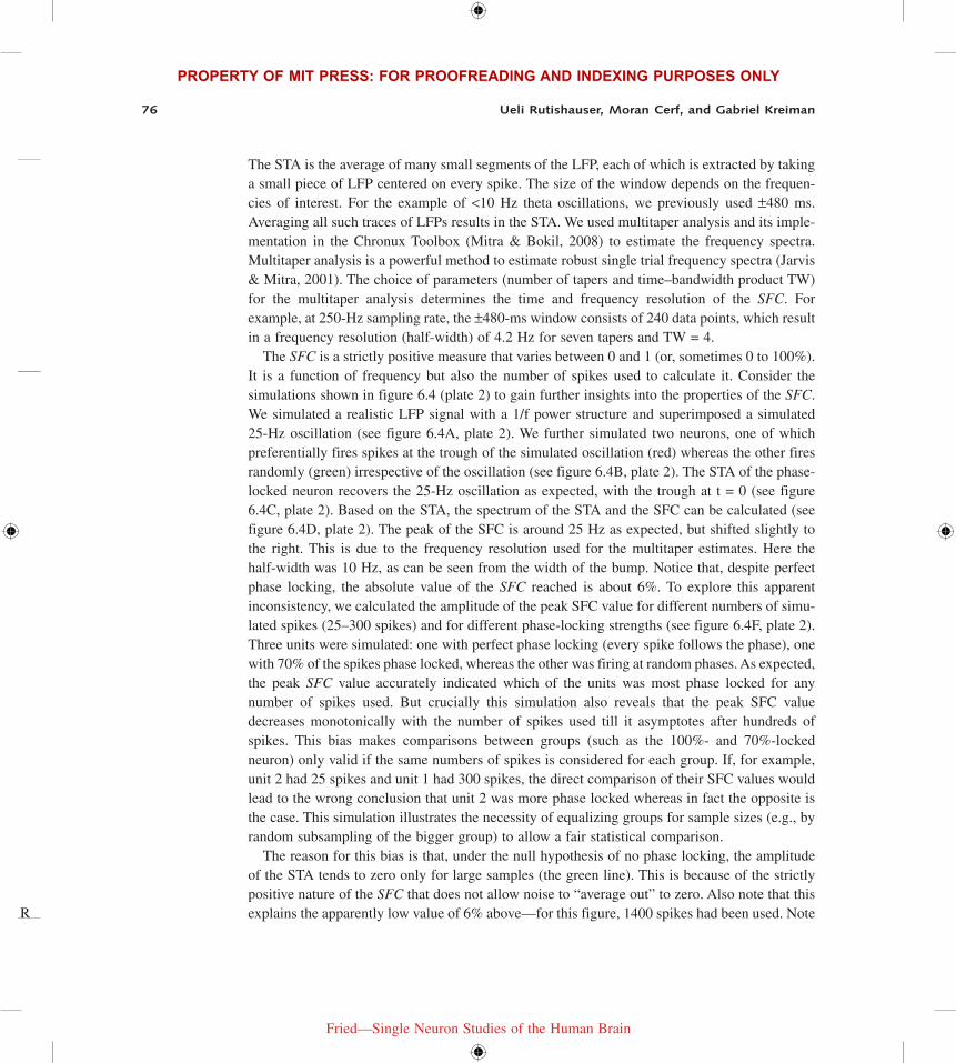
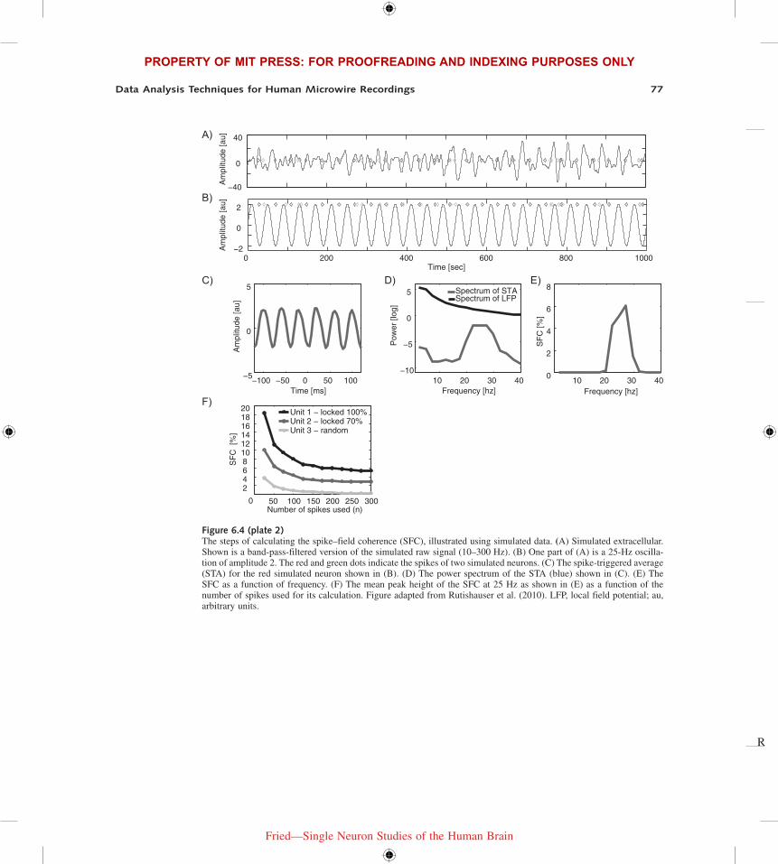
The SFC is a strictly positive measure that varies between 0 and 1 (or, sometimes 0 to 100%). It is a function of frequency but also the number of spikes used to calculate it. Consider the simulations shown in figure 6.4 (plate 2) to gain further insights into the properties of the SFC. We simulated a realistic LFP signal with a 1/f power structure and superimposed a simulated 25-Hz oscillation (see figure 6.4A, plate 2). We further simulated two neurons, one of which preferentially fires spikes at the trough of the simulated oscillation (red) whereas the other fires randomly (green) irrespective of the oscillation (see figure 6.4B, plate 2). The STA of the phase-locked neuron recovers the 25-Hz oscillation as expected, with the trough at t = 0 (see figure 6.4C, plate 2). Based on the STA, the spectrum of the STA and the SFC can be calculated (see figure 6.4D, plate 2). The peak of the SFC is around 25 Hz as expected, but shifted slightly to the right. This is due to the frequency resolution used for the multitaper estimates. Here the half-width was 10 Hz, as can be seen from the width of the bump. Notice that, despite perfect phase locking, the absolute value of the SFC reached is about 6%. To explore this apparent inconsistency, we calculated the amplitude of the peak SFC value for different numbers of simu-lated spikes (25–300 spikes) and for different phase-locking strengths (see figure 6.4F, plate 2). Three units were simulated: one with perfect phase locking (every spike follows the phase), one with 70% of the spikes phase locked, whereas the other was firing at random phases. As expected, the peak SFC value accurately indicated which of the units was most phase locked for any number of spikes used. But crucially this simulation also reveals that the peak SFC value decreases monotonically with the number of spikes used till it asymptotes after hundreds of spikes. This bias makes comparisons between groups (such as the 100%- and 70%-locked neuron) only valid if the same numbers of spikes is considered for each group. If, for example, unit 2 had 25 spikes and unit 1 had 300 spikes, the direct comparison of their SFC values would lead to the wrong conclusion that unit 2 was more phase locked whereas in fact the opposite is the case. This simulation illustrates the necessity of equalizing groups for sample sizes (e.g., by random subsampling of the bigger group) to allow a fair statistical comparison.

The reason for this bias is that, under the null hypothesis of no phase locking, the amplitude of the STA tends to zero only for large samples (the green line). This is because of the strictly positive nature of the SFC that does not allow noise to “average out” to zero. Also note that this explains the apparently low value of 6% above—for this figure, 1400 spikes had been used. Note



R


Am

plitu

de [a

u]

0 200 400 600 800 1000−2

0

2

Time [sec]

Am

plitu

de [a

u]

50 100 150 200 250 3000

2468101214161820

Number of spikes used (n)

SF

C [

%]

Unit 1 − locked 100%Unit 2 − locked 70%Unit 3 − random

−100 −50 0 50 100−5

0

5

Time [ms]

Am

plitu

de [a

u]

10 20 30 40−10

−5

0

5

Frequency [hz]P

ower

[log

]

10 20 30 400

2

4

6

8

SF

C [%

]

Spectrum of STASpectrum of LFP

Frequency [hz]

−40

0

40

Figure 6.4 (plate 2)The steps of calculating the spike–field coherence (SFC), illustrated using simulated data. (A) Simulated extracellular. Shown is a band-pass-filtered version of the simulated raw signal (10–300 Hz). (B) One part of (A) is a 25-Hz oscilla-tion of amplitude 2. The red and green dots indicate the spikes of two simulated neurons. (C) The spike-triggered average (STA) for the red simulated neuron shown in (B). (D) The power spectrum of the STA (blue) shown in (C). (E) The SFC as a function of frequency. (F) The mean peak height of the SFC at 25 Hz as shown in (E) as a function of the number of spikes used for its calculation. Figure adapted from Rutishauser et al. (2010). LFP, local field potential; au, arbitrary units.



R



that this reinforces the point that the SFC is a relative measure—its actual amplitude is not meaningful, but what is meaningful is the proportional difference between two groups (such as the SFC is 50% bigger in group A compared to group B). Recent new methodological develop-ments (Grasse & Moxon, 2010) have also led to the proposal of an analytical method to correct for this bias.

Decoding Brain Signals in Single Trials

Once we have detected spikes, separated them into clusters, and analyzed their relationship with LFPs, we are often interested in correlating the neurophysiological responses with aspects of the cognitive tasks under study (e.g., memory formation, stimulus presentation, attentional modulation, reaction times, etc.). The brain needs to be able to act upon the neurophysiological data in single trials. While averaging over trials is commonplace in an attempt to get rid of noise in many studies, neurons do not have that luxury.1 Also, several practical applications such as driving prosthetic limbs based on the activity of a population of neurons (see chapter 17) require decoding responses in single trials. Here we provide an overview of the math, algorithms, and methodology that underlie decoding the activity of an ensemble of neurons in single trials. For a more detailed discussion of the mathematics of machine learning, we refer the reader to Bishop (1995), Vapnik (1995), and Poggio and Smale (2003). For a more extensive review of feature expression for machine learning and decoding approaches, see Meyers and Kreiman (2011) and Singer and Kreiman (2012).

We focus our discussion on decoding the activity of ensembles of spike trains or LFPs. To provide a concrete example, we imagine a scenario where the subject was presented with n stimuli labeled S Sn1, ,… over multiple trials in pseudorandom order. The exact details of the experimental paradigm are not relevant here. S Sn1, ,… could represent n different pictures, or n different motor commands, or behavioral measures such as correct recollection or not. In any given trial k, we want to examine the neurophysiological recordings and make an educated guess about which experimental condition was presented (k nS Sλ ∈{ }1, ,… denotes the condition for trial k).

Feature ExtractionThe first question that arises in this procedure involves extracting relevant features from the input signals. This constitutes a critical step. If the features extracted from the data do not contain information about the experimental conditions, no machine-learning algorithm will be able to magically lead to decoding performance above chance levels.

We consider a set of spike trains k i k ij

j

s t t t( ) ( )= −=

∑δ1

, where k ijt denotes the timing of spike

j from neuron i (i n= …1, , ) in trial k measured from trial onset. In the interest of simplicity, we consider a simple feature, namely, the spike count, which has historically been shown to convey interesting information: k i k i

w

x w s t dt[ ] = ( )∫ , where w denotes a window of interest. The



R


spike count defined here is by no means the only feature of interest. Other features that have provided interesting information include the number of spikes that are correlated across multiple neurons, the projections onto the first principal components, the coherence between spikes and LFPs, the power of the spike train in specific frequency bands, and so on. While in the definition above k ix w[ ] is a scalar, one could also consider feature vectors such as k i k i ux w x w1[ ] … [ ][ ], , where the feature of interest is computed in multiple temporal windows w1,…,wu within trial k.

It is also of interest to decode LFP signals. It should be noted that the brain does not have direct access to LFP signals. Except for small effects of extracellular fields (Anastassiou et al., 2011), postsynaptic neurons need to make their decisions (to spike or not to spike) based on the incoming set of spike trains from presynaptic neurons. Still, LFPs have often been shown to contain interesting information, their signals can be correlated with spike trains (see “The Rela-tion between Spikes and the LFP”), they may be more readily accessible in situations where spike recordings are not possible and can also have interesting practical properties such as increased stability. In the interest of simplicity, we extract the total power in the LFP signal (L(t)) in a given window w: k i k i

w

x w L t dt[ ] = ( )∫ 2 . Again, there are multiple other possibilities including

considering the power restricted to certain frequency bands, the phase of the signal, the coher-ence between LFPs recorded from different electrodes, and so on. As described above for spike trains, the feature of interest can be extracted in multiple windows w wu1, ,… .

It is worth mentioning several practical considerations. It is often of interest to compare decoding performance of multiunit activity versus single unit activity obtained after spike sorting (see the “Spike Detection” section in this chapter). Nonstationarities abound in neurophysiologi-cal recordings; it is a good idea to attempt to eliminate such nonstationarities before attempting to decode information (Meyers & Kreiman, 2011). In several cases, investigators have considered ensembles of neurons that are not recorded simultaneously (e.g., Hung et al., 2005, as opposed to simultaneous recordings in Wilson & McNaughton, 1993). These ensembles are referred to as pseudo-populations and assume that the responses are independent (i.e., decoding the activity of pseudo-populations does not take into account potential interactions across neurons; Meyers & Kreiman, 2011).

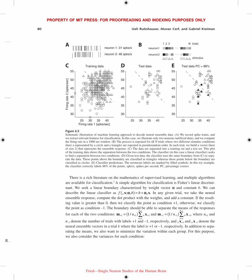
Learning from ExamplesDecoding neural data using machine learning techniques constitutes a typical example of super-vised learning from examples. We have a set of data k k k k nx x xx = …[ ]1 2, , , and a set of labels for each trial k nS Sλ ∈ …{ }1, , . The goal is to build a classifier that can learn the structure of the relationships between k x and k λ. The typical procedure is shown in figure 6.5, where, for illus-trative purposes, we consider n = 2 neurons and only two possible labels (k λ is a circle or a triangle, which we denote as +1 and –1, respectively, in the next paragraph). After extracting relevant features from each neuron (see figure 6.5A–B), we seek a boundary that can separate the two labels. In this case, we show a linear boundary.



R



There is a rich literature on the mathematics of supervised learning, and multiple algorithms are available for classification.2 A simple algorithm for classification is Fisher’s linear discrimi-nant. We seek a linear boundary characterized by weight vector α and constant b. We can describe the linear classifier as f b bk kx x; ,a a( ) = + . In any given trial, we take the neural ensemble response, compute the dot product with the weights, and add a constant. If the result-ing value is greater than 0, then we classify the point as condition +1, otherwise, we classify the point as condition –1. The boundary should be able to separate the means of the responses

for each of the two conditions: m x+ + +=

= ( )+

∑1 1 11

11

/ n kk

n

and m x− − −=

= ( )−

∑1 1 11

11

/ n kk

n

, where n+1 and

n−1 denote the number of trials with labels +1 and –1, respectively, and k x+1 and k x−1 denote the neural ensemble vectors in a trial k where the label is +1 or –1, respectively. In addition to sepa-rating the means, we also want to minimize the variation within each group. For this purpose, we also consider the variances for each condition:

neuron 1: 31 spks/s

neuron 2: 46 spks/s

25 30 35 40

30

35

40

45

50

55

Firing rate 1 [spks/sec]

Firi

ng r

ate

2 [s

pks/

sec]

Training data

25 30 35 40

30

35

40

45

50

55

Test data

25 30 35 40

30

35

40

45

50

55

Test data PC = 88%

A

C D E

trialsneuron1

neuron2

. . .

. . .

1 2 3 NB

stimulus

Figure 6.5Schematic illustration of machine learning approach to decode neural ensemble data. (A) We record spike trains, and we extract relevant features for classification. In this case, we illustrate only two neurons (artificial data), and we compute the firing rate in a 1000-ms window. (B) The process is repeated for all N trials where two different stimulus conditions (here a represented by a circle and a triangle) are repeated in pseudorandom order. In each trial, we build a vector (here of size 2) that represents the ensemble response. (C) The data are separated into a training set and a test set. This plot of the training data shows the separation between the two conditions. The classifier (in this case a linear classifier) seeks to find a separation between two conditions. (D) Given test data, the classifier uses the same boundary from (C) to sepa-rate the data. Those points above the boundary are classified as triangles whereas those points below the boundary are classified as circles. (E) Classifier predictions. The erroneous labels are marked by filled symbols. In this toy example, the classifier correctly labels 88% of the points. spks/s, spikes per second; PC, percentage correct.



R


G+ + + + += −( ) −( )1 1 1 1 1k kT

kx m x m and G− − − − −= −( ) −( )1 1 1 1 1k k

T

kx m x m (6.7)

The Fisher linear discriminant seeks to find the value of the weights α that maximizes the fol-lowing expression:

ˆ. .

aaa G G a

=−( )( )+( )

+ −

+ −arg max

α

T

T

m m1 12

1 1

(6.8)

subject to a = 1. It can be shown that this expression is minimized when

G G a+ − + −+( ) = −1 1 1 1. m m , (6.9)

which can be easily solved using MATLAB. While it is always advisable to write your own code, MATLAB has an implementation of a simple linear discriminant classifier in the clas-sify function. Figure 6.5C–E shows how a line can separate the data and minimize the clas-sification error.

Support vector machines (SVMs) constitute a robust type of classifier that has proven to be successful in many neural decoding applications (as well as in many other domains). For a description of the mathematical principles behind SVM classifiers, see Vapnik (1995) and Cris-tianini and Shawe-Taylor (2000). There are multiple freely available implementations of SVM classifiers including one in MATLAB’s svmtrain and related functions.

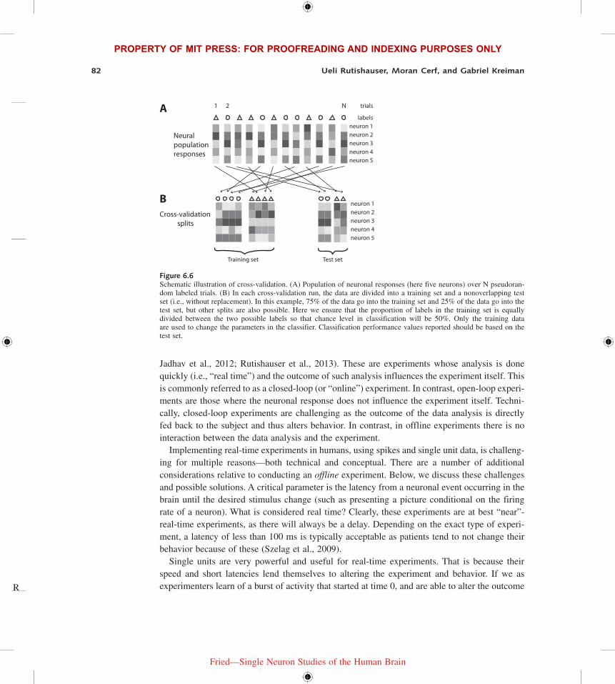
Cross-validationA critical component of all the decoding approaches is to perform cross-validation by separating the data into a training set and a test set. Failure to do so leads to overfitting the data. Depending on the exact characteristics of the problem, dimensionality and number of trials, overfitting can lead to overoptimistic measures of performance and hence misleading conclusions.

A schematic illustration of a typical cross-validation procedure is shown in figure 6.6. Essen-tially, a random subset of the data is used for training (i.e., finding the classifier parameters) and the remaining data are used for evaluating the performance of the classifier. The process is also emphasized in figure 6.5: part C shows the data used to find the parameters of the Fisher linear discriminant, and the resulting boundary line was applied to novel data shown in part D to lead to the classification results shown in part E. For a longer discussion of cross-validation proce-dures, see Meyers and Kreiman (2011).

Real-Time Feedback from Spikes for Closed-Loop Experimentation

Our world is continuous. Therefore, experiments that show discrete presentations of stimuli or are broken down into blocks or trials are limited in how well they simulate real life. Wanting to better simulate real life, scientists occasionally turn to experiments which modify themselves in real time as a function of some brain activity (Fetz, 1969; Griffin et al., 2004; Cerf et al., 2010;



R



Jadhav et al., 2012; Rutishauser et al., 2013). These are experiments whose analysis is done quickly (i.e., “real time”) and the outcome of such analysis influences the experiment itself. This is commonly referred to as a closed-loop (or “online”) experiment. In contrast, open-loop experi-ments are those where the neuronal response does not influence the experiment itself. Techni-cally, closed-loop experiments are challenging as the outcome of the data analysis is directly fed back to the subject and thus alters behavior. In contrast, in offline experiments there is no interaction between the data analysis and the experiment.

Implementing real-time experiments in humans, using spikes and single unit data, is challeng-ing for multiple reasons—both technical and conceptual. There are a number of additional considerations relative to conducting an offline experiment. Below, we discuss these challenges and possible solutions. A critical parameter is the latency from a neuronal event occurring in the brain until the desired stimulus change (such as presenting a picture conditional on the firing rate of a neuron). What is considered real time? Clearly, these experiments are at best “near”-real-time experiments, as there will always be a delay. Depending on the exact type of experi-ment, a latency of less than 100 ms is typically acceptable as patients tend to not change their behavior because of these (Szelag et al., 2009).

Single units are very powerful and useful for real-time experiments. That is because their speed and short latencies lend themselves to altering the experiment and behavior. If we as experimenters learn of a burst of activity that started at time 0, and are able to alter the outcome

A

Neural population responses

Cross-validation splits

Training set Test set

neuron 1neuron 2neuron 3neuron 4neuron 5

trials1 2 N

labels

neuron 1neuron 2neuron 3neuron 4neuron 5

B

Figure 6.6Schematic illustration of cross-validation. (A) Population of neuronal responses (here five neurons) over N pseudoran-dom labeled trials. (B) In each cross-validation run, the data are divided into a training set and a nonoverlapping test set (i.e., without replacement). In this example, 75% of the data go into the training set and 25% of the data go into the test set, but other splits are also possible. Here we ensure that the proportion of labels in the training set is equally divided between the two possible labels so that chance level in classification will be 50%. Only the training data are used to change the parameters in the classifier. Classification performance values reported should be based on the test set.



R


of a trial in less than 100 ms following this activity, the subject is likely to interpret the entire sequence as happening in real time. More so, given the high SNR of single-unit firing, typically only a few trials are needed to decode the meaning of a certain unit’s firing. That is, we can offer single trial classifiers that operate based simply on separating the baseline activity of the unit and the active firing.

Challenges in Designing Real-Time Experiments

Programming Challenges Much of our programming tools were designed for offline experi-ments where time is effectively set by internal mechanisms that are placed in the code. That is, a typical stimulus presentation routine would present an image on the screen and then wait for 1 s before removing the image from the screen. In contrast, in online experiments we often have to hold a variable that measures the time from previous events. That is, a code block that performs the same function in a real-time experiment will often start with a line that sets the time variable to the current time, and then starts a while loop that asks whether one second had already passed in which the experimenter would repeatedly pull information from the brain, for example, and exit the loop to remove the image from the screen. This is mostly true for closed-loop real-time experiments where data are being analyzed continuously and processing time is sometimes a bottleneck that experimenters want to overcome by not operating sequentially but rather using the delay time (in this example 1 s) to perform some of the analyses.

Another challenge with online experimental implementation is the tight integration with the acquisition system or simulations thereof for testing and debugging. Therefore, the experimental code will have to include acquisition-system-specific calls to interact with the acquisition system to receive data. This implies that the experiment itself has to be implemented in a way that permits inserting such commands. This typically prohibits using closed-source systems such as those frequently used in visual psychophysics and a number of popular tools in experimental design, which do not support such interaction. Testing and debugging such an approach is chal-lenging. Ideally, the same experimental code can be used for both an actual patient and a “simu-lated” situation where simulated data are used or previously recorded data are replayed. Finally, an additional challenge in real-time coding involves controlling the flow of experiment time in the event of unexpected circumstances.

Real-time approaches are frequently used in other fields (i.e., electrical engineering, gaming), allowing us to adapt existing and proven methods. Below, we outline two solutions that we found useful in implementing our closed-loop experiments (Cerf et al., 2010).

Event-Based Programming An efficient way to handle real-time coding is “event based pro-gramming,” which uses the operating system’s event queue. This allows processes and methods to “register” with an event manager, which in turn calls the registered function when a certain event has occurred (“callback”). For example, instead of having a while loop that checks at the end of each cycle whether a button was pressed, you register a function to be called when a



R



button has been pressed with the event manager, and whenever the button is pressed, this func-tion is called automatically. One can set functions that are based on events occurring, on the period occurrence of a particular event (say, call a function that pulls data from the brain repeat-edly every millisecond or every 100 ms regardless of the linearity of the code), or events that happen a period of time following a certain event (say, run a function exactly 300 ms after a button was pressed).

Most programming languages and operating systems offer event-based processing. In the following, we use MATLAB to illustrate examples, but similar commands can be used in other environments. The main functions in MATLAB for event-based coding are: “timer” and “addlistener.”

The addlistener object registers a listener with the event handler, which starts the event process. The listener uses strings to capture events (i.e., using ‘ButtonPressed’ as a trigger that indicates the event that marks a button press).

The “timer” function allows for setting delays or precise or periodic timing. For example, setting the ‘StartDelay’ attribute instructs the timer to trigger an event after a certain delay. Calling start(eventlistener) and stop(eventlistener) controls the flow of the experiment. That is, at the end of each trial, for example, we can ‘stop’ all listeners and then re-‘start’ them at the beginning of a future trial.

Finally, it is important to note the numerous variants of the timer function that really allow for optimized control of the experimental timing, with the ability to set time for a certain time, for a periodic recurring call (using the ‘Period’ attribute), for a specific delay, or for a delay from the occurrence of a certain future event.

Clock-Slowing Debug Debugging real-time code is challenging. Frequently, specific events can only occur in short windows of opportunity, such as when a particular neuronal event occurs within 100 ms after the subject presses a button. When testing code—for example, by line-by-line execution—such time conditions cannot be satisfied. How can this code be debugged then? MATLAB and various other OS implementations now allow you to ‘slow time.’ Meaning—one can decide that every processor cycle (the metric used to count time in computers) will account for a different time unit. As in—instead of one CPU cycle accounting for 1/3500 MHz, one can decide that it will actually account for 1 s, therefore providing a slow run of everything. This allows for effective real-time debugging. Obviously the brain still works at the same speed in the real-time environment, so one needs to think of “slowing down the input to the code as well,” but given that oftentimes when debugging real-time codes we are working with simulators (see the next paragraph), we should be able to either get “slower brains” by slowing the OS altogether, making our spikes simulator slow as well, or by tweaking our spike generator to simply work at a much lower sampling rate.

Simulating a Brain Time working with the patient is the most precious of commodities in single neuron recordings, requiring careful testing before performing experiments. Below, we outline



R


methods we found useful: (1) using prerecorded brain data, (2) using existing brain simulators, and (3) generating random spikes. The second and the third options utilize simulated data, with the difference being that one is using a simulator that was provided by a vendor or by the acqui-sition system (those are now widely supported by many vendors) while the other is generating simulated spikes. Simulators nowadays can go from simple (generating spikes at a Poisson distribution with a given rate for each of multiple neurons—where the parameters can often be tweaked to some extent) to much more complex simulators that actually were designed to simulate a particular brain area or neuronal behavior (i.e., a neuron which changes its firing rate based on event triggers from the environment—equivalent to its preferred stimulus being presented).3

Performance Issues When discussing real-time processing, one question that arises is the notion of timing in the brain. A vast literature has explored the notion of time perception, the effects of minor delays on the perception of real time, and the psychology of “now.” We won’t address any of these questions in this chapter other than to state that studies (Szelag & Poppel, 2000) suggest that with small variability humans perceive events that happen with a delay of over 100 ms as certainly lagging. That is, if your keyboard would respond to your key presses with the tiny delay of 100 ms, this would surely be noticeable by you and presumably lead you to use a different keyboard. Therefore, when we come to design real-time experiments, and depending on the questions and task, we have to set some boundaries to what constitutes real time and what delays we accept in our code. Given that the short delay between the moment in which a neuron in the brain spiked to the moment it somehow changed the experiment and was perceived by the patient is in milliseconds, we need to make sure that all our analyses and according experi-mental modification happen within that small timescale. There are a number of performance considerations that should be taken into account in order to minimize the latency between neu-ronal responses and the desired effects.

First, frequently the analysis of data from an individual recording channel is identical to that from other channels. Thus, parallel processing can be used to take advantage of the recent increase in the availability of multiple CPUs/GPUs/cores. Second, there are many speed improve-ments that can be utilized by appropriate programming techniques. For example, in MATLAB, preallocating arrays rather than having those grow in size during runtime can affect speed greatly. Usage of correct logical operators (| for array elements versus || for scalar values) improves performance. When using compiled languages such as C or Java, the compiler itself has a set of flags that can be used to improve real-time performance at the expense of memory.

Generally, real-time programs tend to be harder to read because they occasionally improve efficiency at the expense of proper coding. However, some simple tricks can aid in improving and analyzing the codes’ performance bottlenecks. CPU timing metrics like the ‘tic’/’toc’ com-mands in MATLAB indicate locations where runtime operations spend more time than others. In addition, many languages including MATLAB and C have a variety of “profiling” tools that enable the debugging of code timing following a run.



R



Here are a few typical bottlenecks in real-time experiments:

Networking Conducting closed-loop experiments frequently requires using multiple hardware systems (such as for acquisition, data analysis, and stimulus display) that need to exchange large quantities of data among them. This requires a fast and dedicated network among those machines. Additional parameters that affect network congestion and speed include the type and amount of data used. Acquisition systems deliver data of several types: raw continuous data, filtered con-tinuous data, spike waveforms after a threshold was applied by the acquisition system, clustered spikes/shapes after they were thresholded and sorted, only the spike peak times, or just the number of spikes within a window (firing rate). Additionally, the amount of data is also influ-enced by the size of the window of time used to retrieve data, the sampling rate, and the number of channels. Some systems allow the user to control these parameters remotely while others do not. For instance, at present the Blackrock system allows only a choice between continuous, or spikes and shapes; and data are only delivered for all recorded channels together at the sampling rate at which the data were recorded (i.e., there is no possibility to subselect a range of chan-nels). We advise using a local area network with its own routers and switches and short cabling to allow for rapid data transfer.

Computer performance Performance of the hardware/software system itself can greatly affect the speed and precision of online analyses. Open processes, small paging files, or unexpected update checks can harm our experiments. There are tools to remove all but the essential processes when crucial experiments are run, and multiple companies specialize in real-time performance tweaking. First, if possible, minimize the displays. Many acquisition applications show spikes and continuous data on the screen, which can slow down processing. Also, channels which do not yield useful data should be removed from the recording and analysis entirely to save band-width and computing power. Also, depending on the analysis performed, the sampling rate can be reduced. Finally, visualization can be minimized to reduce the load. One additional recom-mendation is to keep the configuration file used for each and every experiment together with the experiment files.

Online Data Access through Application Programming Interfaces (APIs)The authors of this chapter have worked with two acquisition systems thus far: Neuralynx Cheetah, and Blackrock’s Neuroport. The following briefly outlines their methods and what consideration one needs to take into account when handling those.

Blackrock’s Neuroport—CBMex Without going into specific details of the system (which are likely to change rapidly) we will briefly discuss the main logic of the CBMex environment and the main considerations to account for when using it.

CBMex was not written by Blackrock. This means that parts of the code were tailored to very specific needs rather than general users. Currently CBMex is supported only on PC computers



R


with the requirement of a matching CBMex to each Firmware version of Neuroport (i.e., if the Neuroport firmware is upgraded, CBMex must be upgraded also).

CBMex provides the standard commands required from an online application—connecting to the Neuroport locally or remotely (“cbmex(‘open’)”), syncing the clocks of the acquisition system and the experimental machine (“cbmex(‘time’)”), which is the effective synchronization of the remote and acquisition systems, the start of a recording buffer (“cbmex(‘trialconfig’)”), and the polling of data (“cbmex(‘trialdata’)”). Data is polled from the last time the buffer was emptied in every poll, and the parameters of the command determine whether one wants the continuous data in full or simply the spikes structure. The window of time used is a buffer that can get full if data isn’t pulled often enough. When the buffer is full, data is overwritten in a circular fashion. The documentation says that pulling every 3 s is safe, but tests we have done show that based on standard computers out there, one can in fact pull data from even much longer windows (~10 s) and still not lose any data. The connection and data transfer is done via the User Datagram Protocol (UDP), and the protocol as well as the actual CBMex C code are readily available.

Notably, the interaction between the Neuroport system and the PC (currently the only OS) computer which manages the acquisition (start, stop, file names, etc.) can be done using cbmex as well (“cbmex(‘fileconfig’)”). CBMex allows for sending triggers from the code to the system, alerting on certain events as well, and altogether gives the basic required functionality.

One major conceptual problem in the current version of the system has to do with certain race conditions that can exist between the cbmex initialization and the acknowledgment from the Neuroport that often results in a crash or freezing of the interaction and an ultimate crash of the MEX interpreter and, subsequently, of MATLAB. This is caused if two cbmex commands are sent in sequence but arrive in conflicting order—say, cbmex(‘open’) followed by cbmex(‘trailconfig’)—which often results in a crash. The simple workaround involves imposing a short pause between the commands, which is long enough to ensure the arrival of one before the other (this is a UDP-related problem that is often occurring in protocols of that nature). The above code would then be translated to the following: cbmex(‘open’); pause(0.1); cbmex(‘trialconfig’); this is enough to solve this problem.

Neuralynx’s Cheetah—NetCom Neuralynx offers a .NET-based API “NetCom” to interact with the acquisition system. It can therefore interact with any language that supports .NET, including MATLAB. NetCom acts as a client to the Cheetah acquisition server. However, contrary to the Neuroport, which broadcasts its data over the network to the ‘network address’ (x.x.x.128), NetCom uses a single communication channel and requires registering to open the data. This is effectively similar still to Neuroport since the cbmex(‘open’) command effectively operates as a single channel of transport. Only a single Netcom client can directly communicate with the acquisition system. However, Neuralynx provides an additional program called the “Netcom router” that permits multiple clients to connect to the acquisition system.



R



NetCom provides commands such as “NlxConnectToServer” to connect to the acquisition system or router or “NlxGetNewCSCData” to receive new data.

Netcom’s strategy is to separate the connection to the server from the data streams themselves, which allows for exchange of system commands before choosing which data to use. Netcom follows a subscription model: Each client can specify which data channel(s) to subscribe to and then subsequently poll data from only this subset of channels. In comparison to Neuroport, NetCom provides more choices to users such as choice of channels and objects to load and does not require the polling of all the objects for any given query. For example, users can first request a list of available objects using “NlxGetCheetahObjectsAndTypes()” (where objects include continuous and spike channels, Event (TTL) channels, video channels, etc.). This is then fol-lowed by a choice of which data to subscribe to by indicating to NetCom the relevant streams. Data is streamed in blocks of 512 samples, which can create some difficulties requiring the client to wait for the next buffer in order to get a full spike shape if it happened to be at the edge of a 512-sample block. Table 6.1 compares the features of online data access provided by the Neuroport and Cheetah.

Data Analyses Challenges

Real-Time Experiment Decisions Unlike offline experiments, which can be analyzed in multiple ways after finishing the experiment, online experiments suffer (and benefit) from the fact that the analysis has to be structured before running the experiment. That is because the experiment flow is part of the analysis and is affected by it. If an experiment tests some learning effect, for instance, and makes the trials harder or easier based on the performance on previous trials, then

Table 6.1Comparison of the features of online data access provided by the two Food and Drug Administration–approved systems at time of writing

Feature Blackrock Neuroport Neuralynx Cheetah

Ability to select a subset of objects rather than all existing objects

– +

Multiple clients can connect + + (With NetCom router)Company-provided and supported code – +Support – +Ability to read separately video data, events, spikes data, etc. (Blackrock only events, spikes)

– +

Documentation Partial; not used much and not debugged much

Partial, not used much but exists; the documentation file format is Windows only

Support for other platforms – (Only PC at present) All .NET platforms (effectively only PC)Minimal latency possible 1 ms 15 ms (due to 512 samples transfer block

size for continuous data)Ability to receive data at lower sampling rate or with different filters than recorded

– +



R


nearly every experimental run is going to be different for each patient and each session, based on the performance in that very run. That is, the experiment will rarely be exactly the same when repeated twice. Thus the analysis has to take this difference into account and still be able to draw overall conclusions about the population. For example, if learning affects the performance of the patient in the next trial, then the experimental information that led to it must be used for the analysis.

Choices of parameters and analysis methods cannot be changed post hoc, as is usually done. Here is an example of this: In an experiment run by one of the authors (MC) the decision was made that the analysis of spikes would be done on multiunits rather than on online sorted data since the sorting time would slow the processing too much, which could affect the actual runtime decisions (the patient would become aware of the fact that there is a delay between his or her thoughts and their manifestation on the experimental computer; see Cerf et al., 2010). The deci-sion was therefore made to use only unsorted spikes for the experiment. The analysis of existing data showed that this would introduce a certain level of noise, but we felt that the patients would be able to perform well nevertheless. Once the data were collected, we proceeded to perform detailed offline analysis including careful spike sorting to look at the single units that drove the results. While the results were a little different (2% improvement in the performance would have been achieved from single units) we cannot with confidence know the extent of the actual improvement that would have been observed in reality. We cannot say that using single units would have been simply an improvement on using the multiunits, because the additional hidden variable here is how it would affect the patient’s performance. It is conceivable that running the experiment with single units would make the patient “work harder” or try different strategies to control the particular brain–machine interface that was used in the experiment, and therefore the performance would have been much improved (or vice versa: maybe the patient would have lost interest and tried less hard since things would be great early on). Simply put, there is no way to draw a conclusion on what would have happened were the experiment conditional on different data than the ones used in the actual experiment.

Choice of Data to be Analyzed Similar to the previous point, we feel the need to emphasize that, more so than in other experiments, online experiments can benefit significantly from prior knowledge on the properties of the neurons one records from.

That is, if one has the capacity (time, patient time, human hours, etc.) to arrive at the patient’s room prior to the experiment, acquire data before the beginning of the experiment, and tailor the variables to the particular experiments, this always proves invaluable. In our ideal experi-ments we set the thresholds and sorting algorithms for the particular patient’s needs before experiments start. Then the experiment is run, and the parameters are saved and fixed and used throughout.

Here’s a concrete example of such: The Cheetah system, as was mentioned earlier, is able to separate the channels read during the experiments and transfer to the analysis computer only a small set of relevant channels. In the study by Cerf et al. (2010) it became clear to us that we



R



would need to look at the raw data from the acquisition system and filter/threshold/analyze it locally ourselves rather than relying on the filtering done by the acquisition system. Transferring the raw data of a few seconds of multiple channels can be taxing on the network and could lead to an overwhelming strain on the acquisition system that could end up delaying processing or affecting the experiment. Therefore, we began every experiment by a prescreening of the units to be used in the experiment, and we decreased the dimensionality of our units to only channels that had uniquely responsive units (i.e., units responding to stimuli which were not repeated in other channels). This typically decreased the number of channels we looked at from 64 to about 5. This allowed us to focus on smaller amounts of data, and we could even focus on tweaking some of our decoding parameters to the nature of those channels (mainly, how we normalized the firing rates). This only came from knowing our data well and, particularly, knowing that some units in areas like the parahippocampal cortex have higher firing rates and will result in more demanding bandwidth needs than others; this even allowed us to separate in the code the retrieval of channels at different times within our 20-ms window to make sure we controlled the flow of information and analyses. These are the types of knowledge that are hard to change later as suggested in the previous section but could improve the analyses significantly.

Experimental choices for real-time data processing include using multiunits or single units; using raw data or only spikes, LFPs, or firing rates; using all channels or a smaller number of channels; acquiring and sampling all channels or only some (usually one would want all here at the highest sampling rate unless this really poses a strain on the acquisition system); and deciding what network architecture to use.

Bandwidth and Processing Time In the context of real-time experiments the following variables can impact performance:

Bandwidth = <number of channels> x <window of activity> x <sampling rate>Data arrival latency = <bandwidth> / <network congestion >Processing time = <data arrival latency> + <filtering time> + <spike detection time> + [spike-sorting time]

The main choices we can control are the number of channels used for the analysis and the window of activity used. The bandwidth is also governed by the type and formatting of the data. We often consider three data types: the entire continuous data (LFPs), filtered or unfiltered; the thresholded data (spikes); or the firing rate. Bandwidth requirements differ significantly among these.

Storage of Experimental Data Unlike offline experiments, where the analyses can be fully reproduced postexperiment, the variables in real-time experiments are part of the experiment. As such, it is essential in real-time experiments to maintain as many of the environmental con-ditions and variables as possible. In order to do so, saving all the data every few trials is recommended.



R


On the acquisition system side, storing data in the most raw form possible is advantageous. Some systems offer two ways of storing data to facilitate this—in a compact format for future analysis, in addition to a raw format. For example, the Cheetah system saves the filtered continu-ous data in individual files, one for each recording channel. However, an additional file (“NDMA file”) can also be stored, which contains all recorded data in its raw form before filtering (similar to the structure used by Neuroport). This file is very large (for example, 40 GB/h for a 64-channel system) but can be used to fully replicate the experiment offline (“replay”). Such data replay is an excellent means for system development.

Experimental ChallengesFinally, we will address some of the challenges that need to be noted simply due to the running of an experiment online.

Architecture Figure 6.7 (plate 3) illustrates a typical online experimental setup. Wires lead from the patient’s brain directly to the acquisition system, from which the data are transferred over the network to an additional computer (either directly to the experimental computer or, prefer-ably, to a dedicated computer for data analysis), and then, after a decision is made based on the previous data, ultimately fed into the experimental computer to drive the machine in the brain–machine interactive setup.

5

Acquisition

Spike detection and sorting

Decoding

Figure 6.7 (plate 3)Illustration of a typical online experimental setup.



R



Real-time experiments present a technical challenge beyond simply setting up a laptop in front of the patient. Instead, a cluster of computers is typically required. In the authors’ experience, these challenges end up being difficult to handle. Problems include setting up a network locally, making sure that all computers communicate with each other, and trying to replicate the condi-tions as much as possible each time (use the same bandwidth, use the same cables, use the same network architecture, etc.).

One versus Multiple Trials An ideal online experiment is one in which decisions effectively are made in runtime using the data from only one trial. That is, some occurrence in the envi-ronment is analyzed in real time and affects the experimental flow immediately. This is hard to do. Decoders often need a significant number of preluding training trials before they can arrive at the stage where a choice can be made over one trial in real time, and many codes will never reach this threshold due to a number of possible problems (decoder, data recorded, noise, etc.). This means that the experimenter will have to make choices in the experiment as to what level of decoding performance is required, how many trials are used for training, and then how many trials are used to make a decision. Each experiment has different needs, and the data drive much of these decisions, but one of the main advantages of single neuron record-ing is that we can aim for single trial decoding of choice and behavior, unlike with other methods.

In his classical “volition” experiment, for instance, Benjamin Libet could see the principal result (the readiness potential) only by averaging dozens of electroencephalography (EEG) trials. This is still true to date even with the improvement of EEG acquisition methods. Analysis based on LFPs (or ECoG) of single trials is possible (Chen et al., 2013; Maoz et al., 2012) but suffers from the same limitations to some degree. However, recent online experimentation in real-time single neuron recordings in humans (Cerf et al., 2010) and analysis of offline experiments as if they were online—to test the potential ability to have analyzed data in single trials (Quiroga et al., 2007; Fried et al., 2011)—suggest that the data have the potential of being ideal for these types of experiments.

Training Length While the decoding literature suggests ways to estimate the optimal level of training a decoder requires in order to reach best results in the eventual testing phase, online experiments often cannot abide by these calculations. This is merely because we are also bound from above by the patient and clinical constraints. One way to decide when to end the training phase and advance to the testing phase is simply to set a fixed predetermined performance threshold and lock the parameters (or keep updating them to improve performance) once the threshold is met. This, however, could result in some runs of the experiment that never arrive at the testing phase. An alternative is, of course, to ignore the performance altogether and just set a fixed number of trials after which the decoder is locked no matter what and is used for testing regardless. The authors have used both methods in the past and currently propose a combination



R


of the two which is not ideal in most experimental conditions but is the optimal one for real-time experiments in humans: fixing a threshold for ideal move to testing, in addition to setting a maximal number of trials at which one shifts to testing regardless of the performance.

Offline Analysis of Online Data One additional recommendation for conducting real-time experiments is to ultimately analyze the data from the online experiment offline later as if the experiment was not run in a closed loop. Such analysis done by Cerf et al. (2010) showed, in fact, that the performance could have improved only slightly from using single units (rather than multiunits), different filtering, and wider windows of brain data polling. While one cannot change any of the analysis parameters post hoc in an online experiment, one can surely use this information for improved future analyses and for future reporting to determine the ideal param-eter for potential online experiments replicating the results or building upon this knowledge. The authors encourage any experimenter considering future online experiments to ultimately report both the results of the online experiment and the results of offline data analyses.

Philosophical and Ethical Considerations in Real-Time Closed-Loop ExperimentsChapter 4 discussed important ethical considerations with respect to recording data from human patients. Here we extend some of those considerations in the particular context of real-time closed-loop experiments.

While our behavior is controlled by our brain at all times, we have the subjective experience (perhaps illusory) of an “interaction” between our brain and our reflective consciousness that is very familiar to us. We operate in the world and feel we are the agents of our behavior. Online experiments profoundly change this access architecture by giving patients direct feedback on their brain activity. There are currently probably only a few dozen humans that were actually able to directly hear the activity of their own brain and manipulate their behavior accordingly. We do not know if and how this feeling and unique experience changes behavior. It may very well be that just the sheer access the individual has to his or her brain allows for changes in neuronal patterns. Simply put, it could be that a person who moves a cursor on a screen based on the activity of a neuron is not just reading the neuron’s activity but actually modifying the activity in real time. We currently have no way to separate the two cases or test this difference, but as experimenters we should be aware of this concern and think of ways to figure out what is entailed when giving a person external access to his or her thoughts.

In our online experiments, we pride ourselves on the fact that the patients’ behavior can be manipulated by the experiment itself and feel that we gain unique knowledge about the way in which the brain operates. However, one needs to remember that while this constitutes acquiring a unique and unprecedented access to the brain, this is also a very atypical situation, which is not necessarily representative of normal behavior. One should also note that, in our experience, all (100%) of our patients who participated in online experiments provided feedback indicating that the experience was fascinating and remarkable for them.



R



When and Why to Consider Online ExperimentsA few things make online experiments advisable for scientists venturing into the world of single neuron recordings in humans:

1. Unlike many noninvasive methods, single neuron recordings can make use of real-time infor-mation. Functional magnetic resonance imaging, for instance, does not have sufficient temporal resolution for real-time experiments (with delays of seconds after neuronal activity manifested in the blood-oxygen-level-dependent signal); EEG experiments often require averaging over numerous repetitions in order to arrive at a result that is easily registered in a single trial in the direct readout of a neuron.2. Online experiments are still new and are in many ways an uncharted territory for scientists. This is especially true for human electrophysiology ones. Thus there is ample room to develop and refine new methods.3. Online experiments are typically more engaging for the patients. Given the unique nature of access that the patients have to their own brain, our experience suggests that they are often more likely to find these engaging and try harder and with more enthusiasm to explore the level of access they get to their brain. Real-time experiments tend to be more satisfying for the patients.4. Online experiments allow us to address questions that are at the heart of the most exciting inquiries in neuroscience, such as the nature of free will.5. Finally, real-time experiments give us access to internal processes in a way that is not simply the equivalent of an offline experiment, just done online, but is actually a practice that provides us with the ability to interact with neurons in a way that circumvents some of the internal network flow. By taking the output of one neuron and effectively using it as the input to a new system, we actually, in a simplified way, create connections in the brain that otherwise do not exist. For example, by taking the output of memory cells in the hippocampus and giving the patient direct access to these neurons (as done in Cerf et al., 2010), the network doesn’t just get an additional source of information to interact with but effectively simulates a set of connections from the memory to the visual system, such that input from one feeds into the other. This is something that is not in the original connectivity map but is rather a set of connections that we the experi-menters created effectively. Controlling and wisely choosing which two systems to connect can actually allow us to study interactions that otherwise cannot be tested.

Software

On the website (www.humansingleunit.org) we provide open source software as well as links for many of the algorithms and methodology presented in this chapter. In particular, we include:

• A comprehensive open-source closed-loop framework called StimOMatic (Rutishauser et al., 2013). It offers a flexible software framework that provides a plug-in architecture to facili-tate development of closed-loop experiments. All components discussed in this section are



R


implemented (stimulus display, real-time analysis, continuous and spike-data analysis), and data is processed in parallel on many CPUs/cores in parallel. New functionality can be added by implementing new plug-ins specific to the experiment. These plug-ins are small and self- contained, enabling experimenters to focus on the task at hand. In addition, we provide careful evaluation of the latencies and bottlenecks of the different system components.• Documented object-oriented event-based code used for the experiments in Cerf et al. (2010).• A list of links to several freely available algorithms for machine learning and decoding analyses.• A simulator which allows for setting up of multiple neurons (up to 512 channels at near real time (see note 3).

Notes

1. In some cases, investigators assume that averaging over trials is equivalent to averaging over multiple independent neurons (Parker, A. J., and Newsome, W. T. (1998), “Sense and the single neuron: Probing the physiology of perception,” Annual Review of Neuroscience, 21, 227–277). The extent to which this approximation holds depends on multiple assumptions and remains a topic of debate in the field.

2. The boundary in figure 6.5 was computed using MATLAB’s classify function. A list of links to several freely avail-able algorithms can be found in http://tinyurl.com/klabdecoding.

3. We provide one such simulator on the website www.humansingleunit.org which allows for setting up of multiple neurons (up to 512 channels at near real time), each with its own baseline firing rate, preferred stimulus firing rate, duration, and latency) and the ability to generate single/multiunits per channel. The control of the virtual appearance of the preferred stimulus is governed by external events that can be sent, via TCP/IP, serial port, or direct command, to the listening process, which will alter the particular preferring neurons’ firing rate.

References

Anastassiou, C. A., Perin, R., Markram, H., & Koch, C. (2011). Ephaptic coupling of cortical neurons. Nature Neurosci-ence, 14, 217–223.

Bankman, I. N., Johnson, K. O., & Schneider, W. (1993). Optimal detection, classification, and superposition resolution in neural waveform recordings. IEEE Transactions on Bio-Medical Engineering, 40, 836–841.

Berens, P. (2009). CircStat: A MATLAB Toolbox for Circular Statistics. Journal of Statistical Software, 31, 1–21.

Bishop, C. M. (1995). Neural networks for pattern recognition. Oxford: Clarendon Press.

Buzsáki, G. (2004). Large-scale recording of neuronal ensembles. Nature Neuroscience, 7, 446–451.

Buzsáki, G. (2006). Rhythms of the brain. Oxford: Oxford University Press.

Buzsáki, G., Anastassiou, C. A., & Koch, C. (2012). The origin of extracellular fields and currents—EEG, ECoG, LFP and spikes. Nature Reviews. Neuroscience, 13, 407–420.

Canolty, R. T., Edwards, E., Dalal, S. S., Soltani, M., Nagarajan, S. S., Kirsch, H. E., et al. (2006). High gamma power is phase-locked to theta oscillations in human neocortex. Science, 313, 1626–1628.

Caplan, J. B., Madsen, J. R., Raghavachari, S., & Kahana, M. J. (2001). Distinct patterns of brain oscillations underlie two basic parameters of human maze learning. Journal of Neurophysiology, 86, 368–380.

Cerf, M., Thiruvengadam, N., Mormann, F., Kraskov, A., Quiroga, R. Q., Koch, C., et al. (2010). On-line, voluntary control of human temporal lobe neurons. Nature, 467, 1104–1108.

Chen, L., Madhavan, R., Rapoport, B., & Anderson, W. (2013). Real-time brain oscillation detection and phase-locked stimulation using autoregressive spectral estimation and time-series forward prediction. IEEE Transactions on Bio-Medical Engineering, 60, 753–762.

Choi, J. H., Jung, H. K., & Kim, T. (2006). A new action potential detector using the MTEO and its effects on spike sorting systems at low signal-to-noise ratios. IEEE Transactions on Bio-Medical Engineering, 53, 738–746.



R



Cristianini, N., & Shawe-Taylor, J. (2000). An introduction to support vector machines and other kernel-based learning methods. Cambridge: Cambridge University Press.

Csicsvari, J., Hirase, H., Czurko, A., & Buzsáki, G. (1998). Reliability and state dependence of pyramidal cell–inter-neuron synapses in the hippocampus: An ensemble approach in the behaving rat. Neuron, 21, 179–189.

Donoho, D. L., & Johnstone, I. M. (1994). Ideal spatial adaptation by wavelet shrinkage. Biometrika, 81, 425–455.

Fetz, E. E. (1969). Operant conditioning of cortical unit activity. Science, 163, 955–958.

Fisher, N. I. (1993). Statistical analysis of circular data. Cambridge: Cambridge University Press.

Fried, I., Mukamel, R., & Kreiman, G. (2011). Internally generated preactivation of single neurons in human medial frontal cortex predicts volition. Neuron, 69, 548–562.

Fries, P., Reynolds, J. H., Rorie, A. E., & Desimone, R. (2001). Modulation of oscillatory neuronal synchronization by selective visual attention. Science, 291, 1560–1563.

Fries, P., Roelfsema, P. R., Engel, A. K., Konig, P., & Singer, W. (1997). Synchronization of oscillatory responses in visual cortex correlates with perception in interocular rivalry. Proceedings of the National Academy of Sciences of the United States of America, 94, 12699–12704.

Gabbiani, F., & Koch, C. (1999). Principles of spike train analysis. In C. Koch & I. Segev (Eds.), Methods in neuronal modeling: From synapses to networks (pp. 313–360). Cambridge, MA: MIT Press.

Gibson, S., Judy, J. W., & Markovi, D. (2012). Spike sorting: The first step in decoding the brain. IEEE Signal Process-ing Magazine, 29, 124–143.

Gold, C., Henze, D. A., Koch, C., & Buzsáki, G. (2006). On the origin of the extracellular action potential waveform: A modeling study. Journal of Neurophysiology, 95, 3113–3128.

Grasse, D. W., & Moxon, K. A. (2010). Correcting the bias of spike field coherence estimators due to a finite number of spikes. Journal of Neurophysiology, 104, 548–558.

Griffin, A. L., Asaka, Y., Darling, R. D., & Berry, S. D. (2004). Theta-contingent trial presentation accelerates learning rate and enhances hippocampal plasticity during trace eyeblink conditioning. Behavioral Neuroscience, 118, 403–411.

Harris, K. D., Henze, D. A., Csicsvari, J., Hirase, H., & Buzsáki, G. (2000). Accuracy of tetrode spike separation as determined by simultaneous intracellular and extracellular measurements. Journal of Neurophysiology, 84, 401–414.

Henze, D. A., Borhegyi, Z., Csicsvari, J., Mamiya, A., Harris, K. D., & Buzsáki, G. (2000). Intracellular features pre-dicted by extracellular recordings in the hippocampus in vivo. Journal of Neurophysiology, 84, 390–400.

Hill, D. N., Mehta, S. B., & Kleinfeld, D. (2011). Quality metrics to accompany spike sorting of extracellular signals. Journal of Neuroscience, 31, 8699–8705.

Hung, C. P., Kreiman, G., Poggio, T., & DiCarlo, J. J. (2005). Fast readout of object identity from macaque inferior temporal cortex. Science, 310, 863–866.

Jacobs, J., Kahana, M. J., Ekstrom, A. D., & Fried, I. (2007). Brain oscillations control timing of single-neuron activity in humans. Journal of Neuroscience, 27, 3839–3844.

Jadhav, S. P., Kemere, C., German, P. W., & Frank, L. M. (2012). Awake hippocampal sharp-wave ripples support spatial memory. Science, 336, 1454–1458.

Jarvis, M. R., & Mitra, P. P. (2001). Sampling properties of the spectrum and coherency of sequences of action potentials. Neural Computation, 13, 717–749.

Joshua, M., Elias, S., Levine, O., & Bergman, H. (2007). Quantifying the isolation quality of extracellularly recorded action potentials. Journal of Neuroscience Methods, 163, 267–282.

Kay, S. M. (1993). Fundamentals of statistical signal processing. Englewood Cliffs, NJ: PTR Prentice-Hall.

Kim, K. H., & Kim, S. J. (2003). A wavelet-based method for action potential detection from extracellular neural signal recording with low signal-to-noise ratio. IEEE Transactions on Bio-Medical Engineering, 50, 999–1011.

Le Van Quyen, M., Foucher, J., Lachaux, J. P., Rodriguez, E., Lutz, A., Martinerie, J., et al. (2001). Comparison of Hilbert transform and wavelet methods for the analysis of neuronal synchrony. Journal of Neuroscience Methods, 111, 83–98.

Lewicki, M. S. (1998). A review of methods for spike sorting: The detection and classification of neural action potentials. Network, 9, R53–R78.



R


Logothetis, N. K. (2002). The neural basis of the blood-oxygen-level-dependent functional magnetic resonance imaging signal. Philosophical Transactions of the Royal Society of London, 357, 1003–1037.

Manning, J. R., Jacobs, J., Fried, I., & Kahana, M. J. (2009). Broadband shifts in local field potential power spectra are correlated with single-neuron spiking in humans. Journal of Neuroscience, 29, 13613–13620.

Maoz, U., Ye, S., Ross, I., Mamelak, A., & Koch, C. (2012). Predicting action content on-line and in real time before action onset: An intracranial human study. Advances in Neural Information Processing Systems, 25, 881–889.

Meyers, E., & Kreiman, G. (2011). Tutorial on pattern classification in cell recording. In N. Kriegeskorte & G. Kreiman (Eds.), Understanding visual population codes (pp. 517–538). Cambridge, MA: MIT Press.

Miller, K. J., Leuthardt, E. C., Schalk, G., Rao, R. P. N., Anderson, N. R., Moran, D. W., et al. (2007). Spectral changes in cortical surface potentials during motor movement. Journal of Neuroscience, 27, 2424–2432.

Mitra, P. P., & Bokil, H. (2008). Observed brain dynamics. New York: Oxford University Press.

Najmi, A. H., & Sadowsky, J. (1997). The continuous wavelet transform and variable resolution time-frequency analysis. Johns Hopkins APL Technical Digest, 18, 134–140.

Nelson, M. J., & Pouget, P. (2010). Do electrode properties create a problem in interpreting local field potential record-ings? Journal of Neurophysiology, 10, 2315–2317.

Nelson, M. J., Pouget, P., Nilsen, E. A., Patten, C. D., & Schall, J. D. (2008). Review of signal distortion through metal microelectrode recording circuits and filters. Journal of Neuroscience Methods, 169, 141–157.

Nenadic, Z., & Burdick, J. W. (2005). Spike detection using the continuous wavelet transform. IEEE Transactions on Bio-Medical Engineering, 52, 74–87.

Obeid, I. (2007). Comparison of spike detectors based on simultaneous intracellular and extracellular recordings. 2007 3rd International IEEE/EMBS Conference on Neural Engineering, Vols. 1 and 2, 410–413.

Parker, A. J., & Newsome, W. T. (1998). Sense and the single neuron: Probing the physiology of perception. Annual Review of Neuroscience, 21, 227–277.

Poggio, T., & Smale, S. (2003). The mathematics of learning: Dealing with data. Notices of the AMS, 50, 537–544.

Pouzat, C., Mazor, O., & Laurent, G. (2002). Using noise signature to optimize spike-sorting and to assess neuronal classification quality. Journal of Neuroscience Methods, 122, 43–57.

Quiroga, R. Q. (2009). What is the real shape of extracellular spikes? Journal of Neuroscience Methods, 177, 194–198.

Quiroga, R. Q., Nadasdy, Z., & Ben-Shaul, Y. (2004). Unsupervised spike detection and sorting with wavelets and superparamagnetic clustering. Neural Computation, 16, 1661–1687.

Quiroga, R. Q., Reddy, L., Koch, C., & Fried, I. (2007). Decoding visual inputs from multiple neurons in the human temporal lobe. Journal of Neurophysiology, 98, 1997–2007.

Robinson, D. A. (1968). The electrical properties of metal microelectrodes. Proceedings of the IEEE, 56, 1065–1071.

Rutishauser, U., Kotowicz, A., & Laurent, G. (2013). A method for closed-loop presentation of sensory stimuli condi-tional on the internal brain-state of awake animals. Journal of Neuroscience Methods, 215, 139–155.

Rutishauser, U., Ross, I. B., Mamelak, A. N., & Schuman, E. M. (2010). Human memory strength is predicted by theta-frequency phase-locking of single neurons. Nature, 464, 903–907.

Rutishauser, U., Schuman, E. M., & Mamelak, A. N. (2006). Online detection and sorting of extracellularly recorded action potentials in human medial temporal lobe recordings, in vivo. Journal of Neuroscience Methods, 154, 204–224.

Rutishauser, U., Schuman, E. M., & Mamelak, A. N. (2008). Activity of human hippocampal and amygdala neurons during retrieval of declarative memories. Proceedings of the National Academy of Sciences of the United States of America, 105, 329–334.

Schmitzer-Torbert, N., Jackson, J., Henze, D., Harris, K., & Redish, A. D. (2005). Quantitative measures of cluster quality for use in extracellular recordings. Neuroscience, 131, 1–11.

Siegel, M., Warden, M. R., & Miller, E. K. (2009). Phase-dependent neuronal coding of objects in short-term memory. Proceedings of the National Academy of Sciences of the United States of America, 106, 21341–21346.

Singer, J., & Kreiman, G. (2012). Introduction to statistical learning and pattern classification. In N. Kriegeskorte & G. Kreiman (Eds.), Visual population codes: Toward a Common Multivariate Framwork for Cell Recording and Functional Imaging (pp. 497–516). Cambridge, MA: MIT Press.



R


Szelag, E., Dreszer, J., Lewandowska, M., & Szymaszek, A. (2009). Neural representation of time and timing processes. In E. Kraft, B. Gulyás, & E. Pöppel (Eds.), Neural correlates of thinking (pp. 187–199). New York: Springer.

Szelag, E., & Poppel, E. (2000). Temporal perception: A key to understanding language. Behavioral and Brain Sciences, 23, 52.

Torrence, C., & Compo, G. P. (1998). A practical guide to wavelet analysis. Bulletin of the American Meteorological Society, 79, 61–78.

Vapnik, V. N. (1995). The nature of statistical learning theory. New York: Springer.

Viskontas, I. V., Ekstrom, A. D., Wilson, C. L., & Fried, I. (2007). Characterizing interneuron and pyramidal cells in the human medial temporal lobe in vivo using extracellular recordings. Hippocampus, 17, 49–57.

Wilson, M. A., & McNaughton, B. L. (1993). Dynamics of the hippocampal ensemble code for space. Science, 261, 1055–1058.

Wiltschko, A. B., Gage, G. J., & Berke, J. D. (2008). Wavelet filtering before spike detection preserves waveform shape and enhances single-unit discrimination. Journal of Neuroscience Methods, 173, 34–40.

Womelsdorf, T., Fries, P., Mitra, P. P., & Desimone, R. (2006). Gamma-band synchronization in visual cortex predicts speed of change detection. Nature, 439, 733–736.

Zaghloul, K. A., Blanco, J. A., Weidemann, C. T., McGill, K., Jaggi, J. L., Baltuch, G. H., et al. (2009). Human substantia nigra neurons encode unexpected financial rewards. Science, 323, 1496–1499.

Zanos, T. P., Mineault, P. J., & Pack, C. C. (2011). Removal of spurious correlations between spikes and local field potentials. Journal of Neurophysiology, 105, 474–486.

Documents

6 Data Analysis Techniques for Human Microwire …scholar.harvard.edu/files/kreimanlab/files/rutishauser_ch06.pdfestimates of the relationships between extracellular waveform amplitudes