Embed Size (px)
Citation preview

6 - 1 Computational Complexity P. Parrilo and S. Lall, CDC 2003 2003.12.07.06
6. Computational Complexity
• Computational models
• Turing Machines
• Time complexity
• Non-determinism, witnesses, and short proofs.
• Complexity classes: P, NP, coNP
• Polynomial-time reductions
• NP-hardness, NP-completeness
• Relativization, quantifiers, and the polynomial hierarchy
• The role of relaxations
6 - 2 Computational Complexity P. Parrilo and S. Lall, CDC 2003 2003.12.07.06
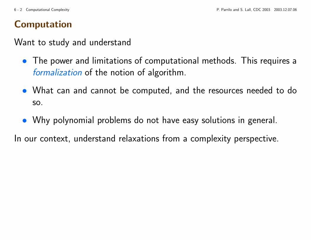
Computation
Want to study and understand
• The power and limitations of computational methods. This requires aformalization of the notion of algorithm.
• What can and cannot be computed, and the resources needed to doso.
• Why polynomial problems do not have easy solutions in general.
In our context, understand relaxations from a complexity perspective.
6 - 3 Computational Complexity P. Parrilo and S. Lall, CDC 2003 2003.12.07.06
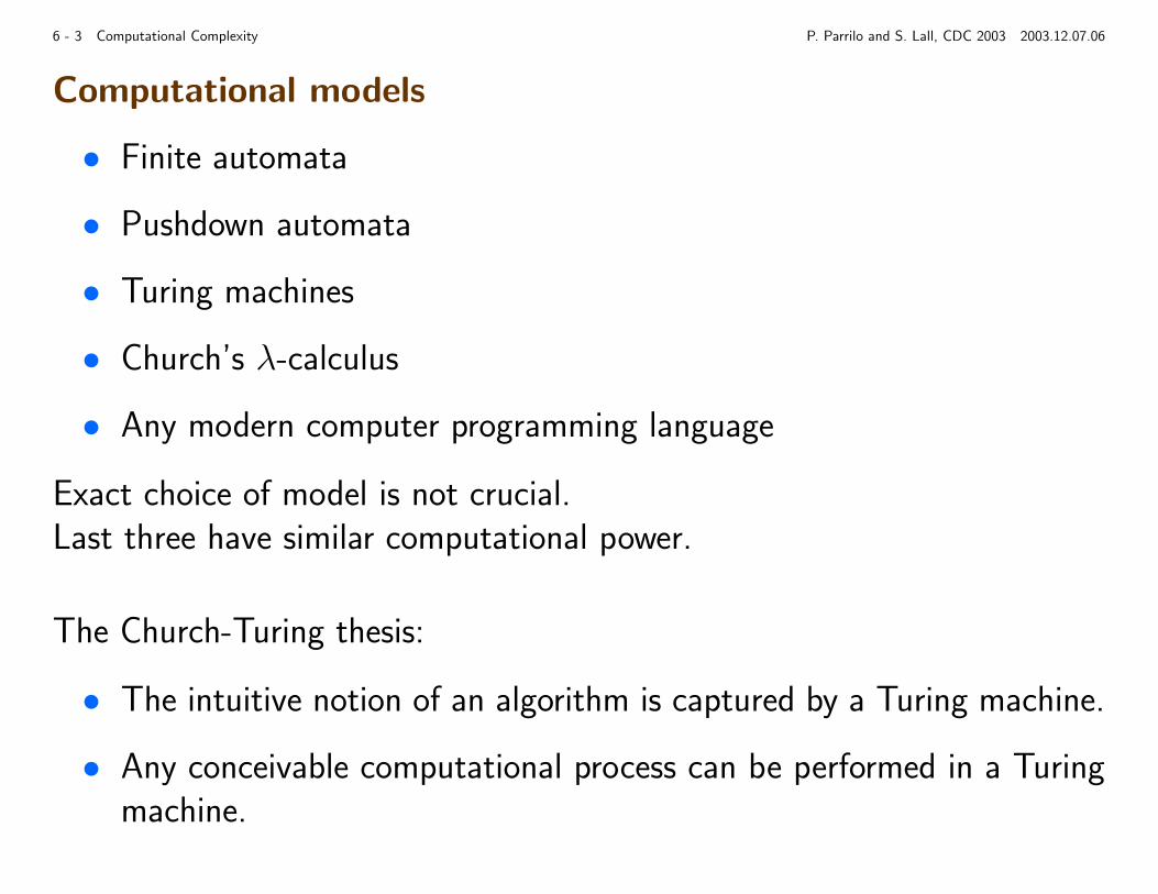
Computational models
• Finite automata
• Pushdown automata
• Turing machines
• Church’s λ-calculus
• Any modern computer programming language
Exact choice of model is not crucial.Last three have similar computational power.
The Church-Turing thesis:
• The intuitive notion of an algorithm is captured by a Turing machine.
• Any conceivable computational process can be performed in a Turingmachine.

6 - 4 Computational Complexity P. Parrilo and S. Lall, CDC 2003 2003.12.07.06
Turing machines
An infinite tape, with a head that moves forwards and backwards.
M
1 0000 01 11
A finite list of rules, that describes the behavior.
Machine reads symbol in tape, moves forward or backwards, and optionallywrites.
• A very idealized abstraction, of purely theoretical use
• This was before computers even existed! (1936)

6 - 5 Computational Complexity P. Parrilo and S. Lall, CDC 2003 2003.12.07.06
A formal notion of computation allows for results on:
• Computability: what can be decided algorithmically?
• A qualitative viewpoint
• Existence of non-algorithmically decidable questions.
• Undecidability of the Turing machine halting problem.
• Application: quadratic integer programming is undecidable.
• Connections with Godel’s incompleteness theorem.
• Complexity: what resources (time, memory, communication) are needed?
• Emphasis on quantitative properties
• Can we solve the problem efficiently?
• Much more recent theory (started in 1970s)

6 - 6 Computational Complexity P. Parrilo and S. Lall, CDC 2003 2003.12.07.06
Decision problems
Complexity classes are defined for decision problems, i.e., those with ayes/no answer.
Examples: Is this graph connected?Is this matrix singular?Is this polynomial nonnegative?Is this proposition satisfiable?Is this optimization problem feasible?
Given a problem, is the answer “Yes” or “No”?
A language is the set of inputs with the desired property.
So we can equivalent ask “Is this instance in the language?”We use “problem” informally, to denote “language”.

6 - 7 Computational Complexity P. Parrilo and S. Lall, CDC 2003 2003.12.07.06
Time complexity
We are interested in the number of operations, as a function of the lengthof the input.
Standard O(·) notation: f (n) is O(g(n)) if there exists a n0 and c > 0such that
n ≥ n0⇒ f (n) ≤ cg(n)
.
Example:(n+5
3
)is O(n3).
For instance, we can say: a Turing machine requires O(n2) units of time,where n is the length of the input.

6 - 8 Computational Complexity P. Parrilo and S. Lall, CDC 2003 2003.12.07.06
Complexity classes: P
P is the class of problems that can be decided in polynomial time, i.e.,those for which the running time is O(nk), for k ∈ N.
Some examples in P:
• Connectedness: Is the graph G connected?
• Nonsingularity: Is the rational matrix M singular?
• Positive semidefiniteness: Is this rational matrix PSD?
• Stability: Is this rational matrix Hurwitz stable?
• Controllability: Is this system controllable?
For all of these, there are algorithms requiring only a polynomial numberof steps.

6 - 9 Computational Complexity P. Parrilo and S. Lall, CDC 2003 2003.12.07.06
Complexity classes: P
Unambiguous and correct decision (yes or no), in polynomial time.
“Efficiently” or “quickly” are synonyms for “in polynomial time”.
If a language is in P, so is its complement.
Ex: If I can efficiently decide “Is this matrix singular?”, then I can alsosolve efficiently “Is this matrix nonsingular?”
Formally, we have that P=coP.

6 - 10 Computational Complexity P. Parrilo and S. Lall, CDC 2003 2003.12.07.06
Complexity classes: NP
NP stands for nondeterministic polynomial time. What does this mean?
Given a “hint”, “guess”, or “certificate”, can verify in polynomial time.
Examples:
• Is this logical proposition satisfiable?If you give me the assignment, it’s easy.
• Compositeness: Is this number composite (not prime)?If you give me the factors, I can multiply them.
• Does this graph have a Hamiltonian path?Given the path, I can easily verify if it is Hamiltonian.
• Is this matrix singular?Give me a vector in the kernel, then I can quickly check.
A “Yes” answer is easy to verify.Can use the certificate as a proof, to quickly convince someone else.
6 - 11 Computational Complexity P. Parrilo and S. Lall, CDC 2003 2003.12.07.06
Complexity classes: NP
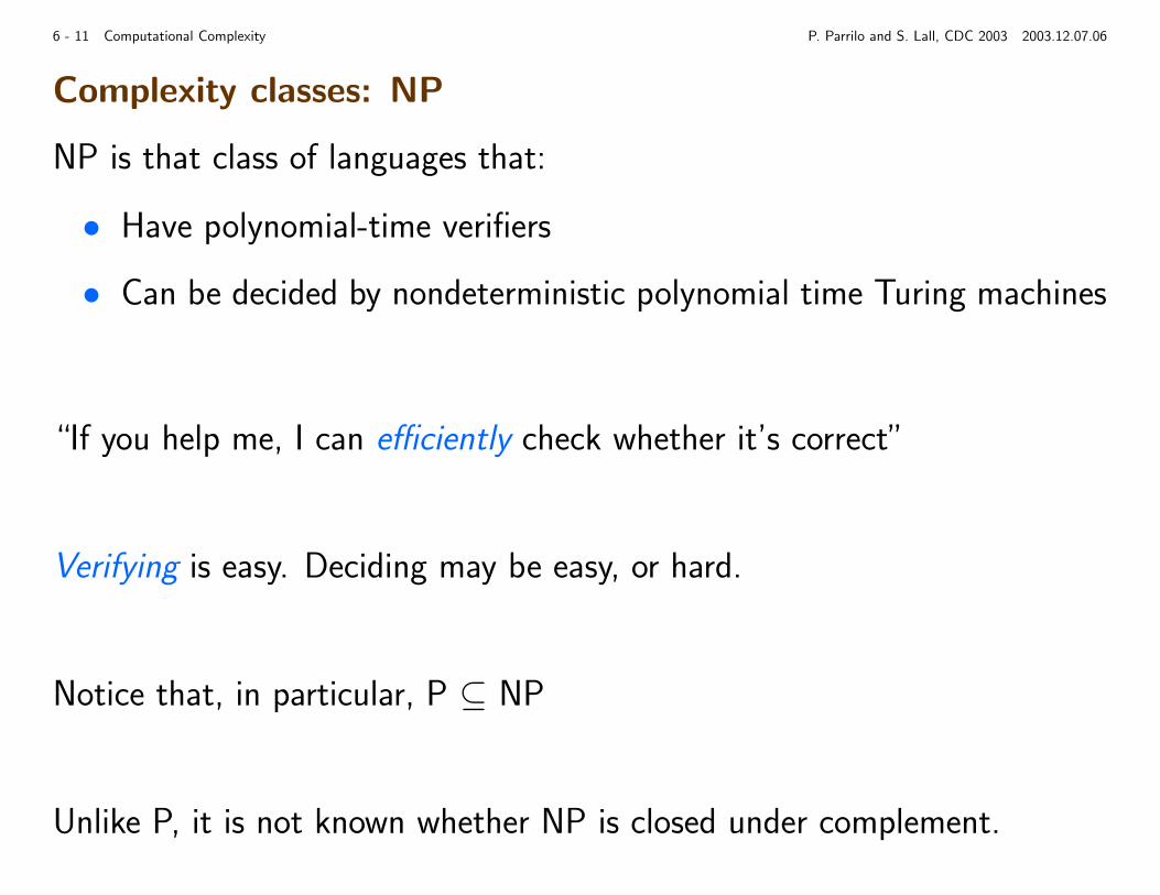
NP is that class of languages that:
• Have polynomial-time verifiers
• Can be decided by nondeterministic polynomial time Turing machines
“If you help me, I can efficiently check whether it’s correct”
Verifying is easy. Deciding may be easy, or hard.
Notice that, in particular, P ⊆ NP
Unlike P, it is not known whether NP is closed under complement.

6 - 12 Computational Complexity P. Parrilo and S. Lall, CDC 2003 2003.12.07.06
Complementation
Consider a logical proposition Q = ¬((p ∧ q)⇒ (q ∧ ¬r)).
For a proposition in n variables,the truth table has 2n rows.
p q r p ∧ q q ∧ ¬r QT T T T F TT T F T T FT F T F F FT F F F F FF T T F F FF T F F T FF F T F F FF F F F F F
To verify that the proposition is satisfiable, it is enough to look at one row.If you tell me which row, I can do that quickly.
However, if it is unsatisfiable, no easy shortcuts in general.For instance, need to look at all 2n rows.

6 - 13 Computational Complexity P. Parrilo and S. Lall, CDC 2003 2003.12.07.06
Complexity classes: coNP
coNP is the set of
• languages for which non-membership can be efficiently verified, witha guess.
• problems that have polynomial-time refutations
• problems for which a “No” answer is easy to verify
• languages whose complement is in NP
Examples:
• Tautologies (propositions that are true for every possible assignment).
• Graphs without Hamiltonian circuits
• Nonnegative functions in [0, 1]n.
6 - 14 Computational Complexity P. Parrilo and S. Lall, CDC 2003 2003.12.07.06
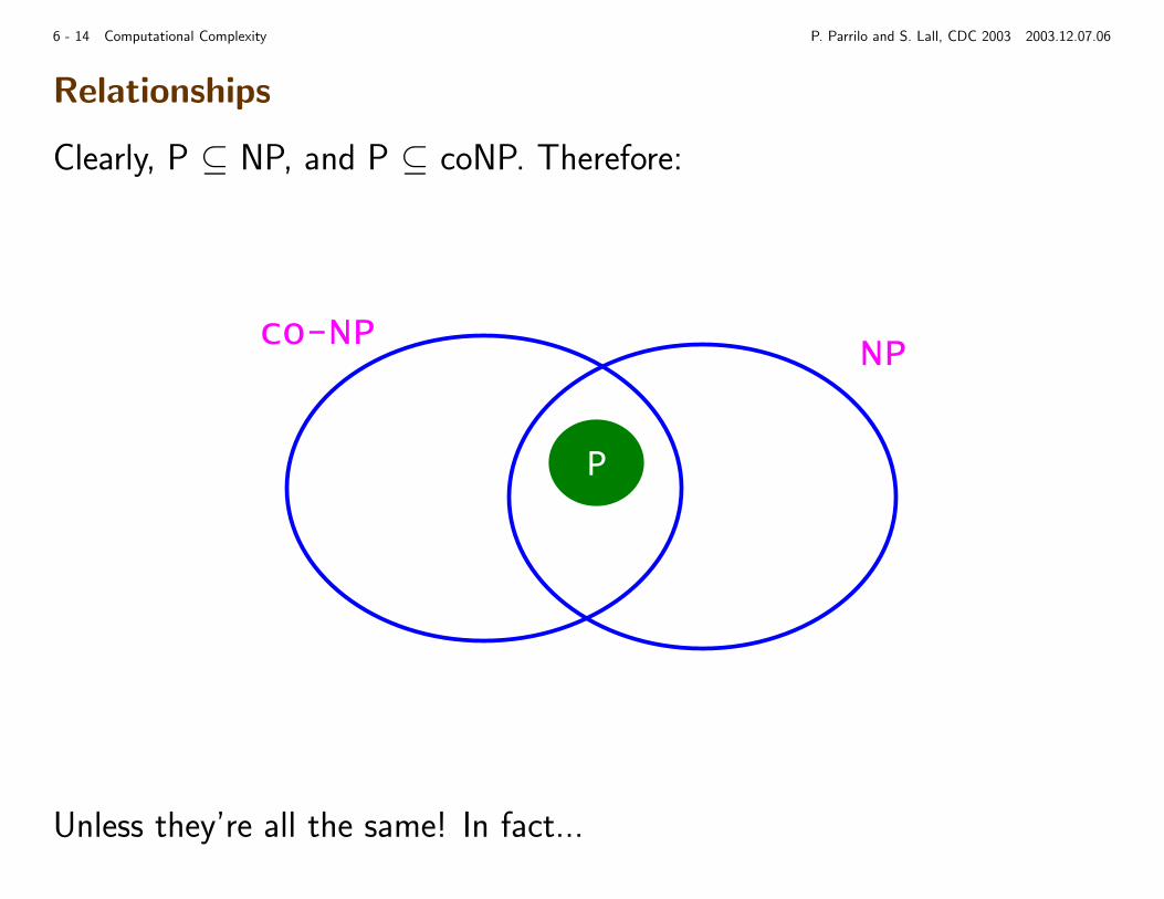
Relationships
Clearly, P ⊆ NP, and P ⊆ coNP. Therefore:
NPco-NP
P
Unless they’re all the same! In fact...

6 - 15 Computational Complexity P. Parrilo and S. Lall, CDC 2003 2003.12.07.06
The big questions
There is a lot that we don’t know:
• Is P=NP?
• Does the existence of a short proof guarantee that we can find itefficiently?
• Is NP=coNP?
• Do all tautologies have short proofs?
• Is it equally easy to certify “yes” and “no” answers?
Have been open for more than 30 years.They’re certainly the most important open questions in theoretical com-puter science, and perhaps in mathematics.
A 1M USD reward from the Clay Institute for a solution.

6 - 16 Computational Complexity P. Parrilo and S. Lall, CDC 2003 2003.12.07.06
Polynomial-time reductions
An important concept: the reducibility of a problem to another.
We transform a problem (language) into another one, not changing signif-icantly the running time.
For instance, we can reduce MAXCUT to a QCQP, efficiently.
If problem A is reducible to B, we write
A ¹P B
The reduction implies that B is “as hard” as A. Since we could use analgorithm for problem B to solve A, it cannot be easier.

6 - 17 Computational Complexity P. Parrilo and S. Lall, CDC 2003 2003.12.07.06
NP-hardness
A problem B is NP-hard if every problem in NP can be reduced to B.
A ∈ NP =⇒ A ¹P B
NP-hard problems are as hard as any problem in NP
• The traveling salesperson problem
• Does this graph have a Hamiltonian path?
• Boolean quadratic optimization
• Satisfiability
• Is the structured singular value µ less than 1?
NP-hard problems are not necessarily in NP.

6 - 18 Computational Complexity P. Parrilo and S. Lall, CDC 2003 2003.12.07.06
NP-completeness
NP-complete = NP ∩ NP-hard
A problem is NP-complete if
• it is in NP
• every other problem in NP is polynomial-time reducible to it.
A nontrivial fact: NP-complete problems exist.
• Satisfiability is NP-complete (Cook-Levin).
• The proof, essentially writing down the equations for a Turing machine.
NP-complete problems are the hardest problems in NP.
6 - 19 Computational Complexity P. Parrilo and S. Lall, CDC 2003 2003.12.07.06
Remarks
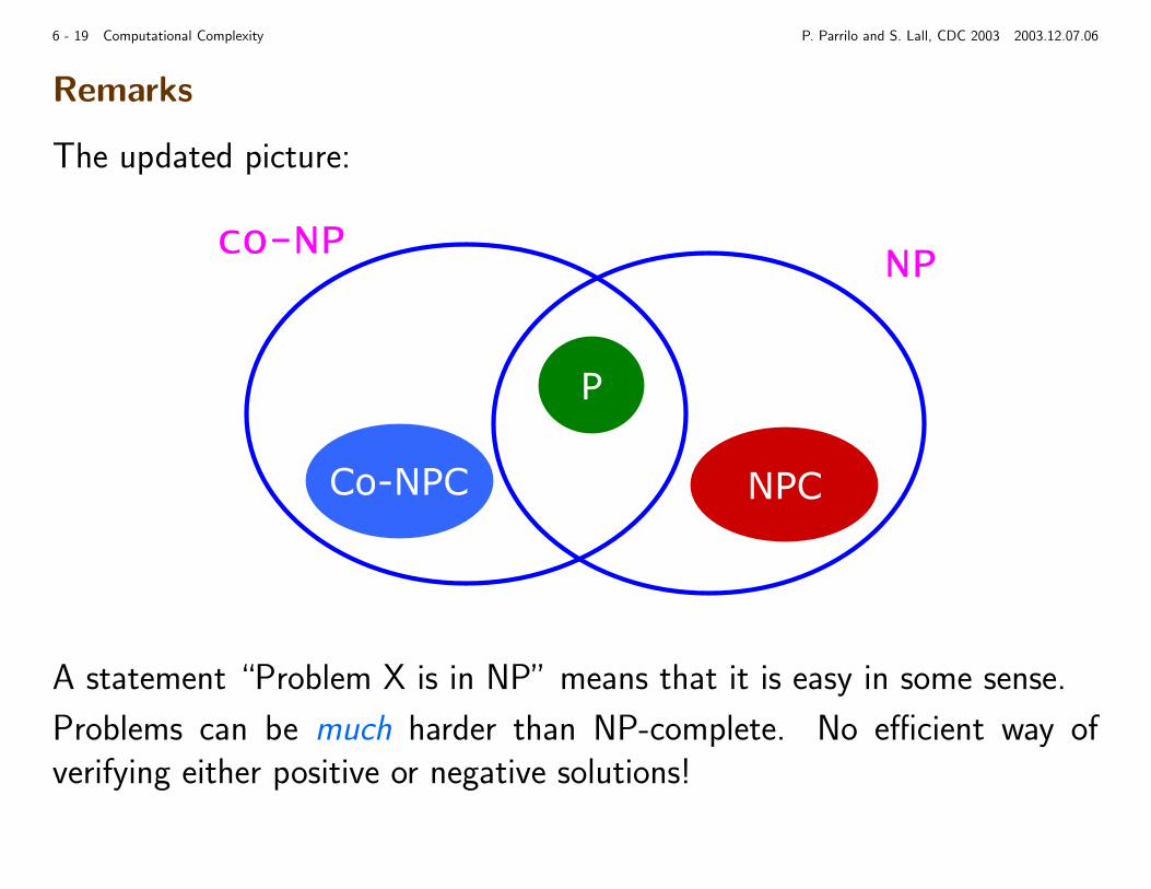
The updated picture:
NPco-NP
P
NPCCo-NPC
A statement “Problem X is in NP” means that it is easy in some sense.
Problems can be much harder than NP-complete. No efficient way ofverifying either positive or negative solutions!

6 - 20 Computational Complexity P. Parrilo and S. Lall, CDC 2003 2003.12.07.06
The famous cartoon
From Garey & Johnson (1979).

6 - 21 Computational Complexity P. Parrilo and S. Lall, CDC 2003 2003.12.07.06
Polynomial feasibility is NP-hard
Sketch: 0-1 linear programming is NP-hard, by reduction from 3SAT.
Using the encoding T ↔ 1, F ↔ 0, we have:
qi ∨ qj ∨ qk is true ⇐⇒ xi + xj + xk ≥ 1.
In other words, we encode logic with arithmetic.
0-1 LP is clearly a special case of polynomial feasibility, since we can writethe 0-1 constraints as x2
i − 1 = 0.
All the required transformations are polynomial time.
So the following holds:
A ∈ NP =⇒ A ¹P 3SAT ¹P 01LP ¹P FEAS
which implies that deciding polynomial feasibility is NP-hard.

6 - 22 Computational Complexity P. Parrilo and S. Lall, CDC 2003 2003.12.07.06
Relativization and the polynomial time hierarchy
What happens if we allow “subroutines” (oracles)?
For instance, if deciding NP-complete problems is “free”?Define Σ0P = Π0P = P, and recursively:
Σk+1P = NP with ΣkP oracle,
Πk+1P = coNP with ΣkP oracle
We have Σ1P = NP, Π1P = coNP. Higherclasses harder.
1Õ
1å
2å
2å
2Õ
3Õ
3å
......
2Õ
3Õ
3å
......
NPCoNP
0 0Õ = å
P
There are problems that are complete for PH: alternating quantifiers.
Ex: (∃x)(∀y)(∃z)Q(x, y, z) is in Σ3P .
These appear in games, minimax, robust control, etc.
Hard to certify solutions, either in the positive or the negative.
If NP=coNP then the polynomial time hierarchy collapses.

6 - 23 Computational Complexity P. Parrilo and S. Lall, CDC 2003 2003.12.07.06
Caveats
Complexity theory admits several variations, according to the specific choices:
Weak vs. strong Computational model Class
Exact problemε-approximation
TuringArithmetic
PNP, coNP
Σk, Πk
For instance, for linear programming feasibility:
• Exact problem, rational data and Turing model, it is in P.
• Exact problem, real arithmetic model, complexity is open.
• Polynomial time in log 1ε for approximate solutions.
6 - 24 Computational Complexity P. Parrilo and S. Lall, CDC 2003 2003.12.07.06
Assessing difficulty
Why do we think of some optimization problems as easy, and others ashard?
“Good” optimization problems:
• LP is polynomial in the Turing model
• Weak LP/SDP are polynomial in the arithmetic real model
“Bad” problems: general polynomial optimization
• NP-hard in the Turing model
• NP-complete in real arithmetic model
Regardless of some important open questions, this classification agrees wellwith practical experience.

6 - 25 Computational Complexity P. Parrilo and S. Lall, CDC 2003 2003.12.07.06
Some positive thoughts
• For practical-sized instances, we may be able to solve problems in anacceptable time.
• Approximate solutions may be easyFor instance, naive coin flipping gives a 1
2 algorithm for MAXCUT.
• But, NP-complete problems differ wildly in approximation properties.MAXCUT is quite nice, CLIQUE cannot be approximated within anyconstant factor.
• Problems may be easy on average, for a given probability distribution.In general, results depend critically on the chosen ensemble
• Classes of instances may admit short proofs.The main idea behind relaxations.
6 - 26 Computational Complexity P. Parrilo and S. Lall, CDC 2003 2003.12.07.06
Relaxations and short proofs
In general, problems in coNP don’t have short proofs (unless NP=coNP).
For a given problem, some instances are easier than others. For any con-crete instance, short proofs may exist, and be easy to find.
Example:
• We do not know how to decide or certify efficiently that a graph doesnot contain a Hamiltonian cycle. If the graph has a bridge, then it iseasy.
• Proving µ(M) < 1 is hard. But, if the SDP upper bound satisfiesµ(M) < 1, we are done.
If NP6=coNP, there exist true propositions for which we cannot conciselyexplain why they’re true!

6 - 27 Computational Complexity P. Parrilo and S. Lall, CDC 2003 2003.12.07.06
A complexity zoo
Different computational models give rise to different complexity classes:
• Working space (memory): PSPACE, EXPSPACE, . . .
• Parallel: NC, PT/WK, . . .
• Randomized versions: PP, BPP, RP, ZPP, . . .
• Real and complex computation: NPR, NPC,. . .
• Approximation and optimization: APX, PTAS, . . .
• Quantum: BQP, . . .
• Enumeration: #P, . . .
• Interactive: IP, MIP, AM, PCP, . . .