DE2-EA 2.1: M4DE Dr Connor Myant

6. 3D Kinematics

Comments and corrections to connor.myant@imperial.ac.uk

Lecture resources may be found on Blackboard and at http://connormyant.com

Contents Three-Dimensional Kinematics and Dynamics of Rigid Bodies ............................................................... 2

Kinematics ............................................................................................................................................... 3

Velocities and Accelerations ............................................................................................................... 3

Moving Reference Frames .................................................................................................................. 4

Euler’s Equations ..................................................................................................................................... 7

Three-Dimensional Kinematics and Dynamics of Rigid Bodies For many engineering applications of complex kinematics and dynamics we must consider three-

dimensional motion. In this chapter we will explain how three-dimensional motion of rigid body is

described. Then we will derive the equations of motion and use them to analyse simple motion.

Design Engineering Example: The ability to model

and understand the motion of the human body

enables better design of garments, wearable tech, and

other products that interface with the consumer

during motion. It is also vital in the medical field as

well; to reach the optimal design of implants and

prosthetics we must first develop methods for

analysing gait and biodynamics. In addition, this

enables clinicians to diagnosing joint conditions,

monitor progression and evaluate treatment

outcomes.

Design Engineering Example: In the near future it is envisaged that aerial robots (Drones) will have

the capability to autonomously construct structures in many applications: building temporary

shelters following natural disasters, deploying scaffolding and support structures on conventional

construction sites, or assembling ramps across gaps and difficult terrain to enable access to

terrestrial vehicles (http://www.imperial.ac.uk/aerialIs/).

In order for such tasks to be carried out

multiple robots will need to be employed

simultaneously. This team of robots will need

to communicate and understand were each

other are, and how they are moving relative to

each other.

Kinematics If a motor bike rides in a straight line, the wheels undergo planar motion. But, if the bike is turning the

motion of the wheels is three dimensional (Figure 6.1). The same can be said for an aeroplane; planar

motion when in level flight, 3D when banking or turning. A spinning top will be in planar motion at

first, rotating about a fixed vertical axis. But, will eventually begin to tilt and rotate under 3D motion.

Figure 6.1. Example of planar and three-dimensional motion

Velocities and Accelerations We have already looked at the basic concepts needed to describe the 3D motion of rigid bodies

relative to a given reference frame. In the earlier chapters on Kinematics we showed that a rigid body

undergoing any motion other than translation has an instantaneous axis of rotation. The direction of

this axis at a particular instant and the rate at which the rigid body rotates about the axis are specified

by the angular velocity vector �⃑⃑⃑� .

We have also shown that a rigid body’s velocity is completely specified by its angular velocity vector

and the velocity of a single point of the body. For the rigid body and reference frame in Figure 6.2,

suppose we know the angular velocity vector �⃑⃑⃑� and the velocity 𝑣𝐵 of a point 𝐵. Then the velocity of

any other point 𝐴 of the body is given by;

𝑣𝐴 = 𝑣𝐵 + �⃑⃑⃑� × 𝑟𝐴/𝐵 (6.1)

A rigid body’s acceleration is completely specified by its angular acceleration vector �⃑⃑� =𝑑�⃑⃑⃑�

𝑑𝑡, its

angular velocity vector, and the acceleration of a single point of the body. If we know �⃑⃑� and �⃑⃑⃑� and

the acceleration 𝑎𝐵 of the point 𝐵, the acceleration of any other point 𝐴 of the rigid body is given by;

𝑎𝐴 = 𝑎𝐵 + �⃑⃑� × 𝑟𝐴/𝐵 + �⃑⃑⃑� × (�⃑⃑⃑� × 𝑟𝐴/𝐵) (6.2)

Figure 6.2. Points A and B of a rigid body. The velocity of A can be determined if the velocity of B and

the rigid body’s angular velocity vector ω are known. The acceleration of A can be determined if the

acceleration of B, the angular velocity vector, and the angular acceleration vector are known.

Moving Reference Frames

The velocities and accelerations in Equations (6.1) and (6.2) are measured relative to the reference

frame indicated in Figure 6.2, which we will refer to as the primary reference frame (normally fixed

relative to the earth). We also use a secondary reference frame that moves relative to the primary

reference frame. The secondary reference frame and its motion are chosen for convenience in

describing the motion of a particular rigid body. In some situation, the secondary reference frame is

defined to be fixed with respect to the rigid body. In other cases, it is advantageous to use a secondary

reference frame that moves relative to the primary reference frame, but is not fixed with respect to

the rigid body.

Figure 6.3 shows a primary reference frame, a secondary reference frame 𝑥𝑦𝑧, and a rigid body. The

angular velocity of the secondary reference frame is specified by the vector �⃑⃑� , and the angular velocity

of the rigid body relative to the primary reference frame is specified by the vector �⃑⃑⃑� . A third

component is �⃑⃑⃑� 𝑟𝑒𝑙, which is the angular velocity vector of the rigid body relative to the secondary

reference frame.

When the secondary reference frame is not fixed to the rigid body, we can express the body’s angular

velocity vector �⃑⃑⃑� as the sum of the angular velocity vector �⃑⃑� of the secondary reference frame and

the angular velocity vector �⃑⃑⃑� 𝑟𝑒𝑙 of the rigid body relative to the secondary reference frame;

�⃑⃑⃑� = �⃑⃑� + �⃑⃑⃑� 𝑟𝑒𝑙 (6.3)

Figure 6.3. The primary and secondary reference frames. The vector �⃑⃑� is the angular velocity of the

secondary reference frame relative to the primary reference frame. The vector �⃑⃑⃑� is the angular

velocity of the rigid body relative to primary reference frame.

The rigid body’s angular acceleration vector relative to the primary reference frame can then be

expressed as;

�⃑⃑� =𝑑�⃑⃑⃑�

𝑑𝑡=

𝒅�⃑⃑�

𝒅𝒕+

𝒅�⃑⃑⃑� 𝑟𝑒𝑙

𝒅𝒕= (

𝒅�⃑⃑⃑� 𝑟𝑒𝑙

𝒅𝒕+ �⃑⃑� × �⃑⃑⃑� 𝑟𝑒𝑙) + (

𝒅�⃑⃑� 𝑟𝑒𝑙

𝒅𝒕+ �⃑⃑� × �⃑⃑� ) (6.4)

The right hand side of this equation becomes zeros, leaving;

�⃑⃑� =𝒅�⃑⃑⃑� 𝑟𝑒𝑙

𝒅𝒕+ �⃑⃑� × �⃑⃑⃑� 𝑟𝑒𝑙 (6.5)

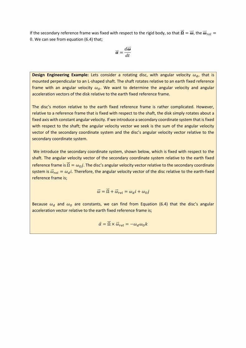
If the secondary reference frame was fixed with respect to the rigid body, so that �⃑⃑� = �⃑⃑⃑� , the �⃑⃑⃑� 𝑟𝑒𝑙 =

0. We can see from equation (6.4) that;

�⃑⃑� =𝑑�⃑⃑⃑�

𝑑𝑡

Design Engineering Example: Lets consider a rotating disc, with angular velocity 𝜔𝑑, that is

mounted perpendicular to an L-shaped shaft. The shaft rotates relative to an earth fixed reference

frame with an angular velocity 𝜔𝑂. We want to determine the angular velocity and angular

acceleration vectors of the disk relative to the earth fixed reference frame.

The disc’s motion relative to the earth fixed reference frame is rather complicated. However,

relative to a reference frame that is fixed with respect to the shaft, the disk simply rotates about a

fixed axis with constant angular velocity. If we introduce a secondary coordinate system that is fixed

with respect to the shaft; the angular velocity vector we seek is the sum of the angular velocity

vector of the secondary coordinate system and the disc’s angular velocity vector relative to the

secondary coordinate system.

We introduce the secondary coordinate system, shown below, which is fixed with respect to the

shaft. The angular velocity vector of the secondary coordinate system relative to the earth fixed

reference frame is Ω⃑⃑ = 𝜔𝑂𝑗. The disc’s angular velocity vector relative to the secondary coordinate

system is �⃑⃑� 𝑟𝑒𝑙 = 𝜔𝑑𝑖. Therefore, the angular velocity vector of the disc relative to the earth-fixed

reference frame is;

�⃑⃑� = Ω⃑⃑ + �⃑⃑� 𝑟𝑒𝑙 = 𝜔𝑑𝑖 + 𝜔𝑂𝑗

Because 𝜔𝑑 and 𝜔𝑂 are constants, we can find from Equation (6.4) that the disc’s angular

acceleration vector relative to the earth fixed reference frame is;

𝛼 = Ω⃑⃑ × �⃑⃑� 𝑟𝑒𝑙 = −𝜔𝑑𝜔𝑂𝑘

You will pick up 3D kinematics again in Robotics 1 next year.

THE NEXT SECTION IS OPTION AND WILL NOT BE INCLUDED IN THE EXAM!

Euler’s Equations To complete the kinematics and dynamics ‘loop’ I have included the following optional section.

In classical mechanics, Euler's rotation equations are a vectorial quasilinear first-order ordinary

differential equation describing the rotation of a rigid body, using a rotating reference frame with its

axes fixed to the body and parallel to the body's principal axes of inertia.

So in basic term we are using the technique we just employed to study the kinematics of a moving

reference frame and adding mass so that it becomes a dynamics problem. But only for cases where

the secondary reference frame is body fixed to the body in question and parallel to the body’s principal

axes of inertia.

Recap: From Dynamics we know that the moment of inertia of a rigid body is a tensor* that

determines the torque needed for a desired angular acceleration about a rotational axis. It depends

on the body's mass distribution and the axis chosen, with larger moments requiring more torque to

change the body's rotation. It is an extensive (additive) property: For a point mass the moment of

inertia is just the mass times the square of perpendicular distance to the rotation axis. The moment

of inertia of a rigid composite system is the sum of the moments of inertia of its component

subsystems (all taken about the same axis).

Euler's equations consist of Newton’s second law; ∑𝐹 = 𝑚𝑎. Which states that the sum of the

external forces on a rigid body equals the product of its mass and the acceleration of its centre of

mass, and equations of angular motion. Previously in 2D dynamics we showed how this related to

equation of angular motion; ∑𝑀𝑂 = 𝐼𝑂𝛼, for an object in rotation and ∑𝑀 = 𝐼𝛼 for an object in

planar motion.

Now that we want to introduce 3D motion we need to consider additional reference systems. Here is

where the Euler equations come in. They essentially combine (6.5) into the equations of angular

motion. The generalised form is given as:

Σ𝑀 = 𝐼𝑑�⃑⃑⃑�

𝑑𝑡+ Ω⃑⃑ × (𝐼�⃑⃑� ) (6.6)

Tensor: In mathematics, tensors are geometric objects that describe linear relations between

geometric vectors, scalars, and other tensors. Examples of such relations include the dot product,

the cross product, and linear maps. We will be exploring tensors and tensor matrices more in stress

analysis.

The Inertia Tensor can be expressed in a matric as;

𝐼 = [

𝐼𝑥𝑥 −𝐼𝑥𝑦 −𝐼𝑥𝑧

−𝐼𝑦𝑥 𝐼𝑦𝑦 −𝐼𝑦𝑧

−𝐼𝑧𝑥 −𝐼𝑧𝑦 𝐼𝑧𝑧

]

Which can be visualised on a cube element as shown in figure 6.4.

Figure 6.4. Inertia tensors acting on a cube element. With the origin of the 𝑋𝑌𝑍 axes at the centre

of mass of the cube.

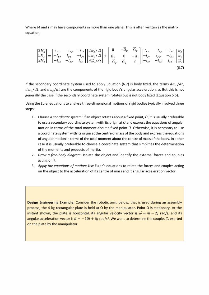
Where 𝑀 and 𝐼 may have components in more than one plane. This is often written as the matrix

equation;

[

Σ𝑀𝑥

Σ𝑀𝑦

Σ𝑀𝑧

] = [

𝐼𝑥𝑥 −𝐼𝑥𝑦 −𝐼𝑥𝑧

−𝐼𝑦𝑥 𝐼𝑦𝑦 −𝐼𝑦𝑧

−𝐼𝑧𝑥 −𝐼𝑧𝑦 𝐼𝑧𝑧

] [

𝑑�⃑⃑� 𝑥 𝑑𝑡⁄

𝑑�⃑⃑� 𝑦 𝑑𝑡⁄

𝑑�⃑⃑� 𝑧 𝑑𝑡⁄

] + [

0 −Ω⃑⃑ 𝑧 Ω⃑⃑ 𝑦

Ω⃑⃑ 𝑧 0 −Ω⃑⃑ 𝑥

−Ω⃑⃑ 𝑦 Ω⃑⃑ 𝑥 0

] [

𝐼𝑥𝑥 −𝐼𝑥𝑦 −𝐼𝑥𝑧

−𝐼𝑦𝑥 𝐼𝑦𝑦 −𝐼𝑦𝑧

−𝐼𝑧𝑥 −𝐼𝑧𝑦 𝐼𝑧𝑧

] [

�⃑⃑� 𝑥�⃑⃑� 𝑦�⃑⃑� 𝑧

]

(6.7)

If the secondary coordinate system used to apply Equation (6.7) is body fixed, the terms 𝑑𝜔𝑥 𝑑𝑡⁄ ,

𝑑𝜔𝑦 𝑑𝑡⁄ , and 𝑑𝜔𝑧 𝑑𝑡⁄ are the components of the rigid body’s angular acceleration, 𝛼. But this is not

generally the case if the secondary coordinate system rotates but is not body fixed (Equation 6.5).

Using the Euler equations to analyse three-dimensional motions of rigid bodies typically involved three

steps:

1. Choose a coordinate system: If an object rotates about a fixed point, 𝑂, it is usually preferable

to use a secondary coordinate system with its origin at 𝑂 and express the equations of angular

motion in terms of the total moment about a fixed point 𝑂. Otherwise, it is necessary to use

a coordinate system with its origin at the centre of mass of the body and express the equations

of angular motion in terms of the total moment about the centre of mass of the body. In either

case it is usually preferable to choose a coordinate system that simplifies the determination

of the moments and products of inertia.

2. Draw a free-body diagram: Isolate the object and identify the external forces and couples

acting on it.

3. Apply the equations of motion: Use Euler’s equations to relate the forces and couples acting

on the object to the acceleration of its centre of mass and it angular acceleration vector.

Design Engineering Example: Consider the robotic arm, below, that is used during an assembly

process; the 4 kg rectangular plate is held at O by the manipulator. Point O is stationary. At the

instant shown, the plate is horizontal, its angular velocity vector is �⃑⃑� = 4𝑖 − 2𝑗 rad/s, and its

angular acceleration vector is 𝛼 = −10𝑖 + 6𝑗 rad/s2. We want to determine the couple, 𝐶, exerted

on the plate by the manipulator.

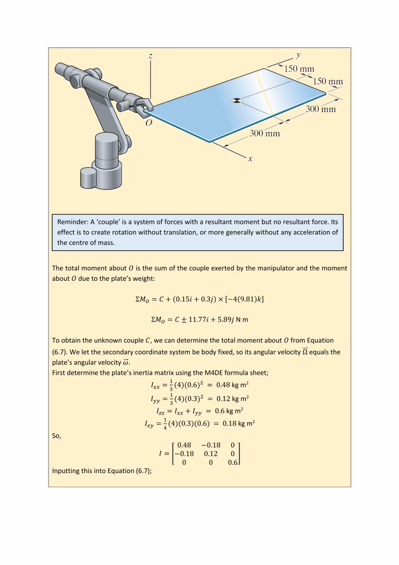
The total moment about 𝑂 is the sum of the couple exerted by the manipulator and the moment

about 𝑂 due to the plate’s weight:

Σ𝑀𝑂 = 𝐶 + (0.15𝑖 + 0.3𝑗) × [−4(9.81)𝑘]

Σ𝑀𝑂 = 𝐶 ± 11.77𝑖 + 5.89𝑗 N m

To obtain the unknown couple 𝐶, we can determine the total moment about 𝑂 from Equation

(6.7). We let the secondary coordinate system be body fixed, so its angular velocity Ω⃑⃑ equals the

plate’s angular velocity �⃑⃑� .

First determine the plate’s inertia matrix using the M4DE formula sheet;

𝐼𝑥𝑥 =1

3(4)(0.6)2 = 0.48 kg m2

𝐼𝑦𝑦 =1

3(4)(0.3)2 = 0.12 kg m2

𝐼𝑧𝑧 = 𝐼𝑥𝑥 + 𝐼𝑦𝑦 = 0.6 kg m2

𝐼𝑥𝑦 =1

4(4)(0.3)(0.6) = 0.18 kg m2

So,

𝐼 = [0.48 −0.18 0

−0.18 0.12 00 0 0.6

]

Inputting this into Equation (6.7);

Reminder: A ‘couple’ is a system of forces with a resultant moment but no resultant force. Its

effect is to create rotation without translation, or more generally without any acceleration of

the centre of mass.

[

Σ𝑀𝑥

Σ𝑀𝑦

Σ𝑀𝑧

] = [0.48 −0.18 0

−0.18 0.12 00 0 0.6

] [−1060

] + [0 0 −20 0 −42 4 0

] [0.48 −0.18 0

−0.18 0.12 00 0 0.6

] [4

−20

]

[

Σ𝑀𝑥

Σ𝑀𝑦

Σ𝑀𝑧

] = [−5.882.520.72

] N m

We substitute into the above equation for;

Σ𝑀𝑂 = 𝐶 ± 11.77𝑖 + 5.89𝑗 = −5.88i + 2.52j + 0.72k

And solve for 𝐶;

𝐶 = 5.89𝑖 − 3.37𝑗 + 0.72𝑘 N m