6 0066.006- Idi AlihIntroduction to Algorithms · ItIts’sthecallstackofthepythoninterpreter the call stack of the python interpreter From v, recurse on one child at a time ... Axe

6 006 I d i Al i h6.006- Introduction to Algorithms

Lecture 13Prof Manolis KellisProf. Manolis Kellis

CLRS 22.4-22.5

Goal for today: Graphs III• Recap on graphs, games, searching, BFS

Defs Rubik BFS correctness shortest paths– Defs, Rubik, BFS, correctness, shortest paths• Depth first search (DFS). DFS vs. BFS

– Algorithm, runtime, correctness, edge classes• Applications of DFSpp f

– Topological Sort on DAGs, job schedulingConnected components strongly connected– Connected components, strongly connected

• Properties of real-world & biological networks– Types, small-world, scale-free, growth, motifs,

interpreting, centrality, similarity, dynamics

Graphs• G=(V,E)• V a set of verticesp

Usually number denoted by n

• E V ´ V a set of edges (pairs of vertices)U ll b d d b Usually number denoted by m

Note m ≤ n(n-1) = O(n2)

a b a

Undirected example Directed example

• V={a,b,c,d}• V = {a b c}

c d b c

• E={{a,b}, {a,c}, {b,c}, {b,d}, {c,d}}

• V = {a,b,c}• E = {(a,c), (a,b) (b,c), (c,b)}

Searching for a solution pathSearching for a solution path

1 t

6 neighbors27 two-away

1 turn

How big is the space?g p

• Graph algorithms allow us explore space– Nodes: configurations– Edges: moves between themg– Paths to ‘solved’ configuration: solutions

BFS algorithm outlineI iti l t• Initial vertex s– Level 0

• For i=1 v• For i=1,… grow level i– Find all neighbors of level i-1 sg– (except those already seen)– i.e. level i contains vertices

h bl i th f i dLevel 3

reachable via a path of i edges and no fewer

• Where can the other edges of the graph be?Level 1Level 2Where can the other edges of the graph be?

– They cannot jump a layer (otherwise v would be in Level 2)

h b b d i dj

Level 1

– But they can be between nodes in same or adjacent levels

BFS Algorithm

• BFS(V,Adj,s)l l { 0} t { N } i 1level={s: 0}; parent = {s: None}; i=1frontier=[s] #previous level, i-1while frontierwhile frontier

next=[] #next level, ifor u in frontier

for v in Adj[u]if v not in level #not yet seen

level[v] = i #level of u+1level[v] = i #level of u+1parent[v] = unext.append(v)

frontier = nexti += 1

BFS Analysis: Correctnessi e why are all nodes reachable from s explored?

• Claim: If there is a path of L edges from s to v

i.e. why are all nodes reachable from s explored?(we’ll actually prove a stronger claim)

Claim: If there is a path of L edges from s to v, then v is added to next when i=L or before

• Proof: induction L‐1 L

u

L‐1

Base case: s is added before setting i=1 Inductive step when i=L:

• Consider path of length L from s to v

(…)

uv

s

• Consider path of length L from s to v• This must contain: (1) a path of length L-1 from s to u• (2) and an edge (u,v) from u to v

B i d ti h th i dd d t t By inductive hypothesis, u was added to next when i=L-1 or before

• If v has not already been inserted in next before i=L, then it gets added during the scan of Adj[u] at i=Lthen it gets added during the scan of Adj[u] at i=L

So it happens when i=L or before. QED

Corrollary: BFSShortest PathsCorrollary: BFSShortest Paths• From correctness analysis, conclude more:

L l[ ] i l h f h h Level[v] is length of shortest sv path• Parent pointers form a shortest paths tree i.e. the union of shortest paths to all vertices

• To find shortest path from s to vp Follow parent pointers from v backwards Will end up at sp

a s d f1 2

30

a

z

d f

Shortest paths tree

c vxz 12

2 3 v

sx c

BFS







Depth First Search (DFS)Depth First Search (DFS)

DFS Algorithm OutlineDFS Algorithm Outline• Explore a mazep Follow path until you get stuck Backtrack along breadcrumbs till find new exitg i.e. recursively explore

DFS AlgorithmDFS Algorithm

• parent = {s: None}parent {s: None}• call DFS-visit (V, Adj, s)

def DFS-visit (V, Adj, u)for v in Adj[u]

if v not in parent #not yet seenp yparent[v] = uDFS visit (V Adj v) #recurse!DFS-visit (V, Adj, v) #recurse!

DFS example run (starting from s)

s 1 (in tree)s ( )

2 (

5 (for

a

in tree)

rward ed

3 (in tree)

dge)

bc 7 ( d )c

ab c

7 (cross edge)d

s

a

d

DFS Runtime AnalysisDFS Runtime Analysis• Quite similar to BFSQ• DFS-visit only called once per vertex v Since next time v is in parent setSince next time v is in parent set

• Edge list of v scanned only once (in that call)S ti i DFS i it i• So time in DFS-visit is: 1 per vertex + 1 per edge

• So time is O(n+m)

DFS Correctness?DFS Correctness?• Trickier than BFS• Can use induction on length of shortest path from

starting vertexg Inductive Hypothesis:

“each vertex at distance k is visited (eventually)” Induction Step:

• Suppose vertex v at distance k. Then some u at shortest distance k 1 with edge (u v) Then some u at shortest distance k-1 with edge (u,v) Can decompose into su at shortest distance k-1, and (u,v)

• By inductive hypothesis: u is visited (eventually)• By algorithm: every edge out of u is checked

If v wasn’t previously visited, it gets visited from u (eventually)

Edge ClassificationEdge Classification

• Tree edge used to get to new childTree edge used to get to new child• Back edge leads from node to ancestor in tree• Forward edge leads to descendant in tree• Forward edge leads to descendant in tree• Cross edge leads to a different subtree

T l b l h t d i f h t t k l b l• To label what edge is of what type, keep global time counter and store interval during which vertex is on recursion stackvertex is on recursion stack

tree edge

Cross edge Forward edgeBack edge







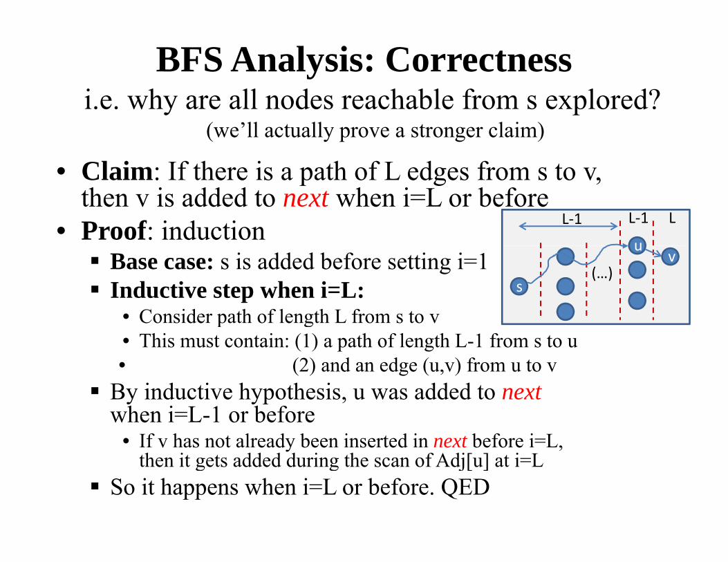
BFS vs DFSBFS vs. DFS

Breadth First SearchBreadth First Search• start with vertex v list all its neighbors (dist 1)list all its neighbors (dist 1) then all their neighbors (distance 2)

• Define frontier {s}{dist1}{dist2}{ } { } { }• Repeat until all vertices found

D th Fi t S hDepth First Search• Like exploring a maze• From current vertex, move to another• Until you get stuck• Then backtrack till new place to explore

BFS/DFS Algorithm SimilaritiesBFS/DFS Algorithm Similarities• Maintain “todo list” of vertices to be scanned

• Until list is emptyUntil list is empty Take a vertex v from front of list Mark it scanned Mark it scanned Examine all outgoing edges (v,u)

If t k d dd t th t d li t If u not marked, add to the todo list• BFS: add to end of todo list • DFS: add to front of todo list

(queue: FIFO)(recursion stack: LIFO)• DFS: add to front of todo list (recursion stack: LIFO)

Key difference: Queue vs. StackKey difference: Queue vs. Stack• BFS queue is explicit Created in pieces (level 0 vertices) . (level 1 vertices) . (level 2

vert… the frontier at iteration i is piece i of vertices in

queuequeue• DFS stack is implicit It’s the call stack of the python interpreter It s the call stack of the python interpreter From v, recurse on one child at a time But same order if put all children on stack then But same order if put all children on stack, then

pull off (and recurse) one at a time







Topological SortTopological Sort

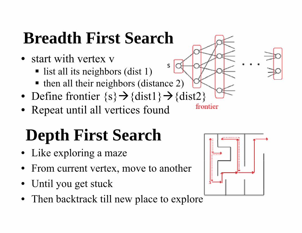
Job SchedulingJob Scheduling• Given A set of tasks Precedence constraints

• saying “u must be done before v”

Represented as a directed graphp g p• Goal: Find an ordering of the tasks that satisfies allFind an ordering of the tasks that satisfies all

precedence constraints

k b i

Scheduling a set of jobsFall out of bedMake bus in

seconds flat

Look up (at clock)

Drag a comb across my head

Notice that

Find my coatNotice that

I’m late Drink a cup

Wake up

Find my way d

Wake up

Grab my hatdownstairs

y

Wake upFall out of bed2 1

Defining job ordering constraintsWake up


Fall out of bed

3

2

Find my way downstairs4

Look upDrink a cup

65

Notice I’m late8 late

Grab my hat

Find my coat 9

87

Make the bus in seconds flat 10

Feasibility / schedule existenceI th h d l ?• Is there a schedule?

Fix hole in bucket

Fetch W t

Cut tWater straw

h Sharpen Axe

Whet Stone

• Each requires previous one to be completed first

Directed Acyclic Graphs (DAGs)y p ( )• Directed Acyclic Graph

G h i h l A h d l i ! Graph with no cycles A schedule exists!• Source: vertex with no incoming edges• Claim: every DAG has a source Start anywhere, follow edges backwardsy , g If never get stuck, must repeat vertex So, get stuck at a source, g

• Conclude: every DAG has a schedule Find a source it can go first Find a source, it can go first Remove, schedule rest of work recursively

Scheduling algorithm 1 (for DAGs)• Find a source Scan vertices to find one with no incoming edges Or use DFS on backwards graph

• Remove, recurseRemove, recurse• Time to find one source O(m) with standard adjacency list representation O(m) with standard adjacency list representation Scan all edges, count occurrence of every vertex

as tailas tail• Total: O(nm)

Scheduling algorithm 2 (for DAGs)g g ( )

• Consider DFS• Observe that we don’t return from recursive call

to DFS(v) until all of v’s children are finishedto DFS(v) until all of v s children are finished• So, “finish time” of v is later than finish time of

all childrenall children• Thus, later than finish time of all descendants

i i h bl f i.e., vertices reachable from v Descendants well-defined since no cycles

• So, reverse of finish times is valid schedule

Implementation of scheduling alg 2• seen = {}; finishes = {}; time = 0

DFS-visit (s)S v s (s)for v in Adj[s]

if v not in seen

only set finishes if

seen[v] = 1 DFS-visit (v) only set finishes if

done processing all edges leaving v

time = time+1finishes[v] = time

• TopologicalSortfor s in V

DFS-visit(s)• Sort vertices by finishes[] key

Wake upFall out of bed10

9


8

Find my way d t i

y

7

Look upDrink a cup

downstairs

45

Notice I’m

Look up (at clock)

Find my coat

2

late

Grab my hat

coat

63In progress

Make bus in seconds flat

y

1Completed

AnalysisAnalysis• Just like connected components DFSp Time to DFS-Visit from all vertices is O(m+n) Because we do nothing with already seen verticesg y

• Might DFS-visit a vertex v before its ancestor u i e start in middle of graph i.e., start in middle of graph Does this matter? No because finish[v] < finish[u] in that case No, because finish[v] < finish[u] in that case

Handling Cyclesg y• If two jobs can reach each other, we must do

h ithem at same time• Two vertices are strongly connected if each

can reach the other • Strongly connected is an equivalence relationg y q So graph has strongly connected components

• Can we find them?Can we find them? Yes, another nice application of DFS But tricky (see CLRS) But tricky (see CLRS) You should understand algorithm, not proof


Defs Rubik BFS correctness shortest paths– Defs, Rubik, BFS, correctness, shortest paths• Depth first search (DFS).





Connected ComponentsConnected Components

Connected ComponentsConnected Components• Undirected graph G=(V,E)g p ( )• Two vertices are connected if there is a path

between thembetween them• An equivalence relation

E i l l ll d t• Equivalence classes are called components A set of vertices all connected to each other

Finding all connected componentsTo find one connected component: • The key idea: Both DFS and BFS will reach all y

vertices reachable from starting vertex s i.e., the ‘component’ of any starting vertex s

• Start with any vertex s: Run DFS (or BFS) to find all vertices in component Mark them as belonging to the same component as s

To find all connected components: • Run the above search n times Starting with every vertex

Naïve Algorithm: DFS n times• DFS-visit (u, owner, o)

#mark all nodes reachable from u with owner ofor v in Adj[u]

if v not in owner #not yet seenowner[v] = o #instead of parentowner[v] o #instead of parentDFS-visit (v, owner, o)

• DFS-Visit(s, owner, s) will mark owner[v]=s f h bl ffor any vertex reachable from s

• Correctness:• Correctness: All vertices in same component will receive the same

ownership labels• Cost? n times BFS/DFS? O(n(m+n))?

Better: DFS only for unmarked verticesy• If vertex has already been reached, don’t need to

h f it!search from it! Its connected component already marked with owner

• owner = {} # global variable ownerowner {} # global variable ownerfor s in V

if not(s in owner)DFS Visit(s owner s) #or can use BFSDFS-Visit(s, owner, s) #or can use BFS

• Now every vertex examined exactly twice Once in outer loop and once in DFS-VisitOnce in outer loop and once in DFS Visit

• And every edge examined once In DFS-Visit when its tail vertex is examined

• Total runtime to find components is O(m+n)

Directed GraphsDirected Graphs• In undirected graphs, connected components g p p

can be represented in n space One “owner label” per vertexp

• Can ask to compute all vertices reachable from each vertex in a directed grapheach vertex in a directed graph i.e. the “transitive closure” of the graph Answer can be different for each vertex Answer can be different for each vertex Explicit representation may be bigger than graph E g size n graph with size n2 transitive closure E.g. size n graph with size n2 transitive closure







Global properties of networksGlobal properties of networks

Mostly pointers for further reading

Networks in the real world

• Infrastructure: Internet, power, transport, distributionf , p , p ,• Social: friends, actors, co-authors, affiliation members• Information: web pages, paper citations, patents,

file-sharing, shopping lists, document-keyword• Biology: physical, metabolic, regulatory, neural, ecological

Properties of real-world networksS ll ld Mil 6 d (’60 )• Small-world property: Milgram 6-degrees (’60s) Any pair of vertices connected by short paths People find these paths with no global information People find these paths with no global information

• ‘Scale-free’/power-law degree distribution: 80/20 rule: 80% of connections in 20% of vertices 80/20 rule: 80% of connections in 20% of vertices Few heavily-connected hubs, most lie in the fringes

• Network growth and preferential attachmentNetwork growth and preferential attachment Rich-get-richer can lead to power-law distributions

• Clustering coefficient: average probability that v’sCluste ing coefficient: ave age p obab ty t at v sneighbors are also connected to each other. Measures the density of closed vs. open ‘triangles’ More generally: measure frequency of all network motifs,

i.e. over-/under-representation of all sub-graphs size 3,4,5,…

Network ‘motifs’_• Network building blocks Smallest meaningful unitg

• Interpretable circuit componentscomponents Feed-forward loops Feedback loopsFeedback loops Cross-regulation Amplification etc Amplification, etc

• Discovered based on th i t titheir over-representation Compared to ‘random’ net

Interpreting biological network properties• Hierarchical organization• Hierarchical organization Master regulators vs. local regulators

D di t ib ti• Degree distribution In-hubs, out-hubs

Di t• Diameter Info transfer

M d l i• Modularity Locality

• Clustering Subnetworks

• Flow direction Downward/upward e.g. modENCODE consortium, Science, 2010

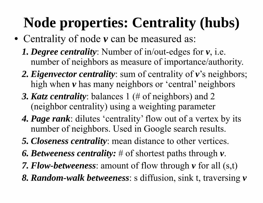
Node properties: Centrality (hubs)• Centrality of node v can be measured as:• Centrality of node v can be measured as:

1. Degree centrality: Number of in/out-edges for v, i.e. number of neighbors as measure of importance/authoritynumber of neighbors as measure of importance/authority.

2. Eigenvector centrality: sum of centrality of v’s neighbors; high when v has many neighbors or ‘central’ neighborsg y g g

3. Katz centrality: balances 1 (# of neighbors) and 2 (neighbor centrality) using a weighting parameter

4. Page rank: dilutes ‘centrality’ flow out of a vertex by its number of neighbors. Used in Google search results.

5 Closeness centrality: mean distance to other vertices5. Closeness centrality: mean distance to other vertices. 6. Betweeness centrality: # of shortest paths through v.7 Flow betweeness: amount of flow through v for all (s t)7. Flow-betweeness: amount of flow through v for all (s,t)8. Random-walk betweeness: s diffusion, sink t, traversing v

Node pairs: Similarity/Closeness• Assortative mixing: Nodes with similar properties

are similar, in the same component, clique, etc…• Node similarity, or node equivalence: Structural: share many of the same neighbors Regular: share neighbors with similar properties

• Property clustering: A set of n nodes can form a: Clique: fully connected, each n-1 neighbors k-plex: nearly fully connected, each n-k neighbors k-core: each k neighbors. Note: k-core=(n-k)-plex

• Defining graph neighborhoods with components: Component: Any 2 nodes linked by at least one path k-component: at least k vertex-independent paths

Beyond components / k-components• Many networks have 1 giant connected component• Many networks have 1 giant connected component But sub-structure exists within it eg.‘clusters’ of friends

G h i i i l i h B k i k l• Graph partitioning algorithms. Break into k clusters Simplest form: graph bisection problem. NP complete

√• Exhaustive search (2n+1)/√n partitions. Only heuristics

Kernigan-Lin: Divide randomly, and re-assign members Spectral partitioning: uses graph Laplacian

measures ‘diffusion’ (vs. connectivity)• Community detection algorithmsDiscover coherent small groupsModularity maximization

• Spectral, betweeness-based, other e.g. facebook friend network

Dynamic processes on networks• Percolation and network resilience Uniform/non-uniform removal of vertices/edges/hubs E.g. router failure, network attack, vaccination

• Epidemics on networks Spread of disease, susceptible/infected/recovered Time-dependent properties of disease spreading

• Dynamical systems on networks, rates, dx/dt Metabolic modeling, steady-state analysis/fixed points Information flow, stability, synchronization

• Network search Web search, distributed databases, message passing

Recommended further reading

Today’s recap: Graphs III• Recap on graphs, games, searching, BFS






Games, Graphs, Searching, Networks

Graphs I: Introduction to Games and Graphs• Rubik’s cube, Pocket cube, Game space• Graph definitions, representation, searchingp p gGraphs II: Graph algorithms and analysis• Breadth First Search Depth First Search• Breadth First Search, Depth First Search• Queues, Stacks, Augmentation, Topological sortGraphs III: Networks in biology and real world• Network/node properties, metrics, motifs, clusters• Dynamic processes, epidemics, growth, resilience

Next: Shortest paths… Happy Spring Break!

55

Documents

6 0066.006- Idi AlihIntroduction to Algorithms · ItIts’sthecallstackofthepythoninterpreter the call stack of the python interpreter From v, recurse on one child at a time ... Axe