1

APPLICATIONS OFPARAMETERIZATION OF

VARIABLES FOR

MONTE-CARLO RISK ANALYSIS

Teaching Note(MS-Excel)

2

WHY ?

• Monte-Carlo risk analysis requires having a defined probability distribution for each risk variable

• In most cases the probability distribution is not readily available

• Need to derive an appropriate distribution from raw data

3

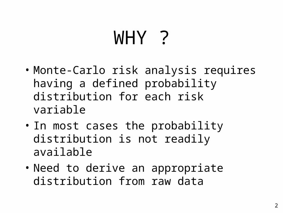
STEPS TO FOLLOW:1. Identify the risk variable and nature of risk

2. Obtain historical data on the variable

3. Transfer raw data into spreadsheet

4. Convert nominal values into real values

5. Calculate correlations among variables, if needed

6. Run a regression to identify a trend over years

7. Obtain residuals from regression

8. Express residuals as a percentage deviation from the trend

9. Rank the percentage deviations

10. Group percentage deviations into ranges

11. Specify frequency of occurrence for each range

12. Calculate the expected value

13. Make adjustments to frequencies, so that the expected value equals to the deterministic value of risk variable (check for the adjusted expected value)

14. Transfer the derived probability distribution into risk analysis software

4

1. IDENTIFY THE RISK VARIABLE AND NATURE OF RISK

• A financial/economic model of the project has to be complete

• Sensitivity analysis suggests candidates to be included as “risk

variables”

• A “risk variable” must be both risky (have a great impact on the

project) and uncertain (not predictable)

• Sensitivity analysis helps to identify the risky variables

• It is the task of analyst to understand the underlying reasons for

uncertainty of variable

5

QUESTIONS TO UNDERSTAND RISK

• What are the fundamental reasons for

movements of the variable over time?

• Can the causes of risk be predicted?

• Are there any related variables, which move in

the same or opposite direction at the same time?

• Is it possible to avoid the risk or reduce it

somehow?

6

2. OBTAIN HISTORICAL DATA ON THE VARIABLE

• Once the risk variable is identified and justified to be included into risk analysis

• Need to obtain a reliable set of data on the variable over time

• As many observations as possible

• If data on the variable itself is not available – use data on a related variable (fluctuations in the price of natural gas can be reasonably approximated by movements of the oil prices)

7

EXAMPLE: DERIVATION OF A PROBABILITY DISTRIBUTION FOR NATURAL GAS PRICE

• Natural gas is the major input for production of urea in a

fertilizer plant project

• Price of input was identified as a very risky variable, having a

strong impact on the project’s returns

• Project purchases natural gas as a price-taker

• Natural gas prices follow the international gas prices

• Prices can not be fully predicted – risk analysis is needed

8

• Data on the domestic and international gas prices were

not available

• It is believed that the crude oil prices can be used as a

proxy for fluctuations in the prices of natural gas

• Historic records of the crude oil prices supplied

by the OPEC were obtained from “OPEC Annual

Statistical Bulletin 2000” {www.opec.org}

• Crude oil prices are expressed in nominal US

dollar

9

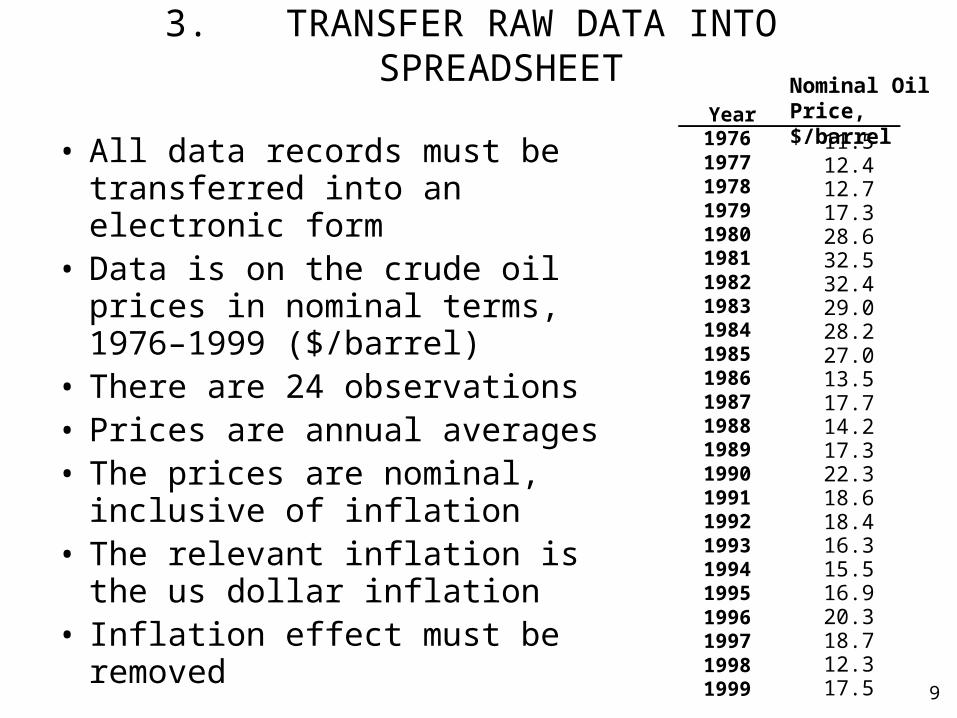
3. TRANSFER RAW DATA INTO SPREADSHEET

• All data records must be transferred into an electronic form

• Data is on the crude oil prices in nominal terms, 1976–1999 ($/barrel)

• There are 24 observations• Prices are annual averages• The prices are nominal, inclusive

of inflation• The relevant inflation is the us

dollar inflation• Inflation effect must be removed

Year

Nominal Oil Price, $/barrel

197619771978197919801981198219831984198519861987198819891990199119921993199419951996199719981999

11.512.412.717.328.632.532.429.028.227.013.517.714.217.322.318.618.416.315.516.920.318.712.317.5

10

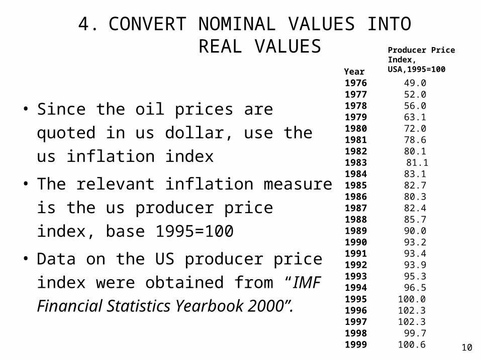
4. CONVERT NOMINAL VALUES INTO REAL VALUES

• Since the oil prices are quoted in us

dollar, use the us inflation index

• The relevant inflation measure is the us

producer price index, base 1995=100

• Data on the US producer price index

were obtained from “IMF Financial

Statistics Yearbook 2000”.

Year1976 49.01977 52.01978 56.01979 63.11980 72.01981 78.61982 80.11983 81.11984 83.11985 82.71986 80.31987 82.41988 85.71989 90.01990 93.21991 93.41992 93.91993 95.31994 96.51995 100.01996 102.31997 102.31998 99.71999 100.6

Producer Price Index, USA,1995=100

11

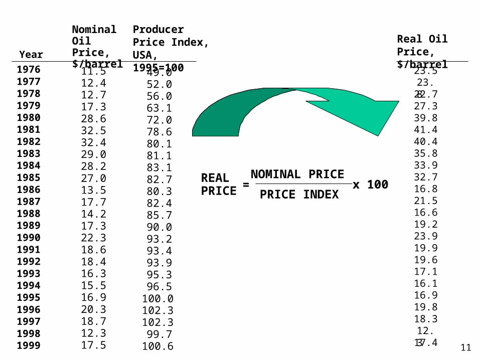
23.523.822.727.339.841.440.435.833.932.716.821.516.619.223.919.919.617.116.116.919.818.312.317.4

Real Oil Price, $/barrel

REAL PRICE

NOMINAL PRICE

PRICE INDEXx 100=

Year

Nominal Oil Price, $/barrel

197619771978197919801981198219831984198519861987198819891990199119921993199419951996199719981999

49.052.056.063.172.078.680.181.183.182.780.382.485.790.093.293.493.995.396.5

100.0102.3102.399.7

100.6

Producer Price Index, USA, 1995=100

11.512.412.717.328.632.532.429.028.227.013.517.714.217.322.318.618.416.315.516.920.318.712.317.5

12

5. CALCULATE CORRELATIONS BETWEEN VARIABLES

• If variables tend to move together over time – there is a

correlation

• Coefficient of correlation can be easily estimated from two

sets of data

• Both data sets must be expressed in real terms

• Example: correlation between the price of crude oil (input)

and price of urea fertilizer (output)

• Real price of urea was obtained from nominal price in the

same manner as real oil price

13

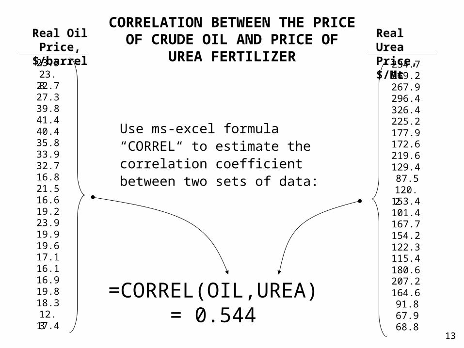
CORRELATION BETWEEN THE PRICE OF CRUDE OIL AND PRICE

OF UREA FERTILIZER

Use ms-excel formula “CORREL“ to estimate the correlation coefficient between two sets of data:

234.7269.2267.9296.4326.4225.2177.9172.6219.6129.487.5

120.2153.4101.4167.7154.2122.3115.4180.6207.2164.691.867.968.8

Real Urea Price, $/Mt

=CORREL(OIL,UREA)= 0.544

23.523.822.727.339.841.440.435.833.932.716.821.516.619.223.919.919.617.116.116.919.818.312.317.4

Real Oil Price, $/barrel

14

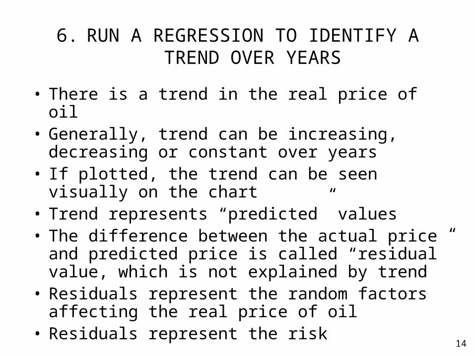
6. RUN A REGRESSION TO IDENTIFY A TREND OVER YEARS

• There is a trend in the real price of oil• Generally, trend can be increasing, decreasing or

constant over years• If plotted, the trend can be seen visually on the chart• Trend represents “predicted” values• The difference between the actual price and predicted

price is called “residual” value, which is not explained by trend

• Residuals represent the random factors affecting the real price of oil

• Residuals represent the risk

15

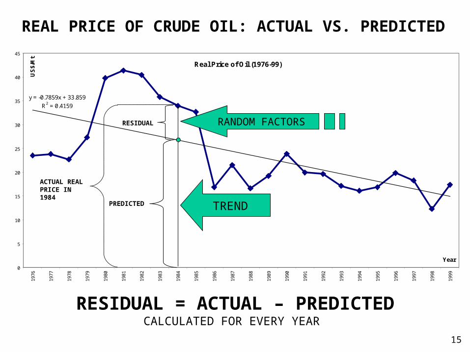
Real Price of Oil (1976-99)

y = -0.7859x + 33.859

R2 = 0.4159

0

5

10

15

20

25

30

35

40

45

1976

1977

1978

1979

1980

1981

1982

1983

1984

1985

1986

1987

1988

1989

1990

1991

1992

1993

1994

1995

1996

1997

1998

1999

Year

US

$/M

tREAL PRICE OF CRUDE OIL: ACTUAL VS. PREDICTED

PREDICTED

RESIDUAL

ACTUAL REAL PRICE IN 1984

TREND

RANDOM FACTORS

RESIDUAL = ACTUAL – PREDICTEDCALCULATED FOR EVERY YEAR

16

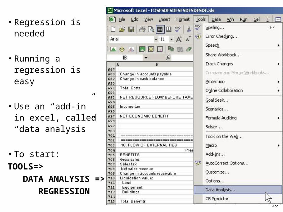
• Regression is needed

• Running a regression is easy

• Use an “add-in” in excel, called “data analysis”

• To start:

TOOLS=>

DATA ANALYSIS =>

REGRESSION

17

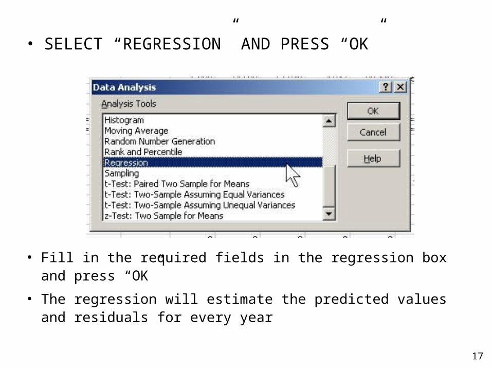
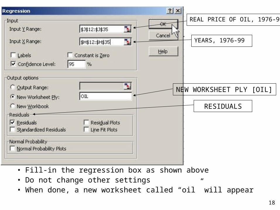
• Fill in the required fields in the regression box and press “OK”

• The regression will estimate the predicted values and residuals for every year

• SELECT “REGRESSION” AND PRESS “OK”

18

YEARS, 1976-99

NEW WORKSHEET PLY [OIL]

RESIDUALS

• Fill-in the regression box as shown above• Do not change other settings• When done, a new worksheet called “oil” will appear

REAL PRICE OF OIL, 1976-99

19

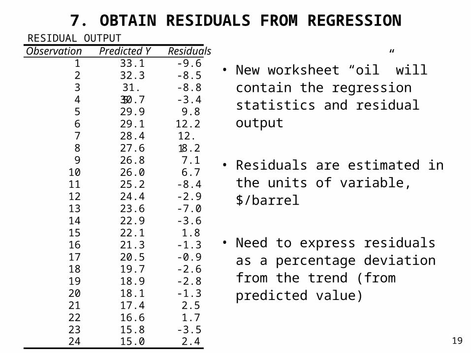
• New worksheet “oil” will contain the regression statistics and residual output

• Residuals are estimated in the units of variable, $/barrel

• Need to express residuals as a percentage deviation from the trend (from predicted value)

RESIDUAL OUTPUTObservation Predicted Y Residuals

1 33.1 -9.62 32.3 -8.53 31.5 -8.84 30.7 -3.45 29.9 9.86 29.1 12.27 28.4 12.18 27.6 8.29 26.8 7.1

10 26.0 6.711 25.2 -8.412 24.4 -2.913 23.6 -7.014 22.9 -3.615 22.1 1.816 21.3 -1.317 20.5 -0.918 19.7 -2.619 18.9 -2.820 18.1 -1.321 17.4 2.522 16.6 1.723 15.8 -3.524 15.0 2.4

7. OBTAIN RESIDUALS FROM REGRESSION

20

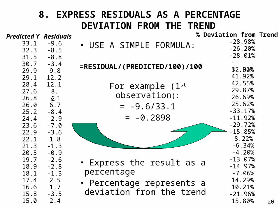
8. EXPRESS RESIDUALS AS A PERCENTAGE DEVIATION FROM THE TREND

• USE A SIMPLE FORMULA:

=RESIDUAL/(PREDICTED/100)/100

For example (1st observation):

= -9.6/33.1= -0.2898

• Express the result as a percentage• Percentage represents a deviation from the trend

Predicted Y Residuals33.1 -9.632.3 -8.531.5 -8.830.7 -3.429.9 9.829.1 12.228.4 12.127.6 8.226.8 7.126.0 6.725.2 -8.424.4 -2.923.6 -7.022.9 -3.622.1 1.821.3 -1.320.5 -0.919.7 -2.618.9 -2.818.1 -1.317.4 2.516.6 1.715.8 -3.515.0 2.4

% Deviation from Trend-28.98%-26.20%-28.01%-11.00%32.91%41.92%42.55%29.87%26.69%25.62%-33.17%-11.92%-29.72%-15.85%

8.22%-6.34%-4.20%

-13.07%-14.97%-7.06%14.29%10.21%-21.96%15.80%

21

9. RANK THE PERCENTAGE DEVIATIONS

• Residuals in percentage form represent the

deviations from the trend

• The percentage deviations must be ranked from

the lowest to highest

• Use a built-in “sort” function in excel:

1. Highlight all percentage deviations

2. Open “DATA” => “SORT…”

3. Fill-in the sorting box

22

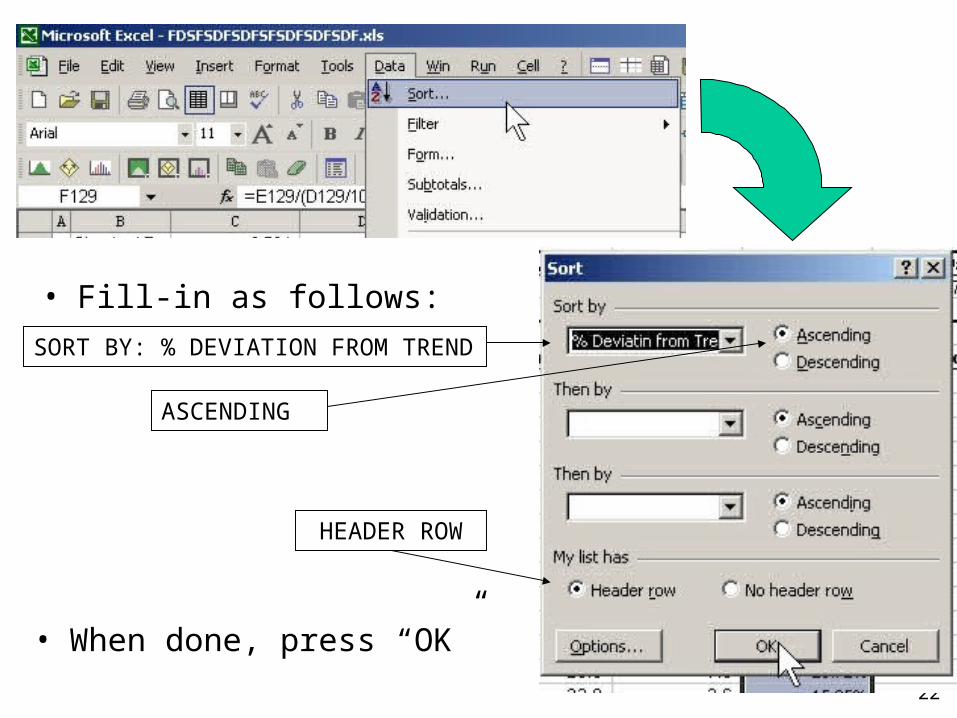
• Fill-in as follows:

SORT BY: % DEVIATION FROM TREND

ASCENDING

HEADER ROW

• When done, press “OK”

23

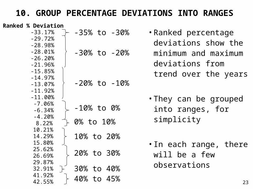
• Ranked percentage deviations show the minimum and maximum deviations from trend over the years

• They can be grouped into ranges, for simplicity

• In each range, there will be a few observations

10. GROUP PERCENTAGE DEVIATIONS INTO RANGES

Ranked % Deviation-33.17%-29.72%-28.98%-28.01%-26.20%-21.96%-15.85%-14.97%-13.07%-11.92%-11.00%-7.06%-6.34%-4.20%8.22%

10.21%14.29%15.80%25.62%26.69%29.87%32.91%41.92%42.55%

-35% to -30%

-30% to -20%

-20% to -10%

-10% to 0%

0% to 10%

10% to 20%

20% to 30%

30% to 40%40% to 45%

24

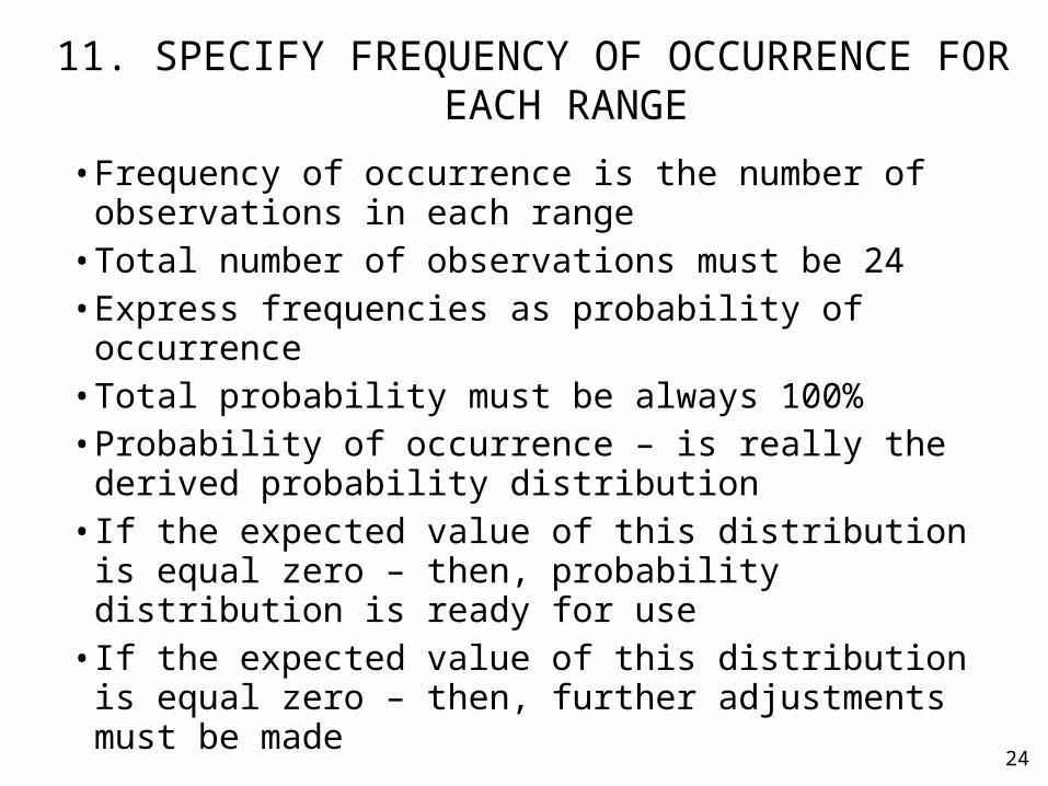
11. SPECIFY FREQUENCY OF OCCURRENCE FOR EACH RANGE

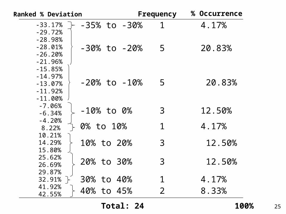
• Frequency of occurrence is the number of observations in each range

• Total number of observations must be 24• Express frequencies as probability of occurrence• Total probability must be always 100%• Probability of occurrence – is really the derived

probability distribution• If the expected value of this distribution is equal zero –

then, probability distribution is ready for use• If the expected value of this distribution is equal zero –

then, further adjustments must be made

25

Ranked % Deviation

-33.17%-29.72%-28.98%-28.01%-26.20%-21.96%-15.85%-14.97%-13.07%-11.92%-11.00%-7.06%-6.34%-4.20%8.22%

10.21%14.29%15.80%25.62%26.69%29.87%32.91%41.92%42.55%

-35% to -30% 1 4.17%

-30% to -20% 5 20.83%

-20% to -10% 5 20.83%

-10% to 0% 3 12.50%

0% to 10% 1 4.17%

10% to 20% 3 12.50%

20% to 30% 3 12.50%

30% to 40% 1 4.17%40% to 45% 2 8.33%

Frequency % Occurrence

Total: 24 100%

26

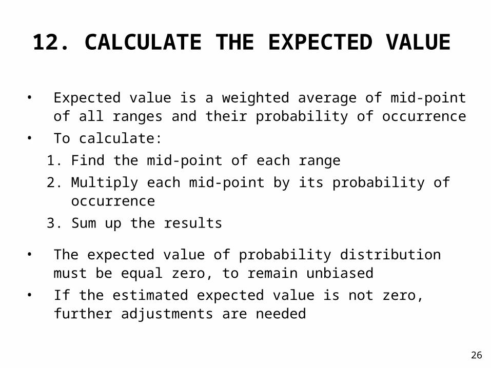
• Expected value is a weighted average of mid-point of all ranges and their probability of occurrence

• To calculate:

1. Find the mid-point of each range

2. Multiply each mid-point by its probability of occurrence

3. Sum up the results

• The expected value of probability distribution must be equal zero, to remain unbiased

• If the estimated expected value is not zero, further adjustments are needed

12. CALCULATE THE EXPECTED VALUE

27

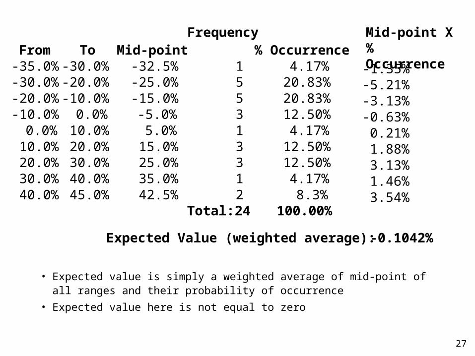
• Expected value is simply a weighted average of mid-point of all ranges and their probability of occurrence

• Expected value here is not equal to zero

From To Mid-pointFrequency

% OccurrenceMid-point X % Occurrence

-35.0% -30.0% -32.5% 1 4.17% -1.35%-30.0% -20.0% -25.0% 5 20.83% -5.21%-20.0% -10.0% -15.0% 5 20.83% -3.13%-10.0% 0.0% -5.0% 3 12.50% -0.63%

0.0% 10.0% 5.0% 1 4.17% 0.21%10.0% 20.0% 15.0% 3 12.50% 1.88%20.0% 30.0% 25.0% 3 12.50% 3.13%30.0% 40.0% 35.0% 1 4.17% 1.46%40.0% 45.0% 42.5% 2 8.3% 3.54%

Total: 24 100.00%

Expected Value (weighted average): -0.1042%

28

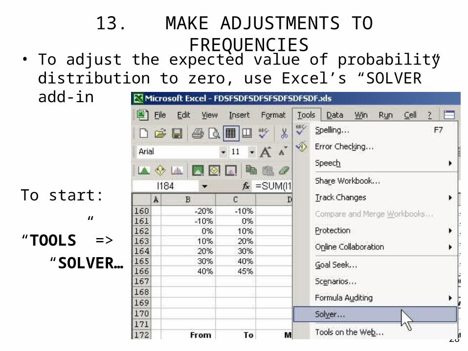
13. MAKE ADJUSTMENTS TO FREQUENCIES• To adjust the expected value of probability distribution to zero,

use Excel’s “SOLVER” add-in

To start:

“TOOLS” =>

“SOLVER…”

29

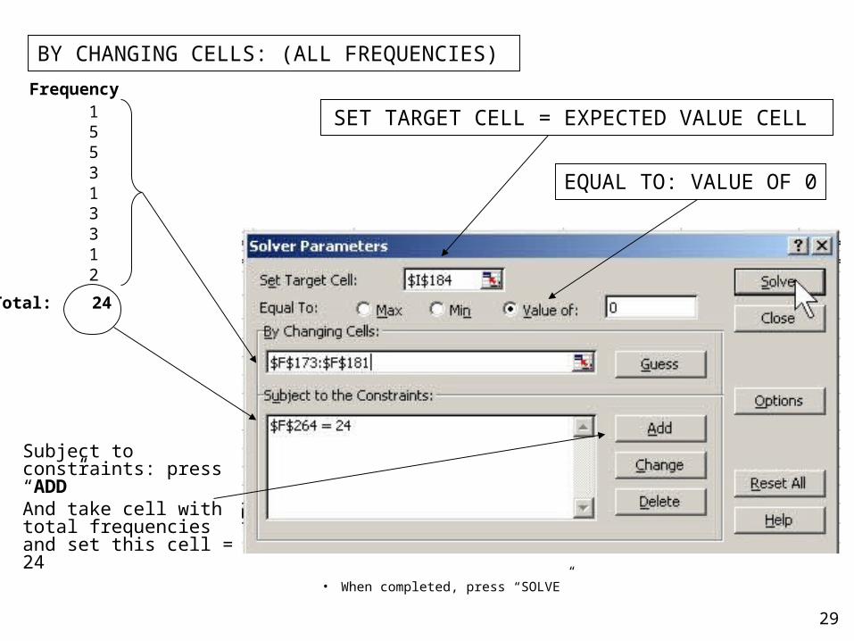
Subject to constraints: press “ADD” And take cell with total frequencies and set this cell = 24

SET TARGET CELL = EXPECTED VALUE CELL

EQUAL TO: VALUE OF 0

BY CHANGING CELLS: (ALL FREQUENCIES)

Frequency155313312

Total: 24

• When completed, press “SOLVE”

30

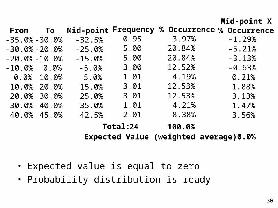
• Expected value is equal to zero

• Probability distribution is ready

Total:

Frequency % OccurrenceMid-point X % Occurrence

0.95 3.97% -1.29%5.00 20.84% -5.21%5.00 20.84% -3.13%3.00 12.52% -0.63%1.01 4.19% 0.21%3.01 12.53% 1.88%3.01 12.53% 3.13%1.01 4.21% 1.47%2.01 8.38% 3.56%

24 100.0%Expected Value (weighted average): 0.0%

From To Mid-point-35.0% -30.0% -32.5%-30.0% -20.0% -25.0%-20.0% -10.0% -15.0%-10.0% 0.0% -5.0%

0.0% 10.0% 5.0%10.0% 20.0% 15.0%20.0% 30.0% 25.0%30.0% 40.0% 35.0%40.0% 45.0% 42.5%

31

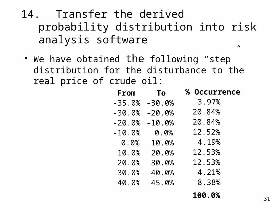
14. Transfer the derived probability distribution into risk analysis software

• We have obtained the following “step” distribution for the disturbance to the real price of crude oil:

% Occurrence3.97%

20.84%20.84%12.52%

4.19%12.53%12.53%

4.21%8.38%

100.0%

From To-35.0% -30.0%-30.0% -20.0%-20.0% -10.0%-10.0% 0.0%

0.0% 10.0%10.0% 20.0%20.0% 30.0%30.0% 40.0%40.0% 45.0%

32

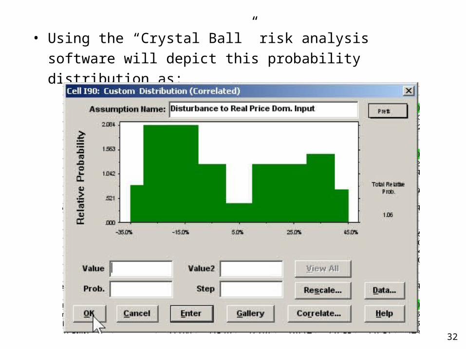
• Using the “Crystal Ball” risk analysis software will depict this

probability distribution as:

33

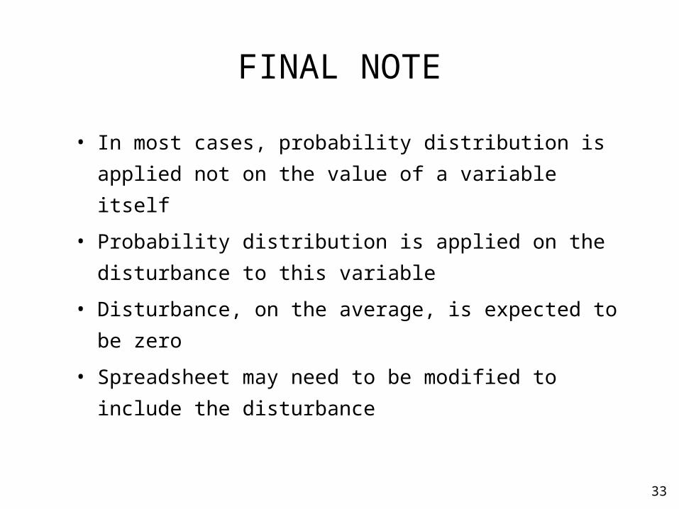
FINAL NOTE

• In most cases, probability distribution is applied not on the

value of a variable itself

• Probability distribution is applied on the disturbance to this

variable

• Disturbance, on the average, is expected to be zero

• Spreadsheet may need to be modified to include the

disturbance

34

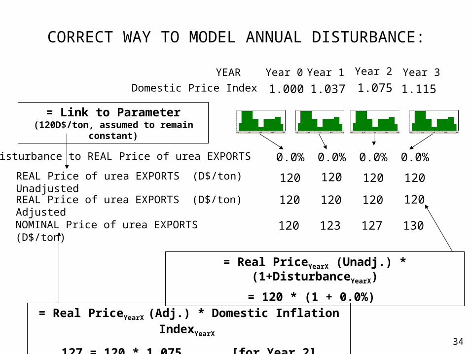
CORRECT WAY TO MODEL ANNUAL DISTURBANCE:

Disturbance to REAL Price of urea EXPORTS 0.0% 0.0% 0.0% 0.0%

REAL Price of urea EXPORTS (D$/ton) Adjusted 120 120 120 120

NOMINAL Price of urea EXPORTS (D$/ton) 120 123 127 130

= Real PriceYearX (Unadj.) * (1+DisturbanceYearX)

= 120 * (1 + 0.0%)

= Real PriceYearX (Adj.) * Domestic Inflation IndexYearX

127 = 120 * 1.075 [for Year 2]

YEAR Year 0 Year 1 Year 2 Year 3

Domestic Price Index 1.000 1.037 1.075 1.115

REAL Price of urea EXPORTS (D$/ton) Unadjusted 120 120 120 120

= Link to Parameter (120D$/ton, assumed to remain constant)