5946 IEEE TRANSACTIONS ON INFORMATION …elib.dlr.de/72163/1/10.1.1.220.6721(1).pdf5946 IEEE TRANSACTIONS ON INFORMATION THEORY, VOL. 57, NO. 9, SEPTEMBER 2011 An Interpolation Procedure

5946 IEEE TRANSACTIONS ON INFORMATION THEORY, VOL. 57, NO. 9, SEPTEMBER 2011

An Interpolation Procedure for List DecodingReed–Solomon Codes Based on

Generalized Key EquationsAlexander Zeh, Student Member, IEEE, Christian Gentner, Member, IEEE, and Daniel Augot

Abstract—The key step of syndrome-based decoding ofReed–Solomon codes up to half the minimum distance is tosolve the so-called Key Equation. List decoding algorithms, ca-pable of decoding beyond half the minimum distance, are basedon interpolation and factorization of multivariate polynomials.This article provides a link between syndrome-based decoding ap-proaches based on Key Equations and the interpolation-based listdecoding algorithms of Guruswami and Sudan for Reed–Solomoncodes. The original interpolation conditions of Guruswami andSudan for Reed–Solomon codes are reformulated in terms ofa set of Key Equations. These equations provide a structuredhomogeneous linear system of equations of Block-Hankel form,that can be solved by an adaption of the Fundamental IterativeAlgorithm. For an �� Reed–Solomon code, a multiplicity � anda list size �, our algorithm has time complexity ��.

Index Terms—Block-Hankel matrix, fundamental iterative algo-rithm (FIA), Guruswami–Sudan interpolation, key equation, listdecoding, Reed–Solomon codes.

I. INTRODUCTION

I N 1999, Guruswami and Sudan [3]–[5] extended Sudan’soriginal approach [6] by introducing multiplicities in the

interpolation step of their polynomial-time list decoding proce-dure for Reed–Solomon and Algebraic Geometric codes. Thismodification permits decoding of Reed–Solomon codes[7] (and Algebraic Geometric codes) of arbitrary code-rate

with increased decoding radius. Guruswami andSudan were focused on the existence of a polynomial-timealgorithm. Kötter [8] and Roth-Ruckenstein [9], [10] pro-posed quadratic time algorithms for the key steps of theGuruswami–Sudan principle for Reed–Solomon codes, i.e.,

Manuscript received September 03, 2009; revised September 13, 2010; ac-cepted April 10, 2011. Date of current version August 31, 2011. This workwas supported by the German Research Council “Deutsche Forschungsgemein-schaft” (DFG) by Grant No. Bo867/22-1. The material in this paper was pre-sented at the IEEE International Symposium on Information Theory, Toronto,ON, Canada, 2008, and at the IEEE Information Theory Workshop, Taormina,Sicily, Italy, 2009.

A. Zeh is with the Institute of Telecommunications and Applied In-formation Theory, University of Ulm, Germany, and also with theINRIA—Saclay-Île-de-France and École Polytechnique, Paris, France(e-mail: [email protected]).

C. Gentner is with the Institute of Communications and Navigation of theGerman Aerospace Center (DLR), Germany (e-mail: [email protected]).

D. Augot is with INRIA—Saclay-Île-de-France and École Polytechnique,Paris, France (e-mail: [email protected]).

Communicated by M. Blaum, Associate Editor for Coding Theory.Digital Object Identifier 10.1109/TIT.2011.2162160

interpolation and factorization of bivariate polynomials. Var-ious other approaches for a low-complexity realization ofGuruswami–Sudan exist, e.g., the work of Alekhnovich [11],where fast computer algebra techniques are used. Trifonov’s[12] contributions rely on ideal theory and divide and conquermethods. Sakata uses Gröbner-bases techniques [13], [14].

In this paper, we reformulate the bivariate interpolation stepof Guruswami–Sudan for Reed–Solomon codes in a set of uni-variate Key Equations [1]. This extends the previous work ofRoth and Ruckenstein [9], [10], where the reformulation wasdone for the special case of Sudan. Furthermore, we present amodification of the so-called Fundamental Iterative Algorithm(FIA), proposed by Feng and Tzeng in 1991 [15]. Adjusted tothe special case of one Hankel matrix the FIA resembles the ap-proach of Berlekamp and Massey [16], [17].

Independently of our contribution, Beelen and Høholdt refor-mulated the Guruswami–Sudan constraints for Algebraic Geo-metric codes [18], [19]. It is not clear, if the system they obtainis highly structured.

This contribution is organized as follows. The next sectioncontains basic definitions for Reed–Solomon codes and bi-variate polynomials. In Section III, we derive the Key Equationfor conventional decoding of Reed–Solomon codes from theWelch-Berlekamp approach [20] and we present the adjust-ment of the FIA for one Hankel matrix. A modified versionof Sudan’s reformulated interpolation problem based on thework of Roth-Ruckenstein [9] is derived and the adjustment ofthe FIA for this case is illustrated in Section IV. In Section V,the interpolation step of the Guruswami–Sudan principle isreformulated. The obtained homogeneous set of linear equa-tions has Block-Hankel structure. We adjust the FIA for thisBlock-Hankel structure, prove the correctness of the proposedalgorithm and analyze its complexity. We conclude this contri-bution in Section VI.

II. DEFINITIONS AND PRELIMINARIES

Throughout this paper, denotes the set of inte-gers and denotes the set of integers

. An matrix consistsof the entries , where and . A uni-variate polynomial of degree less than is denoted by

. A vector of length is represented by.

Let be a power of a prime and let denote thefinite field of order . Let denote nonzero dis-tinct elements (code-locators) of and let denote

0018-9448/$26.00 © 2011 IEEE

ZEH et al.: INTERPOLATION PROCEDURE FOR LIST DECODING REED–SOLOMON CODES 5947

nonzero elements (column-multipliers), the associated evalua-tion map ev is

(1)

The associated Generalized Reed–Solomon code oflength and dimension is [21]

(2)

where denotes the set of all univariate polynomials withdegree less than . Generalized Reed–Solomon codes are MDScodes with minimum distance . The dual of a Gen-eralized Reed–Solomon is also a Generalized Reed–Solomoncode with the same code locators and column multipliers

, where . Theexplicit form of the column multipliers is [22]

(3)

We will take advantage of structured matrices and thereforewe recall the definition of a Hankel matrix in the following.

Definition 1 (Hankel Matrix): An Hankel matrixis a matrix, where for all

and holds.Let us recall some properties of bivariate polynomials in

.

Definition 2 (Weighted Degree): Let the polynomialbe in . Then, the

-weighted degree of , denoted by ,

is the maximum over all such that .

Definition 3 (Multiplicity and Hasse Derivative [23]): Letbe a polynomial in . Let

. A bivariatepolynomial has at least multiplicity in the point

, denoted by

(4)

if the coefficients are zero for all . Furthermore,the th Hasse derivative of the polynomial in thepoint is

(5)

Let denote the th Hasse derivative ofwith respect to the variable .

We will use the inner product for bivariate polynomials todescribe our algorithms.

Definition 4 (Inner Product): Let two polynomialsand

in be given. The inner product ofand is defined by .

III. WELCH-BERLEKAMP AS LIST-ONE DECODER AND THE

FUNDAMENTAL ITERATIVE ALGORITHM

A. Syndrome-Based Decoding of Reed–Solomon Codes

Let denote the error word and letbe the set of error locations (that is ). Let

. It is well known that a code canrecover uniquely any error pattern if and only if . The

syndrome coefficients depend onlyon the error word and the associated syndrome polynomial

is defined by [22]

The error-locator polynomial is and theerror-evaluator polynomial is

. They are related by the Key Equation:

(6)

The main steps for conventional decoding up to half the min-imum distance are:

1) Calculate the syndrome polynomial from the re-ceived word .

2) Solve (6) for the error-locator polynomial and deter-mine its roots.

3) Compute and then determine the error values.

B. Derivation of the Key Equation From Welch-Berlekamp

We derive the classical Key Equation (6) from the simplest in-terpolation based decoding algorithm, reported as the “Welch-Berlekamp” decoding algorithm in [24]–[26]. We provide a sim-pler representation than in [20] and give a polynomial derivationof the Key Equation.

Consider a code with support set ,multipliers and dimension . The Welch-Berlekamp approach is based on the following lemma [27, Ch.5.2].

Lemma 1 (List-One Decoder): Let be a code-word of a code and letbe the received word. We search for a polynomial

in such that:1) ,2) ,3) .

If has distance less than or equal to from thereceived word , then .

Let us connect Lemma 1 to (6).

Proposition 1 (Univariate Reformulation): Letbe the Lagrange interpolation polynomial, such that

holds. Let .Then satisfies Conditions 2)


and 3) of Lemma 1 if and only if there exists a polynomialsuch that

(7)

and .Let . Define the followingreciprocal polynomials:

(8)

Inverting the order of the coefficients of (7) leads to:

With (8), we obtain:

which we can consider modulo . We obtain

(9)

Since , we can define the formal power series:

(10)

Using the column multipliers (3) for the dual code, it can beverified that is the series of syndromes with

(11)

Thus, dividing (9) by , we obtain

(12)

which corresponds to the classical Key Equation (6). The syn-drome polynomial is , and is the error-locator polynomial .

In the case of errors, we consider only the terms of theKey Equation of degree greater than and we get thefollowing homogeneous linear system of equations:

......

......

(13)

The above syndrome matrix for all andhas Hankel form (see Definition 1). Equation (12)

can be solved by the well-known Berlekamp-Massey algorithm[16], [17] or with a modification of the Extended Euclidean al-gorithm [28]. The parallels of the Berlekamp-Massey algorithmand the Extended Euclidean algorithm have been considered in[29]–[31].

We consider in the following the FIA [15], that can be usedto find the first linearly dependent columns and connec-tion coefficients for an arbitrary matrix. The FIAallows a significant reduction of complexity when adjusted to aHankel matrix as in (13).

C. The FIA for One Hankel Matrix

Given an arbitrary matrix , the FIAoutputs the minimal number of linearly dependentcolumns together with the polynomial ,with , such that holds.The FIA scans the th column of the matrix row-wise in theorder and uses previously stored polynomials toupdate the current polynomial . Let be the index of thecurrent column under inspection, and letbe the current candidate polynomial that satisfies

for some value of the row index . In other words, the coeffi-cients of the polynomial give us the vanishing linear com-bination of the matrix consisting of the first rows and the first

columns of the matrix . Suppose that the discrepancy

(14)

for next row is nonzero. If there exists a previously storedpolynomial and a nonzero discrepancy , corre-sponding to row , then the current polynomial is updatedin the following way:

(15)

The proof of the above update rule is straightforward [15].In the case and there is no discrepancy stored,

the actual discrepancy is stored as . The correspondingauxiliary polynomial is stored as . Then, the FIA exam-ines a new column .

Definition 5 (True Discrepancy): Let the FIA examine theth row of the th column of matrix . Furthermore, let the

calculated discrepancy (14) be nonzero and no other nonzerodiscrepancy be stored for row . Then, the FIA examines a newcolumn . We call this case a true discrepancy.

Theorem 1 (Correctness and Complexity of the FIA [15]):For an matrix with , the Fundamental IterativeAlgorithm stops, when the row pointer has reached the last row


Fig. 1. Illustration of the row pointer � of the classic FIA [(a)] and of the adjusted FIA [b)] when both algorithms are applied to the same 6� 7 Hankel syndromematrix of a �� code. The dots indicate a true discrepancy. In this case, both algorithms enter a new column, but with different initial values of their rowpointers.

of column . Then, the last polynomial corresponds toa valid combination of the first columns. The complexityof the algorithm is .

For a Hankel matrix (as in Definition 1), the FIA can beadjusted. Assume the case of a true discrepancy, when the FIAexamines the th row of the th column of the structured matrix

. The current polynomial is . Then, the FIA starts exam-ining the th column at row withand not at row zero. This reduces the cubic time complexity intoa quadratic time complexity [15].

To illustrate the complexity reduction of the FIA when ad-justed to a Hankel matrix (compared to the original, unadjustedFIA), we traced the examined rows for each column in Fig. 1.Fig. 1(a) shows the values of of the FIA without any adaption.The row pointer of the adapted FIA is traced in Fig. 1(b).

The points on the lines in both figures indicate the case, wherea true discrepancy has been encountered.

IV. SUDAN INTERPOLATION STEP WITH A HORIZONTAL BAND

OF HANKEL MATRICES

A. Univariate Reformulation of the Sudan Interpolation Step

In this section, we recall parts of the work of Roth and Ruck-enstein [9], [10] for the interpolation step of the Sudan [6] prin-ciple. The aimed decoding radius is denoted by , the corre-sponding list size is .

Problem 1 (Sudan Interpolation Step [6]): Let the aimeddecoding radius and the received word begiven. The Sudan interpolation step determines a polynomial

, such that1) ;,2) ;3) .

We present here a slightly modified version of [9], to get anappropriate basis for the extension to the interpolation step inthe Guruswami–Sudan case.

We have. Let be the Lagrange interpolation polynomial,

s.t. and .The reciprocal polynomial of is denoted by

.Similar to Proposition 1, Roth-Ruckenstein [9] proved the

following. There is an interpolation polynomial satis-fying Conditions (2) and (3) if and only if there exists a uni-variate polynomial with degree smaller than ,s.t. .

Let the reciprocal polynomials be defined as in (8). From [9,(19)] we have

(16)

where . We introduce the power series

(17)

Inserting (17) into (16) leads to

(18)

Based on (18) we can now define syndromes for Problem 1.

Definition 6 (Syndromes for Sudan): The generalizedsyndrome polynomials are givenby

(19)

The first-order Extended Key Equation is

(20)


with .An explicit form of is

(21)

Note 1: In [9], a further degree reduction is proposed. Then(18), is modulo and the polynomial disappears.We do not present this improvement here, because we cannotproperly reproduce this behavior in the Guruswami–Sudan case(see Note 2).The degree of the LHS of (16) is smaller than .If we consider the terms of degree higher than , weobtain homogeneous linear equations. Reverting back to theoriginals univariate polynomials , we get the followingsystem:

(22)

With , we obtain the fol-lowing matrix form:

...(23)

where each submatrixis a Hankel matrix. The syndrome polynomials

of Definition 6 are associated withthis horizontal band of Hankel matrices by .

In the following, we describe how the FIA can be adapted tosolve the homogeneous system of (23).

B. Adjustment of the FIA for the Reformulated SudanInterpolation Problem

The FIA can directly be applied to the matrixof (23), but if we want to take ad-

vantage of the Hankel structure we have to scan the columns ofin a manner given by the weighted degree

requirement of the interpolation problem.

Let denote the ordering for the pairs, where is given by

(24)

The pair that immediately follows with respect tothe order defined by is denoted by . Thecolumns of the matrix are reorderedaccording to . The pair indexes the th column of

th submatrix . More explicitly, we obtain the followingmatrix , where the columns of are reordered [see (25) atthe bottom of the page].

The corresponding homogeneous system of equations cannow be written in terms of the inner product for bivariate poly-nomials (see Definition 4).

Problem 2 (Reformulated Sudan Interpolation Problem): Letthe syndrome polynomials

be given by Definition 6 and let bethe corresponding bivariate syndrome polynomial. We search anonzero bivariate polynomial such that

(26)

Hence, the bivariate polynomial is a valid interpo-lation polynomial for Problem 1. Note that each polynomial

, as defined in (16), has degree smaller than .To index the columns of the rearranged matrix , let

(27)

Algorithm 1 is the modified FIA for solving Problem 2. In con-trast to the original Roth-Ruckenstein adaption we consider allhomogeneous linear equations (instead of ), according to Note1. The column pointer is given by , for indexing the thcolumn of the th submatrix . Algorithm 1 virtually scansthe rearranged matrix column after column (see Line 23 ofAlgorithm 1). The true discrepancy value for row is stored inarray as , and the corresponding intermediate bivariatepolynomial is stored in array as . The discrepancy calcu-lation and the update rule [see (14) and (15) for the basic FIA] isadapted to the bivariate case (see Line 16 of Algorithm 1). Foreach submatrix , the previous value of the row pointer is

......

......

......

......

...

(25)


stored in an array as . We prove the initialization rule forthe FIA solving Problem 2 in the following proposition.

Proposition 2 (Initialization Rule): Assume Algo-rithm 1 examines column of a syndrome matrix

as defined in (23) (or equiva-lently the bivariate polynomial ). Assume that a truediscrepancy is obtained in row .

Let . Hence, Algorithm 1 canexamine column at row with the initial value

, where is the index of the row,where the last true discrepancy in the th submatrix wascalculated. The polynomial is the stored intermediatepolynomial for , i.e., and .

Proof: In terms of the inner product (see Definition 4), wehave

Let us write . We have

and we compute

which is zero for the rows of index .

Similarly to the FIA for one Hankel matrix we can start ex-amining a new th column of the submatrix in row .Note that the previous value of the row pointer is stored in

.Before Algorithm 1 enters a new column, the coefficients of

the intermediate bivariate connection polynomial giveus the vanishing linear combination of the submatrix consistingof the first rows and previous columns of the rearrangedmatrix (see (25)). The following theorem summarizes theproperties of Algorithm 1.

Theorem 2 (Algorithm 1): Let bethe matrix as defined in (23) and the as-sociated bivariate syndrome polynomial for the reformulatedSudan interpolation problem. Algorithm 1 returns a bivariatepolynomial such that:

The time complexity of Algorithm 1 is .Proof: The correctness of Algorithm 1 follows from the

correctness of the basic FIA (see Theorem 1) and from the cor-rectness of the initialization rule (Proposition 2) considering thatAlgorithm 1 deals with the column-permuted version of theoriginal matrix .

The proof of the complexity of Algorithm 1 is as follows. Wetrace the triple

where is the current column pointer of Algorithm 1 ex-amining the th column of the th submatrix . The vari-ables , are the values of the last row reached in thesubmatrices . These values are stored in thearray in Algorithm 1. The value is the number of alreadyencountered true discrepancies of Algorithm 1. Assumeis the current column pointer of Algorithm 1. The two followingevents in Algorithm 1 can happen.


Fig. 2. Illustration of the row pointer � of Algorithm 1 applied to a horizontal band of three Hankel matrices � � � and � . The columns of the 16� 18matrix � are arranged under � -ordering. The three lines � � � and � trace the row pointer for each submatrix � � � and � .

1) Either, there is no true discrepancy, then Algorithm 1 staysin the same column and increases by one. The triple becomes

2) Or, there is a true discrepancy, then Algorithm 1 examinescolumn and the triple becomes

For both cases, the sum over the triple is

(28)

when Algorithm 1 examines the th column of the ma-trix . From (27), we have

. The sum increases by one in each iteration ofAlgorithm 1. The initial value of is zero and the last valuecan be bounded by

Each discrepancy computation costs and Algorithm 1does not have to examine more than the th columns ofthe matrix . Thus, the totalcost of Algorithm 1 is .

In the following, we illustrate the values of the row pointerof Algorithm 1, when applied to a syndrome matrix

that consists of three Hankel matrices.

C. Example: Sudan Decoding of a Generalized Reed–SolomonCode With Adapted FIA

We consider a code over . For a decodingradius , the list size is . Thedegrees of the three univariate polynomialsand are limited to and we

TABLE ICOLUMN-INDEX � AND COLUMN POINTER �� OF THE RE-ARRANGED

MATRIX � OF THE REFORMULATED SUDAN INTERPOLATION STEP FOR A

�� CODE WITH DECODING RADIUS � � � AND LIST SIZE � � �

have more unknowns than interpolation constraints.

Fig. 2 illustrates the row pointer of Algorithm 1 when the16 18 syndrome matrix is examined. Thecolumns of the syndrome matrix are virtually rearrangedaccording to the -ordering and Algorithm 1 scans therearranged matrix column by column. The column-index

[see (27)] and the corresponding column pointerare listed in Table I.

The three zig-zag lines , and in Fig. 2 tracethe value of the row pointer for the three submatrices

and , which have a Hankel structure. The dots indicatethe case, where a true discrepancy occurs. After the th column(here ), every second column corresponds to the samesubmatrix.

After column 10 of the rearranged matrix , every thirdcolumn of corresponds to the same submatrix . Let usinvestigate two cases, where a true discrepancy in Algorithm 1occurs. They are marked in column andof the rearranged in Fig. 2. In between column 12 and 15one column of the submatrices and is examined byAlgorithm 1. In column (0, 8), Algorithm 1 starts investigating


the second row, because the true discrepancy in column (0, 7)occurred in the third row (according to Proposition 2).

D. The FIA for a Vertical Band of Hankel Matrices

The FIA can also be adapted to find the first linearlydependent columns of a matrix consisting of Hankel matricesarranged vertically. This case has been considered, for examplein [2] and [32]. The basic idea for such a vertical band of Hankelmatrices is the same as in the previous case. The rows of eachsubmatrix of Hankel structure are scanned in a similar inter-leaving order as the columns of the previous case.

The obtained time complexity for a vertical band of Hankelmatrices, where each submatrix consist of columns, is

.

V. GURUSWAMI–SUDAN INTERPOLATION STEP WITH A

BLOCK-HANKEL MATRIX

A. The Guruswami–Sudan Interpolation Step for GeneralizedReed–Solomon Codes

We consider again a Generalized Reed–Solomon code withsupport set , multipliers anddimension , as introduced in Section II. Letaccording to (3) be the multipliers of the dual GeneralizedReed–Solomon code.

Let be the received word. The Gu-ruswami–Sudan decoding principle [3]–[5] improves theprevious algorithms by introducing an additional param-eter , which is the order of multiplicity for the points

. The parameterinfluences the decoding radius and the list size . The rela-tionship between these parameters has been discussed in manypublications (see, e.g., [33]).

Problem 3 (Guruswami–Sudan Interpolation Step [3]):Let the aimed decoding radius , the multiplicity andthe received word be given. The Gu-ruswami–Sudan interpolation step determines a polynomial

, such that1) ,2) ,3) .

As in the previous section, let denote the degree of theunivariate polynomials . From Condition 3) of Problem3 we get

(29)

B. Univariate Reformulation of the Guruswami–SudanInterpolation Problem and a Block-Hankel Matrix

We reformulate the Guruswami–Sudan interpolation problemto obtain not one, but a system of several Extended Key Equa-tions. The corresponding homogeneous linear system has aBlock-Hankel form.

Proposition 3 (Univariate Reformulation): Let the integersand the received vector be given. Let

be the Lagrange interpolation polynomial, such that

. Let . A polynomialsatisfies Conditions 2) and 3) of Problem 3, if and only

if there exist polynomials such that

(30)

and .Note that denotes the th Hasse derivative of the bi-variate polynomial with respect to the variable (seeDefinition 3).

We first prove the following lemma.

Lemma 2: Let be given, and letbe any polynomial such that . A polynomial

has multiplicity at least at if and only if.

Proof: After translation to the origin, we can assume that, and , i.e., . Let

, where is homogeneous of degree .We first suppose that has at least a multiplicity at

(0, 0), i.e., , for . Hence, we have

For , the polynomials have no terms of degreeless than , and with , we have .It follows, that divides for all .

Suppose for the converse that . That is,, for some polynomials

and . Using Taylor’s formula with the Hasse derivatives[22, p. 89] we have

Now, has only terms of degree higher than ,since . Thus, we have no terms of degree less than in

.

Proof of Proposition 3: From the previous lemma, weknow that . Sinceall ’s are distinct the Chinese Remainder Theorem forunivariate polynomials implies that .The degree condition follows easily.

Proposition 3 enables us to rewrite the equations of (30)more explicitly

(31)


As usual, let the reciprocal polynomials be

Inserting them into (31), leads to

(32)

Since is relatively prime to , it ad-mits an inverse modulo . The Taylor series of

is denoted by . Then (32) leads toequations

where each equation is denoted by . Note that the degree

of can be greater than and it is notclear how to properly truncate this identity, as in [9], [10], notedin Note 1, or as in the case of the classical Key Equation (seeSection III).

In the following, we consider the complete system ofhomogeneous linear equations. We have

. We obtain equations for theth derivative with the following truncation:

(33)

Let us write for the th equation as above.

Proposition 4: Let be the minimum distanceof the considered code. Let be such that

. If is a solution to , thenthere exists such thatis a solution to .

Proof: Let us consider (31). We isolate and get

(34)

and thus is the remainder of the Euclidean di-

vision of by ,

as long as , which gives, i.e., .

Note 2: We denote . Actually, we can consider(32) and substitute the , for , successively. Thisis possible for the case of the first order system , notedin Note 1. In the more general Guruswami–Sudan case, we canobtain a reduced system with , but itseems that this reduced system lost its Block-Hankel structure.Thus, there are no benefits of reducing the number of unknowns.We could not find a proper interpretation of the quantity

.With (33), we now can define the syndrome polynomials for

the reformulated Guruswami–Sudan interpolation problem.

Definition 7 (Syndromes for Guruswami–Sudan): Thesyndrome polynomials

withare given by

(35)

where denotes the power series of .The ( th order) Extended Key Equations are

(36)

with .The explicit expression for is difficult to obtain. We claimthat it will not be easier to compute with such a formulathan by calculating the power series expansion of

, which is fast to compute by computer al-gebra techniques.

Considering the high degree terms, we gethomogeneous equations from (36), which can be

written as

(37)

These linear equations lead to a Block-Hankel matrix. The syn-drome matrix for all of thereformulated Guruswami–Sudan interpolation problem has thefollowing form:

.... . .

...

(38)

where each submatrix is an

Hankel matrix and are the


associated polynomials with . All matrices de-pend on the received vector except the ones on the diagonal:

.

C. The FIA for the Block-Hankel Matrix of the ReformulatedGuruswami–Sudan Interpolation Problem

We adapt the FIA to the Block-Hankel matrix of (38). Thestructure of this syndrome matrix is a mixture of the syndromematrix (see Definition 2) of the reformulated Sudan interpola-tion problem and a vertical arrangement of many Hankel ma-trices.

The extension of the FIA for this case was hinted in [10, Sec.5.2]. First of all, let us express the Key Equations of (37) interms of the inner product of bivariate polynomials.

Problem 4 (Reformulated Guruswami–Sudan Problem): Letbe bivariate syndrome polynomials with

(39)

where the coefficients are given in Definition 7. We searcha nonzero bivariate polynomial that fulfills

(40)

We adjust the FIA as an algorithm on a row- and column-interleaved version of the Block-Hankel matrix of (38). Letus first define an ordering to describe the vertical rearrangementof the rows of the syndrome matrix as in (38). Let denotethe ordering on the rows, indexed by pairs , such that

(41)

Let denote the pair that immediately followswith respect to order defined by and let

denote the pair that immediately precedes withrespect to order defined by . Furthermore, let

(42)

which we use to index the rows of the virtually rearranged ma-trix (similar to the horizontal case). Note that

.In the following, denotes the rearranged version of the ma-

trix of (38), where the columns are ordered under - and therows under -ordering.

Algorithm 2 is the Fundamental Iterative Algorithm tailoredto a Block-Hankel matrix as in (38). As in the case of the re-formulated Sudan interpolation problem, the columns of theBlock-Hankel matrix are indexed by a couple , where

and . Furthermore, the rows are indexedby a couple , where and .

Now, the arrays storing the discrepancies and the intermediatepolynomials are still indexed by rows, but the indexes of therows are two-dimensional, leading to two-dimensional arrays.The two-dimensional array stores the intermediate bivariatepolynomials and the two-dimensional array , stores the dis-crepancy values. Both arrays and are indexed by the rowpointer . The discrepancy calculation (see Line 20 of Al-gorithm 2) is adjusted to a Block-Hankel matrix where each sub-horizontal band of Hankel matrices is represented by a bivariatepolynomial.


The intermediate bivariate connection polynomialof Algorithm 2 examining the th row and the th column of the

th submatrix , gives us the vanishing linear combi-nation of the submatrix consisting of the first rows and thefirst columns of the rearranged syndrome matrix .

The row pointer of the subblockis stored in the array . Note that row pointers of theform need to be stored.

The adjusted initialization rule of Algorithm 2 examining theBlock-Hankel syndrome matrix as defined in (38) is stated inthe following proposition (see Line 16, 21, and 27 of Algorithm2).

Proposition 5 (Initialization Rule): Assume Algorithm 2 ex-amines column of a Block-Hankel syndrome matrixas defined in (38) or equivalently the bivariate polynomials

of Problem 4. Assumethat a true discrepancy is obtained. Let

and let be the previously stored value for theindex of the last reached row in the submatrix of index , andlet be the bivariate polynomial stored for that row. If

, we can start examining columnof at row with the initial value.

Proof: In terms of the inner product (see Definition 4), wehave

(43)

Let us write and

, with , for , and

. Due to the structure of the Block-Hankel matrix ,we have the following identities:

which is zero for every .

Theorem 3 (Algorithm 2): Let be thesyndrome Block-Hankel matrix of the reformulated Gu-ruswami–Sudan interpolation problem as in (38) and let

be the corresponding bivariate syndrome

polynomials as defined in Problem 4. Then Algorithm 2 outputsa bivariate polynomial , such that

The time complexity of Algorithm 2 is .Proof: The correctness is as usual, considering that we deal

with the row- and column-permuted version of the Block-Hankel matrix and that the initialization rule is correct.

In the following, we analyze the complexity of Algorithm 2.As in Section IV, we describe the state of Algorithm 2 with thefollowing triple:

(44)

where is the current column pointer of Algorithm 2, whenexamining the th column of the horizontal band of verticallyarranged Hankel matrices . Theindex is the last considered row in the horizontal bandof submatrices . These valuesare stored in the array of Algorithm 2. As for Algorithm 1,denotes the number of already encountered true discrepancies.Assume is the current column pointer of Algorithm 2.The same two cases as before can happen.1) Either, there is no true discrepancy, then Algorithm2 remains in the same column of the submatrices

and the triple becomes

2) Or, a true discrepancy is encountered and the triple becomes

where . In both cases, the sumof the triple is

(45)

when Algorithm 2 examines the th column of the Block-Hankel matrix of (38) and it increases by one in each itera-tion. The initial value of is zero, and the final value can bebounded by

The number of iterations of Algorithm 2 is bounded by.


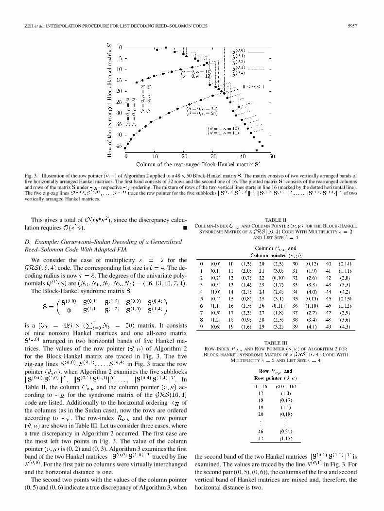
Fig. 3. Illustration of the row pointer �� of Algorithm 2 applied to a 48� 50 Block-Hankel matrix �. The matrix consists of two vertically arranged bands offive horizontally arranged Hankel matrices. The first band consists of 32 rows and the second one of 16. The plotted matrix � consists of the rearranged columnsand rows of the matrix � under� - respective� -ordering. The mixture of rows of the two vertical lines starts in line 16 (marked by the dotted horizontal line).The five zig-zag lines � � � � � � � � � trace the row pointer for the five subblocks �� of twovertically arranged Hankel matrices.

This gives a total of , since the discrepancy calcu-lation requires .

D. Example: Guruswami–Sudan Decoding of a GeneralizedReed–Solomon Code With Adapted FIA

We consider the case of multiplicity for thecode. The corresponding list size is . The de-

coding radius is now . The degrees of the univariate poly-nomials are .

The Block-Hankel syndrome matrix

is a matrix. It consistsof nine nonzero Hankel matrices and one all-zero matrix

arranged in two horizontal bands of five Hankel ma-trices. The values of the row pointer of Algorithm 2for the Block-Hankel matrix are traced in Fig. 3. The fivezig-zag lines in Fig. 3 trace the rowpointer , when Algorithm 2 examines the five subblocks

. InTable II, the column and the column pointer ac-cording to for the syndrome matrix of thecode are listed. Additionally to the horizontal ordering ofthe columns (as in the Sudan case), now the rows are orderedaccording to . The row-index and the row pointer

are shown in Table III. Let us consider three cases, wherea true discrepancy in Algorithm 2 occurred. The first case arethe most left two points in Fig. 3. The value of the columnpointer is (0, 2) and (0, 3). Algorithm 3 examines the firstband of the two Hankel matrices traced by line

. For the first pair no columns were virtually interchangedand the horizontal distance is one.

The second two points with the values of the column pointer(0, 5) and (0, 6) indicate a true discrepancy of Algorithm 3, when

TABLE IICOLUMN-INDEX � AND COLUMN POINTER �� FOR THE BLOCK-HANKEL

SYNDROME MATRIX OF A �� CODE WITH MULTIPLICITY � � �AND LIST SIZE � �

TABLE IIIROW-INDEX AND ROW POINTER �� OF ALGORITHM 2 FOR

BLOCK-HANKEL SYNDROME MATRIX OF A �� CODE WITH

MULTIPLICITY � � � AND LIST SIZE � �

the second band of the two Hankel matrices isexamined. The values are traced by the line in Fig. 3. Forthe second pair ((0, 5), (0, 6)), the columns of the first and secondvertical band of Hankel matrices are mixed and, therefore, thehorizontal distance is two.


The third considered case, where a true discrepancy occurs,are the most right two points in Fig. 3 indicated by values (1, 10)and (1, 11) of the row pointer . Algorithm 2 examines theband of the two Hankel matrices and restarts(at the point (1, 10)) with the previous stored value of the rowpointer (at (1, 11)). In between four other horizontal bands ofmatrices were examined.

VI. CONCLUSION

We reformulated the Guruswami–Sudan interpolation con-ditions (for a multiplicity higher than one) for GeneralizedReed–Solomon codes into a set of univariate polynomialequations, which can partially be seen as Extended Key Equa-tions. The obtained set of homogeneous linear equations has aBlock-Hankel structure. We adapted the Fundamental IterativeAlgorithm of Feng and Tzeng to this special structure andachieved a significant reduction of the time complexity.

As mentioned in Note 2, the set of equations can be furtherreduced, under the observation that the diagonal terms areconstant, i.e., they do not depend on the received word. Thisreduction leads to a loss of the Block-Hankel structure andtherefore would destroy the quadratic complexity. We notethat Beelen and Høholdt [34] mentioned this reduction for theGuruswami–Sudan interpolation step for Algebraic Geometriccodes, to get a smaller interpolation problem, but the systemdoes not appear to be Block-Hankel.

We conclude that we identified the quantity (seeNote 2) without having found an interpretation of that number.

ACKNOWLEDGMENT

The authors thank V. Sidorenko and M. Bossert for fruitfuldiscussions. They thank the anonymous referees for their valu-able comments that improved the presentation of this paper.

REFERENCES

[1] D. Augot and A. Zeh, “On the Roth and Ruckenstein equations for theGuruswami–Sudan algorithm,” in Proc. IEEE Int. Symp. Inf. Theory(ISIT 2008), 2008, pp. 2620–2624 [Online]. Available: http://dx.doi.org/10.1109/ISIT.2008.4595466

[2] A. Zeh, C. Gentner, and M. Bossert, “Efficient list-decoding ofReed–Solomon codes with the fundamental iterative algorithm,” inProc. Inf. Theory Workshop (ITW 2009), Oct. 2009 [Online]. Avail-able: http://dx.doi.org/10.1109/ITW.2009.5351241

[3] V. Guruswami and M. Sudan, “Improved decoding of Reed–Solomonand algebraic-geometry codes,” IEEE Trans. Inf. Theory vol. 45, no.6, pp. 1757–1767, 1999 [Online]. Available: http://ieeexplore.ieee.org/xpls/abs_all.jsp?arnumber=782097

[4] V. Guruswami, List Decoding of Error-Correcting Codes, ser. LectureNotes in Computer Science. New York: Springer, 2004, no. 3282.

[5] V. Guruswami, Algorithmic Results in List Decoding. New York:Now, Jan. 2007.

[6] M. Sudan, “Decoding of Reed–Solomon codes beyond the error-cor-rection bound,” J. Complex. vol. 13, no. 1, pp. 180–193, Mar. 1997[Online]. Available: http://dx.doi.org/10.1006/jcom.1997.0439

[7] I. S. Reed and G. Solomon, “Polynomial codes over certain finitefields,” J. Soc. Indust. Appl. Math. vol. 8, no. 2, pp. 300–304, 1960[Online]. Available: http://dx.doi.org/10.1137/0108018

[8] R. Koetter, “On algebraic decoding of algebraic-geometric and cycliccodes,” Ph.D. dissertation, Univ. Linköping, , 1996.

[9] R. M. Roth and G. Ruckenstein, “Efficient decoding of Reed–Solomoncodes beyond half the minimum distance,” IEEE Trans. Inf. Theory vol.46, no. 1, pp. 246–257, 2000 [Online]. Available: http://ieeexplore.ieee.org/xpls/abs_all.jsp?arnumber=817522

[10] G. Ruckenstein, “Error decoding strategies for algebraic codes” Ph.D.dissertation, The Technion, Haifa, Israel, 2001 [Online]. Available:http://www.cs.technion.ac.il/users/wwwb/cgi-bin/tr-info.cgi/2001/PHD/PHD-2001-01

[11] M. Alekhnovich, “Linear diophantine equations over polynomials andsoft decoding of Reed–Solomon codes,” IEEE Trans. Inf. Theory vol.51, no. 7, pp. 2257–2265, 2005 [Online]. Available: http://ieeexplore.ieee.org/xpls/abs_all.jsp?arnumber=1459042

[12] P. Trifonov, “Efficient interpolation in the Guruswami–Sudan al-gorithm,” IEEE Trans. Inf. Theory vol. 56, no. 9, pp. 4341–4349,Sep. 2010 [Online]. Available: http://dx.doi.org/10.1109/TIT.2010.2053901

[13] S. Sakata, H. F. Mattson, T. Mora, and T. R. N. Rao, Eds., “Findinga minimal polynomial vector set of a vector of nD arrays,” in Proc.Appl. Algebra, Algebraic Algorithms and Error-Correcting Codes(AAECC’91), Berlin, Germany, Oct. 1991, vol. 539, pp. 414–425[Online]. Available: http://dx.doi.org/10.1007/3-540-54522-0_129,ser. LNCS, Springer, [Online]. Available:

[14] S. Sakata, “On fast interpolation method for Guruswami–Sudan list de-coding of one-point algebraic-geometry codes,” in Applied Algebra, Al-gebraic Algorithms and Error-Correcting Codes, ser. Lecture Notes inComput. Sci., S. Boztas and I. E. Shparlinski, Eds. Berlin, Germany:Springer, Oct. 2001, vol. 2227, ch. 18, pp. 172–181 [Online]. Avail-able: http://dx.doi.org/10.1007/3-540-45624-4_18

[15] G. L. Feng and K. K. Tzeng, “A generalization of the Berlekamp-Massey algorithm for multisequence shift-register synthesis with ap-plications to decoding cyclic codes,” IEEE Trans. Inf. Theory vol. 37,no. 5, pp. 1274–1287, 1991 [Online]. Available: http://ieeexplore.ieee.org/xpls/abs_all.jsp?arnumber=133246

[16] E. R. Berlekamp, Algebraic Coding Theory. New York: McGraw-Hill, 1968.

[17] J. Massey, “Shift-register synthesis and BCH decoding,” IEEE Trans.Inf. Theory vol. 15, no. 1, pp. 122–127, Jan. 2003 [Online]. Available:http://ieeexplore.ieee.org/xpls/abs_all.jsp?arnumber=1054260

[18] P. Beelen and T. Høholdt, “A syndrome formulation of the interpola-tion step in the Guruswami–Sudan algorithm,” in ICMCTA, ser. Lec-ture Notes in Comput. Sci., A. I. Barbero, Ed. New York: Springer,2008, vol. 5228, pp. 20–32 [Online]. Available: http://dx.doi.org/10.1007/978-3-540-87448-5_3

[19] P. Beelen and K. Brander, “Key equations for list decoding ofReed–Solomon codes and how to solve them,” J. Symbol. Computat.,vol. 45, no. 7, pp. 773–786, Jul. 2010.

[20] E. R. Berlekamp and L. Welch, “Error Correction of Algebraic BlockCodes,” U.S. Patent Number 4 633 470.

[21] F. J. MacWilliams and N. J. A. Sloane, The Theory of Error-CorrectingCodes (North-Holland Mathematical Library). Amsterdam: NorthHolland, Jun. 1988.

[22] R. Roth, Introduction to Coding Theory. Cambridge, U.K.: Cam-bridge Univ. Press, Mar. 2006.

[23] H. Hasse, “Theorie der höheren Differentiale in einem algebraischenFunktionenkörper mit vollkommenem Konstantenkörper bei beliebigerCharakteristik,” J. Reine Angew. Math., vol. 175, pp. 50–54, 1936.

[24] P. Gemmell and M. Sudan, “Highly resilient correctors for polyno-mials,” Inf. Process. Lett., vol. 43, no. 4, pp. 169–174, Sep. 1992.

[25] T. Yaghoobian and I. F. Blake, “Two new decoding algorithms forReed–Solomon codes,” Applicable Algebra in Eng., Commun. Comput.vol. 5, no. 1, pp. 23–43, Jan. 1994 [Online]. Available: http://dx.doi.org/10.1007/BF01196623

[26] D. Dabiri and I. F. Blake, “Fast parallel algorithms for decodingReed–Solomon codes based on remainder polynomials,” IEEE Trans.Inf. Theory vol. 41, no. 4, pp. 873–885, 1995 [Online]. Available:http://dx.doi.org/10.1109/18.391235

[27] J. Justesen and T. Hoholdt, A Course in Error-Correcting Codes (EMSTextbooks in Mathematics). Zürich, Switzerland: Eur. Math. Soc.,Feb. 2004.

[28] Y. Sugiyama, M. Kasahara, S. Hirasawa, and T. Namekawa, “A methodfor solving key equation for decoding goppa codes,” Inf. Contr., vol. 27,no. 1, pp. 87–99, 1975.

[29] J. Dornstetter, “On the equivalence between Berlekamp’s and Euclid’salgorithms,” IEEE Trans. Inf. Theory vol. 33, no. 3, pp. 428–431, 1987[Online]. Available: http://ieeexplore.ieee.org/xpls/abs_all.jsp?ar-number=1057299

[30] A. E. Heydtmann and J. M. Jensen, “On the equivalence of theBerlekamp-Massey and the Euclidean algorithms for decoding,” IEEETrans. Inf. Theory vol. 46, no. 7, pp. 2614–2624, 2000 [Online].Available: http://dx.doi.org/10.1109/18.887869


[31] M. Bras-Amorós and M. E. O’Sullivan, “From the Euclidean algo-rithm for solving a key equation for dual Reed–Solomon codes tothe Berlekamp-Massey algorithm,” in AAECC, ser. Lecture Notesin Computer Science, M. Bras-Amorós and T. Høholdt, Eds. NewYork: Springer, 2009, vol. 5527, pp. 32–42 [Online]. Available:http://dx.doi.org/10.1007/978-3-642-02181-7

[32] G. Schmidt, V. R. Sidorenko, and M. Bossert, “Collaborative decodingof interleaved Reed–Solomon codes and concatenated code designs,”IEEE Trans. Inf. Theory vol. 55, no. 7, pp. 2991–3012, 2009 [Online].Available: http://dx.doi.org/10.1109/TIT.2009.2021308

[33] R. J. Mceliece, The Guruswami–Sudan Decoding Algorithm forReed–Solomon Codes Interplanetary Netw. Progress Rep., Jan. 2003,vol. 153, pp. 1–60 [Online]. Available: http://ipnpr.jpl.nasa.gov/progress_report/42-153/153F.pdf

[34] P. Beelen and T. Hoholdt, “The decoding of algebraic geometrycodes,” in Series on Coding Theory and Cryptology: Advances inAlgebraic Geometry Codes. New York: World Scientific, 2008, vol.5, pp. 49–98.

Alexander Zeh (S’09) received the Dipl.-Ing.(BA) degree in 2004 in electricalengineering with the main topic automation technology from the Universityof Applied Science (Berufsakademie) Stuttgart, Stuttgart, Germany, and theDipl.-Ing. degree in 2008 in electrical engineering from the University ofStuttgart, Stuttgart, Germany. He participated in the double-diploma programwith Télécom ParisTech (former ENST) from 2006 to 2008 and received aFrench diploma.

Currently he is a Ph.D. student with the Institute of Telecommunications andApplied Information Theory, University of Ulm, Germany, and with the Com-puter Science Department (LIX), École Polytechnique ParisTech, Paris, France.His current research interests include coding and information theory, signalprocessing, telecommunications, and the implementation of fast algorithms onFPGAs.

Christian Gentner (M’10) received the Dipl.-Ing.(BA) degree in 2006 in elec-trical engineering with the main topic communication technology from the Uni-versity of Applied Science (Berufsakademie) Ravensburg, Ravensburg, Ger-many, and the M.Sc. degree in telecommunication and media technology in2009, from the University of Ulm, Ulm, Germany.

He is currently working toward the Ph.D. degree with the Institute of Com-munications and Navigation of the German Aerospace Center (DLR), Germany.His current research interests include multisensor navigation, propagation ef-fects and nonline-of-sight identification and mitigation, as well as the imple-mentation of these algorithms on FPGAs.

Daniel Augot received the Masters degree in theoretical computer science in1989 from the University Pierre and Marie Curie, Paris VI, Paris, France. Hewas a Ph.D. student of Pascale Charpin and graduated in 1993 at the UniversityPierre and Marie Curie, Paris VI, Paris, France.

He was then hired as a Researcher at INRIA-Rocquencourt. In 2009, he be-came a Senior Researcher with INRIA—Saclay-Île-de-France and École Poly-technique. His major research interests are coding theory, cryptography, andtheir interplay.

Documents

5946 IEEE TRANSACTIONS ON INFORMATION …elib.dlr.de/72163/1/10.1.1.220.6721(1).pdf5946 IEEE TRANSACTIONS ON INFORMATION THEORY, VOL. 57, NO. 9, SEPTEMBER 2011 An Interpolation Procedure