582487 Data Compression Techniques

Lecture 3: Integer Codes I

Simon J. Puglisi (puglisi@cs.helsinki.fi)

University of Helsinki Department of Computer Science

Outline

•  Motivation: why integer codes?

•  This week: three classic flavors –  Unary –  Elias codes (gamma, delta) –  Golomb codes (Rice, general)

•  Thursday: three modern flavours –  Interpolative binary codes –  Variable-byte codes –  Word-aligned binary codes (simple, relative, carryover)

Integer codes

•  Today: variable length codes for integers. We want a prefix code when the source alphabet is N, the set of natural numbers

•  We cannot use the Huffman algorithm or anything similar on an infinite alphabet. Often there is an upperbound on the integers, but even then the alphabet can be too large to compute and store the Huffman code efficiently.

•  Also, although we can decode Huffman codes fast in theory, in practice decoding Huffman codes requires table lookups, which are slow.

Integer codes

•  As an alternative to Huffman, we have a number of integer codes that are (usually) fixed codes for encoding all natural numbers.

•  With each of them, the codeword length is a non-decreasing function of the integer value. i.e. Smaller numbers get shorter codes. The schemes differ on how fast the growth is.

•  The codes described in this lecture are for all non-negative integers excluding zero. Including zero is usually easy.

How does Google work?

How does Google work?

•  Crawl the web, gather a collection of documents

•  For each word t in the collection, store a list of all documents containing t:

•  Query: blue mittens

blue

blunt

mittens

…

1 2 4 11 31 45 173

1 2 4 5 6 16 57 132 173 …

…

174

lexicon postings

…

…

mint 2 31 54 101

1 4 5 11 31 45 174 288

Inverted Index

How does Google work?

•  Query: blue mittens

blue

mittens

1 2 4 11 31 45 173 174

1 4 5 11 31 45 174 288

Intersect lists 1 4 11 31 45 174

Why does Google use compression?

•  We can compress both components of an inverted index

•  Today: techniques for compressing the lists –  Lists much bigger than lexicon (factor 10 at least) –  (stuff for lexicon compression later in the course)

•  Motivation: if we don’t compress the lists we’ll have to store

them on disk because they’re enormous

•  Compression allows us to keep them (or most of them) in memory. If decompressing in memory is faster than reading from disk we get a saving. This is the case with int codes.

•  Even if we still have to store some lists on disk, storing them compressed means we can read them into memory faster at intersection time

•  Consider the following list in an inverted index:

L = 3,7,11,23,29,37,41,… •  Compressing L directly, with, say, Huffman coding, is

not feasible: the number of elements in the list can be very large, and each element is unique

•  Elements (doc ids) are repeated across lists –  document D with m distinct words appears in m different lists –  …but we still don’t want to use Huffman... –  …it requires lookups, and these are slow. And for compression

to be worthwhile we need decompression to be fast. –  We need codes that are local.

Use Huffman?

•  The key idea for compressing inverted lists is to observe that elements of L are monotonically increasing, so we can transform the list by taking differences (gaps):

L = 3,7,11,23,29,37,41,…

D(L) = 3,4,4,12,6,8,4,…

•  The advantage of doing this is to make the integers smaller, and suitable for integer codes –  Remember we said smaller integers get smaller codes

•  We can easily “degap” the list during intersection –  Adding items together as we scan the lists adds little overhead

Gap Encoding

inverted list

the docIDs … 283042 283043 283044 283045 …

gaps … 1 1 1 …

computer docIDs … 283047 283154 283159 283202 …

gaps … 107 5 43 …

arachnid docIDs 252000 500100

gaps 252000 248100

Variable Length Encoding

What we want: –  For arachnid and other rare terms: use about 20

bits per gap (= integer). –  For the and other very frequent terms: use about 1

bit per gap (= integer).

Integer representations…

Binary codes

•  binaryk(n) = binary representation of an integer n using k-bits.

•  binary4(13) = 1101, binary7(13) = 0001101

•  Idea for encoding integers: just use minimal binary codes! –  After all, that’s small…

★minimal binary code for 13

Just use binary representations…?

•  283154, 5, 43, 3

•  1000101001000010010, 101, 101011, 11

•  100010100100001001010110101111 –  Uhhh…

•  We have to be able to decompress as well! –  Our coding scheme must be prefix free –  We need a prefix code

Unary codes

•  Our first proper prefix code is the unary code

•  Represents integer n as n-1 ‘1’s with a final ‘0’. –  So the unary code for integer n has length n. –  (Note: we could reverse the roles of 0s and 1s)

•  Unary code for 3 is 110.

•  Unary code for 40 is 1111111111111111111111111111111111111110.

Digression…

•  What is the Huffman code for the probability distribution: 1/2,1/4,1/8,1/16,...

•  So unary codes are optimal sometimes…

...

1

1

1

10

0

0

0

0

10

110

1110

Unary codes

•  The unary code is optimal if the integers to be encoded follow a geometric distribution of the form: Pr(i) = (½)i

•  Pretty specific.

•  Nonetheless unary codes play an important role in the design of other codes.

Elias codes…

Elias γ codes

•  Our first non-trivial integer code is the γ (gamma) code, discovered by Peter Elias in 1975.

•  Represent an integer n > 0 as a pair of selector and offset.

•  Offset is the integer in binary, with the leading bit chopped off. –  For example 13 → 1101 → 101

•  Selector is the length of offset + 1. –  For 13 (offset 101), this is 3 + 1 = 4. –  Encode selector in unary code: 1110.

•  Gamma code of 13 is the concatenation of selector & offset: –  1110, 101 = 1110101.

Elias γ codes

•  Thinking back, the problem with our earlier “brain wave” of just using the minimal binary representations was that, later, we didn’t know the length of each code

4, 43, 3 became 10110101111

•  γ codes solve that problem by prefixing the minimal binary code with an unambiguous representation of the length (a unary representation)

1101001111101010111011

•  There is also a further optimization present…

Elias γ codes

•  …the most significant bit of the minimal binary code is always 1. So we don’t need to store it.

1110101111111010101111011

1110101111111010101111011 •  It is tempting to now try and reduce the selectors

1110101111111010101111011

1100111111001011101

•  …but we shouldn’t. Why?

Gamma code examples

number binary rep selector offset γ code

1 1 0 0

2 10 10 0 10,0

3 11 10 1 10,1

4 100 110 00 110,00

9 1001 1110 001 1110,001

13 1101 1110 101 1110,101

24 11000 11110 1000 11110,1000

511 11111111 111111110 11111111 111111110, 11111111

1025 10000000001 11111111110 0000000001 11111111110, 0000000001

Decoding a Gamma ray

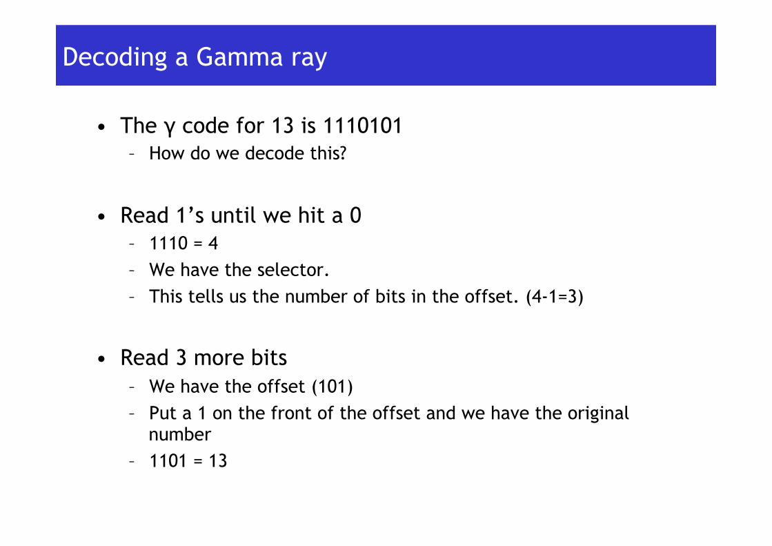
•  The γ code for 13 is 1110101 –  How do we decode this?

•  Read 1’s until we hit a 0 –  1110 = 4 –  We have the selector. –  This tells us the number of bits in the offset. (4-1=3)

•  Read 3 more bits –  We have the offset (101) –  Put a 1 on the front of the offset and we have the original

number –  1101 = 13

Decoding a Gamma ray

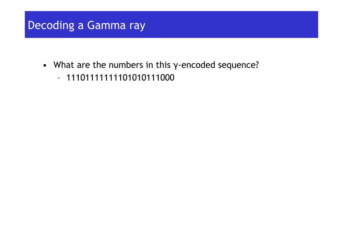
•  What are the numbers in this γ-encoded sequence? –  11101111111101010111000

Length of a Gamma code

•  The length of offset is bits.

•  The length of selector is bits,

•  So the length of the entire code is bits. –  So γ codes are always of odd length.

•  γ codes are just over twice the size of the minimal binary code

2 !"#! ! + 1!!"#! ! + 1!!"#! ! !

Nice things…

•  The γ code is parameter-free.

•  Optimal for integer sequences that follow the probability distribution: Pr(n) = 1/(2n2)

Elias δ codes

•  γ coding works well when the integers to be compressed as small (say, < 32), but they are quite wasteful on bigger integers

•  In such situations the δ (delta) code – also invented by Elias – may be a better choice.

•  δ codes are like γ code, but represent length as a γ code instead of a unary code –  What are the γ and δ codes for 7? –  What about for 68?

Nice things about δ codes

•  Compared with γ coding, where the length of the codeword for an integer n is about 2logn, the δ code for the same integer consumes only:

bits.

•  Optimal when the integers to be compressed conform to the following probability distribution: Pr[n] = 1/(2n(logn)2)

!(!) = !"#! ! + !2 !"#! !"#! ! + 1 + 1!

Elias ω codes

•  Elias also described ω (omega) codes –  Similar idea to δ codes, but length is recursively

encoded

Golomb codes…

Golomb codes

•  Invented by Solomon Golomb in 1966.

•  Unlike Elias codes, Golomb codes are parametric: they take a single (integer) parameter M, the modulus.

•  We’ll start with a special (and useful) case called Rice codes, where M is restricted to be a power of 2.

Golomb-Rice codes

•  Choose an integer M = 2j, the modulus.

•  We want to encode the integer n > 0. Split n into two components, the quotient q(n) and the remainder r(n):

q(n) = ((n-1)/M) r(n) = (n-1) mod M

•  Encode n by writing: q(n)+1 in unary, followed by r(n) as a logM-bit binary number*

Example

•  q(n) = floor(n-1/M), r(n) = (n-1) mod M –  GolombRice(n) = unary(q(n)+1) . binary(logM)r(n)

•  Let M = 27 and n = 345; •  then GolombRice(345) = 110 1011000, since

q(345) = (345-1)/27 = 2, and r(345) = (345-1) mod 27 = 88.

Decoding…

•  q(n) = floor(n-1/M), r(n) = (n-1) mod M –  GolombRice(n) = unary(q(n)+1) . binary(logM)r(n)

•  Decoding is straightforward:

–  q(n)+1 is encoded in unary, so q(n) is easily found –  and the decoder knows M, so knows to extract the next

logM bits as r(n) –  … then it’s just a matter of reversing the arithmetic

n = q(n)�M + r(n) + 1

•  If M is 8, what is 1110110?

Visualizing Golomb(-Rice) codes

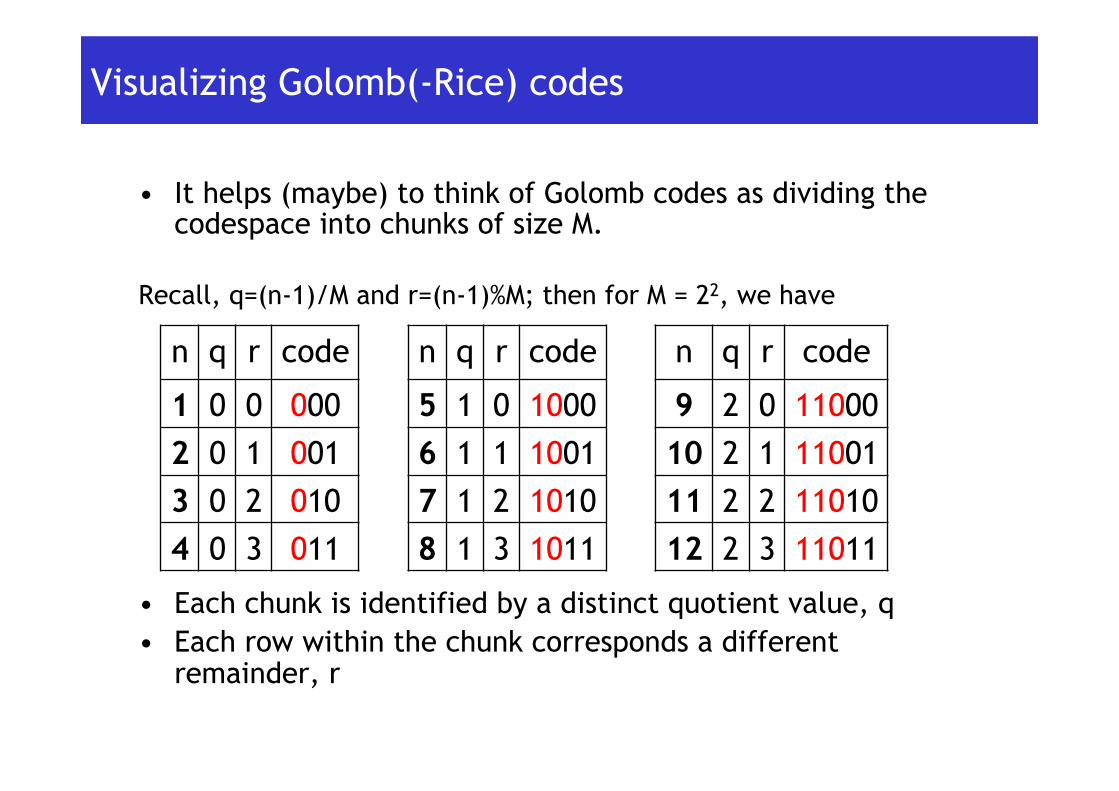
•  It helps (maybe) to think of Golomb codes as dividing the codespace into chunks of size M.

Recall, q=(n-1)/M and r=(n-1)%M; then for M = 22, we have

•  Each chunk is identified by a distinct quotient value, q •  Each row within the chunk corresponds a different

remainder, r

n q r code

1 0 0 000 2 0 1 001 3 0 2 010 4 0 3 011

n q r code

5 1 0 1000 6 1 1 1001 7 1 2 1010 8 1 3 1011

n q r code

9 2 0 11000 10 2 1 11001 11 2 2 11010 12 2 3 11011

General modulus

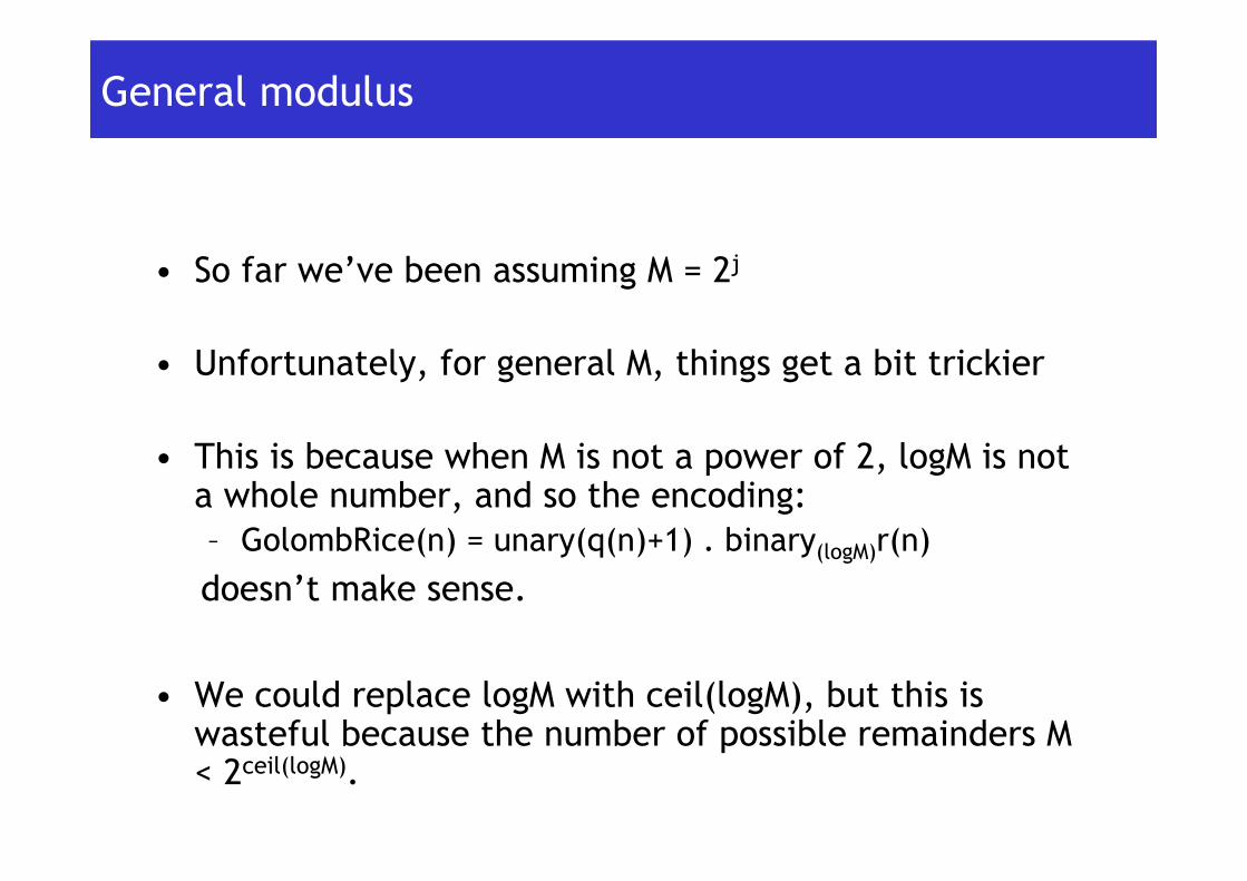
•  So far we’ve been assuming M = 2j

•  Unfortunately, for general M, things get a bit trickier

•  This is because when M is not a power of 2, logM is not a whole number, and so the encoding: –  GolombRice(n) = unary(q(n)+1) . binary(logM)r(n)

doesn’t make sense.

•  We could replace logM with ceil(logM), but this is wasteful because the number of possible remainders M < 2ceil(logM).

General Golomb codes

•  A naïve and wasteful encoding with M=6

•  Ideally we would be using logM = 2.5849… bits per r encoding •  Here we’re using ceil(logM) = 3

n q r code

1 0 0 0001 2 0 1 0011 3 0 2 0010 4 0 3 0011 5 0 4 0100 6 0 5 0101

Optimal encoding for general modulus

•  The trick is to encode some of the remainders in shorter floor(logM)-bit code words, and others using ceil(logM)-bit code words.

•  In particular, values from the interval [0, 2ceil(logM)-M-1] receive the shorter code words, longer code words go to [2ceil(logM)-M, 2ceil(logM)-1].

•  For M=6 this means remainders 0 and 1 get a 2-bit code, while 2, 3, 4, and 5 each get 3-bit codes

General Golomb codes

•  Optimal encoding with M=6

•  Ideally we would be using logM = 2.5849… bits per r encoding •  Here we’re using ceil(logM) = 3 •  Now the average is 2.66…, which is much better.

n q r code

1 0 0 0001 2 0 1 0011 3 0 2 0010 4 0 3 0011 5 0 4 0100 6 0 5 0101

n q r code

1 0 0 000 2 0 1 001 3 0 2 0100 4 0 3 0101 5 0 4 0110 6 0 5 0111

Nice things about Golomb codes

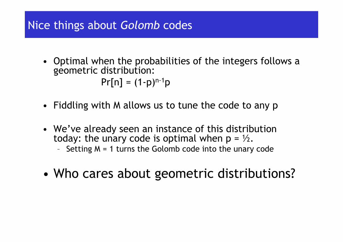
•  Optimal when the probabilities of the integers follows a geometric distribution:

Pr[n] = (1-p)n-1p

•  Fiddling with M allows us to tune the code to any p •  We’ve already seen an instance of this distribution

today: the unary code is optimal when p = ½. –  Setting M = 1 turns the Golomb code into the unary code

• Who cares about geometric distributions?

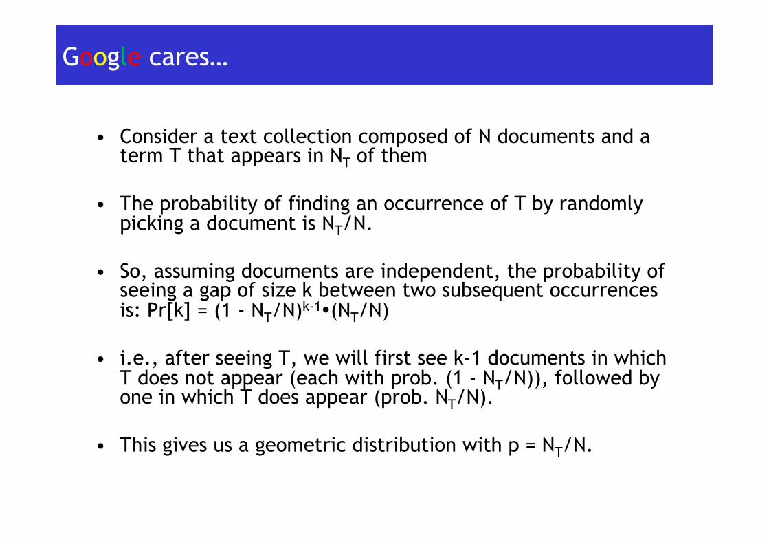
•  Consider a text collection composed of N documents and a term T that appears in NT of them

•  The probability of finding an occurrence of T by randomly picking a document is NT/N.

•  So, assuming documents are independent, the probability of seeing a gap of size k between two subsequent occurrences is: Pr[k] = (1 - NT/N)k-1�(NT/N)

•  i.e., after seeing T, we will first see k-1 documents in which T does not appear (each with prob. (1 - NT/N)), followed by one in which T does appear (prob. NT/N).

•  This gives us a geometric distribution with p = NT/N.

Google cares…

Summary

•  Integer codes are neat little things

•  Not as general as Huffman, but are much more lightweight.

•  In effect, they get around Huffman’s complexity by targeting (i.e. assuming) a particular distribution –  Huffman will produce an optimal code for any distribution

Alignment…

•  Machine memory has natural boundaries – 8, 32, 64 bits –  (bytes and words)

•  Compressing and manipulating at individual bit-granularity – as in the codes we have seen today – can be slow

•  Next lecture we’ll look at integer codes that respect byte and word boundaries… and other codes that try to exploit clustering present in the stream of integers being compressed…

Next lecture…

13/01 Shannon’s Theorem 15/01 Huffman Coding 20/01 Integer Codes I 22/01 Integer Codes II 27/01 Dynamic Prefix Coding 29/01 Arithmetic Coding 03/02 Text Compression 05/02 No Lecture 10/02 Text Compression 12/02 Compressed Data Structures 17/02 Compressed Data Structures 19/02 Compressed Data Structures 24/02 Compressed Data Structures