580.691 Learning Theory

Reza Shadmehr

Bayesian Learning 2:

Gaussian distribution & linear regression

Causal inference

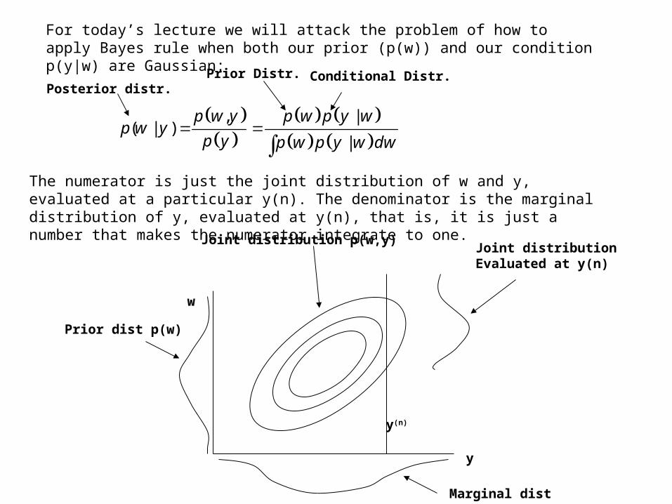
The numerator is just the joint distribution of w and y, evaluated at a particular y(n). The denominator is the marginal distribution of y, evaluated at y(n), that is, it is just a number that makes the numerator integrate to one.

For today’s lecture we will attack the problem of how to apply Bayes rule when both our prior (p(w)) and our condition p(y|w) are Gaussian:

, |( | )

|

p w y p w p y wp w y

p y p w p y w dw

Posterior distr.Prior Distr. Conditional Distr.

w

y

y(n)

Prior dist p(w)

Marginal dist p(y)

Joint distributionEvaluated at y(n)

Joint distribution p(w,y)

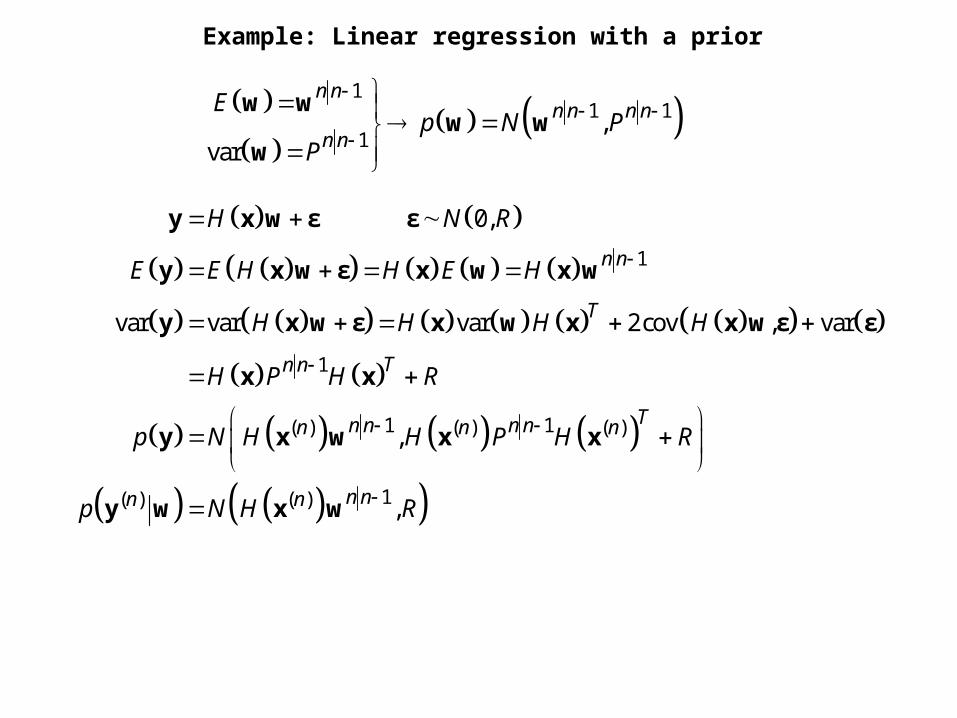
Example: Linear regression with a prior

1

1

1 1( ) ( ) ( )

1( ) ( )

0,

var var var 2cov , var

,

,

n n

T

Tn n

Tn n n nn n n

n nn n

H N R

E E H H E H

H H H H

H P H R

p N H H P H R

p N H R

y x w ε ε

y x w ε x w x w

y x w ε x w x x w ε ε

x x

y x w x x

y w x w

1

1 1

1,

var

n nn n n n

n n

Ep N P

P

w ww w

w

1

1 1 1

1( ) 1 1

cov , cov ,

var( )

, ,

T

T T TT T T

TT

n n

n n Tn n n n

n nn Tn n n n

H E H H E E

E H H E H E H E E E

H E H E E

H H P

P P Hp p N

H H P H P H

y w x w ε w x w ε x w w w

x ww x w w x w w x w w εw ε w

x ww x w w

x w x

w xww y

y x w x x x

1 11 12

2 21 22,

R

N

μ

μ

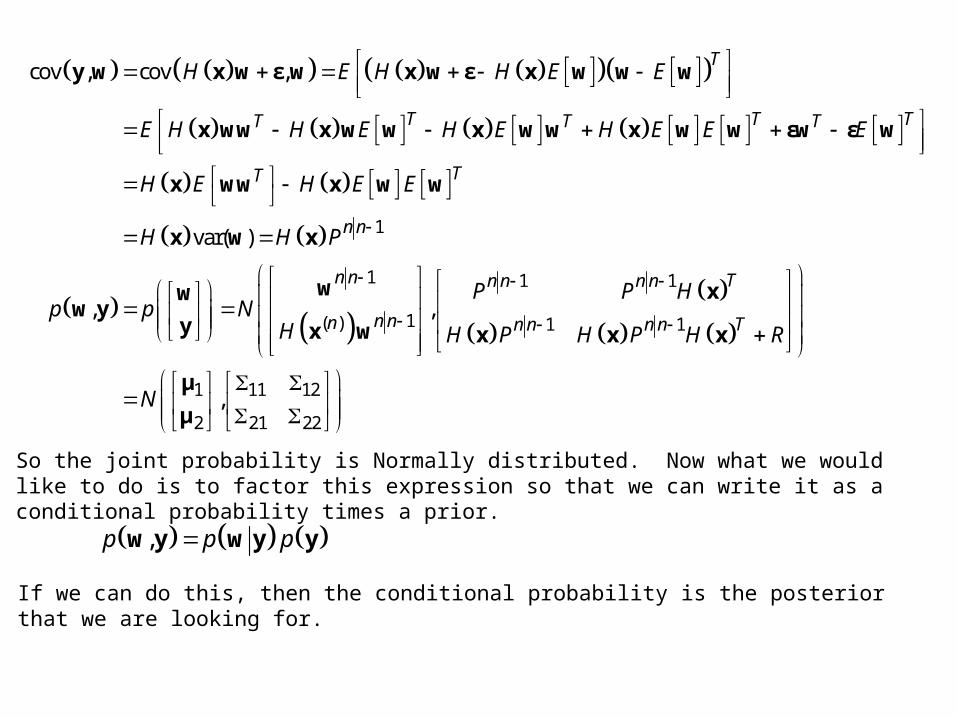
So the joint probability is Normally distributed. Now what we would like to do is to factor this expression so that we can write it as a conditional probability times a prior.

,p p pw y w y y

If we can do this, then the conditional probability is the posterior that we are looking for.

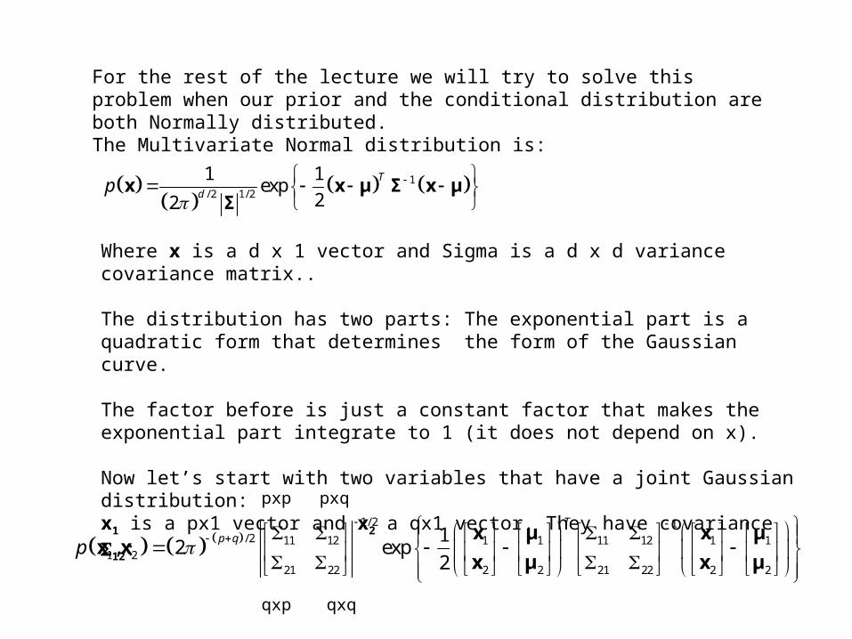
For the rest of the lecture we will try to solve this problem when our prior and the conditional distribution are both Normally distributed.The Multivariate Normal distribution is:

11/ 2/ 2

1 1exp

22

T

dp

x x μ Σ x μΣ

Where x is a d x 1 vector and Sigma is a d x d variance covariance matrix..

The distribution has two parts: The exponential part is a quadratic form that determines the form of the Gaussian curve.

The factor before is just a constant factor that makes the exponential part integrate to 1 (it does not depend on x).

Now let’s start with two variables that have a joint Gaussian distribution:x1 is a px1 vector and x2 a qx1 vector. They have covariance 12:

1/ 2 1

/ 2 11 12 1 1 11 12 1 11 2

21 22 2 2 21 22 2 2

1, 2 exp

2

T

p qp

x μ x μx x

x μ x μ

pxp pxq

qxqqxp

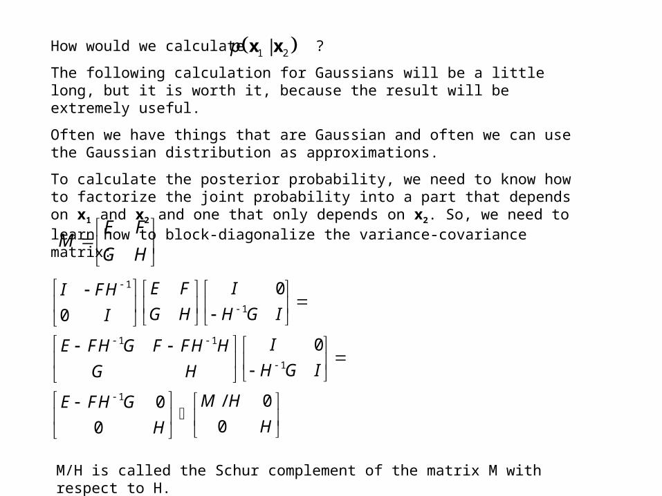
How would we calculate ?

The following calculation for Gaussians will be a little long, but it is worth it, because the result will be extremely useful.

Often we have things that are Gaussian and often we can use the Gaussian distribution as approximations.

To calculate the posterior probability, we need to know how to factorize the joint probability into a part that depends on x1 and x2 and one that only depends on x2. So, we need to learn how to block-diagonalize the variance-covariance matrix:

1 2|p x x

E FM

G H

1

1

1 1

1

1

0

0

0

/ 00

00

E F II FH

G H H G II

IE FH G F FH H

H G IG H

M HE FH G

HH

M/H is called the Schur complement of the matrix M with respect to H.

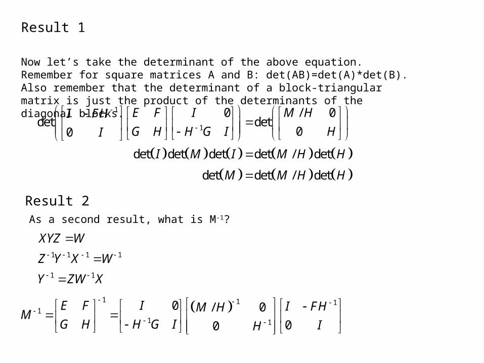
Now let’s take the determinant of the above equation. Remember for square matrices A and B: det(AB)=det(A)*det(B). Also remember that the determinant of a block-triangular matrix is just the product of the determinants of the diagonal blocks.

1

1

0 / 0det det

00

det det det det / det

det det / det

E F I M HI FH

G H H G I HI

I M I M H H

M M H H

As a second result, what is M-1?

1 1 1 1

1 1

XYZ W

Z Y X W

Y ZW X

1 1 11

1 1

0 / 0

00

E F I I FHM HM

G H H G I IH

Result 1

Result 2

1/ 2

/ 2 11 12

21 22

1/ 2/1//

2

2 2

2

2

222 / 2

2

p q

p q

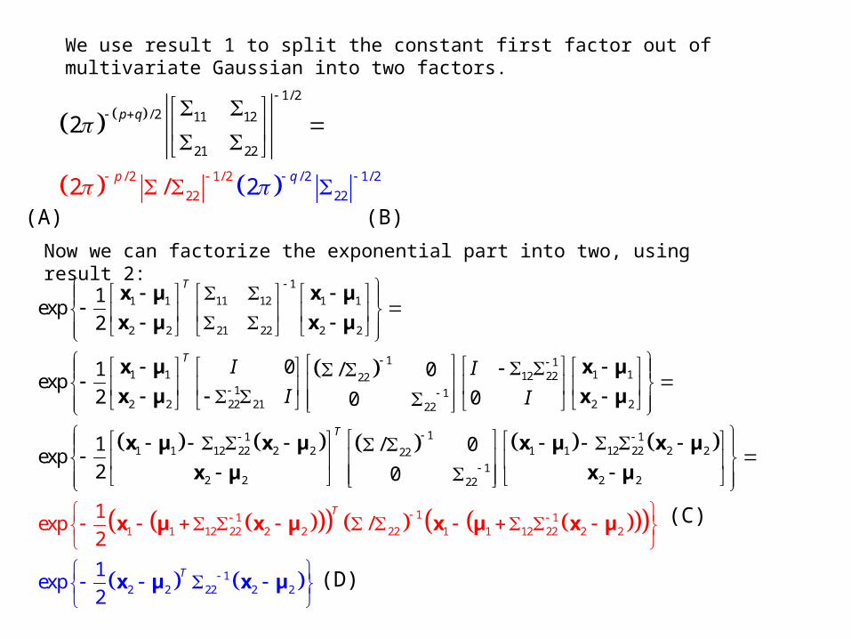
We use result 1 to split the constant first factor out of multivariate Gaussian into two factors.

Now we can factorize the exponential part into two, using result 2:

1

1 1 11 12 1 1

2 2 21 22 2 2

1 11 1 1 112 2222

1 12 2 22 21 2 222

11 1 12 22 2

1exp

2

01 / 0exp

2 00

1exp

2

T

TI I

I I

x μ x μ

x μ x μ

x μ x μ

x μ x μ

x μ x

11 11 1 12 22 2 2 22

12 2 22

1 1 12 22

1 12

2 2

1 1 12 22 2 2221

2 2 2 2

2

22

2

1exp /

/ 0

1ex

2

2

0

pT

T

T

μ x μ x μ

x μ x μ

x μ x μ x μ

μ

x

μ

μ

x x

(A) (B)

(C)

(D)

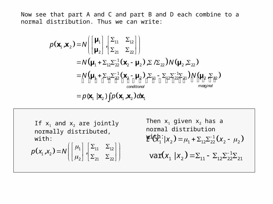
Now see that part A and C and part B and D each combine to a normal distribution. Thus we can write:

1 11 121 2

2 21 22

11 12 22 2 2 22 2 22

1 11 12 22 2 2 11 12 22 21 2 22

arg

1 2 1 2 1

, ,

, / ,

, ,

( | ) ,

m inalconditional

p N

N N

N N

p p d

μx x

μ

μ x μ μ

μ x μ μ

x x x x x

1 11 121 2

2 21 22

, ,p x x N

1

1 2 11 12 22 21var |x x

11 2 1 12 22 2 2|E x x x

If x1 and x2 are jointly normally distributed, with:

Then x1 given x2 has a normal distribution with:

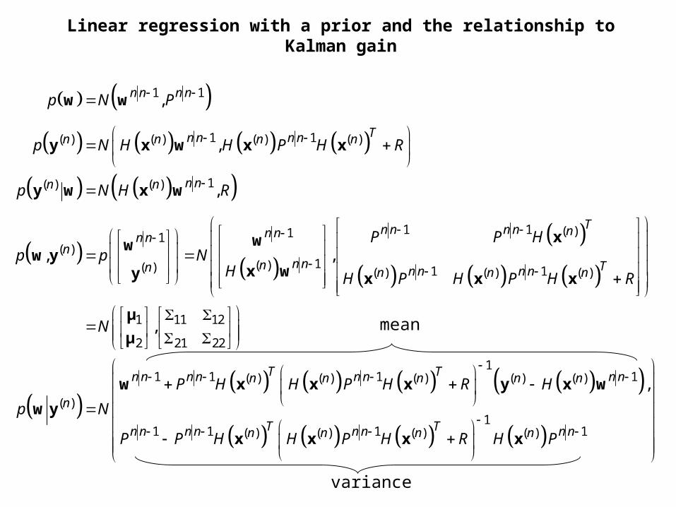
Linear regression with a prior and the relationship to Kalman gain

1 1

1 1( ) ( ) ( ) ( )

1( ) ( )

1 1 ( )11( )

1( )( ) 1 1( ) ( ) ( )

,

,

,

, ,

n n n n

Tn n n nn n n n

n nn n

Tn n n n nn nn nn

n nn Tn n n n nn n n

p N P

p N H H P H R

p N H R

P P Hp p N

H H P H P H R

w w

y x w x x

y w x w

xwww y

x wy x x x

1 11 12

2 21 22

11 1 1 1( ) ( ) ( ) ( ) ( )

( )1

1 1 1 1( ) ( ) ( ) ( )

,

,T Tn n n n n n n nn n n n n

n

T Tn n n n n n n nn n n n

N

P H H P H R H

p N

P P H H P H R H P

μ

μ

w x x x y x w

w y

x x x x

mean

variance

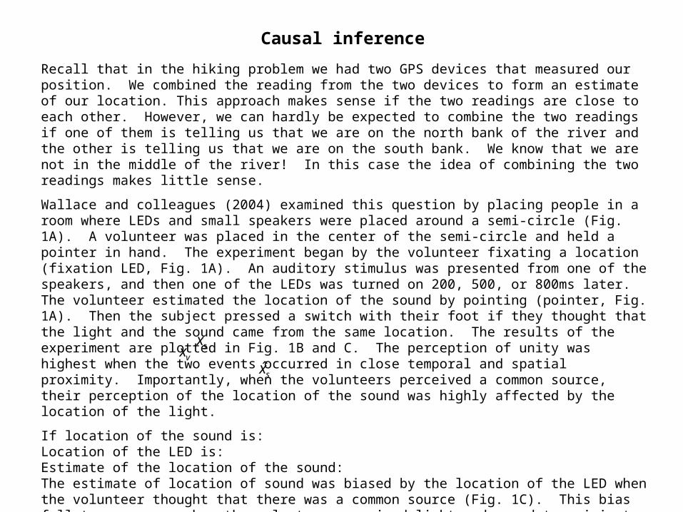
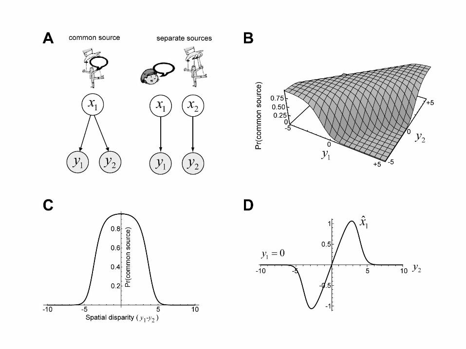
Recall that in the hiking problem we had two GPS devices that measured our position. We combined the reading from the two devices to form an estimate of our location. This approach makes sense if the two readings are close to each other. However, we can hardly be expected to combine the two readings if one of them is telling us that we are on the north bank of the river and the other is telling us that we are on the south bank. We know that we are not in the middle of the river! In this case the idea of combining the two readings makes little sense.

Wallace and colleagues (2004) examined this question by placing people in a room where LEDs and small speakers were placed around a semi-circle (Fig. 1A). A volunteer was placed in the center of the semi-circle and held a pointer in hand. The experiment began by the volunteer fixating a location (fixation LED, Fig. 1A). An auditory stimulus was presented from one of the speakers, and then one of the LEDs was turned on 200, 500, or 800ms later. The volunteer estimated the location of the sound by pointing (pointer, Fig. 1A). Then the subject pressed a switch with their foot if they thought that the light and the sound came from the same location. The results of the experiment are plotted in Fig. 1B and C. The perception of unity was highest when the two events occurred in close temporal and spatial proximity. Importantly, when the volunteers perceived a common source, their perception of the location of the sound was highly affected by the location of the light.

If location of the sound is:Location of the LED is:Estimate of the location of the sound:The estimate of location of sound was biased by the location of the LED when the volunteer thought that there was a common source (Fig. 1C). This bias fell to near zero when the volunteer perceived light and sound to originate from different sources

Causal inference

sxvx

ˆsx

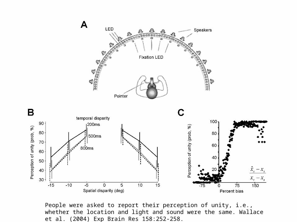
People were asked to report their perception of unity, i.e., whether the location and light and sound were the same. Wallace et al. (2004) Exp Brain Res 158:252-258.

1

2

1 0

0 1 y

x

x

y ε1

2

1 0

1 0 y

x

x

y ε

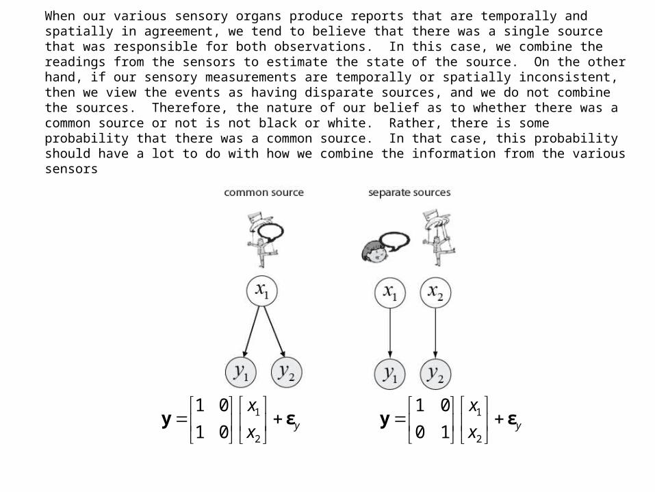
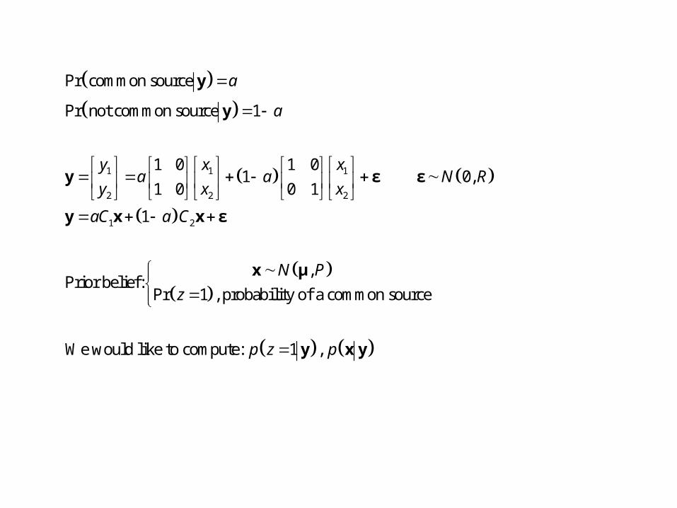
When our various sensory organs produce reports that are temporally and spatially in agreement, we tend to believe that there was a single source that was responsible for both observations. In this case, we combine the readings from the sensors to estimate the state of the source. On the other hand, if our sensory measurements are temporally or spatially inconsistent, then we view the events as having disparate sources, and we do not combine the sources. Therefore, the nature of our belief as to whether there was a common source or not is not black or white. Rather, there is some probability that there was a common source. In that case, this probability should have a lot to do with how we combine the information from the various sensors

1 1 1

2 2 2

1 2

Pr common source

Pr not common source 1

1 0 1 01 0,

1 0 0 1

1

,Prior belief:

Pr 1 , probability of a common source

We woul

a

a

y x xa a N R

y x x

aC a C

N P

z

y

y

y ε ε

y x x ε

x μ

d like to compute: 1 , p z p y x y

1

1 1

2

2 2

1 1 1

2 2 2

1 1 2 2

1 1 2

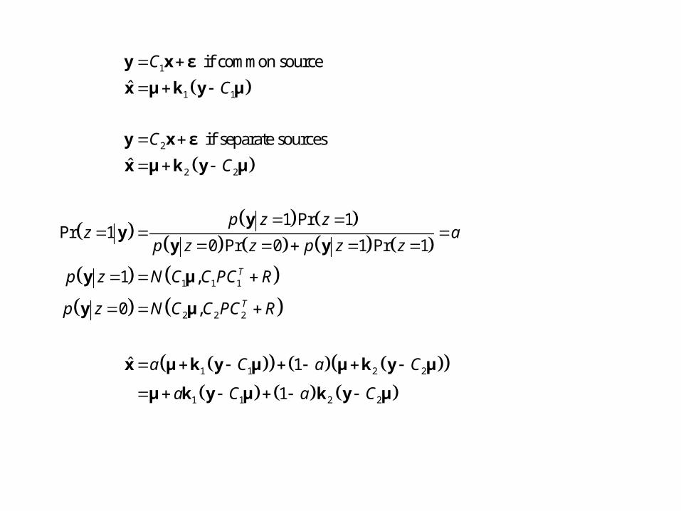
if common source

ˆ

if separate sources

ˆ

1 Pr 1Pr 1

0 Pr 0 1 Pr 1

1 ,

0 ,

ˆ 1

1

T

T

C

C

C

C

p z zz a

p z z p z z

p z N C C PC R

p z N C C PC R

a C a C

a C a

y x ε

x μ k y μ

y x ε

x μ k y μ

yy

y y

y μ

y μ

x μ k y μ μ k y μ

μ k y μ k y 2C μ