55(2006)231-244 Seasonalclimatesummarysouthern hemisphere ... · Introduction Rainwaswelcomedacrossmo stofthecountryduring spring2005,withcentralandeasternAustraliareceiv-ingave ragetoverymuchaboveaverageamounts,in

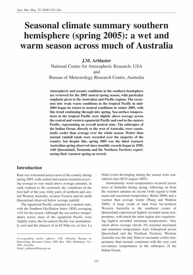
IntroductionRain was welcomed across most of the country duringspring 2005, with central and easternAustralia receiv-ing average to very much above average amounts, instark contrast to the extremely dry conditions of thefirst half of the year. Only parts of northern and cen-tral Western Australia, western Victoria and far northQueensland observed below average rainfall.The equatorial Pacific remained in a neutral state,

with the Southern Oscillation Index (SOI) averaging+4.0 for the season. Although the sea-surface temper-atures across most of the equatorial Pacific wereslightly warm, the far-eastern Pacific was anomalous-ly cool and the chances of an El Niño (or, in fact, La

Niña) event developing during the season were con-sidered slim (SCO August 2005).Anomalously warm temperatures occurred across

most of Australia during spring, following on fromthe warmest autumn on record (with regard to bothmean and maximum temperature; Bettio 2006) and awarmer than average winter (Wang and Watkins2006). A large swath of land from far-northernWestern Australia to the southeast corner ofQueensland experienced highest recorded mean tem-peratures, with much the same region also experienc-ing highest recorded minimum temperatures. Verymuch above average (decile 10) seasonal maximumand minimum temperatures were widespread acrossQueensland and the Northern Territory. WesternAustralia was the only State to encounter cooler tem-peratures than normal, consistent with the very coolsea-surface temperatures in the subtropics of theIndian Ocean.

Aust. Met. Mag. 55 (2006) 231-244

Seasonal climate summary southernhemisphere (spring 2005): a wet andwarm season across much of Australia

J.M. ArblasterNational Center for Atmospheric Research, USA

andBureau of Meteorology Research Centre, Australia

Atmospheric and oceanic conditions in the southern hemisphereare reviewed for the 2005 austral spring season, with particularemphasis given to the Australian and Pacific regions. The excur-sion into weak warm conditions in the tropical Pacific in mid-2004 began its return to neutral conditions in winter 2005, withthis trend continuing through into spring. Sea-surface tempera-tures in the tropical Pacific were slightly above average acrossthe central and western equatorial Pacific and cool in the easternPacific, representing an overall neutral state. The subtropics ofthe Indian Ocean, directly to the west of Australia, were consis-tently cooler than average over the whole season. Wetter thannormal rainfall totals were recorded over the majority of thecountry but despite this, spring 2005 was the third warmestAustralian spring observed since monthly records began in 1950,with Queensland, Tasmania and the Northern Territory experi-encing their warmest spring on record.

Corresponding author address: J.M. Arblaster, Bureau ofMeteorology Research Centre, GPO Box 1289, Melbourne, Vic.3001, Australia.Email: [email protected]

231

With November being the fourteenth successivemonth of above average Australian mean tempera-tures, there was much speculation that 2005 wouldprove to be Australia’s warmest year on record, witha coldest-on-record December being required toavoid such an outcome. The previous warmest yearin Australia was 1998, when the presence of adeclining El Niño helped elevate the global meantemperature. Without such an event appearing in2005, the sustained warmth during the first 11months of the year was clearly influenced by thelong-term trend of increased temperatures, both inAustralia and globally.

DataThe main sources of information used for this sum-mary were the Climate Monitoring Bulletin –Australia (Bureau of Meteorology, Melbourne,Australia) and the Climate Diagnostics Bulletin(Climate Prediction Center, Washington D.C., USA).

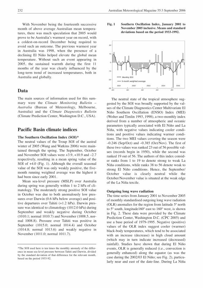
Pacific Basin climate indicesThe Southern Oscillation Index (SOI)*The neutral values of the Troup SOI of the australwinter of 2005 (Wang and Watkins 2006) were main-tained through the spring. The September, Octoberand November SOI values were +3.9, +10.9 and –2.7respectively, resulting in a mean spring value of theSOI of +4.0 (Fig. 1). Although the overall seasonalvalue of the SOI was only weakly positive, the five-month running weighted average was the highest ithad been since early 2001.Mean sea-level pressure (MSLP) over Australia

during spring was generally within 1 to 2 hPa of cli-matology. The moderately strong positive SOI valuein October was due to both anomalously low pres-sures over Darwin (0.6 hPa below average) and posi-tive departures over Tahiti (+1.2 hPa). Darwin pres-sure was identical to climatology (1012.0 hPa) duringSeptember and weakly negative during October(1010.1; normal 1010.7) and November (1008.5, nor-mal 1008.8). Pressure over Tahiti was positive inSeptember (1015.0; normal 1014.4) and October(1014.8; normal 1013.6) and weakly negative inNovember (1011.0; normal 1011.7).

The neutral state of the tropical atmosphere sug-gested by the SOI was broadly supported by the val-ues of the Climate Diagnostics Center Multivariate ElNiño Southern Oscillation (ENSO) Index (MEI)(Wolter and Timlin 1993, 1998), a two-monthly indexderived from a number of atmospheric and oceanicparameters typically associated with El Niño and LaNiña, with negative values indicating cooler condi-tions and positive values indicating warmer condi-tions. The two MEI values covering the season were–0.246 (Sep/Oct) and –0.385 (Oct/Nov). The first ofthese two values was ranked 23 out of 56 possible val-ues (records begin in 1950), while the second wasranked 19 out of 56. The authors of this index consid-er ranks from 1 to 19 to denote strong to weak LaNiña conditions, while ranks 38 to 56 denote weak tostrong El Niño conditions. Hence, the September/October value is clearly neutral while theOctober/November value is situated at the weak edgeof the La Niña tercile.

Outgoing long wave radiationThe time series from January 2001 to November 2005of monthly standardised outgoing long wave radiation(OLR) anomalies for the region from latitude 5º northto 5º south, longitude160º east to 160º west, is shownin Fig. 2. These data were provided by the ClimatePrediction Center, Washington D.C. (CPC 2005) anduse a base period of 1979-1995. Negative (positive)values of the OLR index suggest cooler (warmer)black-body temperatures, which tend to be associatedwith an increase (decrease) in high cloud amount(which may in turn indicate increased (decreased)rainfall). Studies have shown that during El Niñoevents, OLR is generally reduced (i.e., convection isgenerally enhanced) along the equator (as was thecase during the 2002/03 El Niño; see Fig. 2), particu-larly near and east of the date-line. During La Niña

232 Australian Meteorological Magazine 55:3 September 2006

*The SOI used here is ten times the monthly anomaly of the differ-ence in mean sea-level pressure between Tahiti and Darwin, dividedby the standard deviation of that difference for the relevant month,based on the period 1933-92.

Fig. 1 Southern Oscillation Index, January 2001 toNovember 2005 inclusive. Means and standarddeviations based on the period 1933-1992.

| | | | |

events, OLR is often increased (i.e., convection isoften suppressed) over the same region.During the individual months of spring 2005, the

standardised OLR anomaly for this region rose steadi-ly from September (standardised anomaly of +0.1) toOctober (+0.3) with a sharp rise to over one standarddeviation in November (+1.1). The positive values ineach month indicate that convection was generallysuppressed (i.e., cloudiness reduced) in the centralequatorial Pacific during spring 2005, although it wasclose to average throughout the early part of the sea-son. The OLR values for spring 2005 were almost

identical to those of spring 2003 (Watkins 2004),when the equatorial Pacific was also considered to bein a neutral state.Madden-Julian Oscillation (MJO) activity during

spring 2005 was generally weak. There was someindication of convective activity beginning in theIndian Ocean during early September and again inearly November, but both times the convectionpetered out upon entering the Pacific basin.Figure 3 shows the spatial pattern of OLR anom-

alies (relative to a 1979-1998 base period) observedduring the season. There were widespread positiveanomalies (suppressed convection) across the centralequatorial Pacific, and negative (enhanced convec-tion) anomalies over the maritime continent duringSpring 2005. The area of suppressed convectionextended into the far eastern Pacific. These OLR pat-terns resemble those of cool ENSO conditions, inwhich the normal falling (eastern Pacific) and rising(maritime continent) branches of the WalkerCirculation are reinforced. The OLR anomalies dur-ing November 2005 (not shown) were the strongestof the season and configured in a classical La Niña-like pattern, with strongly reduced cloudiness in theequatorial Pacific and a shift of the convection in theSouth Pacific convergence zone to the southwest ofits climatological axis (Vincent 1994). However, asshown earlier, the SOI and multivariate ENSOindices give mixed messages regarding the state ofthe atmosphere during this month, suggesting thatthere was little coupling between the ocean andatmosphere. Across Australia (not shown), OLR val-ues were close to climatology.

Arblaster: Seasonal climate summary spring 2005 233

Fig. 2 Standardised anomaly of monthly outgoinglong wave radiation averaged over 5°N-5°Sand 160°E-160°W, for January 2001 toNovember 2005. Negative (positive) anomaliesindicate enhanced (reduced) convection andrainfall. Base period: 1979-1995. After CPC(2005).

Fig. 3 Anomalies of outgoing long wave radiation for spring 2005 (Wm–2). Base period: 1979-1998.

Ocean patternsSea-surface temperature (SST) patternsSpring 2005 SST anomalies obtained from theNOAA Optimum Interpolation analyses (Reynoldset al. 2002) are shown in Fig. 4. Positive (warm)anomalies (using a base period of 1961-1990) areshown in red shades, and negative (cool) anomaliesin blue shades. Weak warm anomalies were foundacross the western and central equatorial Pacific,consistent with the generally neutral state of theequatorial atmosphere indicated by the weakly posi-tive seasonal average of the SOI. East of about150°W, the equatorial Pacific anomalies were coolerthan average, becoming strongly negative close tothe South American coast with anomalies below–1°C. This pattern of warm anomalies in the centraland west and cool anomalies in the east had firstemerged towards the end of the summer (Beard2005) and was present during autumn (Bettio 2006)and winter (Wang and Watkins 2006). A consistentequatorial Pacific pattern to that shown in Fig. 4 waspresent during each month contributing to spring2005, with the area of cool anomalies expanding fur-ther into the central Pacific during November.The various Niño indices (obtained from the

Bureau of Meteorology’s National Meteorologicaland Oceanographic Centre’s analyses, using a baseperiod of 1961 to 1990) reflect both the weakanomalies and the west-east negative gradient seenin the SST patterns of Fig. 4. The Niño 3.4 index,an area average of SSTs over a region in the cen-tral equatorial Pacific, had a spring 2005 value of+0.06°C, consistent with the neutral value of theSOI and other indicators in reflecting neutral con-

ditions. The individual months were also close toneutral in this region with values of +0.06°C,+0.22°C and –0.09°C for September, October andNovember, respectively. As noted earlier and seenin Fig. 4, the far-eastern Pacific experienced coolanomalies that gradually expanded west during theseason. The Niño 1 and 2 indices, which are locat-ed close to the South American coast, were coolerthan average throughout the season, while theNiño 4 index, in the western Pacific, stayed con-sistently warm.A notable feature of the SST pattern in Fig. 4 is

the region of cooler than average SSTs covering thesouth Indian Ocean, extending from the west coastof Australia to Madagascar and from around 15°Sto 45°S with anomalies of greater than –1°C. SSTsaround the maritime continent were warmer thanaverage. As will be discussed later, the cooling inthe south Indian Ocean, in combination with thesewarm anomalies, has previously been shown tohave a strong positive correlation with rainfallamounts over Australia.Elsewhere anomalies can be seen in the high lati-

tudes of the southwestern Pacific, southern Indian andsouthern Atlantic Ocean basins.Sea-ice formation around Antarctica (not shown)

typically reaches its northernmost extent duringspring, reflecting the minimums in sea-surface tem-peratures that occur in the Southern Ocean at thattime. During spring 2005, increased concentrations ofsea-ice were found in the high southern latitudes ofthe Indian and Western Pacific Oceans and theWeddell and Ross Seas. Only the Bellingshausen andAmundsen Seas, in the longitudes of the southeasternPacific, recorded decreased sea-ice amounts.


Fig. 4 Anomalies of sea-surface temperature for spring 2005 (°C). Base period: 1961-1990. Contour interval is 0.5°C.

Total ice-covered area and extents are calculatedfrom the SSM/I satellite instrument using the NASATeam algorithm (Cavalieri et al. 1984; seehttp://www.nsidc.org). Total sea-ice extent is definedas the area within the 15 per cent concentrationboundary. A consistent time series is available from1987-2005. In total, the Antarctic sea-ice area andextent were both larger during spring 2005 than theirrespective 1987-2005 means. The peak areal extent ofsea-ice for the year (based on monthly data) occurredin September, with a value of 18.81 million km2. Thisamount exceeds the previous maximum extent valueof 18.79 million km2, which was reached duringSeptember 2000. October and November sea-iceextents were also greater than normal, with values of18.41 and 16.52 million km2, respectively.

Subsurface ocean patternsThe Hovmöller diagram for the 20°C isotherm depthanomaly across the equator from January 2001 toNovember 2005 is shown in Fig. 5, based on theBMRC ocean analyses (Smith 1995). The 20°Cisotherm depth is generally situated close to the equa-torial ocean thermocline, the region of greatest tem-perature gradient with depth and the boundarybetween the warm near surface and cold deep oceanwater. Changes in the thermocline depth may act as aprecursor to future changes at the surface.There was very little Kelvin wave activity during

the spring season of 2005, consistent with the lack ofany strong MJO events noted earlier. The equatorialocean thermocline normally tilts down from east towest, with the 20°C isotherm being at shallowerdepths (~50 m) in the eastern Pacific and deeperdepths (~150 m) in the western Pacific warm pool.During all three individual months the thermocline tiltwas somewhat steeper than its climatological statewith a shallowing of the equatorial ocean thermoclinein the eastern Pacific (indicated by negative anom-alies of ~–20 m) and close to normal depths to a slightdeepening in the western Pacific warm pool (indicat-ed by positive anomalies of +10 m).The springtime expansion of cool anomalies into

the central Pacific, which was noted in the descriptionof SSTs, can also be seen in the equatorial Pacifictemperature anomaly profile in Fig. 6. Monthly equa-torial ocean temperature anomalies (from a 1980-1992 climatology) down to 400 metres are shownfrom August to November 2005), with red shadesindicating warm anomalies and blue shades coolanomalies. The general pattern during all months is ofa layer of negative anomalies centred on depths of100-150 m, with these negative anomalies reachingthe surface layers in the eastern Pacific and encasedby positive anomalies above and below at longitudes


Fig. 5 Time-longitude section of the monthly anom-alous depth of the 20°C isotherm at the equa-tor for January 2001 to November 2005. Baseperiod: 1980-1992. Contour interval is 10 m.

Fig. 6 Four-month August 2005 to November 2005sequence of vertical temperature anomalies atthe equator. Base period: 1980-1992. Contourinterval is 0.5°C.

west of the date-line. This pattern was first estab-lished in April 2005 (Wang and Watkins 2006) andwas maintained throughout the winter and spring. Thenegative anomalies became somewhat weaker duringOctober but strengthened again in November, withanomalies of up to –3°C at 140°W in that month.

Atmospheric patternsSurface analysesThe southern hemisphere spring 2005 mean sea-levelpressure pattern, computed from the AustralianBureau of Meteorology’s Global Assimilation andPrediction (GASP) model, is shown in Fig. 7, with thecorresponding anomaly pattern shown in Fig. 8.These anomalies are the difference from a 22-year(1979-2000) climatology obtained from the NationalCenters for Environmental Prediction (NCEP) IIReanalyses (Kanamitsu et al. 2002). The MSLPanalysis has been computed using data from the 0000UTC daily analyses of the GASP model. The MSLPanomaly field is not shown over areas of elevatedtopography (grey shading).The MSLP field for spring showed wave-three

characteristics around Antarctica, with troughs locat-ed around 110°E, 130°W and 0°E. The central lows inthe polar trough itself were located at around 130°E,135°W and 20°E. The MSLP anomaly pattern con-firms to a certain extent this wave-three pattern, withanomalous lows located at 105°E and 135°E. Thethird branch of the pattern was much weaker, howev-er, and the presence of two smaller positive anomalieslocated almost diametrically opposite at around155°E and 60°W complicates this view.MSLPwas below average across most of the equa-

torial Pacific, with positive anomalies only presentwest of about 165°E. In the Australian region, pres-sures were above average across the northern two-thirds of the country (anomalies to +2 hPa), andbelow average across the rest.

Mid-tropospheric analyses and blockingThe 500 hPa geopotential height (an indicator of thesteering of surface synoptic systems) across thesouthern hemisphere is shown in Fig. 9, with anom-alies in the 500 hPa field shown in Fig. 10. The mid-level height anomalies largely reflected the surfacepatterns described above, although in the anomalypattern (Fig. 10) the relative magnitudes of the posi-tive and negative anomalies around Antarctica weremore evenly matched than at the surface.Mid-level heights were above average across most

of Australia (and indeed over most of the tropicalareas to Australia’s north), but negative across south-

ern South Australia and the southern half of WesternAustralia.The time-longitude section of the daily southern-

hemisphere blocking index (BI),

BI = [(u25+v30) – (u40+2u45+u50) + (u55+u60)]/2,

is shown in Fig. 11, with the start of the season at the


Fig. 7 Mean sea-level pressure for spring 2005 (hPa).

Fig. 8 Anomalies of the mean sea level pressure fromthe 1979-2000 National Centers forEnvironmental Prediction reanalysis II clima-tology, for spring 2005 (hPa).

top of the figure. Here, uλ indicates the 500 hPa levelzonal wind component at λ degrees of southern hemi-spheric latitude, under the usual convention that pos-itive (negative) values of uλ correspond to westerly(easterly) winds. This index is a measure of thestrength of the mid-level mid-latitude zonal winds rel-ative to those at higher and lower latitudes at the samelevel. Positive values of the blocking index are gener-ally associated with a split in the mid-latitude wester-ly flow and mid-latitude blocking activity.

Blocking was relatively weak during the season,with BI values exceeding +60 m s–1 only at aroundlongitude 150°W at the very start of the season and ataround 120°E at the start of November. This is con-firmed in the seasonal mean BI (Fig. 12), which indi-cates that blocking was either near average or belowaverage (30°E to 100°E and 170°W to 60°W).

Low-level and upper-level windsSpring 2005 low-level (850 hPa) and upper-level (200hPa) wind anomalies (from the 22-year 1979-2000NCEP II climatology) are shown in Figs 13 and 14respectively. Isotach contours are at 5 m s–1 intervals,and regions where the surface rises above the 850 hPalevel are shaded grey in Fig. 13.


Fig. 9 Mean 500 hPa geopotential heights for spring2005 (gpm).

Fig. 10 Anomalies of the 500 hPa geopotential heightfrom the 1979-2000 National Centers forEnvironmental Prediction reanalysis II clima-tology, for spring 2005 (gpm).

Fig. 11 Spring 2005 daily blocking index: time-longi-tude section (m s–1). Day 1 is 1 September.

Fig. 12 Mean southern hemisphere blocking index forspring 2005 (bold line). The dashed line showsthe corresponding long-term average. Thehorizontal axis shows the degrees east of theGreenwich meridian. (m s–1).

Across the equatorial Pacific, the wind anomalieswere quite weak at both low and upper levels, consis-tent with the neutral ENSO state previouslydescribed. In the far eastern equatorial Pacific, abovethe previously mentioned negative SST anomalies,there was a clockwise cross-equatorial wind anomalypattern in the low levels, although in the upper levels,this feature was shifted somewhat westward.Across Australia, the low-level wind anomalies

were generally northerly in the north, tending north-westerly in the central latitudes. Wind anomalies

across the southwest were consistent with thecyclonic anomaly located to the southwest of thecountry.In the upper levels, an anticyclonic anomaly pat-

tern was evident to the west of the country, centredabove the Indian Ocean at around 20° south. Thisresulted in westerly seasonal wind anomalies inexcess of 5 m s–1 (indicative of an enhanced jetstream) across southwest Western Australia. Anothercontributor to this outcome was the cyclonic anomalypattern to the southwest of the country.


Fig. 13 Spring 850 hPa vector wind anomalies from the 1979-2000 National Centers for Environmental Predictionreanalysis II climatology. Contours of vector magnitude are overlayed. The contour interval is 5 m s–1, with val-ues above 5 m s–1 stippled.

Fig. 14 Spring 2005 200 hPa vector wind anomalies 1979-2000 National Centers for Environmental Prediction reanaly-sis II climatology. Contours of vector magnitude are overlayed. The contour interval is 5 m s–1, with valuesabove 5 m s–1 stippled.

Ozone hole observationsThe austral spring is typically the time of the maximumextent of the Antarctic ozone hole, as well as the timeof lowest annual ozone levels. In the absence of sun-light, the wintertime polar vortex in the lower strato-sphere cools to below –78°C enabling polar stratos-pheric ice clouds to form. Chlorine and bromine com-pounds react in the ice clouds to produce chemicalspecies that, when combined with the incoming UVradiation as the sunlight returns in spring, destroyozone (WMO 1998). As the stratosphere warms inspring (and hence ice clouds can no longer form) thisprocess weakens. Ozone levels then return to near nor-mal by early summer. The compounds that lead to theozone breakdown are largely anthropogenic, but nowappear to be in decline (WMO 1998).Spring ozone totals are shown in Fig. 15. Unlike

previous years the values are taken from the OzoneMonitoring Instrument (OMI), a new instrumentthat effectively continues the ozone record of theTotal Ozone Mapping Spectrometer (TOMS)instruments, which were recently retired. Seehttp://toms.gsfc.nasa.gov for more information.Ozone values are given in Dobson Units and theozone hole is typically taken as the region wherevalues of total column ozone are less than 220Dobson units.The 2005 ozone hole was considered the third

largest on record, reaching a peak of 27 million (M)km2 on 19 September (WMO 2006), much largerthan the previous year’s value of 20M km2 (Bettioand Watkins 2005). Rapid formation of the ozonehole began in early August and by mid-August thetotal area was larger than any previous value record-ed to that time of year, based on TOMS/OMI datafrom 1990-2004. Similar early ozone hole forma-tion occurred in 2003 and 2000, which were the sec-ond largest and largest ozone holes on record,respectively. From mid-August, daily ozone holeareas followed a similar trajectory to 2003, contin-uing to climb for another few weeks. DuringSeptember sustained values of ~24M km2 weremeasured, somewhat lower than during the corre-sponding period in 2003. A minimum total columnozone value of 102 Dobson Units was recorded on1 October 2005, after which the ozone hole began togradually contract. There was a small increase insize during the first week of November, before theozone hole area rapidly declined. By mid-November the ozone hole had almost completelydisappeared. The rapid growth, large size and rapiddecline of the ozone hole were the main features ofthe 2005 season.Consistent with the satellite results, Klekociuk

(2006) found lower than normal ozone amounts in

the ozonesonde measurements over Davis station,Antarctica, during winter and spring 2005. Thiswas despite the fact that a large warming occurredin the lower stratosphere over Davis during thethird week of August, inhibiting the ability of polarstratospheric clouds to chemically process theatmosphere and thus lead to ozone depletion there.However, Klekociuk (2006) note that although thiswarming pushed the polar vortex edge closer toDavis than usual, the station was still located with-in the vortex during September and thus stillobserved the low ozone levels associated with theozone hole.The large size of the 2005 ozone hole, on the back

of the small hole observed in 2004, was a return to thepattern of oscillating years of small and large holesobserved from 1996-2001. This sequence of oscillat-ing ozone hole size had broken down in 2002, whenthe ozone hole split into two separate regions result-ing in a small recorded area in that year, following onfrom a relatively small hole in 2001. The oscillationin ozone hole area has been attributed by some stud-ies (see Baldwin et al. 2001) to the Quasi-BiennialOscillation, a regime that dominates the meteorologi-cal variability of the equatorial stratosphere and hassome interaction with the extratropical and polarregions. This underlines the inherent interannual vari-ability of the meteorology effecting the formation anddestruction of ozone over Antarctica, compoundingefforts to predict the timing of the recovery of theozone hole.


Fig. 15 Total column ozone values from the OzoneMonitoring Instrument (OMI) for spring 2005(Dobson Units).

Australian regionRainfallThe distribution of Australian rainfall totals for spring2005 is shown in Fig. 16, while Fig. 17 shows theassociated decile ranges based on gridded rainfalldata for all springs from 1900 to 2005. Table 1 sum-marises the seasonal rainfall ranks and extremes on anational and State basis.The rainfall distribution (Fig. 16) across Australia

was quite typical for spring, with the highest rainfalltotals recorded in the eastern third of the country andlower amounts registered in the central and westernregions. Rainfall totals above 300 mm occurred acrossthe coastal and mountainous regions of New SouthWales and southern Queensland, in theAustralianAlpsand over most of Tasmania. Mount Read in Tasmaniarecorded the highest total for the season with 906 mm(Table 1). Lowest rainfall totals for the season werefound in the northwest of Western Australia, a regionthat is seasonally dry in spring.As can be seen in Fig. 17, above average rainfall

fell over a significant portion of Australia duringspring, continuing to relieve the dry conditions thatdominated the first half of the year (Shein 2006).Australian area-averaged rainfall for spring was 95mm, 30 per cent above the 1961-1990 normal. Area-averaged rainfall amounts were above average in allStates except for Western Australia, which was nearnormal. Many regions in the Northern Territory,South Australia, New South Wales and Tasmania hadvery much above average (decile 10) rainfall withsome isolated regions recording their highest totals onrecord for spring. It was especially wet in CentralAustralia, with rainfall there being more than doublethe average. In contrast, below average (deciles 2 to3) to very much below average (decile 1) rainfalloccurred in central and northwestern WesternAustralia. Far north Queensland and western Victoriaalso recorded below average rainfall during spring2005. Rainfall was near average (deciles 4 to 7) overmost of Queensland.These rainfall decile patterns were quite stable

during the individual months of to the season (notshown). October was especially wet in CentralAustralia, giving the Northern Territory and SouthAustralia their fifth and seventh highest Octobertotals of the past 106 years, respectively. SouthwestWestern Australia also had good rains in October,with several towns there recording more than 50 mmor more above their October averages. Good falls dur-ing October gave southwestern Victoria some respitefrom successive years of below average rainfall, butNovember totals were again below average. Rainfallhas been extremely low by historical standards across

much of southern Victoria in the period since October1996. The nine years to September 2005 has seenlowest on record totals in southwest Victoria (extend-ing into southeast South Australia) and an area imme-diately to the east of Melbourne. Rainfall along theQueensland coast was below average in Septemberand November and above average to very muchabove average (decile 10) during October, while theQueensland interior was close to average during allthree months. Tasmania and the eastern half of NewSouth Wales recorded consistently above averagerainfall throughout the spring, while the northwest ofWestern Australia was consistently below averagewith very much below average (decile 1) rainfall dur-ing November.


Fig. 16 Rainfall totals over Australia for spring 2005(mm).

Fig. 17 Spring 2005 rainfall deciles for Australia:decile range based on grid-point values overthe spring periods from 1900 to 2005.

TemperaturesThe spring mean maximum and minimum tempera-ture anomalies, calculated with respect to the 1961-1990 reference period, are shown in Figs 18 and 19respectively. These analyses use the entire tempera-ture observation network. A high quality subset ofthe network is used to calculate the spatial averagesand rankings shown in Tables 2 and 3, as well as thetemperature deciles referred to below. The area-averaged temperature time series cover the period1950 to 2005.Averaged across Australia, spring 2005 was

ranked the third warmest spring since records beganin 1950. The all-Australian mean temperature anom-aly for spring was +0.98°C (behind +1.13°C in 2002and +1.00°C in 1980), with both overnight minimumtemperatures (+1.12°C) and daytime maximum tem-peratures (+0.83°C) contributing to the overallwarmth. All States and territories experienced aboveaverage maximum and minimum temperatures, withQueensland, Tasmania and the Northern Territory allexperiencing their warmest springs on record.Following on from the warmest autumn on record(Bettio 2006) and an anomalously warm winter(Wang and Watkins 2006), the continued warmth dur-ing spring, without the presence of any significantactivity in the Pacific and with the usually coolingeffects of above average rainfall, puts these latestresults in quite a remarkable context. There was muchspeculation during November with regards to the con-sistent warmth throughout the year, with projectionsthat 2005 would prove to be Australia’s warmest yearon record unless a coldest on record December even-

tuated. With respect to area-averaged maximum tem-peratures, Queensland, Tasmania and the NorthernTerritory recorded their third warmest springs onrecord, while with respect to area-averaged minimumtemperatures, the Northern Territory recorded itswarmest spring, Queensland and Tasmania their sec-ond warmest spring, and New South Wales and SouthAustralia their third warmest spring.As can be seen in Figs 18 and 19, positive temper-

ature anomalies covered most of the country duringspring. A large swath of the country from northwest-ern Western Australia to southeast Queensland expe-rienced very large maximum and minimum tempera-ture anomalies in spring. Mean temperature anom-alies were the highest on record in this region, withminimum temperature anomalies also being higheston record over much the same region. The regionoverlaps to a considerable extent the area of verymuch above average rainfall (decile 10) seen in Fig.17, indicating that the warm night-time temperatureswere possibly associated with increased cloud coverat night there; a situation which would act to trap theoutgoing long wave radiation. By the same argumentone might have expected maximum temperatures tobe cooler than average, with the rain-filled cloudsreflecting the incoming solar radiation and alsoincreasing surface latent heat fluxes, but Fig. 19 clear-ly shows this not to be the case. This is consistent withthe results of Nicholls et al. (1996), who showed thatthe relationship between maximum temperature andrainfall has changed in recent years, with maximumtemperatures tending to be higher, relative to rainfall,than was previously the case.


Table 1. Summary of the seasonal rainfall ranks and extremes on a national and State basis.

Highest seasonal Lowest seasonal Highest 24-hour Area-averaged Rank oftotal (mm) total (mm) fall (mm) rainfall (aar) aar*

(mm)

Australia 903 at Mount Read Zero at several WA 220 at German Town (TAS) 95 90(TAS) locations on 22 October

WA 436 at Willowdale Zero at several 64 at Allan Rocks 40 70locations on 17 October

NT 442 at Howard Springs 35 at Tobermorey 164 at Darwin River Dam 121 97on 24 October

SA 519 at Piccadilly 20 at Moomba 118 at Uraidla on 8 November 96 100QLD 541 at Caboolture 8 at Wyora 154 at Roundstone Creek 90 69

on 16 OctoberNSW 681 at Leigh 10 at Monolon 187 at Buckenbowra 180 91

on 31 OctoberVIC 640 at Rocky Valley 89 at Pella 91 at Cabbage Tree Creek 191 66

on 29 NovemberTAS 903 at Mount Read 164 at Clyde River 220 at German Town 402 98

on 22 October

* The rank goes from 1 (lowest) to 106 (highest) and is calculated on the years 1900 to 2005 inclusive.

In contrast to the rest of the country, the south-western third of Western Australia recorded belowaverage (deciles 2 to 3) temperature anomalies in boththe maximum and minimum temperature fields.Departures from normal were not as extreme in NewSouth Wales, but anomalously warm temperatureswere also recorded across most of that State.Temperatures were also very much above average(decile 10) in the southern regions of Victoria andacross Tasmania. Relatively few regions experiencedaverage (deciles 4 to 7) conditions, with the interior ofWestern Australia, parts of western Victoria and NewSouth Wales and a small region in northernQueensland being the exceptions.For the individual months (not shown), largest

minimum temperature departures occurred inSeptember and October, with anomalies of +3°Cencompassing the southern three-quarters of theNorthern Territory and the Darling Downs area ofQueensland. The Northern Territory also recordedsimilarly large maximum temperature anomalies inSeptember, with departures weakening to +2°C inOctober. Most of Queensland was warmer than aver-age by at least +2°C during October. Cool anomaliesof up to –3°C occurred in southwestern WesternAustralia during October.In area-averaged terms, Australian mean tempera-

tures during September, October and November wereall well above their 1961-1990 norms, with anomaliesof +1.13, +1.08, +0.72°C, respectively. A number ofhighest on record minimum temperatures were set dur-ing the individual months, with the Northern Territoryrecording its highest September minimum temperature(anomaly of +2.59°C; based on records since 1950),and Queensland and Tasmania recording their highest

October minimum temperatures (anomalies of +2.37and +1.75°C, respectively). Maximum temperatureanomalies were also strongly positive in all months, forall States except WesternAustralia, which was the onlyState during the season to record a negative maximumtemperature anomaly (during October). Mean tempera-tures over New South Wales and Victoria were close toaverage during September but became warm again dur-ing October and November.The west to east gradient in the spring tempera-

ture patterns over Australia, with cool anomalies inthe west and warm anomalies in the eastern two-thirds, occurred in all three months that contributedto the season, inferring a strong influence from a sta-ble pattern of sea-surface temperatures. As notedearlier, SSTs directly to the west of WesternAustralia were anomalously cool, resulting inonshore winds bringing cooler than normal air to thewest. Although a mixed signal was found in theENSO indices, the SSTs directly to the north ofAustralia were anomalously warm for this time ofyear. Drosdowsky (1993), following on from thework of Nicholls (1989), showed that a pattern ofwarm SSTs to the north of Australia in conjunctionwith cool SSTs in the central Indian Ocean, washighly correlated with anomalously wet conditionsover Australia. The climate patterns of spring 2005are consistent with their results.

AcknowledgmentsThe author would like to acknowledge the valuableinput of Dr Robert Fawcett to this manuscript. DrsAndrew Watkins and Grant Beard also gave useful


Fig. 18 Spring 2005 maximum temperature anomaliesfor Australia based on a 1961-90 mean (°C).

Fig. 19 Spring 2005 minimum temperature anomaliesfor Australia based on a 1961-90 mean (°C).

comments on early drafts. A portion of this study wassupported by the Office of Biological andEnvironmental Research, US Department of Energy,

as part of its Climate Change Prediction Program. TheNational Center for Atmospheric Research is spon-sored by the National Science Foundation.


Table 2. Summary of the seasonal maximum temperature ranks and extremes on a national and State basis.

Highest Lowest Highest Lowest Anomaly of Rank ofseasonal seasonal daily daily area-averaged aam*

mean (°C) mean (°C) recording (°C) recording (°C) mean (°C) (aam)

Australia 40.5 at Fitzroy 7.3 at Mt Hotham 46.0 at Marble Bar –2.8 at Thredbo Top +0.83 48Crossing (WA) (VIC) (WA) on Station (NSW) on

25 November 12 SeptemberWA 40.5 at Fitzroy 17.1 at Shannon 46.0 at Marble Bar 9.7 at Mount Barker +0.12 29

Crossing on 25 November on 27 SeptemberNT 38.4 at Rabbit Flat 30.7 at McCluer 43.5 at Rabbit Flat 18.0 at Kulgera +1.29 54

Island on 26 October on 11 SeptemberSA 31.5 at Moomba 14.9 at Mount Lofty 44.0 at Moomba 5.3 at Mount Lofty +0.89 43

on 9 November on 11 SeptemberQLD 38.0 at Julia Creek 23.0 at Applethorpe 45.5 at Birdsville 11.0 at Applethorpe +1.49 54

on 9 November on 17 SeptemberNSW 30.4 at Wanaaring 7.9 at Thredbo Top 42.8 at Tibooburra –2.8 at Thredbo Top +0.78 43

Station on 9 November Station on 12 SeptemberVIC 23.9 at Mildura 7.3 at Mt Hotham 35.9 at Mildura on –2.6 at Mt Hotham +0.75 45

25 November on 12 SeptemberTAS 18.8 at Bushy Park 8.2 at Mount 30.3 at Scotts Peak –0.9 at Mount +0.82 52

Wellington Dam on 7 November Wellington on12 September

* The temperature ranks go from 1 (lowest) to 56 (highest) and are calculated on the years 1950 to 2005 inclusive.

Table 3. Summary of the seasonal minimum temperature ranks and extremes on a national and State basis.

Highest Lowest Highest Lowest Anomaly of Rank ofseasonal seasonal daily daily area-averaged aam*

mean (°C) mean (°C) recording (°C) recording (°C) mean (°C) (aam)

Australia 27.1 at Troughton 0.5 at Thredbo Top 32.2 at Wittenoom –11.0 at Charlotte +1.12 55Island (WA) Station (NSW) (WA) on 25 Pass (NSW) on

November 1 SeptemberWA 27.1 at Troughton 5.7 at Wandering 32.2 at Wittenoom –3.2 at Southern Cross +0.38 39

Island on 25 November on 10 SeptemberNT 26.3 at McCluer 15.9 at Yulara 29.7 at Ngukurr 2.8 at Yulara on +1.67 56

Island on 24 October and 16 Septemberat Rabbit Flat on31 October

SA 16.6 at Moomba 6.6 at Munkora 28.4 at Moomba –1.2 at Yongala on +1.28 54on 29 October 18 September

QLD 25.3 at Sweers 10.2 at Applethorpe 30.3 at Julia Creek –1.0 at Oakey +1.78 55Island on 7 November on 18 September

NSW 17.4 at Byron Bay 0.5 at Thredbo Top 29.2 at Ivanhoe –11.0 at Charlotte Pass +1.06 54Station on 3 November on 1 September

VIC 12.0 at Point Hicks 1.1 at Mt Hotham 24.7 at Avalon on –8.2 at Mt Hotham +0.60 513 November on 1 September

TAS 11.0 at Swan Island 1.5 at Liawenee 20.4 at Flinders –7.6 at Liawenee +1.09 55Island on on 26 September3 November

* The temperature ranks go from 1 (lowest) to 56 (highest) and are calculated on the years 1950 to 2005 inclusive.

ReferencesBaldwin, M.P., Gray, L.J., Dunkerton, T.J., Hamilton, K., Haynes,

P.H., Randel, W.J., Holton, J.R., Alexander, M.J., Hirota, I.,Horinouchi, T., Jones, D.B.A., Kinnersley, J.S., Marquardt, C.,Sato, K. and Takahashi, M. 2001. The Quasi-BiennialOscillation. Rev. Geophys., 39, 179-229.

Beard, G. 2005. Seasonal climate summary southern hemisphere(summer 2004/2005): a neutral ENSO situation with a coolingPacific. Hot and dry over the western half of Australia. Aust. Met.Mag., 54, 347-57.

Bettio, L. 2006. Seasonal climate summary southern hemisphere(autumn 2005): an exceptionally warm and dry autumn acrossAustralia. Aust. Met. Mag., 55, 71-84.

Bettio, L. and Watkins, A.B. 2005. Seasonal climate summary south-ern hemisphere (spring 2004): neutral conditions remain in thetropical Pacific and a warm spring across Australia. Aust. Met.Mag., 54, 225-39.

Cavalieri, D.J., Gloersen, P. and Campbell, W.J. 1984. Determinationof sea ice parameters with the NIMBUS-7 SMMR. J. Geophys.Res., 89(D4), 5355-69.

Climate Prediction Center 2005. Climate Diagnostics Bulletin,September 2005, October 2005, November 2005. US Departmentof Commerce, National Oceanic and AtmosphericAdministration, Washington D.C.

Drosdowsky, W. 1993. An analysis of Australian seasonal rainfallanomalies: 1950-1987. II: Temporal variability and teleconnec-tion patterns. Int. J. Climatol., 13, 111-49.

Kanamitsu, M., Ebisuzaki, W., Woollen, J., Yang, S.-K., Hnilo, J.J.,Fiorino, M. and Potter, G.L. 2002. NCEP-DOE AMIP-II Re-analysis (R-2). Bull. Am. Met. Soc., 83, 1631-43.

Klekociuk, A.R. 2006. Ozone and temperature above Davis,Antarctica, during the austral winter and spring of 2005. BMRCRes. Lett., 4, 11-15.

Nicholls, N. 1989. Sea surface temperatures and Australian WinterRainfall. Jnl climate, 2, 965-73.

Nicholls, N., Lavery, B., Fredericksen, C., Drosdowsky, W. andTorok, S. 1996. Recent apparent changes in relationshipsbetween the El Niño-Southern Oscillation and Australian rainfalland temperature. Geophys. Res. Lett., 23, 3357-60.

National Climate Centre 2005. Seasonal Climate Outlook for Spring2005 (September to November). Bur. Met., Australia.

Reynolds, R.W., Rayner, N.A., Smith, T.M., Stokes, D.C. and Wang,W. 2002. An improved in situ and satellite SST analysis for cli-mate. Jnl climate, 15, 1609-25.

Shein, K.A. 2006. State of the Climate in 2005. Bull. Am. Met. Soc.,87, s1-s102.

Smith, N. 1995. The BMRC ocean thermal analysis system. Aust.Met. Mag., 44, 93-110.

Vincent D.G. 1994. The South Pacific Convergence Zone (SPCZ): Areview. Mon. Weath. Rev., 122, 1949-70.

Wang, X. and Watkins, A.B. 2006. Seasonal climate summary south-ern hemisphere (winter 2005): neutral conditions in the tropicalPacific and a wet and warm winter across Australia. Aust. Met.Mag., 55, 149-60.

Watkins, A.B. 2004. Seasonal climate summary southern hemisphere(spring 2003): neutral conditions remain in the tropical Pacific,but dry conditions dominate northeast Australia. Aust. Met. Mag.,53, 217-31.

Wolter, K. and Timlin, M.S. 1993. Monitoring ENSO in COADSwith a seasonally adjusted principal component index. Proc. ofthe 17th Climate Diagnostics Workshop, Norman, OK, NOAA/NMC/CAC, NSSL, Oklahoma Clim. Survey, CIMMS and theSchool of Meteorology, Univ. of Oklahoma, 52-7.

Wolter, K. and Timlin, M.S. 1998. Measuring the strength of ENSO- how does 1997/98 rank? Weather, 53, 315-24.

WMO 1998. ‘Record Ozone Depletion in the Antarctic’. WMO PressRelease No. 619. I October 1998. http://www.wmo.ch/web/Press/Press619.html

WMO 2006. Antarctic ozone bulletin winter/spring summary,8/2005, (World Meteorological Organization),(http://www.wmo.ch/web/arep/05/bulletin-8-2005.pdf)

AppendixThe main sources for data used in this review were:• National Climate Centre, Climate Monitoring

Bulletin - Australia. Obtainable from the NationalClimate Centre, Bureau of Meteorology, GPO Box1289, Melbourne, Vic. 3001, Australia.

• The Bureau of Meteorology’s Monthly SignificantWeather Summaries. Obtainable fromhttp://www.bom.gov.au/inside/services_policy/public/sigwxsum/sigwmenu.shtml

• Climate Prediction Center, Climate DiagnosticsBulletin. Obtainable from the Climate PredictionCenter, National Weather Service, WashingtonD.C., USA, 20233.


Documents

55(2006)231-244 Seasonalclimatesummarysouthern hemisphere ... · Introduction Rainwaswelcomedacrossmo stofthecountryduring spring2005,withcentralandeasternAustraliareceiv-ingave ragetoverymuchaboveaverageamounts,in