Embed Size (px)
Citation preview

5.3. APPLICATIONS OF POLYNOMIALS 321
5.3 Applications of Polynomials
In this section we investigate real-world applications of polynomial functions.
You Try It!
EXAMPLE 1. The average price of a gallon of gas at the beginning of eachmonth for the period starting in November 2010 and ending in May 2011 aregiven in the margin. The data is plotted in Figure 5.18 and fitted with thefollowing third degree polynomial, where t is the number of months that havepassed since October of 2010.
p(t) = −0.0080556t3 + 0.11881t2 − 0.30671t+ 3.36 (5.2)
Use the graph and then the polynomial to estimate the price of a gallon of gasin California in February 2011.
Month PriceNov. 3.14Dec. 3.21Jan 3.31Mar. 3.87Apr. 4.06May 4.26
3
3.10
3.20
3.30
3.40
3.50
3.60
3.70
3.80
3.90
4
4.10
4.20
4.30
4.40
4.50
0 1 2 3 4 5 6 7 8t
p(t)
Oct Nov Dec Jan Feb Mar Apr May Jun
Figure 5.18: Fitting gas price versus month with a cubic polynomial.
Solution: Locate February (t = 4) on the horizontal axis. From there, drawa vertical arrow up to the graph, and from that point of intersection, a secondhorizontal arrow over to the vertical axis (see Figure 5.19). It would appearthat the price per gallon in February was approximately $3.51.

322 CHAPTER 5. POLYNOMIAL FUNCTIONS
3
3.10
3.20
3.30
3.40
3.50
3.60
3.70
3.80
3.90
4
4.10
4.20
4.30
4.40
4.50
0 1 2 3 4 5 6 7 8t
p(t)
Oct Nov Dec Jan Feb Mar Apr May Jun
Figure 5.19: Approximating price of gas during February.
Next, we’ll use the fitted third degree polynomial to approximate the priceper gallon for the month of February, 2011. Start with the function defined byequation 5.2 and substitute 4 for t.
p(t) = −0.0080556t3 + 0.11881t2 − 0.30671t+ 3.36
p(4) = −0.0080556(4)3 + 0.11881(4)2 − 0.30671(4) + 3.36
Use the calculator to evaluate p(4) (see Figure 5.20). Rounding to the nearest
Figure 5.20: Evaluating p(4).
penny, the price in February was $3.52 per gallon.
�

5.3. APPLICATIONS OF POLYNOMIALS 323
You Try It!
EXAMPLE 2. If a projectile is fired into the air, its height above ground at If a projectile is launchedwith an initial velocity of 60meters per second from arooftop 12 meters aboveground level, at what timewill the projectile first reacha height of 150 meters?
any time is given by the formula
y = y0 + v0t−1
2gt2, (5.3)
where
y = height above ground at time t,
y0 = initial height above ground at time t = 0,
v0 = initial velocity at time t = 0,
g = acceleration due to gravity,
t = time passed since projectile’s firing.
If a projectile is launched with an initial velocity of 100 meters per second(100m/s) from a rooftop 8 meters (8m) above ground level, at what time willthe projectile first reach a height of 400 meters (400m)? Note: Near the earth’ssurface, the acceleration due to gravity is approximately 9.8 meters per secondper second (9.8 (m/s)/s or 9.8m/s2).
Solution: We’re given the initial height is y0 = 8m, the initial velocity isv0 = 100m/s, and the acceleration due to gravity is g = 9.8m/s2. Substitutethese values in equation 5.3, then simplify to produce the following result:
y = y0 + v0t−1
2gt2
y = 8 + 100t−1
2(9.8)t2
y = 8 + 100t− 4.9t2
Enter y = 8 + 100t− 4.9t2 as Y1=8+100*X-4.9*X∧2 in the Y= menu (see In this example, the horizon-tal axis is actually the t-axis.So when we set Xmin andXmax, we’re actually settingbounds on the t-axis.
the first image in Figure 5.21). After some experimentation, we settled on theWINDOW parameters shown in the second image in Figure 5.21. Push theGRAPH button to produce the graph of y = 8 + 100t − 4.9t2 shown in thethird image Figure 5.21.
Figure 5.21: Sketching the graph of y = 8 + 100t− 4.9t2.

324 CHAPTER 5. POLYNOMIAL FUNCTIONS
To find when the projectile reaches a height of 400 meters (400m), substi-tute 400 for y to obtain:
400 = 8 + 100t− 4.9t2 (5.4)
Enter the left-hand side of Equation 5.4 into Y2 in the Y= menu, as shown inthe first image in Figure 5.22. Push the GRAPH button to produce the resultshown in the second image in Figure 5.22. Note that there are two points ofintersection, which makes sense as the projectile hits 400 meters on the wayup and 400 meters on the way down.
Figure 5.22: Determining when the object first reaches 400 meters.
.
To find the first point of intersection, select 5:intersect from the CALCmenu. Press ENTER in response to “First curve,” then press ENTER againin response to “Second curve.” For your guess, use the arrow keys to movethe cursor closer to the first point of intersection than the second. At thispoint, press ENTER in response to “Guess.” The result is shown in the thirdimage in Figure 5.22. The projectile first reaches a height of 400 meters atapproximately 5.2925359 seconds after launch.The parabola shown in
Figure 5.23 is not the actualflight path of the projectile.The graph only predicts theheight of the projectile as afunction of time.
t(s)
y(m)
25−100
600
5.2925359
y = 8 + 100t− 4.9t2
y = 400
Figure 5.23: Reporting your graphical solution on your homework.
Reporting the solution on your homework: Duplicate the image in yourcalculator’s viewing window on your homework page. Use a ruler to draw alllines, but freehand any curves.
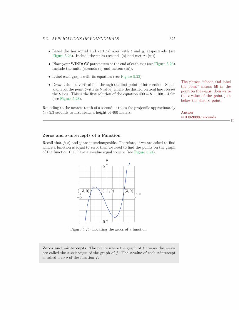
5.3. APPLICATIONS OF POLYNOMIALS 325
• Label the horizontal and vertical axes with t and y, respectively (seeFigure 5.23). Include the units (seconds (s) and meters (m)).
• Place yourWINDOW parameters at the end of each axis (see Figure 5.23).Include the units (seconds (s) and meters (m)).
• Label each graph with its equation (see Figure 5.23).
• Draw a dashed vertical line through the first point of intersection. ShadeThe phrase “shade and labelthe point” means fill in thepoint on the t-axis, then writethe t-value of the point justbelow the shaded point.
and label the point (with its t-value) where the dashed vertical line crossesthe t-axis. This is the first solution of the equation 400 = 8+100t−4.9t2
(see Figure 5.23).
Rounding to the nearest tenth of a second, it takes the projectile approximatelyt ≈ 5.3 seconds to first reach a height of 400 meters. Answer:
≈ 3.0693987 seconds�
Zeros and x-intercepts of a Function
Recall that f(x) and y are interchangeable. Therefore, if we are asked to findwhere a function is equal to zero, then we need to find the points on the graphof the function that have a y-value equal to zero (see Figure 5.24).
−5 5
−5
5
x
y
(−3, 0) (−1, 0) (3, 0)
f
Figure 5.24: Locating the zeros of a function.
Zeros and x-intercepts. The points where the graph of f crosses the x-axisare called the x-intercepts of the graph of f . The x-value of each x-interceptis called a zero of the function f .
326 CHAPTER 5. POLYNOMIAL FUNCTIONS
The graph of f crosses the x-axis in Figure 5.24 at (−3, 0), (−1, 0), and(3, 0). Therefore:
• The x-intercepts of f are: (−3, 0), (−1, 0), and (3, 0)
• The zeros of f are: −3, −1, and 3
Key idea. A function is zero where its graph crosses the x-axis.
You Try It!
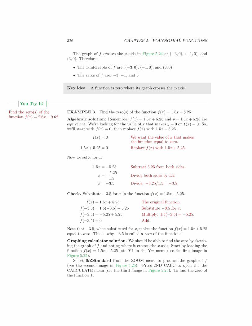
EXAMPLE 3. Find the zero(s) of the function f(x) = 1.5x+ 5.25.Find the zero(s) of thefunction f(x) = 2.6x− 9.62.
Algebraic solution: Remember, f(x) = 1.5x+ 5.25 and y = 1.5x+ 5.25 areequivalent. We’re looking for the value of x that makes y = 0 or f(x) = 0. So,we’ll start with f(x) = 0, then replace f(x) with 1.5x+ 5.25.
f(x) = 0 We want the value of x that makesthe function equal to zero.
1.5x+ 5.25 = 0 Replace f(x) with 1.5x+ 5.25.
Now we solve for x.
1.5x = −5.25 Subtract 5.25 from both sides.
x =−5.25
1.5Divide both sides by 1.5.
x = −3.5 Divide: −5.25/1.5 = −3.5
Check. Substitute −3.5 for x in the function f(x) = 1.5x+ 5.25.
f(x) = 1.5x+ 5.25 The original function.
f(−3.5) = 1.5(−3.5) + 5.25 Substitute −3.5 for x.
f(−3.5) = −5.25 + 5.25 Multiply: 1.5(−3.5) = −5.25.
f(−3.5) = 0 Add.
Note that −3.5, when substituted for x, makes the function f(x) = 1.5x+5.25equal to zero. This is why −3.5 is called a zero of the function.
Graphing calculator solution. We should be able to find the zero by sketch-ing the graph of f and noting where it crosses the x-axis. Start by loading thefunction f(x) = 1.5x + 5.25 into Y1 in the Y= menu (see the first image inFigure 5.25).
Select 6:ZStandard from the ZOOM menu to produce the graph of f(see the second image in Figure 5.25). Press 2ND CALC to open the theCALCULATE menu (see the third image in Figure 5.25). To find the zero ofthe function f :
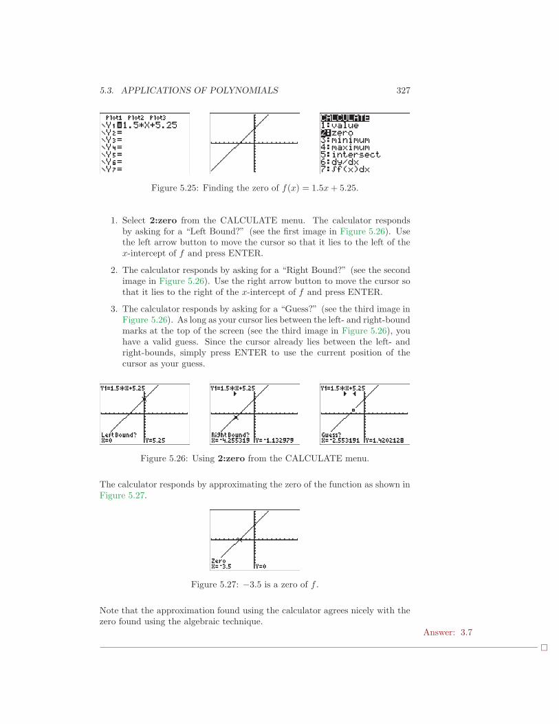
5.3. APPLICATIONS OF POLYNOMIALS 327
Figure 5.25: Finding the zero of f(x) = 1.5x+ 5.25.
1. Select 2:zero from the CALCULATE menu. The calculator respondsby asking for a “Left Bound?” (see the first image in Figure 5.26). Usethe left arrow button to move the cursor so that it lies to the left of thex-intercept of f and press ENTER.
2. The calculator responds by asking for a “Right Bound?” (see the secondimage in Figure 5.26). Use the right arrow button to move the cursor sothat it lies to the right of the x-intercept of f and press ENTER.
3. The calculator responds by asking for a “Guess?” (see the third image inFigure 5.26). As long as your cursor lies between the left- and right-boundmarks at the top of the screen (see the third image in Figure 5.26), youhave a valid guess. Since the cursor already lies between the left- andright-bounds, simply press ENTER to use the current position of thecursor as your guess.
Figure 5.26: Using 2:zero from the CALCULATE menu.
The calculator responds by approximating the zero of the function as shown inFigure 5.27.
Figure 5.27: −3.5 is a zero of f .
Note that the approximation found using the calculator agrees nicely with thezero found using the algebraic technique.
Answer: 3.7
�
328 CHAPTER 5. POLYNOMIAL FUNCTIONS
You Try It!
EXAMPLE 4. How long will it take the projectile in Example 2 to returnIf a projectile is launchedwith an initial velocity of 60meters per second from arooftop 12 meters aboveground level, at what timewill the projectile return toground level?
to ground level?
Solution: In Example 2, the height of the projectile above the ground as afunction of time is given by the equation
y = 8 + 100t− 4.9t2.
When the projectile returns to the ground, its height above ground will bezero meters. To find the time that this happens, substitute y = 0 in the lastequation and solve for t.
0 = 8 + 100t− 4.9t2
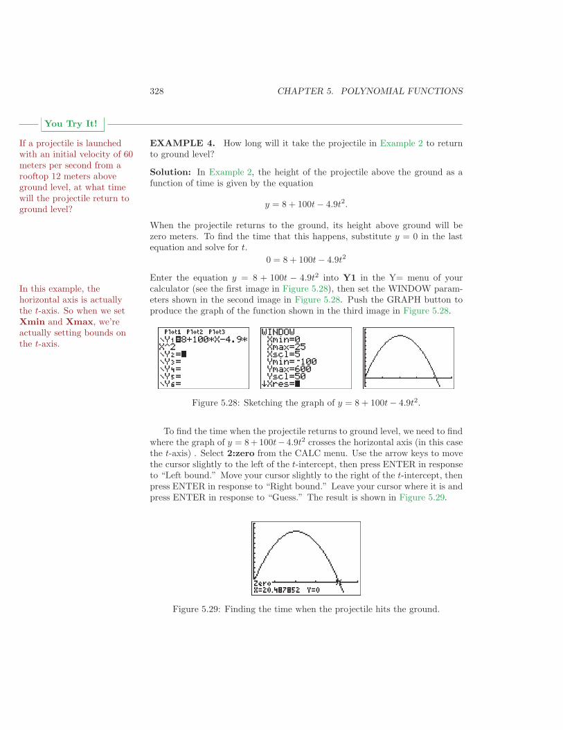
Enter the equation y = 8 + 100t − 4.9t2 into Y1 in the Y= menu of yourcalculator (see the first image in Figure 5.28), then set the WINDOW param-In this example, the
horizontal axis is actuallythe t-axis. So when we setXmin and Xmax, we’reactually setting bounds onthe t-axis.
eters shown in the second image in Figure 5.28. Push the GRAPH button toproduce the graph of the function shown in the third image in Figure 5.28.
Figure 5.28: Sketching the graph of y = 8 + 100t− 4.9t2.
To find the time when the projectile returns to ground level, we need to findwhere the graph of y = 8+100t− 4.9t2 crosses the horizontal axis (in this casethe t-axis) . Select 2:zero from the CALC menu. Use the arrow keys to movethe cursor slightly to the left of the t-intercept, then press ENTER in responseto “Left bound.” Move your cursor slightly to the right of the t-intercept, thenpress ENTER in response to “Right bound.” Leave your cursor where it is andpress ENTER in response to “Guess.” The result is shown in Figure 5.29.
Figure 5.29: Finding the time when the projectile hits the ground.

5.3. APPLICATIONS OF POLYNOMIALS 329
• Label the horizontal and vertical axes with t and y, respectively (seeFigure 5.30). Include the units (seconds (s) and meters (m)).
• Place yourWINDOW parameters at the end of each axis (see Figure 5.30).
• Label the graph with its equation (see Figure 5.30).
• Draw a dashed vertical line through the t-intercept. Shade and label thet-value of the point where the dashed vertical line crosses the t-axis. Thisis the solution of the equation 0 = 8 + 100t− 4.9t2 (see Figure 5.30).
t(s)
y(m)
25−100
600
20.487852
y = 8 + 100t− 4.9t2
Figure 5.30: Reporting your graphical solution on your homework.
Rounding to the nearest tenth of a second, it takes the projectile approximatelyt ≈ 20.5 seconds to hit the ground. Answer:
≈ 12.441734 seconds�
330 CHAPTER 5. POLYNOMIAL FUNCTIONS
§ § § Exercises § § §
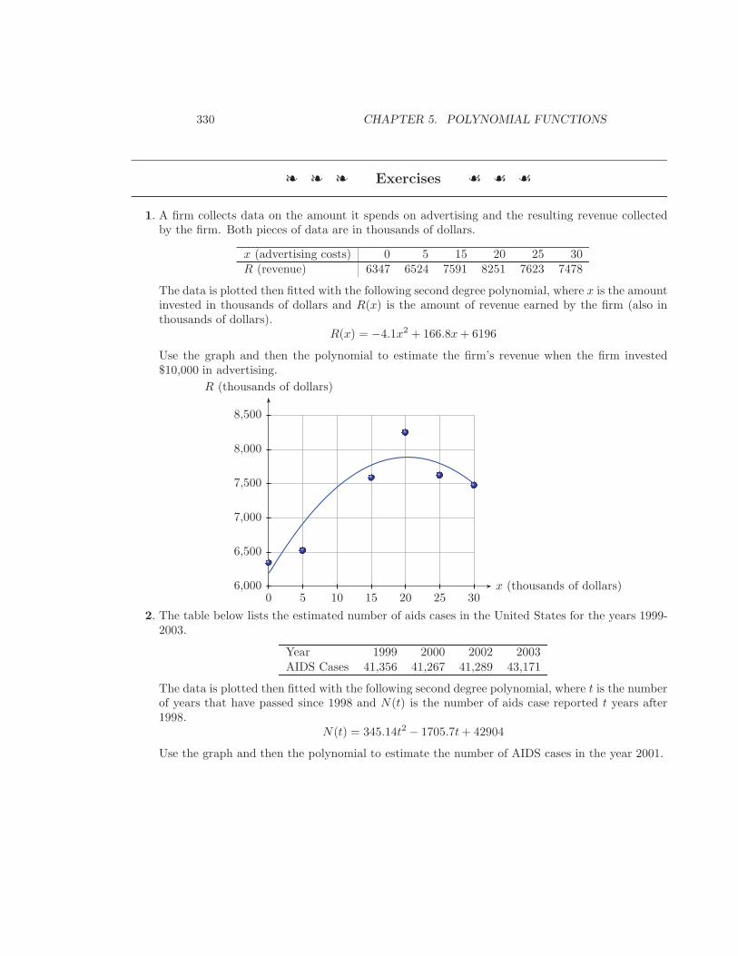
1. A firm collects data on the amount it spends on advertising and the resulting revenue collectedby the firm. Both pieces of data are in thousands of dollars.
x (advertising costs) 0 5 15 20 25 30R (revenue) 6347 6524 7591 8251 7623 7478
The data is plotted then fitted with the following second degree polynomial, where x is the amountinvested in thousands of dollars and R(x) is the amount of revenue earned by the firm (also inthousands of dollars).
R(x) = −4.1x2 + 166.8x+ 6196
Use the graph and then the polynomial to estimate the firm’s revenue when the firm invested$10,000 in advertising.
0 5 10 15 20 25 306,000
6,500
7,000
7,500
8,000
8,500
x (thousands of dollars)
R (thousands of dollars)
2. The table below lists the estimated number of aids cases in the United States for the years 1999-2003.
Year 1999 2000 2002 2003AIDS Cases 41,356 41,267 41,289 43,171
The data is plotted then fitted with the following second degree polynomial, where t is the numberof years that have passed since 1998 and N(t) is the number of aids case reported t years after1998.
N(t) = 345.14t2 − 1705.7t+ 42904
Use the graph and then the polynomial to estimate the number of AIDS cases in the year 2001.

5.3. APPLICATIONS OF POLYNOMIALS 331
0 1 2 3 4 5 640,000
41,000
42,000
43,000
44,000
45,000
t (Years since 1998)
N (Number of AID cases)
3. The following table records the concentration (in milligrams per liter) of medication in a patient’sblood after indicated times have passed.
Time (Hours) 0 0.5 1 1.5 2.5Concentration (mg/L) 0 78.1 99.8 84.4 15.6
The data is plotted then fitted with the following second degree polynomial, where t is the numberof hours that have passed since taking the medication and C(t) is the concentration (in milligramsper liter) of the medication in the patient’s blood after t hours have passed.
C(t) = −56.214t2 + 139.31t+ 9.35
Use the graph and then the polynomial to estimate the the concentration of medication in thepatient’s blood 2 hours after taking the medication.
0 1 2 30
20
40
60
80
100
t (Hours)
C (mg/L)

332 CHAPTER 5. POLYNOMIAL FUNCTIONS
4. The following table records the population (in millions of people) of the United States for thegiven year.
Year 1900 1920 1940 1960 1980 2000 2010Population (millions) 76.2 106.0 132.2 179.3 226.5 281.4 307.7
The data is plotted then fitted with the following second degree polynomial, where t is the numberof years that have passed since 1990 and P (t) is the population (in millions) t years after 1990.
P (t) = 0.008597t2 + 1, 1738t+ 76.41
Use the graph and then the polynomial to estimate the the population of the United States inthe year 1970.
0 20 40 60 80 100 12050
100
150
200
250
300
350
t (years since 1990)
P (millions of people)
5. If a projectile is launched with an ini-tial velocity of 457 meters per second(457m/s) from a rooftop 75 meters (75m)above ground level, at what time will theprojectile first reach a height of 6592 me-ters (6592m)? Round your answer tothe nearest second. Note: The accelera-tion due to gravity near the earth’s sur-face is 9.8 meters per second per second(9.8m/s2).
6. If a projectile is launched with an ini-tial velocity of 236 meters per second(236m/s) from a rooftop 15 meters (15m)
above ground level, at what time will theprojectile first reach a height of 1838 me-ters (1838m)? Round your answer tothe nearest second. Note: The accelera-tion due to gravity near the earth’s sur-face is 9.8 meters per second per second(9.8m/s2).
7. If a projectile is launched with an ini-tial velocity of 229 meters per second(229m/s) from a rooftop 58 meters (58m)above ground level, at what time will theprojectile first reach a height of 1374 me-ters (1374m)? Round your answer to

5.3. APPLICATIONS OF POLYNOMIALS 333
the nearest second. Note: The accelera-tion due to gravity near the earth’s sur-face is 9.8 meters per second per second(9.8m/s2).
8. If a projectile is launched with an ini-tial velocity of 234 meters per second(234m/s) from a rooftop 16 meters (16m)
above ground level, at what time will theprojectile first reach a height of 1882 me-ters (1882m)? Round your answer tothe nearest second. Note: The accelera-tion due to gravity near the earth’s sur-face is 9.8 meters per second per second(9.8m/s2).
In Exercises 9-12, first use an algebraic technique to find the zero of the given function, then usethe 2:zero utility on your graphing calculator to locate the zero of the function. Use the CalculatorSubmission Guidelines when reporting the zero found using your graphing calculator.
9. f(x) = 3.25x− 4.875
10. f(x) = 3.125− 2.5x
11. f(x) = 3.9− 1.5x
12. f(x) = 0.75x+ 2.4
13. If a projectile is launched with an ini-tial velocity of 203 meters per second(203m/s) from a rooftop 52 meters (52m)above ground level, at what time will theprojectile return to ground level? Roundyour answer to the nearest tenth of a sec-ond. Note: The acceleration due to grav-ity near the earth’s surface is 9.8 metersper second per second (9.8m/s2).
14. If a projectile is launched with an ini-tial velocity of 484 meters per second(484m/s) from a rooftop 17 meters (17m)above ground level, at what time will theprojectile return to ground level? Roundyour answer to the nearest tenth of a sec-ond. Note: The acceleration due to grav-ity near the earth’s surface is 9.8 metersper second per second (9.8m/s2).
15. If a projectile is launched with an ini-tial velocity of 276 meters per second(276m/s) from a rooftop 52 meters (52m)above ground level, at what time will theprojectile return to ground level? Roundyour answer to the nearest tenth of a sec-ond. Note: The acceleration due to grav-ity near the earth’s surface is 9.8 metersper second per second (9.8m/s2).
16. If a projectile is launched with an ini-tial velocity of 204 meters per second(204m/s) from a rooftop 92 meters (92m)above ground level, at what time will theprojectile return to ground level? Roundyour answer to the nearest tenth of a sec-ond. Note: The acceleration due to grav-ity near the earth’s surface is 9.8 metersper second per second (9.8m/s2).
§ § § Answers § § §
1. Approximately $7,454,000
3. Approximately 63 mg/L
5. 17.6 seconds
7. 6.7 seconds
9. Zero: 1.5
11. Zero: 2.6
13. 41.7 seconds
15. 56.5 seconds