5.2 Noncorrelated Subqueries - … · Web view05-10-2017 · FORD. As this query ... Whether you would actually want to use such a strategy in your code is up to you; ... 5.5 Subquery

5.1 What Is a Subquery?As we mentioned in Chapter 1, a subquery is a SELECT statement that is nested within another SQL statement. For the purpose of this discussion, we will call the SQL statement that contains a subquery the containing statement. Subqueries are executed prior to execution of their containing SQL statement (see Section 5.3 later in this chapter for the exception to this rule), and the result set generated by a subquery is discarded after its containing SQL statement has finished execution. Thus, a subquery can be thought of as a temporary table with statement scope.Syntactically, subqueries are enclosed within parentheses. For example, the following SELECT statement contains a simple subquery in its WHERE clause:SELECT * FROM customer

WHERE cust_nbr = (SELECT 123 FROM dual);

The subquery in this statement is absurdly simple, and completely unnecessary, but it does serve to illustrate a point. When this statement is executed, the subquery is evaluated first. The result of that subquery then becomes a value in the WHERE clause expression:SELECT * FROM customer

WHERE cust_nbr = 123;

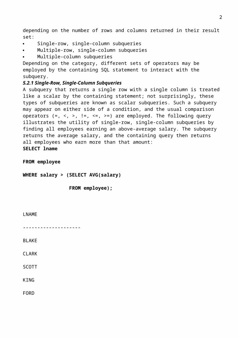
With the subquery out of the way, the containing query can now be evaluated. In this case, it would bring back information about customer number 123.Subqueries are most often found in the WHERE clause of a SELECT, UPDATE, or DELETE statement, as well as in the SET clause of an UPDATE statement. A subquery may either be correlated with its containing SQL statement, meaning that it references one or more columns from the containing statement, or it might reference nothing outside itself, in which case it is called a noncorrelated subquery. A less commonly used but powerful variety of subquery, called the inline view, occurs in the FROM clause of a SELECT statement. Inline views are always noncorrelated; they are evaluated first and behave like unindexed tables cached in memory for the remainder of the query.5.2 Noncorrelated SubqueriesNoncorrelated subqueries allow each row from the containing SQL statement to be compared to a set of values. You can divide noncorrelated subqueries into the following three categories, depending on the number of rows and columns returned in their result set: Single-row, single-column subqueries Multiple-row, single-column subqueries Multiple-column subqueriesDepending on the category, different sets of operators may be employed by the containing SQL statement to interact with the subquery.5.2.1 Single-Row, Single-Column SubqueriesA subquery that returns a single row with a single column is treated like a scalar by the containing statement; not surprisingly, these types of subqueries are known as scalar subqueries. Such a subquery may appear on either side of a condition, and the usual comparison operators (=, <, >, !=, <=, >=) are employed. The following query illustrates the utility of single-row, single-column subqueries by finding all employees earning an above-average salary. The subquery returns the average salary, and the containing query then returns all employees who earn more than that amount:SELECT lname

FROM employee

WHERE salary > (SELECT AVG(salary)

FROM employee);

2

LNAME

--------------------

BLAKE

CLARK

SCOTT

KING

FORD

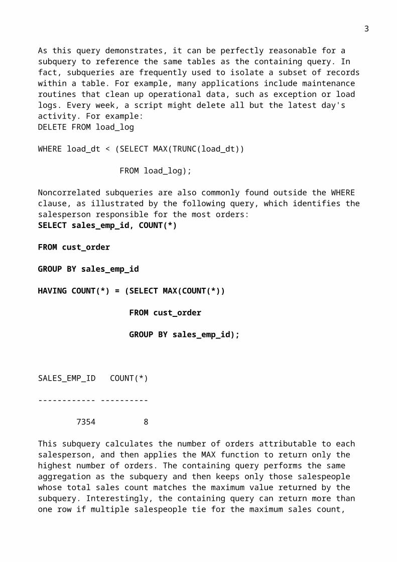
As this query demonstrates, it can be perfectly reasonable for a subquery to reference the same tables as the containing query. In fact, subqueries are frequently used to isolate a subset of records within a table. For example, many applications include maintenance routines that clean up operational data, such as exception or load logs. Every week, a script might delete all but the latest day's activity. For example:DELETE FROM load_log

WHERE load_dt < (SELECT MAX(TRUNC(load_dt))

FROM load_log);

Noncorrelated subqueries are also commonly found outside the WHERE clause, as illustrated by the following query, which identifies the salesperson responsible for the most orders:SELECT sales_emp_id, COUNT(*)

FROM cust_order

GROUP BY sales_emp_id

HAVING COUNT(*) = (SELECT MAX(COUNT(*))

FROM cust_order

GROUP BY sales_emp_id);

SALES_EMP_ID COUNT(*)

------------ ----------

7354 8

This subquery calculates the number of orders attributable to each salesperson, and then applies the MAX function to return only the highest number of orders. The containing query performs the same

3

aggregation as the subquery and then keeps only those salespeople whose total sales count matches the maximum value returned by the subquery. Interestingly, the containing query can return more than one row if multiple salespeople tie for the maximum sales count, while the subquery is guaranteed to return a single row and column. If it seems wasteful that the subquery and containing query both perform the same aggregation, it is; see Chapter 14 for more efficient ways to handle these types of queries.So far, you have seen scalar subqueries in the WHERE and HAVING clauses of SELECT statements, along with the WHERE clause of a DELETE statement. Before delving deeper into the different types of subqueries, let's explore where else subqueries can and can't be utilized in SQL statements: The FROM clause may contain any type of noncorrelated subquery. The SELECT and ORDER BY clauses may contain scalar subqueries. The GROUP BY clause may not contain subqueries. The START WITH and CONNECT BY clauses, used for querying hierarchical data, may contain subqueries and will be examined in detail in Chapter 8. The WITH clause contains a named noncorrelated subquery that can be referenced multiple times within the containing query but executes only once (see the examples later in this chapter). The USING clause of a MERGE statement may contain noncorrelated subqueries. The SET clause of UPDATE statements may contain scalar or single-row, multiple-column subqueries. INSERT statements may contain scalar subqueries in the VALUES clause.5.2.2 Multiple-Row, Single-Column SubqueriesNow that you know how to use single-row, single-column subqueries, let's explore how to use subqueries that return multiple rows. When a subquery returns more than one row, it is not possible to use only comparison operators, since a single value cannot be directly compared to a set of values. However, a single value can be compared to each value in a set. To accomplish this, the special keywords ANY and ALL are used with comparison operators to determine if a value is equal to (or less than, greater than, etc.) any member of the set or all members of the set. Consider the following query:SELECT fname, lname

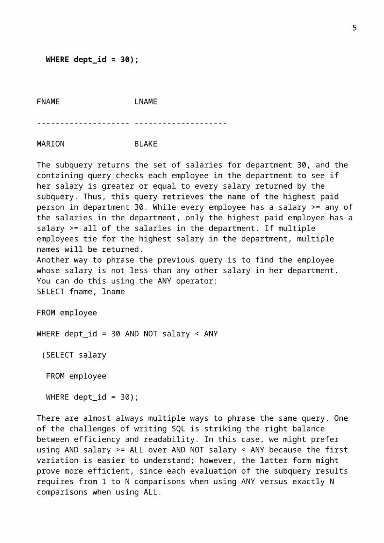
FROM employee

WHERE dept_id = 30 AND salary >= ALL

(SELECT salary

FROM employee

WHERE dept_id = 30);

FNAME LNAME

-------------------- --------------------

MARION BLAKE

The subquery returns the set of salaries for department 30, and the containing query checks each employee in the department to see if her salary is greater or equal to every salary returned by the subquery. Thus, this query retrieves the name of the highest paid person in department 30. While every employee has a salary >= any of the salaries in the department, only the highest paid employee has a

mk:@MSITStore:G:%5C_____Gramatas_un_pasutisana%5CSQL%5CPamati%5C_A_Beaulieu_Mastering_Oracle_SQL_2004.chm::/0596006322/mastorasql2-CHP-8.html#mastorasql2-CHP-8


4

salary >= all of the salaries in the department. If multiple employees tie for the highest salary in the department, multiple names will be returned.Another way to phrase the previous query is to find the employee whose salary is not less than any other salary in her department. You can do this using the ANY operator:SELECT fname, lname

FROM employee

WHERE dept_id = 30 AND NOT salary < ANY

(SELECT salary

FROM employee

WHERE dept_id = 30);

There are almost always multiple ways to phrase the same query. One of the challenges of writing SQL is striking the right balance between efficiency and readability. In this case, we might prefer using AND salary >= ALL over AND NOT salary < ANY because the first variation is easier to understand; however, the latter form might prove more efficient, since each evaluation of the subquery results requires from 1 to N comparisons when using ANY versus exactly N comparisons when using ALL.

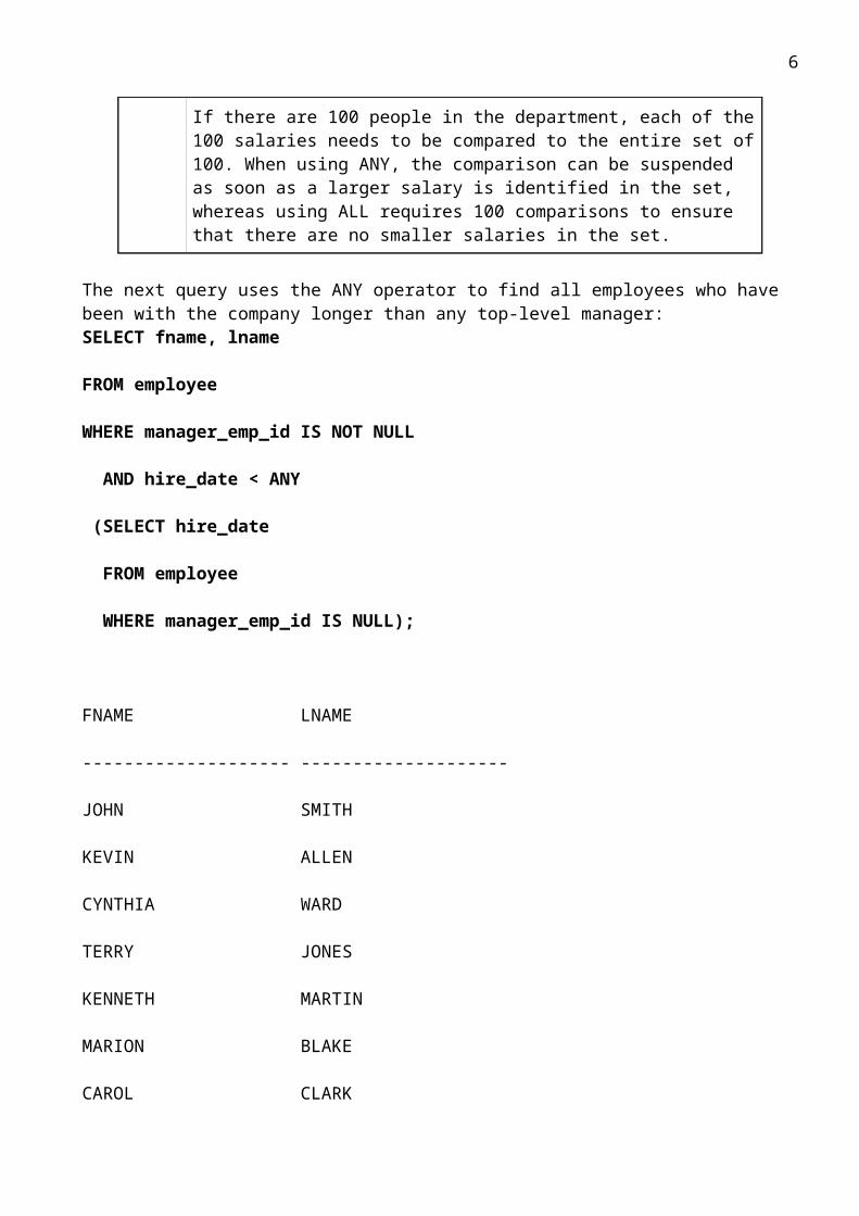
If there are 100 people in the department, each of the 100 salaries needs to be compared to the entire set of 100. When using ANY, the comparison can be suspended as soon as a larger salary is identified in the set, whereas using ALL requires 100 comparisons to ensure that there are no smaller salaries in the set.

The next query uses the ANY operator to find all employees who have been with the company longer than any top-level manager:SELECT fname, lname

FROM employee

WHERE manager_emp_id IS NOT NULL

AND hire_date < ANY

(SELECT hire_date

FROM employee

WHERE manager_emp_id IS NULL);

FNAME LNAME

-------------------- --------------------

JOHN SMITH

5

KEVIN ALLEN

CYNTHIA WARD

TERRY JONES

KENNETH MARTIN

MARION BLAKE

CAROL CLARK

MARY TURNER

The subquery returns the set of hire dates for all top-level managers, and the containing query returns the names of non-top-level managers whose hire date is previous to any returned by the subquery.For the previous three queries, failure to include either the ANY or ALL operators may result in the following error:ORA-01427: single-row subquery returns more than one row

The wording of this error message is a bit confusing. After all, how can a single-row subquery return multiple rows? What the error message is trying to convey is that a multiple-row subquery has been identified where only a single-row subquery is allowed. If you are not absolutely certain that your subquery will return exactly one row, you must include ANY or ALL to ensure your code doesn't fail in the future.Along with ANY and ALL, you may also use the IN operator for working with multi-row subqueries. Using IN with a subquery is functionally equivalent to using = ANY, and returns TRUE if a match is found in the set returned by the subquery. The following query uses IN to postpone shipment of all orders containing parts that are not currently in stock:UPDATE cust_order

SET expected_ship_dt = TRUNC(SYSDATE) + 1

WHERE ship_dt IS NULL

AND order_nbr IN

(SELECT l.order_nbr

FROM line_item l INNER JOIN part p

ON l.part_nbr = p.part_nbr

WHERE p.inventory_qty = 0);

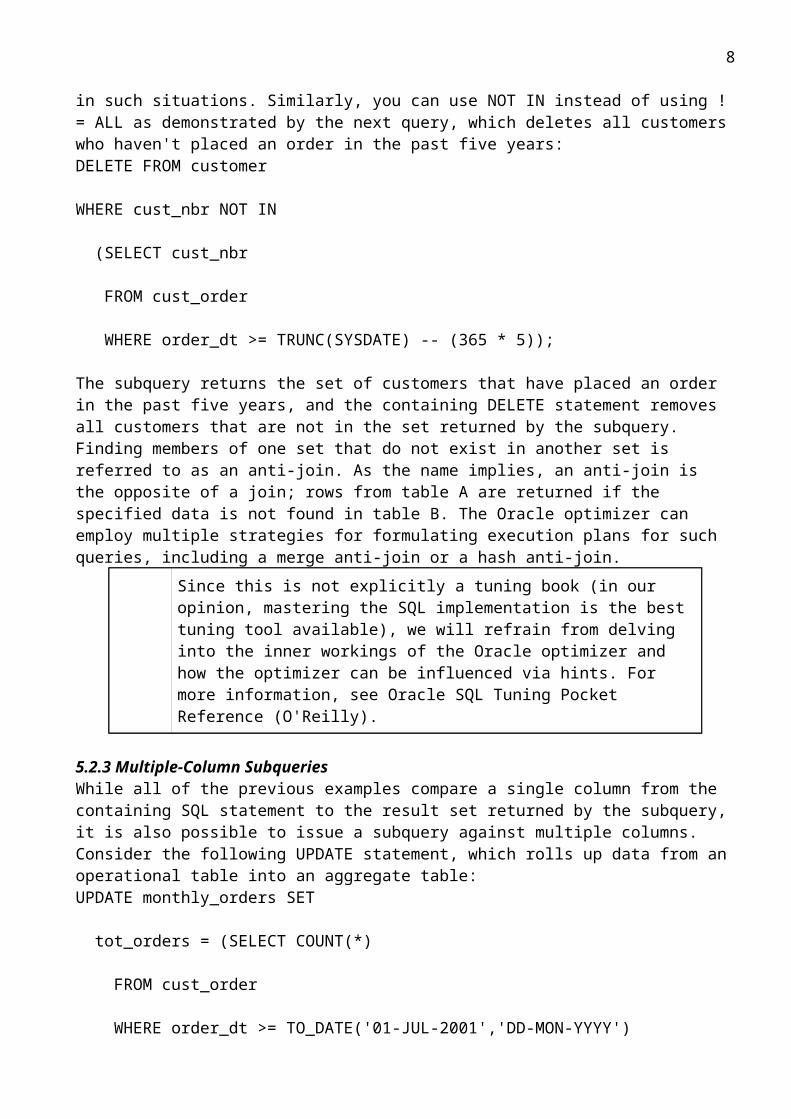
The subquery returns the set of orders requesting out-of-stock parts, and the containing UPDATE statement modifies the expected ship date of all orders in the set. We think you will agree that IN is more intuitive than = ANY, which is why IN is almost always used in such situations. Similarly, you can use NOT IN instead of using != ALL as demonstrated by the next query, which deletes all customers who haven't placed an order in the past five years:DELETE FROM customer

6

WHERE cust_nbr NOT IN

(SELECT cust_nbr

FROM cust_order

WHERE order_dt >= TRUNC(SYSDATE) -- (365 * 5));

The subquery returns the set of customers that have placed an order in the past five years, and the containing DELETE statement removes all customers that are not in the set returned by the subquery.Finding members of one set that do not exist in another set is referred to as an anti-join. As the name implies, an anti-join is the opposite of a join; rows from table A are returned if the specified data is not found in table B. The Oracle optimizer can employ multiple strategies for formulating execution plans for such queries, including a merge anti-join or a hash anti-join.

Since this is not explicitly a tuning book (in our opinion, mastering the SQL implementation is the best tuning tool available), we will refrain from delving into the inner workings of the Oracle optimizer and how the optimizer can be influenced via hints. For more information, see Oracle SQL Tuning Pocket Reference (O'Reilly).

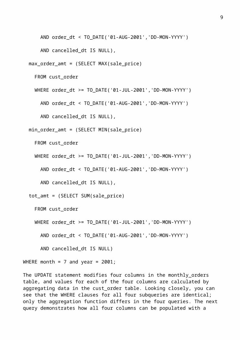
5.2.3 Multiple-Column SubqueriesWhile all of the previous examples compare a single column from the containing SQL statement to the result set returned by the subquery, it is also possible to issue a subquery against multiple columns. Consider the following UPDATE statement, which rolls up data from an operational table into an aggregate table:UPDATE monthly_orders SET

tot_orders = (SELECT COUNT(*)

FROM cust_order

WHERE order_dt >= TO_DATE('01-JUL-2001','DD-MON-YYYY')

AND order_dt < TO_DATE('01-AUG-2001','DD-MON-YYYY')

AND cancelled_dt IS NULL),

max_order_amt = (SELECT MAX(sale_price)

FROM cust_order




min_order_amt = (SELECT MIN(sale_price)

FROM cust_order

7




tot_amt = (SELECT SUM(sale_price)

FROM cust_order



AND cancelled_dt IS NULL)

WHERE month = 7 and year = 2001;

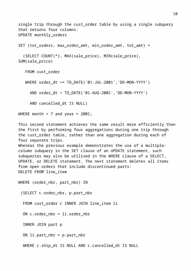
The UPDATE statement modifies four columns in the monthly_orders table, and values for each of the four columns are calculated by aggregating data in the cust_order table. Looking closely, you can see that the WHERE clauses for all four subqueries are identical; only the aggregation function differs in the four queries. The next query demonstrates how all four columns can be populated with a single trip through the cust_order table by using a single subquery that returns four columns:UPDATE monthly_orders

SET (tot_orders, max_order_amt, min_order_amt, tot_amt) =

(SELECT COUNT(*), MAX(sale_price), MIN(sale_price), SUM(sale_price)

FROM cust_order



AND cancelled_dt IS NULL)

WHERE month = 7 and year = 2001;

This second statement achieves the same result more efficiently than the first by performing four aggregations during one trip through the cust_order table, rather than one aggregation during each of four separate trips.Whereas the previous example demonstrates the use of a multiple-column subquery in the SET clause of an UPDATE statement, such subqueries may also be utilized in the WHERE clause of a SELECT, UPDATE, or DELETE statement. The next statement deletes all items from open orders that include discontinued parts:DELETE FROM line_item

WHERE (order_nbr, part_nbr) IN

(SELECT c.order_nbr, p.part_nbr

8

FROM cust_order c INNER JOIN line_item li

ON c.order_nbr = li.order_nbr

INNER JOIN part p

ON li.part_nbr = p.part_nbr

WHERE c.ship_dt IS NULL AND c.cancelled_dt IS NULL

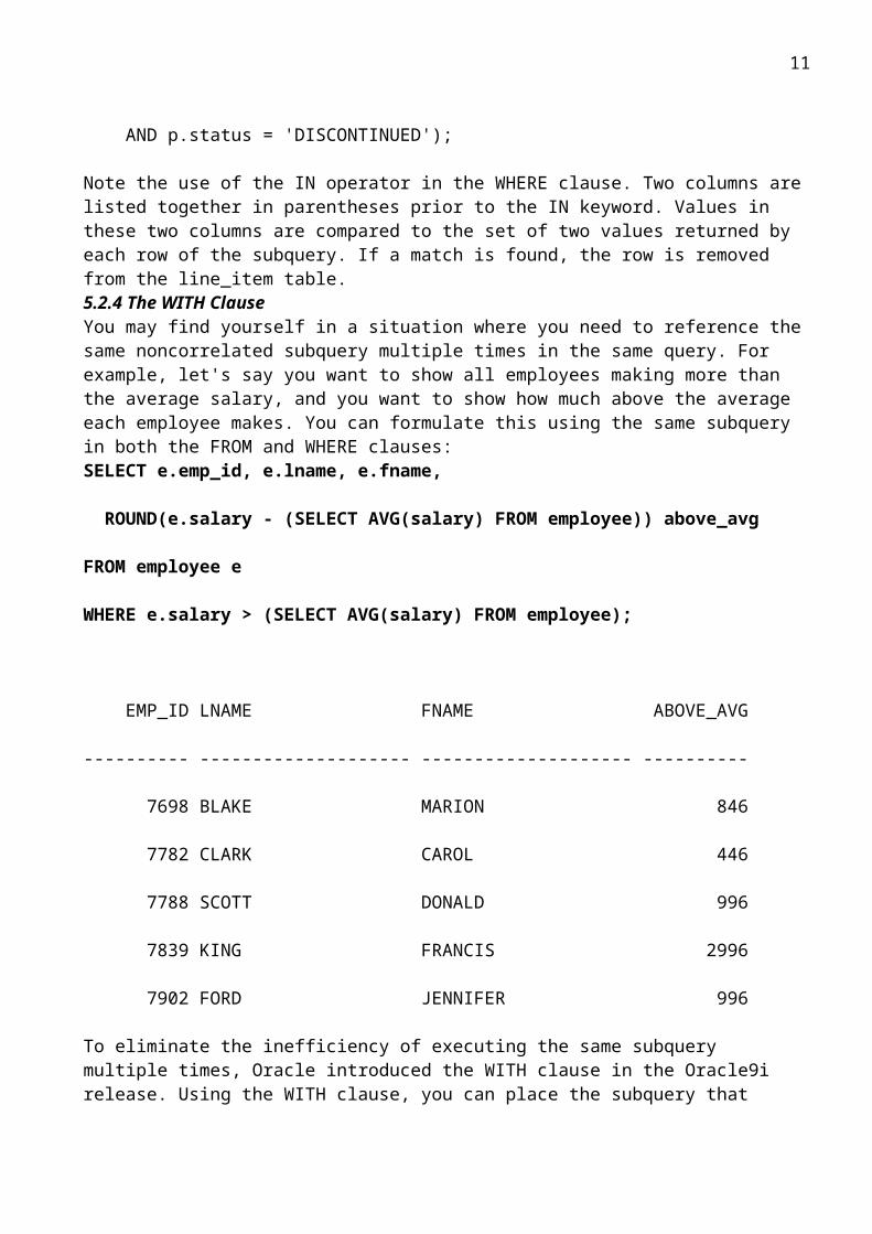
AND p.status = 'DISCONTINUED');

Note the use of the IN operator in the WHERE clause. Two columns are listed together in parentheses prior to the IN keyword. Values in these two columns are compared to the set of two values returned by each row of the subquery. If a match is found, the row is removed from the line_item table.5.2.4 The WITH ClauseYou may find yourself in a situation where you need to reference the same noncorrelated subquery multiple times in the same query. For example, let's say you want to show all employees making more than the average salary, and you want to show how much above the average each employee makes. You can formulate this using the same subquery in both the FROM and WHERE clauses:SELECT e.emp_id, e.lname, e.fname,

ROUND(e.salary - (SELECT AVG(salary) FROM employee)) above_avg

FROM employee e

WHERE e.salary > (SELECT AVG(salary) FROM employee);

EMP_ID LNAME FNAME ABOVE_AVG

---------- -------------------- -------------------- ----------

7698 BLAKE MARION 846

7782 CLARK CAROL 446

7788 SCOTT DONALD 996

7839 KING FRANCIS 2996

7902 FORD JENNIFER 996

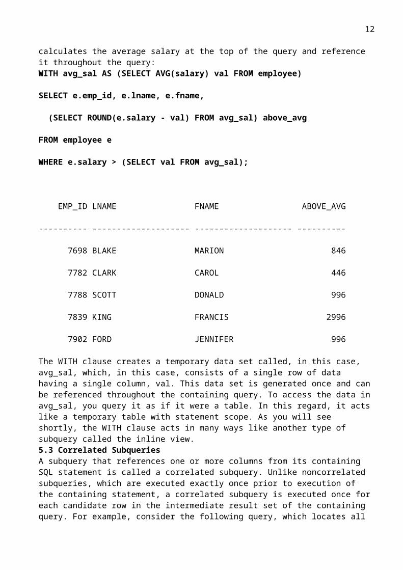
To eliminate the inefficiency of executing the same subquery multiple times, Oracle introduced the WITH clause in the Oracle9i release. Using the WITH clause, you can place the subquery that calculates the average salary at the top of the query and reference it throughout the query:WITH avg_sal AS (SELECT AVG(salary) val FROM employee)

SELECT e.emp_id, e.lname, e.fname,

(SELECT ROUND(e.salary - val) FROM avg_sal) above_avg

9

FROM employee e

WHERE e.salary > (SELECT val FROM avg_sal);

EMP_ID LNAME FNAME ABOVE_AVG

---------- -------------------- -------------------- ----------

7698 BLAKE MARION 846

7782 CLARK CAROL 446

7788 SCOTT DONALD 996

7839 KING FRANCIS 2996

7902 FORD JENNIFER 996

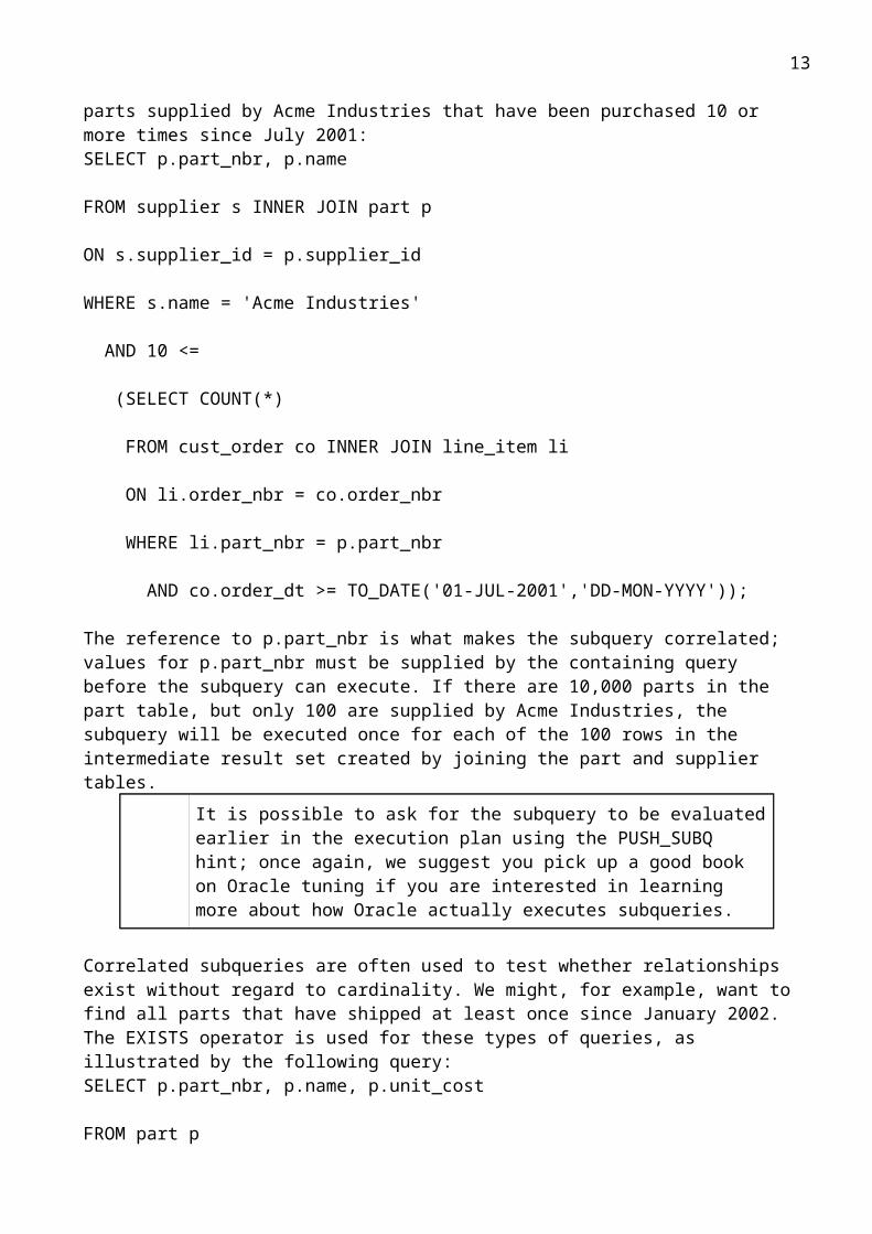
The WITH clause creates a temporary data set called, in this case, avg_sal, which, in this case, consists of a single row of data having a single column, val. This data set is generated once and can be referenced throughout the containing query. To access the data in avg_sal, you query it as if it were a table. In this regard, it acts like a temporary table with statement scope. As you will see shortly, the WITH clause acts in many ways like another type of subquery called the inline view.5.3 Correlated SubqueriesA subquery that references one or more columns from its containing SQL statement is called a correlated subquery. Unlike noncorrelated subqueries, which are executed exactly once prior to execution of the containing statement, a correlated subquery is executed once for each candidate row in the intermediate result set of the containing query. For example, consider the following query, which locates all parts supplied by Acme Industries that have been purchased 10 or more times since July 2001:SELECT p.part_nbr, p.name

FROM supplier s INNER JOIN part p

ON s.supplier_id = p.supplier_id

WHERE s.name = 'Acme Industries'

AND 10 <=

(SELECT COUNT(*)

FROM cust_order co INNER JOIN line_item li

ON li.order_nbr = co.order_nbr

WHERE li.part_nbr = p.part_nbr

AND co.order_dt >= TO_DATE('01-JUL-2001','DD-MON-YYYY'));

10

The reference to p.part_nbr is what makes the subquery correlated; values for p.part_nbr must be supplied by the containing query before the subquery can execute. If there are 10,000 parts in the part table, but only 100 are supplied by Acme Industries, the subquery will be executed once for each of the 100 rows in the intermediate result set created by joining the part and supplier tables.

It is possible to ask for the subquery to be evaluated earlier in the execution plan using the PUSH_SUBQ hint; once again, we suggest you pick up a good book on Oracle tuning if you are interested in learning more about how Oracle actually executes subqueries.

Correlated subqueries are often used to test whether relationships exist without regard to cardinality. We might, for example, want to find all parts that have shipped at least once since January 2002. The EXISTS operator is used for these types of queries, as illustrated by the following query:SELECT p.part_nbr, p.name, p.unit_cost

FROM part p

WHERE EXISTS

(SELECT 1

FROM line_item li INNER JOIN cust_order co

ON li.order_nbr = co.order_nbr

WHERE li.part_nbr = p.part_nbr

AND co.ship_dt >= TO_DATE('01-JAN-2002','DD-MON-YYYY'));

As long as the subquery returns one or more rows, the EXISTS condition is satisfied without regard for how many rows were actually returned by the subquery. Since the EXISTS operator returns TRUE or FALSE depending on the number of rows returned by the subquery, the actual columns returned by the subquery are irrelevant. The SELECT clause requires at least one column, however, so it is common practice to use either the literal "1" or the wildcard "*".Conversely, you can test whether a relationship does not exist:UPDATE customer c

SET c.inactive_ind = 'Y', c.inactive_dt = TRUNC(SYSDATE)

WHERE c.inactive_dt IS NULL

AND NOT EXISTS (SELECT 1 FROM cust_order co

WHERE co.cust_nbr = c.cust_nbr

AND co.order_dt > TRUNC(SYSDATE) -- 365);

This statement makes all customer records inactive for those customers who haven't placed an order in the past year. Such queries are commonly found in maintenance routines. For example, foreign key constraints might prevent child records from referring to a nonexistent parent, but it is possible to have

11

parent records without children. If business rules prohibit this situation, you might run a utility each week that removes these records, as in:DELETE FROM cust_order co

WHERE co.order_dt > TRUNC(SYSDATE) -- 7

AND co.cancelled_dt IS NULL

AND NOT EXISTS

(SELECT 1 FROM line_item li

WHERE li.order_nbr = co.order_nbr);

A query that includes a correlated subquery using the EXISTS operator is referred to as a semi-join. A semi-join includes rows in table A for which corresponding data is found one or more times in table B. Thus, the size of the final result set is unaffected by the number of matches found in table B. Similar to the anti-join discussed earlier, the Oracle optimizer can employ multiple strategies for formulating execution plans for such queries, including a merge semi-join or a hash semi-join.Although they are very often used together, the use of correlated subqueries does not require the EXISTS operator. If your database design includes denormalized columns, for example, you might run nightly routines to recalculate the denormalized data, as in:UPDATE customer c

SET (c.tot_orders, c.last_order_dt) =

(SELECT COUNT(*), MAX(co.order_dt)

FROM cust_order co


AND co.cancelled_dt IS NULL);

Because a SET clause assigns values to columns in the table, the only operator allowed is =. The subquery returns exactly one row (thanks to the aggregation functions), so the results may be safely assigned to the target columns. Rather than recalculating the entire sum each day, a more efficient method might be to update only those customers who placed orders today:UPDATE customer c SET (c.tot_orders, c.last_order_dt) =

(SELECT c.tot_orders + COUNT(*), MAX(co.order_dt)

FROM cust_order co


AND co.cancelled_dt IS NULL

AND co.order_dt >= TRUNC(SYSDATE))

WHERE c.cust_nbr IN

12

(SELECT co.cust_nbr

FROM cust_order co

WHERE co.order_dt >= TRUNC(SYSDATE)

AND co.cancelled_dt IS NULL);

As the previous statement shows, data from the containing query can be used for other purposes in the correlated subquery than just join conditions in the WHERE clause. In this example, the SELECT clause of the correlated subquery adds today's sales totals to the previous value of tot_orders in the customer table to arrive at the new value.Along with the WHERE clause of SELECT, UPDATE, and DELETE statements, and the SET clause of UPDATE statements, another potent use of correlated subqueries is in the SELECT clause, as illustrated by the following:SELECT d.dept_id, d.name,

(SELECT COUNT(*) FROM employee e

WHERE e.dept_id = d.dept_id) empl_cnt

FROM department d;

DEPT_ID NAME EMPL_CNT

---------- -------------------- ----------

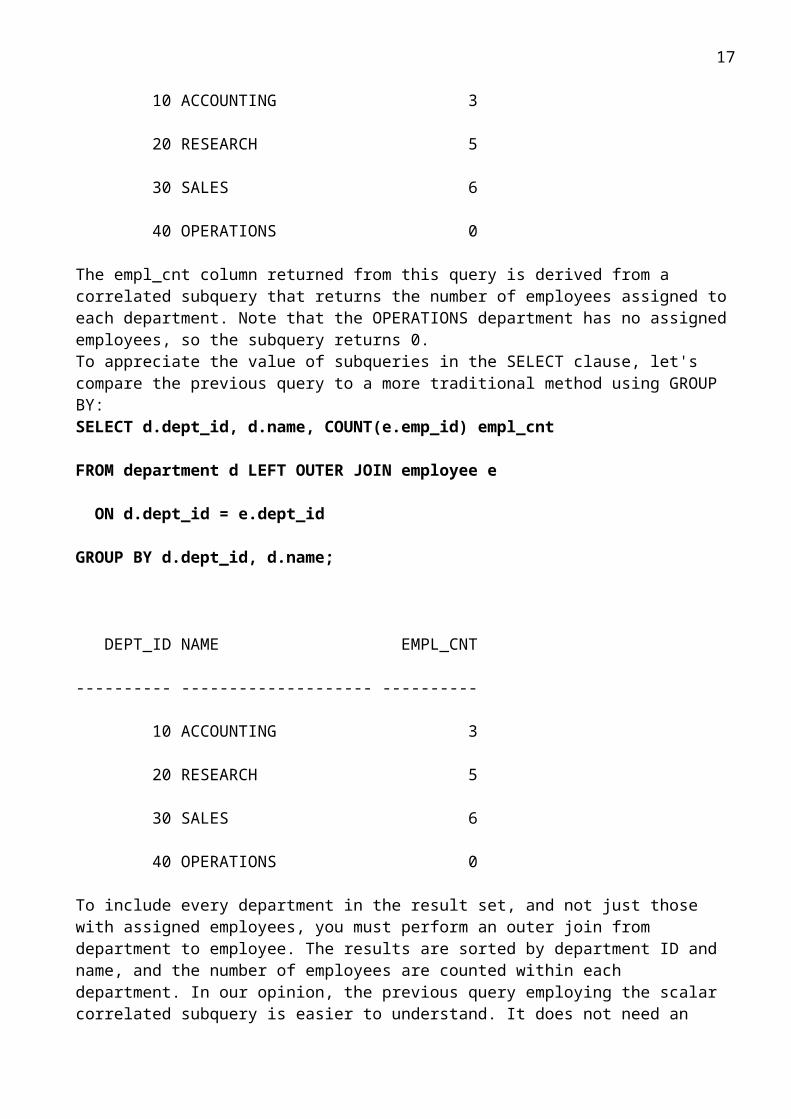
10 ACCOUNTING 3

20 RESEARCH 5

30 SALES 6

40 OPERATIONS 0

The empl_cnt column returned from this query is derived from a correlated subquery that returns the number of employees assigned to each department. Note that the OPERATIONS department has no assigned employees, so the subquery returns 0.To appreciate the value of subqueries in the SELECT clause, let's compare the previous query to a more traditional method using GROUP BY:SELECT d.dept_id, d.name, COUNT(e.emp_id) empl_cnt

FROM department d LEFT OUTER JOIN employee e

ON d.dept_id = e.dept_id

GROUP BY d.dept_id, d.name;

13

DEPT_ID NAME EMPL_CNT

---------- -------------------- ----------

10 ACCOUNTING 3

20 RESEARCH 5

30 SALES 6

40 OPERATIONS 0

To include every department in the result set, and not just those with assigned employees, you must perform an outer join from department to employee. The results are sorted by department ID and name, and the number of employees are counted within each department. In our opinion, the previous query employing the scalar correlated subquery is easier to understand. It does not need an outer join (or any join at all), and does not necessitate a sort operation, making it an attractive alternative to the GROUP BY version.5.4 Inline ViewsMost texts covering SQL define the FROM clause of a SELECT statement as containing a list of tables and/or views. Please abandon this definition and replace it with the following:The FROM clause contains a list of data sets.In this light, it is easy to see how the FROM clause can contain tables (permanent data sets), views (virtual data sets), and SELECT statements (temporary data sets). SELECT statements, or inline views as mentioned earlier, are one of the most powerful, yet underutilized features of Oracle SQL.

In our opinion, the name "inline view" is confusing and tends to intimidate people. Since it is a subquery that executes prior to the containing query, a more palatable name might have been "pre-query."

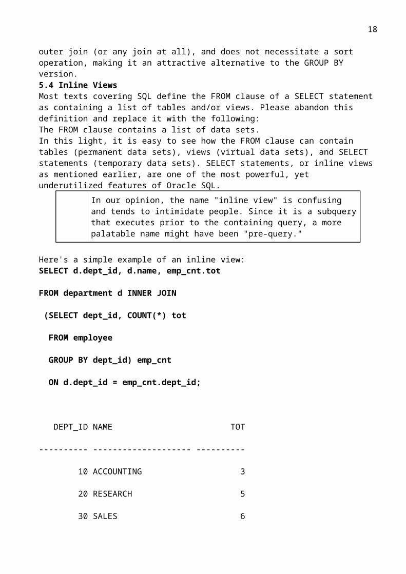
Here's a simple example of an inline view:SELECT d.dept_id, d.name, emp_cnt.tot

FROM department d INNER JOIN

(SELECT dept_id, COUNT(*) tot

FROM employee

GROUP BY dept_id) emp_cnt

ON d.dept_id = emp_cnt.dept_id;

DEPT_ID NAME TOT

---------- -------------------- ----------

10 ACCOUNTING 3

20 RESEARCH 5

14

30 SALES 6

In this example, the FROM clause references the department table and an inline view called emp_cnt, which calculates the number of employees in each department. The two sets are joined using dept_id and the ID, name, and employee count are returned for each department. While this example is fairly simple, inline views allow you to do things in a single query that might otherwise require multiple select statements or a procedural language to accomplish.5.4.1 Inline View BasicsBecause the result set from an inline view is referenced by other elements of the containing query, you must give your inline view a name and provide aliases for all ambiguous columns. In the previous example, the inline view was given the name "emp_cnt", and the alias "tot" was assigned to the COUNT(*) column. Similar to other types of subqueries, inline views may join multiple tables, call built-in and user-defined functions, specify optimizer hints, and include GROUP BY, HAVING, and CONNECT BY clauses. Unlike other types of subqueries, an inline view may also contain an ORDER BY clause, which opens several interesting possibilities (see Section 5.5 later in the chapter for an example using ORDER BY in a subquery).Inline views are particularly useful when you need to combine data at different levels of aggregation. In the previous example, we needed to retrieve all rows from the department table and include aggregated data from the employee table, so we chose to do the aggregation within an inline view and join the results to the department table. Anyone involved in report generation or data warehouse extraction, transformation, and load (ETL) applications has doubtless encountered situations where data from various levels of aggregation needs to be combined; with inline views, you should be able to produce the desired results in a single SQL statement rather than having to break the logic into multiple pieces or write code in a procedural language.When considering using an inline view, ask yourself the following questions: What value does the inline view add to the readability and, more importantly, the performance of the containing query? How large will the result set generated by the inline view be? How often, if ever, will I have need of this particular data set?Generally, using an inline view should enhance the readability and performance of the query, and it should generate a manageable data set that is of no value to other statements or sessions; otherwise, you may want to consider building a permanent or temporary table so that you can share the data between sessions and build additional indexes as needed.5.4.2 Query ExecutionInline views are always executed prior to the containing query and, thus, may not reference columns from other tables or inline views from the same query. After execution, the containing query interacts with an inline view as if it were an unindexed, in-memory table. If inline views are nested, the innermost inline view is executed first, followed by the next-innermost inline view, and so on. Consider the following query:SELECT d.dept_id dept_id, d.name dept_name,

dept_orders.tot_orders tot_orders

FROM department d INNER JOIN

(SELECT e.dept_id dept_id, SUM(emp_orders.tot_orders) tot_orders

FROM employee e INNER JOIN

(SELECT sales_emp_id, COUNT(*) tot_orders

mk:@MSITStore:G:%5C_____Gramatas_un_pasutisana%5CSQL%5CPamati%5C_A_Beaulieu_Mastering_Oracle_SQL_2004.chm::/0596006322/mastorasql2-CHP-5-SECT-5.html#mastorasql2-CHP-5-SECT-5

15

FROM cust_order

WHERE order_dt >= TO_DATE('01-JAN-2001','DD-MON-YYYY')

AND cancelled_dt IS NULL


) emp_orders

ON e.emp_id = emp_orders.sales_emp_id

GROUP BY e.dept_id

) dept_orders

ON d.dept_id = dept_orders.dept_id;

DEPT_ID DEPT_NAME TOT_ORDERS

---------- -------------------- ----------

30 SALES 6

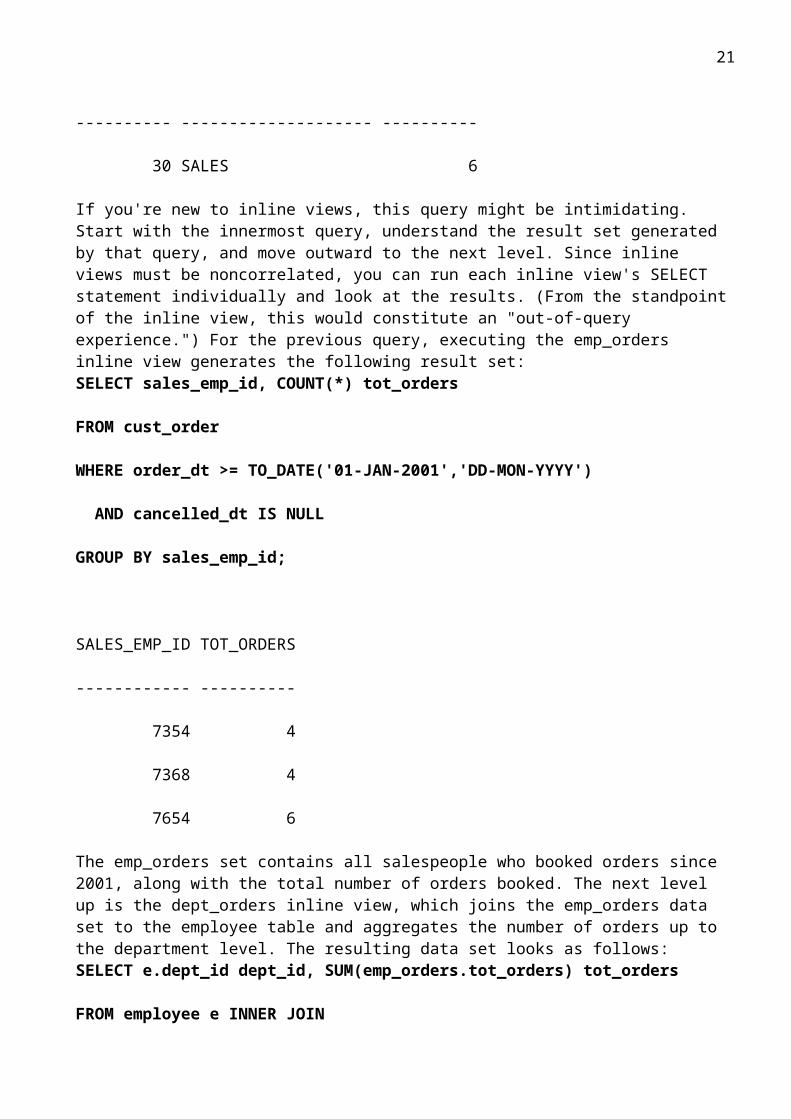
If you're new to inline views, this query might be intimidating. Start with the innermost query, understand the result set generated by that query, and move outward to the next level. Since inline views must be noncorrelated, you can run each inline view's SELECT statement individually and look at the results. (From the standpoint of the inline view, this would constitute an "out-of-query experience.") For the previous query, executing the emp_orders inline view generates the following result set:SELECT sales_emp_id, COUNT(*) tot_orders

FROM cust_order



GROUP BY sales_emp_id;

SALES_EMP_ID TOT_ORDERS

------------ ----------

7354 4

7368 4

16

7654 6

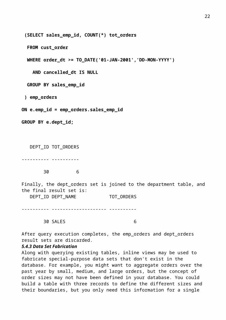
The emp_orders set contains all salespeople who booked orders since 2001, along with the total number of orders booked. The next level up is the dept_orders inline view, which joins the emp_orders data set to the employee table and aggregates the number of orders up to the department level. The resulting data set looks as follows:SELECT e.dept_id dept_id, SUM(emp_orders.tot_orders) tot_orders

FROM employee e INNER JOIN

(SELECT sales_emp_id, COUNT(*) tot_orders

FROM cust_order




) emp_orders

ON e.emp_id = emp_orders.sales_emp_id

GROUP BY e.dept_id;

DEPT_ID TOT_ORDERS

---------- ----------

30 6

Finally, the dept_orders set is joined to the department table, and the final result set is: DEPT_ID DEPT_NAME TOT_ORDERS

---------- -------------------- ----------

30 SALES 6

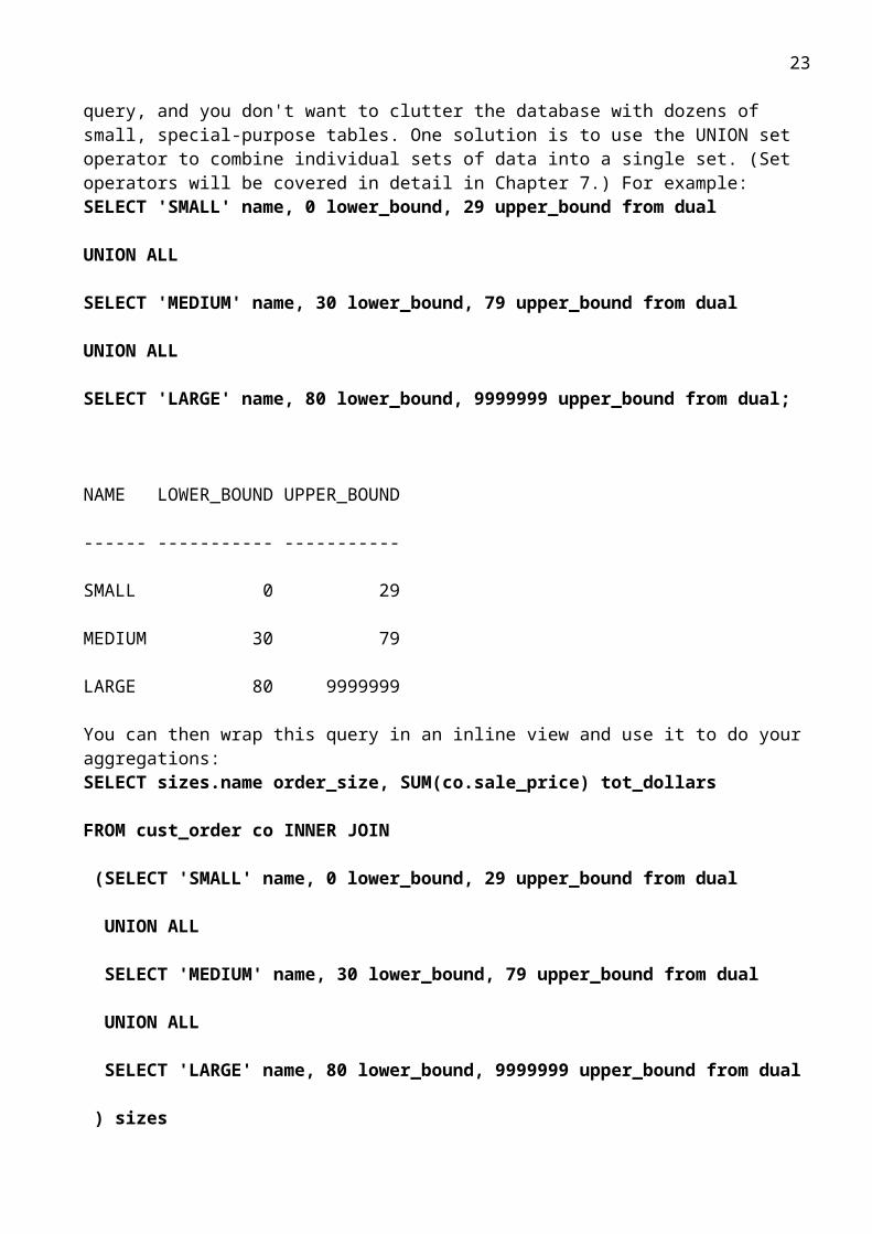
After query execution completes, the emp_orders and dept_orders result sets are discarded.5.4.3 Data Set FabricationAlong with querying existing tables, inline views may be used to fabricate special-purpose data sets that don't exist in the database. For example, you might want to aggregate orders over the past year by small, medium, and large orders, but the concept of order sizes may not have been defined in your database. You could build a table with three records to define the different sizes and their boundaries, but you only need this information for a single query, and you don't want to clutter the database with dozens of small, special-purpose tables. One solution is to use the UNION set operator to combine individual sets of data into a single set. (Set operators will be covered in detail in Chapter 7.) For example:SELECT 'SMALL' name, 0 lower_bound, 29 upper_bound from dual


17

UNION ALL

SELECT 'MEDIUM' name, 30 lower_bound, 79 upper_bound from dual

UNION ALL

SELECT 'LARGE' name, 80 lower_bound, 9999999 upper_bound from dual;

NAME LOWER_BOUND UPPER_BOUND

------ ----------- -----------

SMALL 0 29

MEDIUM 30 79

LARGE 80 9999999

You can then wrap this query in an inline view and use it to do your aggregations:SELECT sizes.name order_size, SUM(co.sale_price) tot_dollars

FROM cust_order co INNER JOIN

(SELECT 'SMALL' name, 0 lower_bound, 29 upper_bound from dual

UNION ALL


UNION ALL

SELECT 'LARGE' name, 80 lower_bound, 9999999 upper_bound from dual

) sizes

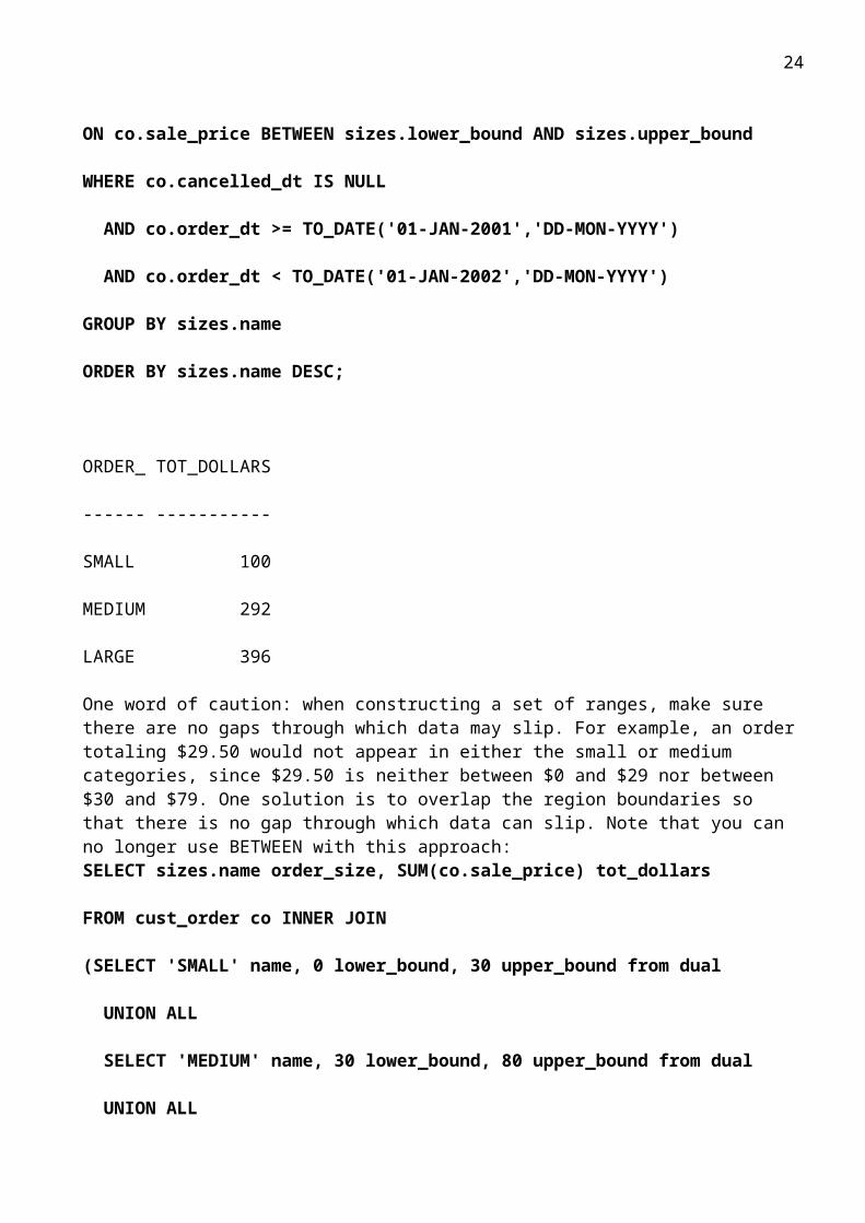
ON co.sale_price BETWEEN sizes.lower_bound AND sizes.upper_bound

WHERE co.cancelled_dt IS NULL

AND co.order_dt >= TO_DATE('01-JAN-2001','DD-MON-YYYY')

AND co.order_dt < TO_DATE('01-JAN-2002','DD-MON-YYYY')

GROUP BY sizes.name

ORDER BY sizes.name DESC;

18

ORDER_ TOT_DOLLARS

------ -----------

SMALL 100

MEDIUM 292

LARGE 396

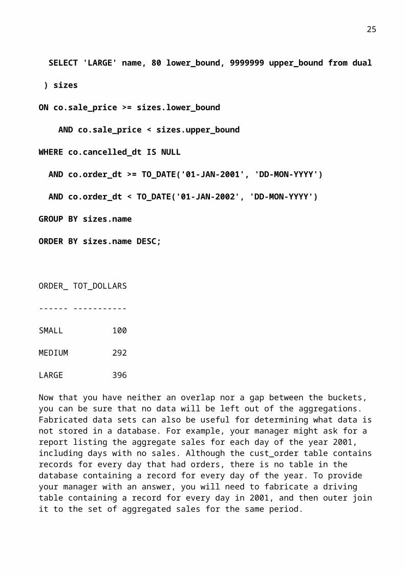
One word of caution: when constructing a set of ranges, make sure there are no gaps through which data may slip. For example, an order totaling $29.50 would not appear in either the small or medium categories, since $29.50 is neither between $0 and $29 nor between $30 and $79. One solution is to overlap the region boundaries so that there is no gap through which data can slip. Note that you can no longer use BETWEEN with this approach:SELECT sizes.name order_size, SUM(co.sale_price) tot_dollars


(SELECT 'SMALL' name, 0 lower_bound, 30 upper_bound from dual

UNION ALL


UNION ALL

SELECT 'LARGE' name, 80 lower_bound, 9999999 upper_bound from dual

) sizes

ON co.sale_price >= sizes.lower_bound

AND co.sale_price < sizes.upper_bound


AND co.order_dt >= TO_DATE('01-JAN-2001', 'DD-MON-YYYY')

AND co.order_dt < TO_DATE('01-JAN-2002', 'DD-MON-YYYY')

GROUP BY sizes.name

ORDER BY sizes.name DESC;

ORDER_ TOT_DOLLARS

------ -----------

SMALL 100

19

MEDIUM 292

LARGE 396

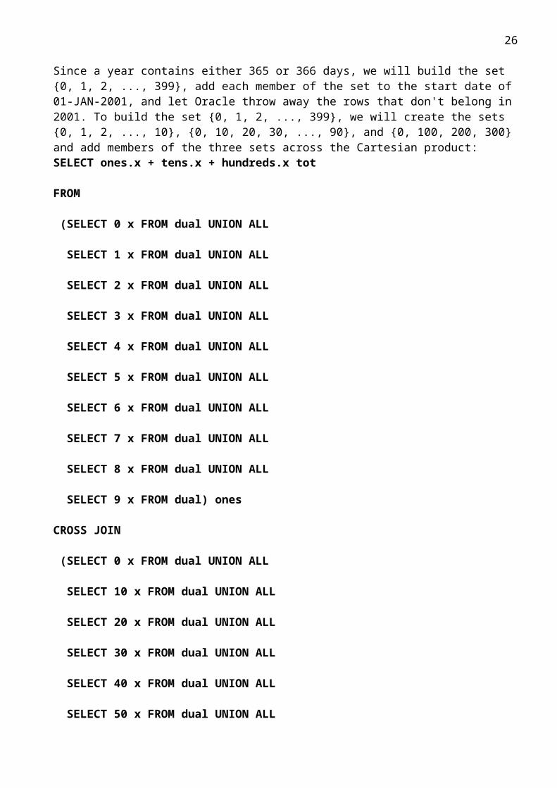
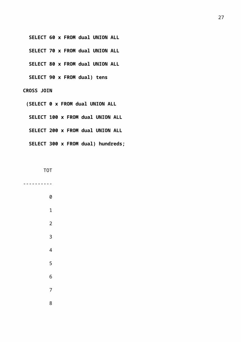
Now that you have neither an overlap nor a gap between the buckets, you can be sure that no data will be left out of the aggregations.Fabricated data sets can also be useful for determining what data is not stored in a database. For example, your manager might ask for a report listing the aggregate sales for each day of the year 2001, including days with no sales. Although the cust_order table contains records for every day that had orders, there is no table in the database containing a record for every day of the year. To provide your manager with an answer, you will need to fabricate a driving table containing a record for every day in 2001, and then outer join it to the set of aggregated sales for the same period.Since a year contains either 365 or 366 days, we will build the set {0, 1, 2, ..., 399}, add each member of the set to the start date of 01-JAN-2001, and let Oracle throw away the rows that don't belong in 2001. To build the set {0, 1, 2, ..., 399}, we will create the sets {0, 1, 2, ..., 10}, {0, 10, 20, 30, ..., 90}, and {0, 100, 200, 300} and add members of the three sets across the Cartesian product:SELECT ones.x + tens.x + hundreds.x tot

FROM

(SELECT 0 x FROM dual UNION ALL

SELECT 1 x FROM dual UNION ALL








SELECT 9 x FROM dual) ones

CROSS JOIN






20





SELECT 90 x FROM dual) tens

CROSS JOIN




SELECT 300 x FROM dual) hundreds;

TOT

----------

0

1

2

3

4

5

6

7

8

9

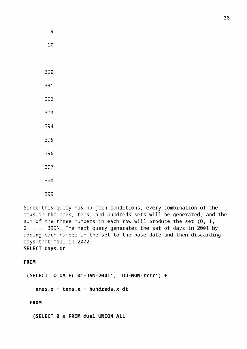
10

. . .

390

21

391

392

393

394

395

396

397

398

399

Since this query has no join conditions, every combination of the rows in the ones, tens, and hundreds sets will be generated, and the sum of the three numbers in each row will produce the set {0, 1, 2, ..., 399}. The next query generates the set of days in 2001 by adding each number in the set to the base date and then discarding days that fall in 2002:SELECT days.dt

FROM

(SELECT TO_DATE('01-JAN-2001', 'DD-MON-YYYY') +

ones.x + tens.x + hundreds.x dt

FROM










SELECT 9 x FROM dual) ones

22

CROSS JOIN










SELECT 90 x FROM dual) tens

CROSS JOIN




SELECT 300 x FROM dual) hundreds) days

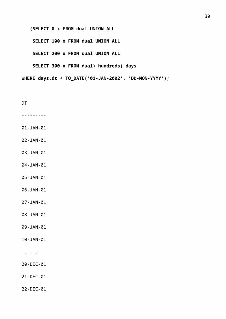
WHERE days.dt < TO_DATE('01-JAN-2002', 'DD-MON-YYYY');

DT

---------

01-JAN-01

02-JAN-01

03-JAN-01

04-JAN-01

05-JAN-01

06-JAN-01

23

07-JAN-01

08-JAN-01

09-JAN-01

10-JAN-01

. . .

20-DEC-01

21-DEC-01

22-DEC-01

23-DEC-01

24-DEC-01

25-DEC-01

26-DEC-01

27-DEC-01

28-DEC-01

29-DEC-01

30-DEC-01

31-DEC-01

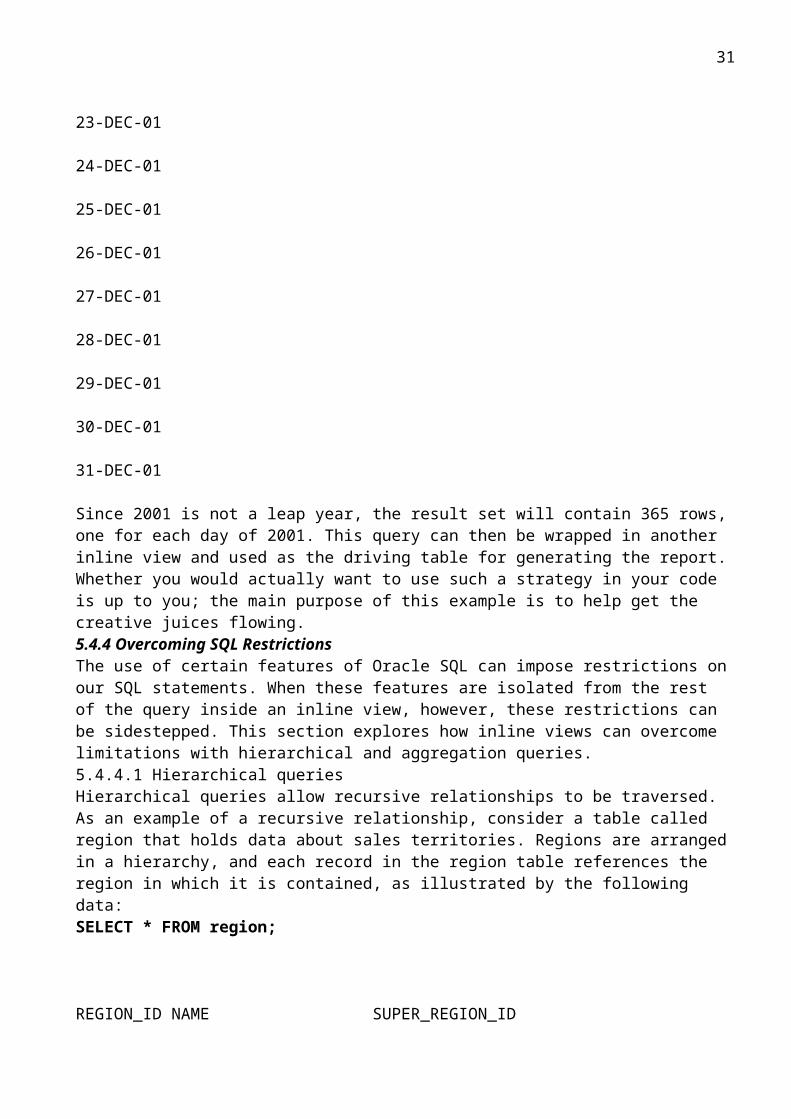
Since 2001 is not a leap year, the result set will contain 365 rows, one for each day of 2001. This query can then be wrapped in another inline view and used as the driving table for generating the report. Whether you would actually want to use such a strategy in your code is up to you; the main purpose of this example is to help get the creative juices flowing.5.4.4 Overcoming SQL RestrictionsThe use of certain features of Oracle SQL can impose restrictions on our SQL statements. When these features are isolated from the rest of the query inside an inline view, however, these restrictions can be sidestepped. This section explores how inline views can overcome limitations with hierarchical and aggregation queries.5.4.4.1 Hierarchical queriesHierarchical queries allow recursive relationships to be traversed. As an example of a recursive relationship, consider a table called region that holds data about sales territories. Regions are arranged in a hierarchy, and each record in the region table references the region in which it is contained, as illustrated by the following data:SELECT * FROM region;

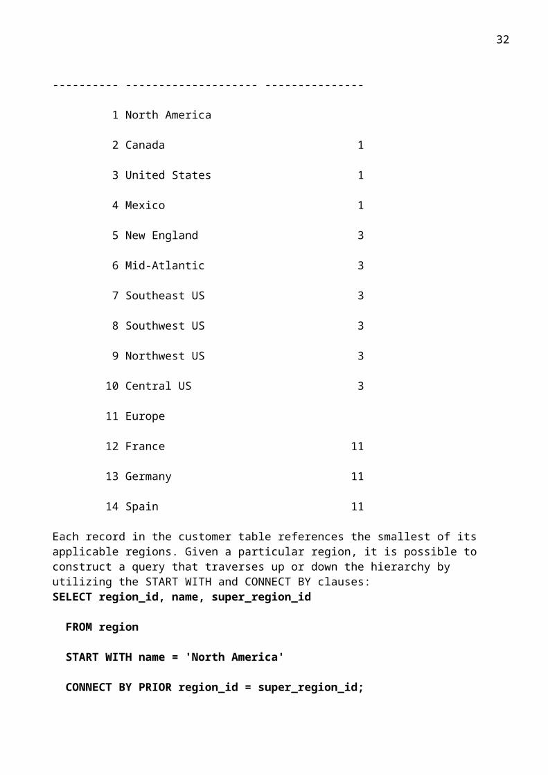
24

REGION_ID NAME SUPER_REGION_ID

---------- -------------------- ---------------

1 North America

2 Canada 1

3 United States 1

4 Mexico 1

5 New England 3

6 Mid-Atlantic 3

7 Southeast US 3

8 Southwest US 3

9 Northwest US 3

10 Central US 3

11 Europe

12 France 11

13 Germany 11

14 Spain 11

Each record in the customer table references the smallest of its applicable regions. Given a particular region, it is possible to construct a query that traverses up or down the hierarchy by utilizing the START WITH and CONNECT BY clauses:SELECT region_id, name, super_region_id

FROM region

START WITH name = 'North America'

CONNECT BY PRIOR region_id = super_region_id;

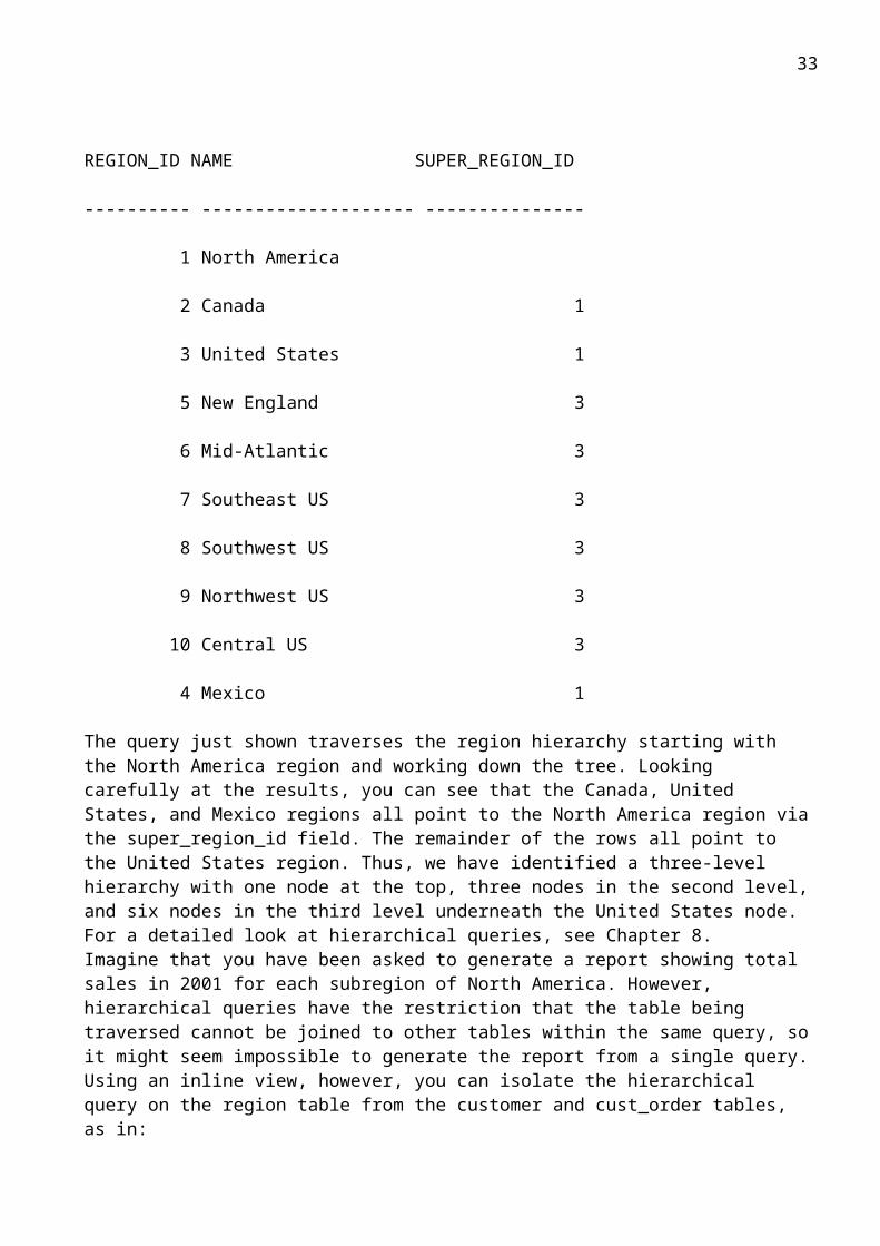
REGION_ID NAME SUPER_REGION_ID

---------- -------------------- ---------------

1 North America

25

2 Canada 1

3 United States 1

5 New England 3

6 Mid-Atlantic 3

7 Southeast US 3

8 Southwest US 3

9 Northwest US 3

10 Central US 3

4 Mexico 1

The query just shown traverses the region hierarchy starting with the North America region and working down the tree. Looking carefully at the results, you can see that the Canada, United States, and Mexico regions all point to the North America region via the super_region_id field. The remainder of the rows all point to the United States region. Thus, we have identified a three-level hierarchy with one node at the top, three nodes in the second level, and six nodes in the third level underneath the United States node. For a detailed look at hierarchical queries, see Chapter 8.Imagine that you have been asked to generate a report showing total sales in 2001 for each subregion of North America. However, hierarchical queries have the restriction that the table being traversed cannot be joined to other tables within the same query, so it might seem impossible to generate the report from a single query. Using an inline view, however, you can isolate the hierarchical query on the region table from the customer and cust_order tables, as in:SELECT na_regions.name region_name,

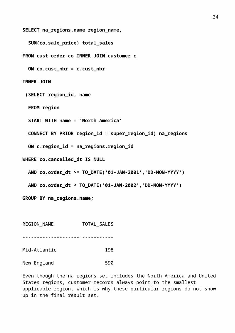
SUM(co.sale_price) total_sales

FROM cust_order co INNER JOIN customer c

ON co.cust_nbr = c.cust_nbr

INNER JOIN

(SELECT region_id, name

FROM region


CONNECT BY PRIOR region_id = super_region_id) na_regions

ON c.region_id = na_regions.region_id




26


GROUP BY na_regions.name;

REGION_NAME TOTAL_SALES

-------------------- -----------

Mid-Atlantic 198

New England 590

Even though the na_regions set includes the North America and United States regions, customer records always point to the smallest applicable region, which is why these particular regions do not show up in the final result set.By placing the hierarchical query within an inline view, you are able to temporarily flatten the region hierarchy to suit the purposes of the query, which allows you to bypass the restriction on hierarchical queries without resorting to splitting the logic into multiple pieces. The next section will demonstrate a similar strategy for working with aggregate queries.5.4.4.2 Aggregate queriesQueries that perform aggregations have the following restriction: all nonaggregate columns in the SELECT clause must be included in the GROUP BY clause. Consider the following query, which aggregates sales data by customer and salesperson, and then adds supporting data from the customer, region, employee, and department tables:SELECT c.name customer, r.name region,

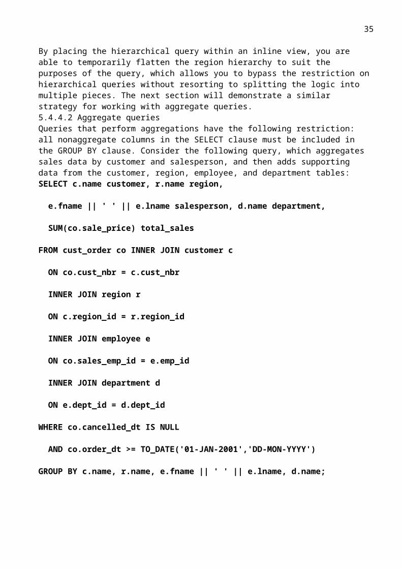
e.fname || ' ' || e.lname salesperson, d.name department,




INNER JOIN region r

ON c.region_id = r.region_id

INNER JOIN employee e

ON co.sales_emp_id = e.emp_id

INNER JOIN department d

ON e.dept_id = d.dept_id



27

GROUP BY c.name, r.name, e.fname || ' ' || e.lname, d.name;

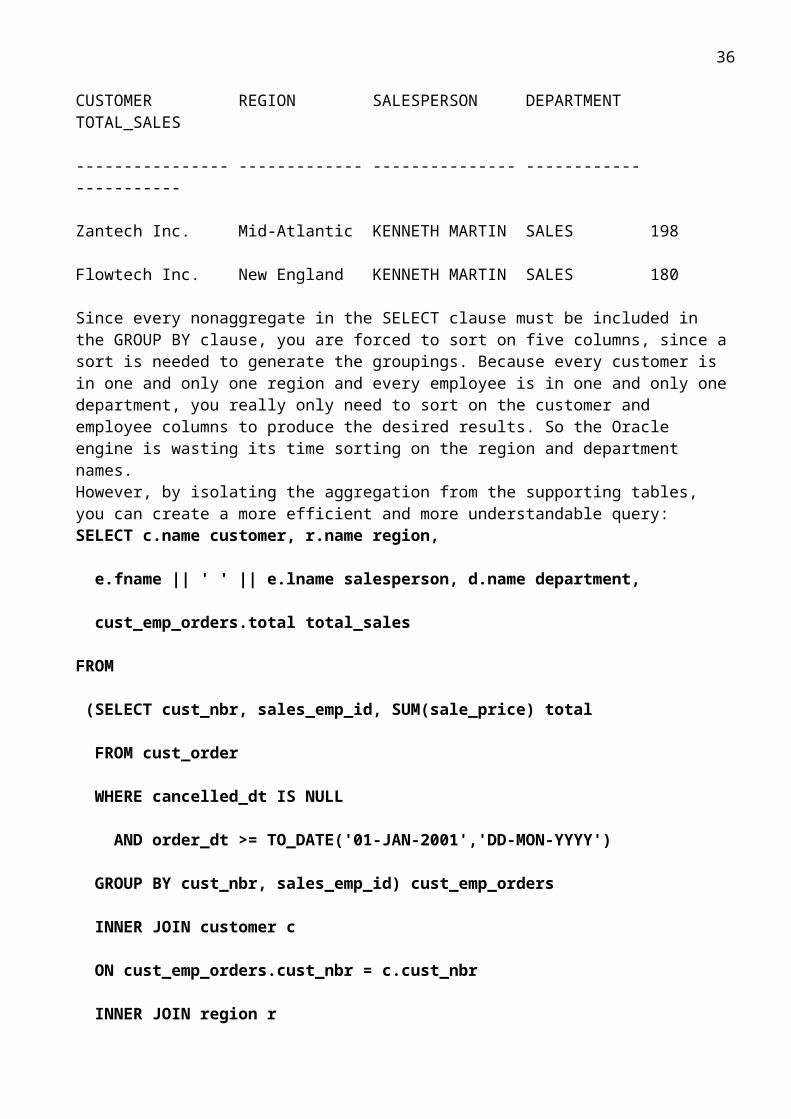
CUSTOMER REGION SALESPERSON DEPARTMENT TOTAL_SALES

---------------- ------------- --------------- ------------ -----------

Zantech Inc. Mid-Atlantic KENNETH MARTIN SALES 198

Flowtech Inc. New England KENNETH MARTIN SALES 180

Since every nonaggregate in the SELECT clause must be included in the GROUP BY clause, you are forced to sort on five columns, since a sort is needed to generate the groupings. Because every customer is in one and only one region and every employee is in one and only one department, you really only need to sort on the customer and employee columns to produce the desired results. So the Oracle engine is wasting its time sorting on the region and department names.However, by isolating the aggregation from the supporting tables, you can create a more efficient and more understandable query:SELECT c.name customer, r.name region,

e.fname || ' ' || e.lname salesperson, d.name department,

cust_emp_orders.total total_sales

FROM

(SELECT cust_nbr, sales_emp_id, SUM(sale_price) total

FROM cust_order

WHERE cancelled_dt IS NULL

AND order_dt >= TO_DATE('01-JAN-2001','DD-MON-YYYY')

GROUP BY cust_nbr, sales_emp_id) cust_emp_orders

INNER JOIN customer c

ON cust_emp_orders.cust_nbr = c.cust_nbr

INNER JOIN region r

ON c.region_id = r.region_id

INNER JOIN employee e

ON cust_emp_orders.sales_emp_id = e.emp_id

INNER JOIN department d

28

ON e.dept_id = d.dept_id;

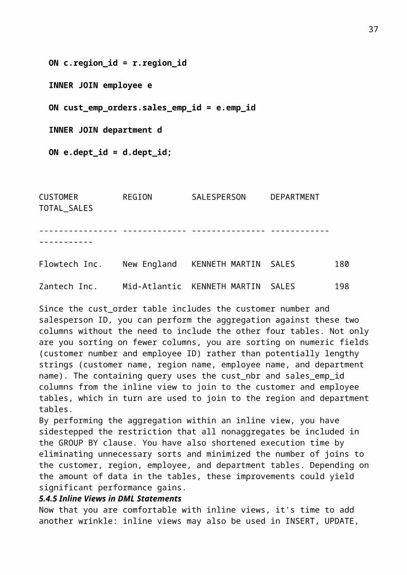
CUSTOMER REGION SALESPERSON DEPARTMENT TOTAL_SALES

---------------- ------------- --------------- ------------ -----------

Flowtech Inc. New England KENNETH MARTIN SALES 180

Zantech Inc. Mid-Atlantic KENNETH MARTIN SALES 198

Since the cust_order table includes the customer number and salesperson ID, you can perform the aggregation against these two columns without the need to include the other four tables. Not only are you sorting on fewer columns, you are sorting on numeric fields (customer number and employee ID) rather than potentially lengthy strings (customer name, region name, employee name, and department name). The containing query uses the cust_nbr and sales_emp_id columns from the inline view to join to the customer and employee tables, which in turn are used to join to the region and department tables.By performing the aggregation within an inline view, you have sidestepped the restriction that all nonaggregates be included in the GROUP BY clause. You have also shortened execution time by eliminating unnecessary sorts and minimized the number of joins to the customer, region, employee, and department tables. Depending on the amount of data in the tables, these improvements could yield significant performance gains.5.4.5 Inline Views in DML StatementsNow that you are comfortable with inline views, it's time to add another wrinkle: inline views may also be used in INSERT, UPDATE, and DELETE statements. In most cases, using an inline view in a DML statement improves readability but otherwise adds little value to statement execution. To illustrate, we'll begin with a fairly simple UPDATE statement and then show the equivalent statement using an inline view:UPDATE cust_order co

SET co.expected_ship_dt = co.expected_ship_dt + 7

WHERE co.cancelled_dt IS NULL AND co.ship_dt IS NULL

AND EXISTS (SELECT 1

FROM line_item li INNER JOIN part p


WHERE li.order_nbr = co.order_nbr

AND p.inventory_qty = 0);

This statement uses an EXISTS condition to locate orders that include out-of-stock parts. The next version uses an inline view called suspended_orders to identify the same set of orders:UPDATE (SELECT co.expected_ship_dt exp_ship_dt

FROM cust_order co

29


AND EXISTS (SELECT 1

FROM line_item li INNER JOIN part p


WHERE li.order_nbr = co.order_nbr

AND p.inventory_qty = 0)) suspended_orders

SET suspended_orders.exp_ship_dt = suspended_orders.exp_ship_dt + 7;

In the first statement, the WHERE clause of the UPDATE statement determines the set of rows to be updated, whereas in the second statement, the result set returned by the SELECT statement determines the target rows. Otherwise, the two statements are identical. For the inline view to add extra value to the statement, it must be able to do something that the simple update statement cannot do: join multiple tables. The following version attempts to do just that by replacing the subquery with a three-table join:UPDATE (SELECT co.expected_ship_dt exp_ship_dt


ON co.order_nbr = li.order_nbr

INNER JOIN part p



AND p.inventory_qty = 0) suspended_orders

SET suspended_orders.exp_ship_dt = suspended_orders.exp_ship_dt + 7;

However, statement execution results in the following error:ORA-01779: cannot modify a column which maps to a non key-preserved table

As is often the case in life, we can't get something for nothing. To take advantage of the ability to join multiple tables within a DML statement, we must abide by the following rules: Only one of the joined tables in an inline view may be modified by the containing DML statement. To be modifiable, the target table's key must be preserved in the result set of the inline view.Although the previous UPDATE statement attempts to modify only one table (cust_order), that table's key (order_nbr) is not preserved in the result set, since an order has multiple line items. In other words, rows in the result set generated by the three-table join cannot be uniquely identified using just the order_nbr field, so it is not possible to update the cust_order table via this particular three-table join. However, it is possible to update or delete from the line_item table using the same join, since the key of the line_item table matches the key of the result set returned from the inline view (order_nbr and part_nbr). The next statement deletes rows from the line_item table using an inline view nearly identical to the one that failed for the previous UPDATE attempt:DELETE FROM (SELECT li.order_nbr order_nbr, li.part_nbr part_nbr

30


ON co.order_nbr = li.order_nbr

INNER JOIN part p



AND p.inventory_qty = 0) suspended_orders;

The column(s) referenced in the SELECT clause of the inline view are actually irrelevant. Since the line_item table is the only key-preserved table of the three tables listed in the FROM clause, this is the table on which the DELETE statement operates. Although utilizing an inline view in a DELETE statement can be more efficient, it's somewhat disturbing that it is not immediately obvious which table is the focus of the DELETE statement. A reasonable convention when writing such statements would be to always select the key columns from the target table.5.4.6 Restricting Access Using WITH CHECK OPTIONAnother way in which inline views can add value to DML statements is by restricting both the rows and columns that may be modified. For example, most companies only allow members of Human Resources to see or modify salary information. By restricting the columns visible to a DML statement, we can effectively hide the salary column:UPDATE (SELECT emp_id, fname, lname, dept_id, manager_emp_id

FROM employee) emp

SET emp.manager_emp_id = 11

WHERE emp.dept_id = 4;

Although this statement executes cleanly, attempting to add the salary column to the SET clause would yield the following error:UPDATE (SELECT emp_id, fname, lname, dept_id, manager_emp_id

FROM employee) emp

SET emp.manager_emp_id = 11, emp.salary = 1000000000


ORA-00904: "EMP"."SALARY": invalid identifier

Of course, the person writing the UPDATE statement has full access to the table; the intent here is to protect against unauthorized modifications by the users. This might prove useful in an n-tier environment, where the interface layer interacts with a business-logic layer.Although this mechanism is useful for restricting access to particular columns, it does not limit access to particular rows in the target table. To restrict the rows that may be modified using a DML statement, you can add a WHERE clause to the inline view and specify WITH CHECK OPTION. For example,

31

you may want to restrict the users from modifying data for any employee in the Accounting department:UPDATE (SELECT emp_id, fname, lname, dept_id, manager_emp_id

FROM employee

WHERE dept_id !=

(SELECT dept_id FROM department WHERE name = 'ACCOUNTING')

WITH CHECK OPTION) emp

SET emp.manager_emp_id = 7698


The addition of WITH CHECK OPTION to the inline view protects against any data modifications that would not be visible via the inline view. For example, attempting to modify an employee's department assignment from Sales to Accounting would generate an error, since the data would no longer be visible via the inline view:UPDATE (SELECT emp_id, fname, lname, dept_id, manager_emp_id

FROM employee

WHERE dept_id !=

(SELECT dept_id FROM department WHERE name = 'ACCOUNTING')

WITH CHECK OPTION) emp

SET dept_id = (SELECT dept_id FROM department WHERE name = 'ACCOUNTING')

WHERE emp_id = 7900;

ORA-01402: view WITH CHECK OPTION where-clause

violation

5.4.7 Global Inline ViewsEarlier in the chapter, you saw how the WITH clause can be used to allow the same subquery to be referenced multiple times within the same query. Another way to utilize the WITH clause is as an inline view with global scope. To illustrate, we will rework one of the previous inline view examples to show how the subquery can be moved from the FROM clause to the WITH clause. Here's the original example, which comes from Section 5.4.4.1:SELECT na_regions.name region_name,


mk:@MSITStore:G:%5C_____Gramatas_un_pasutisana%5CSQL%5CPamati%5C_A_Beaulieu_Mastering_Oracle_SQL_2004.chm::/0596006322/mastorasql2-CHP-5-SECT-4.html#mastorasql2-CHP-5-SECT-4.4.1

32



INNER JOIN

(SELECT region_id, name

FROM region


CONNECT BY PRIOR region_id = super_region_id) na_regions







-------------------- -----------

Mid-Atlantic 198

New England 590

Here's the same query with the na_regions subquery moved to the WITH clause:WITH na_regions AS (SELECT region_id, name

FROM region


CONNECT BY PRIOR region_id = super_region_id)

SELECT na_regions.name region_name,




INNER JOIN na_regions

33







-------------------- -----------

Mid-Atlantic 198

New England 590

Note that the FROM clause must include the inline view alias for you to reference the inline view's columns in the SELECT, WHERE, GROUP BY, or ORDER BY clauses.To show how the na_regions subquery has global scope, the join between the na_regions inline view and the customer table has been moved to another inline view (called cust) in the FROM clause:WITH na_regions AS (SELECT region_id, name

FROM region


CONNECT BY PRIOR region_id = super_region_id)

SELECT cust.region_name region_name,



(SELECT c.cust_nbr cust_nbr, na_regions.name region_name

FROM customer c INNER JOIN na_regions

ON c.region_id = na_regions.region_id) cust

ON co.cust_nbr = cust.cust_nbr




34

GROUP BY cust.region_name;


-------------------- -----------

Mid-Atlantic 198

New England 590

Earlier in this section, we stated that inline views "are always executed prior to the containing query and, thus, may not reference columns from other tables or inline views from the same query." Using the WITH clause, however, you are able to break this rule, since the na_regions inline view is visible everywhere within the query. This makes the na_regions inline view act more like a temporary table than a true inline view.5.5 Subquery Case Study: The Top N PerformersCertain queries that are easily described in English have traditionally been difficult to formulate in SQL. One common example is the "Find the top five salespeople" query. The complexity stems from the fact that data from a table must first be aggregated, and then the aggregated values must be sorted and compared to one another to identify the top or bottom performers. In this section, you will see how subqueries may be used to answer such questions. At the end of the section, we introduce ranking functions, a feature of Oracle SQL that was specifically designed for these types of queries.5.5.1 A Look at the DataConsider the problem of finding the top five salespeople. Let's assume that we are basing our evaluation on the amount of revenue each salesperson brought in during the previous year. The first task, then, would be to sum the dollar amount of all orders booked by each salesperson during the year in question. To do so, we will dip into our data warehouse, in which orders have been aggregated by salesperson, year, month, customer, and region. The following query generates total sales per salesperson for the year 2001:SELECT s.name employee, SUM(o.tot_sales) total_sales

FROM orders o INNER JOIN salesperson s

ON o.salesperson_id = s.salesperson_id

WHERE o.year = 2001

GROUP BY s.name

ORDER BY 2 DESC;

EMPLOYEE TOTAL_SALES

------------------------------ -----------

Jeff Blake 1927580

35

Sam Houseman 1814327

Mark Russell 1784596

John Boorman 1768813

Carl Isaacs 1761814

Tim McGowan 1761814

Chris Anderson 1757883

Bill Evans 1737093

Jim Fletcher 1735575

Mary Dunn 1723305

Dave Jacobs 1710831

Chuck Thomas 1695124

Greg Powers 1688252

Don Walters 1672522

Alex Fox 1645204

Barbara King 1625456

Lynn Nichols 1542152

Karen Young 1516776

Bob Grossman 1501039

Eric Iverson 1468316

Tom Freeman 1461898

Andy Levitz 1458053

Laura Peters 1443837

Susan Jones 1392648

It appears that Isaacs and McGowan have tied for fifth place, which, as you will see, adds an interesting wrinkle to the problem.5.5.2 Your AssignmentIt seems that the boss was so tickled with this year's sales that she has asked you, the IT manager, to see that each of the top five salespeople receive a bonus equal to 1% of their yearly sales. No problem,

36

you say. You quickly throw together the following report using your favorite feature, the inline view, and send it off to the boss:SELECT s.name employee, top5_emp_orders.tot_sales total_sales,

ROUND(top5_emp_orders.tot_sales * 0.01) bonus

FROM

(SELECT all_emp_orders.salesperson_id emp_id,

all_emp_orders.tot_sales tot_sales

FROM

(SELECT salesperson_id, SUM(tot_sales) tot_sales

FROM orders

WHERE year = 2001

GROUP BY salesperson_id

ORDER BY 2 DESC

) all_emp_orders

WHERE ROWNUM <= 5

) top5_emp_orders INNER JOIN salesperson s

ON top5_emp_orders.emp_id = s.salesperson_id

ORDER BY 2 DESC;

EMPLOYEE TOTAL_SALES BONUS

------------------------------ ----------- ----------

Jeff Blake 1927580 19276

Sam Houseman 1814327 18143

Mark Russell 1784596 17846

John Boorman 1768813 17688

Tim McGowan 1761814 17618

The howl emitted by Isaacs can be heard for five square blocks. The boss, looking a bit harried, asks you to take another stab at it. Upon reviewing your query, the problem becomes immediately evident;

37

the inline view aggregates the sales data and sorts the results, and the containing query grabs the first five sorted rows and discards the rest. Although it could easily have been McGowan, since there is no second sort column, Isaacs was arbitrarily omitted from the result set.5.5.3 Second AttemptYou console yourself with the fact that you gave the boss exactly what she asked for: the top five salespeople. However, you realize that part of your job as IT manager is to give people what they need, not necessarily what they ask for, so you rephrase the boss's request as follows: give a bonus to all salespeople whose total sales ranked in the top five last year. This will require two steps: find the fifth highest sales total last year, and then find all salespeople whose total sales meet or exceed that figure. You write a new query as follows:SELECT s.name employee, top5_emp_orders.tot_sales total_sales,


FROM salesperson s INNER JOIN

(SELECT salesperson_id, SUM(tot_sales) tot_sales

FROM orders

WHERE year = 2001


HAVING SUM(tot_sales) IN

(SELECT all_emp_orders.tot_sales

FROM

(SELECT SUM(tot_sales) tot_sales

FROM orders

WHERE year = 2001


ORDER BY 1 DESC

) all_emp_orders

WHERE ROWNUM <= 5)

) top5_emp_orders

ON top5_emp_orders.salesperson_id = s.salesperson_id

ORDER BY 2 DESC;

38


------------------------------ ----------- ----------

Jeff Blake 1927580 19276





Carl Isaacs 1761814 17618

Thus, there are actually six top five salespeople. The main difference between your first attempt and the second is the addition of the HAVING clause in the inline view. The subquery in the HAVING clause returns the five highest sales totals, and the inline view then returns all salespeople (potentially more than five) whose total sales exist in the set returned by the subquery.Although you are confident in your latest results, there are several aspects of the query that bother you: The aggregation of sales data is performed twice. The query will never contend for Most Elegant Query of the Year. You could've sworn you read about some sort of feature just for handling these types of queries . . .In fact, there is a feature, an analytic SQL feature, for performing ranking queries that became available with Oracle8i. That feature is the RANK function.5.5.4 Final AnswerThe RANK function is specifically designed to help you write queries to answer questions like the one posed in this case study. Part of a set of analytic functions (all of which will be explored in Chapter 14), the RANK function may be used to assign a ranking to each element of a set. The RANK function understands that there may be ties in the set of values being ranked and leaves gaps in the ranking to compensate. The following query illustrates how rankings would be assigned to the entire set of salespeople; notice how the RANK function leaves a gap between the fifth and seventh rankings to compensate for the fact that two rows share the fifth spot in the ranking:SELECT salesperson_id, SUM(tot_sales) tot_sales,

RANK( ) OVER (ORDER BY SUM(tot_sales) DESC) sales_rank

FROM orders

WHERE year = 2001

GROUP BY salesperson_id;

SALESPERSON_ID TOT_SALES SALES_RANK

-------------- ---------- ----------

1 1927580 1



39

14 1814327 2

24 1784596 3

8 1768813 4

15 1761814 5

16 1761814 5

20 1757883 7

11 1737093 8

9 1735575 9

10 1723305 10

17 1710831 11

4 1695124 12

5 1688252 13

12 1672522 14

19 1645204 15

18 1625456 16

21 1542152 17

13 1516776 18

3 1501039 19

22 1468316 20

2 1461898 21

7 1458053 22

23 1443837 23

6 1392648 24

Leaving gaps in the rankings whenever ties are encountered is critical for properly handling these types of queries. (If you do not wish to have gaps in the ranking, you can use the DENSE_RANK function intead.) Table 5-1 shows the number of rows that would be returned for this data set for various top-N queries.

mk:@MSITStore:G:%5C_____Gramatas_un_pasutisana%5CSQL%5CPamati%5C_A_Beaulieu_Mastering_Oracle_SQL_2004.chm::/0596006322/mastorasql2-CHP-5-SECT-5.html#mastorasql2-CHP-5-TABLE-1

40

Table 5-1. Rows returned for N = {1,2,3,...,9}

Top-N salespeople Rows returned

1 1

2 2

3 3

4 4

5 6

6 6

7 7

8 8

9 9

As you can see, the result sets would be identical for both the "top five" and "top six" versions of this query for this particular data set.By wrapping the previous RANK query in an inline view, you can retrieve the salespeople with a ranking of five or less and join the results to the salesperson table to generate the final result set:SELECT s.name employee, top5_emp_orders.tot_sales total_sales,


FROM

(SELECT all_emp_orders.salesperson_id emp_id,

all_emp_orders.tot_sales tot_sales

FROM

(SELECT salesperson_id, SUM(tot_sales) tot_sales,

RANK( ) OVER (ORDER BY SUM(tot_sales) DESC) sales_rank

FROM orders

WHERE year = 2001


) all_emp_orders

WHERE all_emp_orders.sales_rank <= 5

) top5_emp_orders INNER JOIN salesperson s

ON top5_emp_orders.emp_id = s.salesperson_id

41

ORDER BY 2 DESC;


------------------------------ ----------- ----------

Jeff Blake 1927580 19276





Carl Isaacs 1761814 17618

If this query looks familiar, that's because it's almost identical to the first attempt, except that the RANK function is used instead of the pseudocolumn ROWNUM to determine where to draw the line between the top five salespeople and the rest of the pack.Now that you are happy with your query and confident in your results, you show your findings to your boss. "Nice work," she says. "Why don't you give yourself a bonus as well? In fact, you can have Isaacs's bonus, since he quit this morning." Salespeople can be so touchy.

Documents

5.2 Noncorrelated Subqueries - … · Web view05-10-2017 · FORD. As this query ... Whether you would actually want to use such a strategy in your code is up to you; ... 5.5 Subquery