5.1 A One-dimensional Higgs Modelsbhepnt.physics.sunysb.edu/~rijssenbeek/PHY557_F08_L10.pdf5 The Higgs Mechanism ... of a boson field with an odd shape, i.e. a non-zero expectation

Part III The Field Theories 112 12/15/2008

5 The Higgs Mechanism The Higgs Mechanism, first invented by Peter Higgs, was used by Veltman and ‘t Hooft and others to lend mass to the gauge vector bosons of the weak interactions. The gauge fields (vector bosons) that are introduced to make the local gauge invariance of the particle field in the Lagrangian possible must necessarily be massless. Mass terms for a vector boson, like m2AμAμ, do not stay invariant under the transforma-tion of Aμ→Aμ’=Aμ−∂μα/q. For the photon field this is perfectly fine, but is clearly not acceptable for the massive weak vector bosons. The introduction of a complex scalar Higgs field into the Lagrangian, with a non-zero expectation value (a non-zero vacuum energy density) turns the initially massless gauge bosons into massive bosons, while one of the two Higgs field components disappears. In addition to “giving mass” to the weak vector bosons, W± and Z0, the Higgs field also couples to the fermion fields in the Standard Model Lagrangian, and by its couplings gives them mass as well. We’ll discuss the Higgs mechanism first, using first a one-dimensional and then a two-dimensional toy model (historically named the sigma-model).

5.1 A One-dimensional Higgs Model Consider the Lagrangian density for a real scalar (spin 0) Klein-Gordon field φ, see equation (III.16):

2 2 2 41 1 1( ) ( ) ( ), with ( )2 2 4

L T V V Vμμφ φ φ φ μ φ λ φ= − = ∂ ∂ − = + (III.149)

The potential V(φ) is a function of the “generalized coordinate” φ(x), and has a parabolic shape around the minimum at φ(x)=0. This Lagran-gian exhibits a simple reflection symmetry under φ → φ’ = −φ around the minimum. For small deviations from the minimum |φ|<<1, V(φ) ≈ ½μ2φ2, and:

( )2 2 2 2K-G

equation1 1( ) ( ) 0 (Klein-Gordon equation)2 2

E LL T V μ

μφ φ μ φ μ φ−

= − = ∂ ∂ − ⇒ ∂ + = (III.150)

which is the Lagrangian for a massive Klein-Gordon field φ; note the relative minus sign between kinetic and mass terms in L. Note that the mass term is intimately connected to a positive parabolic shape of the potential V(φ’) around the origin of the field; i.e. no such parabola then no mass term! So far, nothing is new... Now, consider what happens if we change the potential to V(φ) = −½μ2φ2 + ¼ λ2φ4. This potential has a “bottoms-up” shape. The “point” φ=0 has become a local maximum, with two degenerate minima on either side of the origin at φ = ±|μ/λ|. There is no obvious mass term for small φ. The Lagrangian exhibits the reflection symmetry around the origin at φ=0. However, the vacuum state, i.e. the lowest energy state, is no longer at φ=0. The true vacuum state must be at one of the two minima, say the minimum at φ = v ≡ +|μ/λ|. We can now rewrite the Lagrangian in terms of small deviations φ’ with respect to this minimum v; thus φ ≡ v + φ’:


( )( )2 2 2 4 2 2 2 4

22 2 2 2 2 4 4 3 3 2 2

2

22 2

2

1 1 1 1 1 1( ) ( ) ( ' ) ( ' ) ( ' ) ( ' )2 2 4 2 2 41 1 1 1( ') ( ') ' ' ( ' 4 ' 4 ' 6 ' )2 2 2 4

1 1( ') ( ') '2 4mass termKinetic Energy term

L v v v v

v v v v v vv

v

μ μμ μ

μμ

μμ

φ φ μ φ λ φ φ φ μ φ λ φ

μφ φ μ φ μ φ μ φ φ φ φ

μφ φ μ φ

= ∂ ∂ + − = ∂ + ∂ + + + − + =

= ∂ ∂ + + + − + + + + =

= ∂ ∂ + − − 4 3 2 21( ' 4 ' )4

constanthigher order terms

v vφ φ μ+ +

(III.151)

In summary: we obtain a kinetic Klein-Gordon term (the derivative squared) for field φ’, a proper mass term (the second term) for a particle of mass m=μ√2, and triple and quartic vertex coupling terms of the field φ’ (the third term in brackets). The last term is a constant and can be ignored (it doesn’t lead to any term in the Euler-Lagrange equation of motion). We have regained a mass term for the field when expanding the field about its vacuum value (local minimum). The original reflection symmetry, when expressed in the field φ’, disappears and is now hidden; it should reappear if we were to re-write the Lagrangian in terms of the original field φ. A mechanical analogy can be made: consider a plastic ruler held vertical at the ends. A vertical force is applied straight down at the top of the ruler. For a small enough vertical force, the ruler will re-main straight, and tapping the ruler sideways at the middle may induce small oscillations, see the left figure. The situation is perfectly left-right symmetric. However, for a somewhat larger vertical force downwards, the right figure, the rule will find a new equilibrium position when it is bent either to the left or to the right. The system’s symmetry is no longer apparent. Small oscillations may be induced around the new energy minimum. Only much larger oscillations, caused by a substantial sideward tap, will pass through the local maximum in the center, and are again symmetric around the vertical position.

5.2 A QED Model with a Complex Higgs Field Let us now consider a slightly more complicated Lagrangian, which will exhibit a local (and continuous) gauge invariance. We will take Quantum Electro-Dynamics as the example of choice. In addition to the Electromagnetic photon field kinetic term ¼FμνFμν, we will again add a potential with local maximum near the origin. This time we will take a complex scalar field φ as in section 2.4 above. This φ may be de-

F F

Re(φ)

Im(φ)

V(φ)

v

v

φ φ’

Re(φ)

Im(φ)

ζ

η

valley of minima


composed into two independent fields φ1 and φ2 of equal mass, e.g. by defining φ =(φ1+iφ2)/√2; in fact it is a handy way of keeping track of the two equal-mass fields. In the following it will be shown that the coupling of the field φ with the photon Aμ leads to an effective mass term for the photon. In addi-tion, of the two independent components of φ, only one remains; the other field has been “eaten” by the photon, which thereby gained weight! Note, that this is all accomplished without breaking gauge invariance! Consider the Lagrangian:

( )2 41 1* 2 22 4

1 1( ) ( ) ( )2 4

( )QED QEDL T T V D D F F

V

μ μνφ μ μνφ φ φ μ φ λ φ

φ

= + − = − − − + (III.152)

where φ is a complex scalar field, and where: ,D iqA F A Aμ μ μ μν μ ν ν μ≡ ∂ + ≡ ∂ − ∂ (III.153) and with φ(x) and Aμ(x) transforming under local phase/gauge transformations as:

( )( ) '( ) ( )

( ) '( ) ( ) ( )

i xx x e xA x A x A x x q

α

μ μ μ μφ φ φ

α⎧ =⎫ →⎬ ⎨ = − ∂⎭ ⎩

(III.154)

It is clear that the above Lagrangian is invariant under such transformations by construction (see also section 2.5); it contains a massless photon. Now observe what happens when we consider small deviations around the true minimum. The locus of minima forms a full circle in the complex plane of the complex generalized coordinate φ(x), with a radius v = |μ/λ|: the dashed red circle in the figure. The minima are degen-erate: oscillations along the valley bottom cost no energy and we expect those to be massless. In contrast, oscillations perpendicular to the valley floor are experiencing a parabolic potential and will lead to a mass term. As before, we will pick a convenient vacuum expectation value, φ = v (real), and consider small oscillations φ’(x) = φ(x) − v around this vac-uum. The complex field φ’(x) consists of two independent real fields, η(x) and ζ(x), so that φ’(x) ≡ [η(x) + iζ(x)]/√2. For small |φ’(x)|<<v, we may write:

( ) ( ) ( )/1 1( ) '( ) ( ) ( ) ( ) for ( ) , ( )2 2

i x vx v x v x i x v x e x x vζφ φ η ζ η η ζ≡ + = + + ≈ + << (III.155)

Note that indeed the (phase) angle of φ is ≈ζ/v. Substituting expression (III.155) into the Lagrangian, we expect to see terms appearing in the new fields η(x) and ζ(x). However, the field ζ(x) enters only as a phase factor exp(iζ(x)/v). Because the Lagrangian is explicitly invariant under local phase rotations, we may actually use the local gauge freedom to rotate the phase factor away by the gauge transformation:

( ) ( )/ / ( )/1 1" ( ) ( )2 2

"( ) ( ) ( )

i v i v i x ve e v x e v xA

A x A x x qv

ζ ζ ζ

μμ μ μ

φ φ η ηφ

ζ

− −⎧ ≡ ≈ + = +⎪⎫ →⎬ ⎨⎭ ⎪ = + ∂⎩

(III.156)


Thus the ζ(x) field will be completely absent from the Lagrangian! Note that the choice of minimum (vacuum) φ0 = v = real, is not so spe-cial; after all any other vacuum expectation value can be reached simply by making an appropriate phase rotation in the weak isospin space. Let us see the other consequences that result from the change in perspective – looking at the field φ as deviations φ” from the minimum v. Without loss of generality we may thus make the replacement φ → v+η(x):

( )( )( )( ) ( ) ( )

( )( )

( ) ( )( )

2 41 1 1 1* 2 22 2 4 4

2 2 41 1 1 12 22 2 4 4

3 4 221 12 222 4

3 42 21 1 2 2 2 22 2

( " ") ( " ") " " " "

( ) ( ) ( )

" ( )4 4

" "4

v

L D D F F

iq A qv v x v x v x F F

viqA v x F Fv v

q A A vv v

μ μνμ μν

λ μμν

μ μ μ μν

μνμ μ μν

μμ μ

φ φ μ φ λ φ

ζ η μ η λ η

η ηη μ η

η ηη η μ η μ

=

= − − + − =

= ∂ + + ∂ + + + − + − =

⎛ ⎞= ∂ + + − + + − − =⎜ ⎟

⎝ ⎠

= ∂ + + − − +

( ) ( )

21

2 4

1 1 1 12 2 2 2 2 2 2 2 3 4 22 4 2 2

K.E. of Photon Photon mass Triple and Quartic -Photon couplingsK-G equation for massive self coupl

4

( )( ) 2 " " " " " " 4/ /

v F F

F F q v A A q A A q v A A v v

μνμν

μ μν μ μ μμ μν μ μ μ

ηη η

η η μ η η η μ η η

⎛ ⎞− − =⎜ ⎟

⎝ ⎠

= ∂ ∂ − − + + + − +ings

(III.157)

In conclusion: we find that if we break the symmetry (by considering the field φ with respect to a chosen minimum) in a theory that exhibits local gauge invariance, the initially massless gauge field (the field Aμ(x)) acquires a mass. In return, one of the scalar fields disappears (the tangential field ζ(x)), leaving a single real, massive, scalar (Higgs) radial field η(x):

2-field, (real), mass: 2-field disappers; is 'rotated away'

-field, acquires mass: A qvμ

η μζ (III.158)


6 Symmetries of the Standard Model: U(1), SU(2), SU(3) We’ve now constructed a powerful toolset: we know how to describe free elementary particles: bosons using the Klein-Gordon Lagrangian; and fermions using the Dirac Lagrangian. We introduce interactions by the use of the gauge principle: requiring invariance of the Lagran-gian under local phase/gauge transformations of the particle fields, we are led to introduce ‘compensating gauge fields’ of the proper form. The gauge fields have to be massless in order to preserve gauge invariance, which is clearly a problem when considering weak interactions where the gauge bosons are massive. However, we can overcome this problem by invoking the Higgs mechanism: postulating the existence of a boson field with an odd shape, i.e. a non-zero expectation value, and by re-expressing the Higgs field with respect to a true minimum (vacuum), we break the manifest symmetry of the Lagrangian, but reap great benefits as well: the gauge boson acquires mass, just what we need for the weak gauge bosons. A final benefit from the use of a theory with local gauge invariance is that such theories are inherently self-consistent when higher-order diagrams are considered. Very elegant cancellations between diagrams occur, which cure divergencies that would otherwise make the theory meaningless. We label the gauge symmetry by their group structure. The simplest gauge transformation is the multiplication of the field by a phase factor function: exp{iα (x)} ≡ 1 + iα + (iα)2/2! + (iα)3/3! + ... , which is the (infinite) group of complex functions that have modulus 1. The group operation is multiplication (addition of the phase angles), and the unit element is exp{0} = 1. The group’s elements are clearly unitary: [exp{iα(x)}]† = exp{−iα(x)} = [exp{iα(x)}]−1. The official name of the group is “unitary group of dimension one”: U(1) for short. More complicated gauge groups are formed by bringing in matrices: e.g. the 2×2 Pauli matrices exp{i½σ⋅β(x)} ≡ 12 + i½σ⋅β + (i½σ⋅β)2/2! + (i½σ⋅β)3/3! + ... . This group is again an infinite group of complex operator functions that have determinant 1 and are unitary. They are uni-tary because the Pauli matrices are Hermitian (and so is iσ⋅β); because the Pauli matrices are traceless we also find that det[exp{i½σ⋅β}] = exp{Tr[i½σ⋅β]} = exp{0} = 1. This group’s name is special unitary group of dimension 2, SU(2). Its generators are the Pauli Matrices, be-cause any member of the group can be formed by appropriate combinations of the three Pauli matrices.

6.1 The SU(2)L of Weak Isospin The basic particle for the weak interactions is the doublet consisting of the (electron) neutrino and the electron. The weak interaction proc-esses that we have seen – muon decay, or neutron decay – proceed by coupling of the W vector boson to the left-handed neutrino-electron or up-down quark doublets:

* *

* ** *

* *

,

,,

,

e

ee

e

W W e

n p W W ed u W W e

W W e

μμ ν ν

νν

π ν

− − − −

− − −− − −

− − − −

→ + → +

⎫→ + → + ⎪ = → + → +⎬→ → + ⎪⎭

(III.159)

where the W−* is a virtual W−, which means that its mass (= length of its fourvector) is not its nominal “on-shell” mass of 80.41 GeV. As far as we can tell, the weak interaction treats left-handed neutrinos and left-handed electrons exactly the same: the weak interaction does not care about the electric charge difference, or about the mass difference between the two. The left-handed up-quark and down-quark also form a weak doublet: they turn into one another by the emission or absorption of a W boson, just like the electron and the electron-neutrino.


This apparent invariance under “rotations of the doublet” (the weak left-handed doublet) is an exact analog of the spin formalism of spin-½ electrons, and the strong isospin considered in the beginning. Thus, we will assign the left-handed neutrino a weak isospin z-component of +½, and the electron −½: 1 1 1 1(3) (3)

2 2 2 2, , , , ,eW W W We I I I Iν− = = − = = + (III.160) We will require the weak Lagrangian to be invariant for gauge transformations of the SU(2) of weak isospin (rotations in the weak isospin space):

( )/2 3 1 2 3 1 22 2

1 2 3 1 2 3

' ( ) ( )exp exp( ) ( )'i ii x ee e e e

L L L L

i i i i i ie i i i i i i ee e e eνν ν ν νβ β β β β β

β β β β β β⋅

−− − − −⎧ − ⎫ ⎧ − ⎫⎛ ⎞⎛ ⎞ ⎛ ⎞ ⎛ ⎞ ⎛ ⎞⎛ ⎞ ⎛ ⎞→ = = =⎨ ⎬ ⎨ ⎬⎜ ⎟ ⎜ ⎟⎜ ⎟ ⎜ ⎟ ⎜ ⎟ ⎜ ⎟ ⎜ ⎟+ − + −⎝ ⎠ ⎝ ⎠⎝ ⎠ ⎝ ⎠ ⎝ ⎠ ⎝ ⎠ ⎝ ⎠⎩ ⎭ ⎩ ⎭

σ β L

L

PP

(III.161)

with PL ≡ ½(1−γ5) acting on the Dirac spinors for the neutrino and for the electron as before. For the SU(2) invariance to be established, we need to replace the regular derivative ∂μ everywhere by the SU(2) covariant derivative Dμ, with Dμ ≡ ∂μ + ½igσ⋅bμ, and g an arbitrary coupling constant. The transformation of the gauge fields bμ(x) is closely linked to the three fields β(x), because its transformation needs to cancel terms arising from derivatives of β(x):

1 ( )1 1 2' ( ) , with

i xiU U U U U eg

μ μ μ ⋅− −= + ∂ ≡βσ

b b (III.162)

We can explore this a bit, and use the infinitesimal form to ease the calculus, i.e. we will take |β(x)|<<1. We expect bμ’ = bμ + δbμ, with δbμ small in the infinitesimal approximation. Then, requiring that Dμψ transform like ψ itself under the transformation:

( )

12

12

12

1 1 12 2 2

1 12 2

( ) ' ( ), with

evaluating the left-hand and right-hand sides separately:

LHS: ( ) ' ' ' ' ' 1

( ')

i

i

D e D D ig

D D ig e ig i

ig i

μ μ μ μ μ

μ μ μ μ μ μ

μ μ

ψ ψ

ψ ψ ψ ψ

ψ ψ

⋅

⋅

= ≡ ∂ + ⋅

⇓

⎡ ⎤ ⎡ ⎤= = ∂ + ⋅ ≈ ∂ + ⋅ + ⋅ =⎣ ⎦ ⎣ ⎦

= ∂ + ⋅ +

σ β

σ β

σ b

σ b σ b σ β

σ b ( )( ) { }

( ) ( )12

1 12 4

1 1 1 12 2 2 4

1 1 12 2 2

1 1 12 2 4

( ) ( ) ( ')( )

( ') ( ) ( ) ( )( ) ( )( )

RHS: ( ) 1 1

( ) ( ) (

i

i g

ig i i g

e D i D i ig

ig i g

μ μ μ

μ μ μ μ μ μ

μ μ μ μ

μ μ μ

ψ ψ ψ

ψ ψ ψ ψ δ ψ

ψ ψ ψ

ψ ψ ψ

⋅

⋅ ∂ + ⋅ ∂ − ⋅ ⋅ =

= ∂ + ⋅ + ⋅ ∂ + ⋅ ∂ − ⋅ ⋅ + ⋅ ⋅

⎡ ⎤≈ + ⋅ = + ⋅ ∂ + ⋅ =⎣ ⎦

= ∂ + ⋅ + ⋅ ∂ − ⋅

σ β

σ β σ β σ b σ β

σ b σ β σ β σ b σ β σ b σ β

σ β σ β σ b

σ b σ β σ β)( )

cancel terms between LH and RH sides, and ignore the 2nd order term with :1( ' ) ( ) ( )( ) ( )( )

2i

g

μ

μ

μ μ μ μ μ

ψ

δ

⋅

⇓

⎡ ⎤⋅ − = − ⋅ ∂ + ⋅ ⋅ − ⋅ ⋅⎣ ⎦

σ b

b

σ b b σ β σ β σ b σ b σ β

(III.163)


The last square-bracketed term can be evaluated further; in order to do so we’ll explicitly show the three-vector indices as lower roman indi-ces. As before, we assume summation over equal indices in a product:

( )( ) ( )( ) ( )( ) ( )( ) ( ) [ , ]

using the group structure of the Pauli matrices: [ , ] 2

( )( ) ( )( ) 2 2 ( )

i i j j j j i i i j i j j i i j i j

i j ijk k

k ijk i j

b b b b

i

i b i

μ μ μ μ μ μ

μ μ μ μ

σ β σ σ σ β β σ σ σ σ β σ σ

σ σ ε σ

σ ε β

⋅ ⋅ − ⋅ ⋅ = − = − =

⇓ =

⋅ ⋅ − ⋅ ⋅ = = ⋅ ×

σ β σ b σ b σ β

σ β σ b σ b σ β σ β b

(III.164)

Combining (III.163) and (III.164), and dividing out the common factor σ⋅, we find the transformation:

1 1' ( ) 2 ( ) ( ) ( )2i i

g gμ μ μ μ μ μ μ μ μδ= + = − ∂ + × = − ∂ − ×b b b b β β b b β β b (III.165)

so that indeed a simultaneous transformation of the gauge fields bμ(x) can be constructed which keeps the Lagrangian invariant under SU(2) phase transformations of the particle fields. Compare this more complicated transformation rule for the SU(2) gauge field with the transfor-mation rule for the QED U(1) gauge field Aμ in (III.46)!

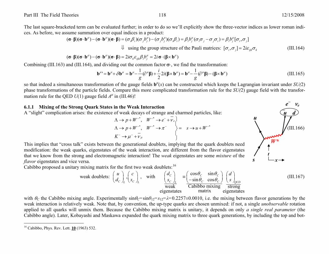
6.1.1 Mixing of the Strong Quark States in the Weak Interaction A “slight” complication arises: the existence of weak decays of strange and charmed particles, like:

* *

* * *

,,

ep W W ep W W s u W

K μ

ν

π

μ ν

− − −

− − − −

− −

⎫Λ → + → +⎪

Λ → + → = → +⎬⎪→ + ⎭

(III.166)

This implies that “cross talk” exists between the generational doublets, implying that the quark doublets need modification: the weak quarks, eigenstates of the weak interaction, are different from the flavor eigenstates that we know from the strong and electromagnetic interaction! The weak eigenstates are some mixture of the flavor eigenstates and vice versa. Cabibbo proposed a unitary mixing matrix for the first two weak doublets:16

cos sinweak doublets: , , with sin cosCabibbo mixingweak strong

matrixeigenstates eigenstates

C C C

C C C C C QCDL L L

du c dd s s s

θ θθ θ

⎛ ⎞ ⎛ ⎞⎛ ⎞ ⎛ ⎞ ⎛ ⎞≡ ⎜ ⎟⎜ ⎟ ⎜ ⎟ ⎜ ⎟ ⎜ ⎟− ⎝ ⎠⎝ ⎠ ⎝ ⎠ ⎝ ⎠ ⎝ ⎠ (III.167)

with θC the Cabibbo mixing angle. Experimentally sinθC=sinθ12=s12=λ=0.2257±0.0010, i.e. the mixing between flavor generations by the weak interaction is relatively weak. Note that, by convention, the up-type quarks are chosen unmixed: if not, a single unobservable rotation applied to all quarks will unmix them. Because the Cabibbo mixing matrix is unitary, it depends on only a single real parameter (the Cabibbo angle). Later, Kobayashi and Maskawa expanded the quark mixing matrix to three quark generations, by including the top and bot- 16 Cabibbo, Phys. Rev. Lett. 10 (1963) 532.

e− νe

⎯u d

W*

s

u

tx


tom quark states. The 3×3 unitary Cabibbo-Kobayashi-Maskawa (CKM) mixing matrix now has four real independent parameters: three mixing angles and a complex phase. The matrix may be constructed as a triple matrix product for rotational mixing between the generations 1 and 2, 1 and 3, and 2 and 3, with mixing angles θ12, θ13, and θ23, respectively, and with a single complex phase δ:

( ) ( ) ( )13 13 12 12

CKM 23 13 12 23 23 12 12

23 23 13 13

12 13 12 13 13

12 23 12 23 12 23 12 23 13

1, 1

1

iud us ub

cd cs cbi

td ts tb

i

i i

V V V c s e c sV V V R R R c s s cV V V s c s e c

c c s c s es c c s e c c s s s e s

δ

δ

δ

δ δ

θ θ δ θ

−

−

⎛ ⎞⋅ ⋅⋅ ⋅⎛ ⎞ ⎛ ⎞ ⎛ ⎞⎜ ⎟⎜ ⎟ ⎜ ⎟ ⎜ ⎟= = = ⋅ ⋅ ⋅ − ⋅⎜ ⎟⎜ ⎟ ⎜ ⎟ ⎜ ⎟⎜ ⎟ ⋅ ⋅⋅ − − ⋅ ⎝ ⎠⎝ ⎠ ⎝ ⎠⎝ ⎠

= − − −

V

( )

( )

2 3

2 223 13

3 212 23 12 23 13 12 23 12 23 13 23 13

1 21 2

1 1i i

A ic A

A i As s c c s e c s s c s e c cδ δ

λ λ λ ρ ηλ λ λ

λ ρ η λ

⎛ ⎞− −⎛ ⎞⎜ ⎟⎜ ⎟ ≈ − −⎜ ⎟⎜ ⎟

⎜ ⎟ ⎜ ⎟− − −− − −⎝ ⎠ ⎝ ⎠

(III.168)

Experientally, the diagonal CKM matrix elements are very close to unity, while the off-diagonal elements are small: λ = s12 ≡ sinθ12 = 0.2257±0.0010. The unitary CKM matrix may therefore be approximated up to O(λ3) by the last expression, the Wolfenstein parametriza-tion, in (III.168). The complex phase allows for CP-violation in the quark decays. CP-violation has been observed and measured in the neu-tral Kaon and B-meson systems. While very small in the Kaon system, it is rather large in the B-meson system. However, it turns out that this CP-violation is insufficient to explain, by itself, the observed dominance of matter over anti-matter in the universe. If there would be more than three generations of quarks, the CKM matrix would have to be expandedcorrespondingly. Therefore, the experimental measurement of the unitarity of the 3×3 matrix provides an important test for the SM with 3 generations. For example, unitarity requires:

( ) ( )

† * * *

3 3* *

* * 3 3

baseleft leg of right leg of

0

11 1 0

ud ub cd cb td tb

ud ub td tb

cd cb cd cb

V V V V V V

A i A iV V V VV V V V A A

λ ρ η λ ρ ηλ λ

Δ Δ

= ⇒ + + =

+ − −⇒ + + ≈ + + =

− −

VV 1

(III.169)

This describes a closed unitarity triangle in the complex plane. The closure, i.e. the exis-tence of only three generations, is being tested by a wide variety of experiments and found to be well satisfied within current experimental precision, see Figure 10. The la-bels at each contour indicate the measured quantity; e.g. the label “α” indicates the ex-periment measured the angle α of the unitarity triangle. Massive neutrinos can be incorporated into the Standard Model in the same way as mas-sive quarks, by coupling to the Higgs. Similar to the mixing in the “quark-sector”, lepton mixing can be incorporated in the lepton-sector if neutrinos have mass. This also implies the existence of heavy right-handed neutrino singlets; heavy in order to suppress their production. However, if present, such heavy right-handed neutrinos may have been pro-

Figure 10. 95%CL measurement contours of the unitarity triangle exhibiting the complex CP-violating phase (Fig. 11.2, PDG, Rev. of Part. Phys., Phys.Lett. B667 (2008) 1.)


duced in the very early universe, and may have survived to travel the universe without interacting (“relic neutrinos”). The right-handed leptons and quarks are all singlets under SU(2)L: they all have weak isospin zero.

6.2 The Radiation term in the SU(2) Lagrangian In close analogy to QED, see section, we will add to the Lagrangian a so-called radiation term of the form Lrad,SU(2) = –¼EμνEμν, with Eμν ≡ DμBν − DνBμ, where Dμ is the covariant derivative and Bμ ≡ ½σ⋅bμ. Bμ is a 2×2 matrix operator in SU(2) space, and bμ is the set of three fourvector (gauge) fields of the weak SU(2) vector bosons. Then:

( )1 1 1 1 12 2 2 2 2[ , ] 2

( ) ( ) ( )

[ , ]

( ) ( ) [ , ] ( )i j ijk ki

E D B D B igB B igB B B B ig B B B B

B B ig B B

ig g

μν μ ν ν μ μ μ ν ν ν μ μ ν ν μ μ ν ν μ

μ ν ν μ μ ν

μ ν ν μ μ ν μ ν ν μ μ νσ σ ε σ=

≡ − = ∂ + − ∂ + = ∂ − ∂ + − =

= ∂ − ∂ + =

= ∂ ⋅ − ∂ ⋅ + ⋅ ⋅ = ⋅ ∂ − ∂ −σ b σ b σ b σ b σ b b b ×b

(III.170)

clearly more complicated then the radiation term for QED! The extra complication arises from the fact that we are working with (Pauli) ma-trices here, which do not commute. The SU(2) symmetry is “non-Abelian”, whereas QED is Abelian.

6.3 The U(1)Y of Weak Hypercharge YW Clearly charge is not a good quantum number for the weak doublets, because the members have different charge. However, the quantity “Weak Hypercharge” YW ≡ 2(Q−IW

(3)) has unique values for the doublets:

1(3) 2

12

2 1(3) 3 2

1 13 2

2(0 )2( ) ( ) , 2( 1) ( ) , ( )

2( 1 ( ))

2( )2( ) ( ) , 2

2( ( ))

ee e eW R R R eR eR

L L LL

W RL L LL

Q I e e ee e ee

uu u uQ I ud d dd

νν ν νν ν− − −

− − −−

⎛ ⎞−⎛ ⎞ ⎛ ⎞ ⎛ ⎞= − = = − = − = − =⎜ ⎟⎜ ⎟ ⎜ ⎟ ⎜ ⎟− − −⎝ ⎠ ⎝ ⎠ ⎝ ⎠⎝ ⎠

⎛ ⎞−⎛ ⎞ ⎛ ⎞ ⎛ ⎞= − = = + =⎜ ⎟⎜ ⎟ ⎜ ⎟ ⎜ ⎟− − −⎝ ⎠ ⎝ ⎠ ⎝ ⎠⎝ ⎠

W W W

1W W3

Y 1 Y 2 Y 0

Y Y 23( ) ( ) , ( )R R R Ru u d d= + = −4 2

W3 3Y

(III.171)

i.e. the right-handed neutrino does not carry weak hypercharge, and as such does not participate in the weak interaction! We will impose the U(1)Y symmetry on the Lagrangian, similar to our earlier attempt to require symmetry under U(1) of charge which gave rise to electromag-netism.

6.4 The SU(3)C of Color It is now relatively straightforward to extend the discussion to higher-dimension gauge symmetries. The SU(3) of color symmetry is an ex-ample. The transformations under which we require the Lagrangian to be invariant are now taking place in three-valued color space. SU(3) phase transformations U(x) are generated by the group of 3×3 Hermitian lambda matrices λ = λi, i=1..8, of which there are exactly 8 inde-pendent ones: U(x) = exp{i½λ⋅g(x)}. The transformation properties under local gauge transformations are fixed by the group’s structure constants: [λi,λj]=fijkλk, where the fijk are the structure constants. The eight gauge boson fields Gμ

(i)(x), i=1..8, that need to be introduced in


the covariant derivative are the eight gluons of Quantum Chromo-Dynamics (QCD). Again, we cannot add mass terms for the gauge fields by hand; the gluons must be massless in order to preserve the local gauge invariance. Gauge fields are massless in Yang-Mills theories. Note that in non-Abelian Yang-Mills theories the radiation term in the Lagrangian contains terms – due to [Bμ,Bν] in (III.170) – that are powers of three and four in the gauge fields, hinting at the existence of 3-point and 4-point couplings between the gluons. In Abelian QED such terms are necessarily absent.

7 The Standard Model Lagrangian The Standard Model Lagrangian is constructed to be locally invariant under The U(1)Y of weak hypercharge, the SU(2)L of weak isospin, and SU(3)C of color. For our present discussion we will ignore the color group, because is not unified with the electromagnetic and weak interactions. In order to make the Lagrangian invariant under local gauge transformations U(x) of the particle fields, we are forced to introduce a “covari-ant derivative” Dμ of the proper form (the principle of minimal interaction):

( )

( )

(3) (1) (2)

(1) (2) (3)

'' 2 2 2( ) ( ) '2 2

2 2 2

ig ig iga b b ibig igD a x x ig ig igb ib a b

μ μ μ μ μ

μ μ μ μ μ

μ μ μ μ μ

⎛ ⎞∂ + + −⎜ ⎟∂ → = ∂ + + ⋅ = ⎜ ⎟

⎜ ⎟+ ∂ + −⎝ ⎠

W

W

W

YY σ b

Y (III.172)

This is the electroweak part of the covariant derivative in the Standard Model, with the aμ(x) gauge vector field (indicated by the Lorentz index μ) of the weak hypercharge symmetry, and the triplet of gauge vector fields bμ(x) of the weak isospin symmetry. The full electroweak Lagrangian contains the following terms: 1. Free-particle (kinetic) terms for all weak fermionic doublets and singlets; interactions are specified by the replacement of derivatives by

the covariant derivative. In this way, the gauge fields are introduced with a very specific form and couplings. The leptons and quarks must obey the Dirac equation, and we expect the particle terms to mimic the Dirac Lagrangian:

, , with ( ) , , Dirac spinorse

eeLe L L L e

L

L i D x eee

μν μ

ννψ γ ψ ψ ψ ν −

−−⎛ ⎞⎛ ⎞= = = =⎜ ⎟ ⎜ ⎟

⎝ ⎠ ⎝ ⎠L

L

PP

(III.173)

2. A free-particle, Klein-Gordon type, term for the Higgs field, together with the Higgs potential with the famous non-zero vacuum expec-tation value. The Higgs field is a SU(2) doublet of complex scalar fields, i.e. four independent real scalar fields. The Higgs field, with a non-zero vacuum expectation value, will give mass to three vector boson fields.

3. Free-field terms for the bosonic gauge fields. For the SU(2) part we take, in close analogy to the U(1) QED Lagrangian, the form Lrad,SU(2) = –¼EμνEμν, with Eμν ≡ DμBν − DνBμ, where Bμ ≡ ½σ⋅bμ. Bμ is a 2×2 matrix operator in SU(2) space. The Dμ will give rise to self-interactions between the gauge bosons.

7.1 A Higgs Field in SU(2) As for QED, we may postulate a Lagrangian L for a scalar (Higgs) field φ that is a SU(2) weak isospinor:


( ) ( ) ( )2† 2 42 2 2 † 2 †1 2

3 4

1, with , and potential 2

iL V Viμ

μϕ φφ φ φ μ φ λ φ μ φ φ λ φ φϕ φ

+⎛ ⎞= ∂ ∂ − = = + = +⎜ ⎟+⎝ ⎠ (III.174)

For positive μ2 this decribes an iso-doublet of two complex fields, or four real fields φI, all of mass μ. Note that, as for all weak isospin dou-blets, the upper member of the doublet must have one unit of charge more than the lower member. The Lagrangian exhibits global gauge invariance for SU(2) transformations:

1' exp2

iφ φ φ⎛ ⎞→ = ⋅⎜ ⎟⎝ ⎠

σ β (III.175)

If we demand local gauge invariance for SU(2) transformations, we must introduce a set of three gauge fields bμ(x) to form covariant deriva-tive Dμ:

2gD iμ μ μ= ∂ + ⋅σ b , with transformation properties 1' ( ) ( )g

μ μ μ μ= − ∂ − ×b b β β b .

As before, we next consider a Higgs-type potential with μ2<0. As before, we may choose the simplest vacuum, a real local minimum with φ1=φ2=φ4=0, φ3=v=|μ|/λ, and re-write the Lagrangian for departures φ’ from this minimum. This will generate a mass term for the field φ’ (as well as for the three gauge bosons):

( ) ( ) ( )

( ) ( )

22 2 42 † 2 † 2

2

2 22 2 2 4 3 2 2 3 4 2 2 2 2 2 3 4

2 2

1 1( ') ' ' ' ' ( ) ( )2 4

1 1 12 4 6 42 4 4 4

V v x v xv

v v v v v v v vv v

μφ μ φ φ λ φ φ μ η η

μ μμ η η η η η η μ μ η μ η η

= − + = − + + +

= − + + + + + + + = − + + +

(III.176)

We will see below that this will lead to the desired result: a theory with local gauge invariance which is “hidden” and with gauge vector fields that now have mass terms. Note, that this lower member of the doublet, the physical vacuum, must be neutral because it must be in-variant under the UQ(1) group of transformations of electromagnetism, U=exp[iα(x)Q], to prevent the photon from acquiring a mass!

7.2 The Vector Boson Masses As we argued before, it is imperative for a realistic theory that the weak gauge bosons be massive. The Higgs mechanism will accomplish that. The term that is of importance is the Klein-Gordon term for the scalar Higgs field doublet φ (which has weak hypercharge +1):

( )( )

(3) (1) (2)

(1) (2) (3) 0

(3) ( )

( ) (3) 0

'' 2 2 2( ) ( ) '2 2

2 2 2'

2 2 2'

2 2 2

ig ig iga b b ibig igD a x x ig ig igb ib a b

ig ig iga b b

ig ig igb a b

μ μ μ μ μ

μ μ μ μ

μ μ μ μ μ

μ μ μ μ

μ μ μ μ

φφ φ

φ

φ

φ

+

+−

+

⎛ ⎞⎛ ⎞∂ + + −⎜ ⎟⎛ ⎞ ⎜ ⎟= ∂ + + ⋅ = =⎜ ⎟⎜ ⎟ ⎜ ⎟⎝ ⎠ ⎜ ⎟+ ∂ + − ⎝ ⎠⎝ ⎠⎛ ⎞⎛∂ + +⎜ ⎟⎜= ⎜ ⎟⎜ ⎟∂ + − ⎝⎝ ⎠

W

W

W

YY σ b

Y

, ( 1 )φ φ⎞⎟ = +

⎜ ⎟⎠

WY

(III.177)


Note, as argued before, the physical Higgs field must be neutral. Moreover, the Higgs iso-doublet members must have weak isospin ±½, and the top member must be larger in charge than the bottom member by one unit of e. Therefore, we can choose the Higgs doublet either as φ=(φ+,φ0) (YW=+1) or as φ=(φ0,φ–) (YW=–1). As we’ve shown in section 7.1 above, the Higgs field may be re-written around the true vac-uum, which without loss of generality may be chosen as φ+= (0,0), φ0= (0,v/√2), with ν=|μ|/λ = real. After using the gauge invariance of the Lagrangian to “rotate away” the three (!) scalar fields ζ(x), the Higgs field turns into [v+η(x)]/√2. To check, we can rotate “back” the with the rotation exp(+iσ·ζ/2v):

( )3 1 22 12

to first order1 2 3 3in small fields( ) and ( )

2 2

2 2

11 1 1 1 20 0 01( ) ( ) ( ) ( ) 222 2 2 21i

iv

x x

iv v

iv v

i i ie iv x v x v x v x iv i iη ζ

ζ ζ ζ

ζ ζ ζζ ζφ η η η η ζ

⋅−

+

⎛ ⎞+ +⎛ ⎞⎛ ⎞⎛ ⎞ ⎛ ⎞ ⎛ ⎞⎜ ⎟= + ⋅ =⎜ ⎟ ⎜ ⎟ ⎜ ⎟⎜ ⎟ ⎜ ⎟+ + + + −⎜ ⎟⎝ ⎠ ⎝ ⎠ ⎝ ⎠⎝ ⎠ − ⎝ ⎠⎝ ⎠

σ ζ σ ζ ,

to find again the set of four real fields, or two complex fields, we started out with… The covariant derivative of the neutral Higgs field becomes:

( )

1 1 1(3) ( )2 2 2

0 01 1 1( ) (3)2 2 2

1 ( ) 02 0 0

1 1 (3) 02 2

'0 01 1( ) '2 2

( )1 , ( )' ( )2

ig a igb igbD D

v x vigb ig a igb

igb vig a igb v

μ μ μ μμ μ

μ μ μ μ

μ

μ μ μ

φη η

ηη η

η

−

+

−

⎛ ⎞∂ + +⎛ ⎞ ⎛ ⎞= = =⎜ ⎟⎜ ⎟ ⎜ ⎟⎜ ⎟+ +∂ + −⎝ ⎠ ⎝ ⎠⎝ ⎠⎛ ⎞+

= = +⎜ ⎟⎜ ⎟∂ + − +⎝ ⎠

W

W

W

YY

Y

(III.178)

Taking μ=|μ|>0, i.e. as positive and real, and using the Higgs potential V(φ)= –μ2|φ|2+λ2|φ|4 from equation (III.176) above, rewritten around the vacuum expectation value v=μ/λ, the Lagrangian part for the Higgs field becomes:

2† ( ) ( ) 2 (3) 2 2

2 2 ( ) ( ) 2 (3) 2

Higgs Kinetic mass term mass term

2 2 2 3 4

Higgs mass

1 1( ) ( ) ( ) ( )( ) ( ) ( ' ) ( ) ( )2 8 8

1 1 1( )( ) ( ' )2 8 8

( 4/ /

Higgs

W Z

gL D D V b b v g a gb v V v

g v b b v g a gb

v v

μ μ μμ μ μ μ μ

μ μμ μ μ μ

φ φ φ η η η η η

η η

μ η μ η η

+ −

+ −

= − = ∂ ∂ + + + − + − + =

= ∂ ∂ + + −

− − + 2 2 2

Higgs self couplings constant term

2 ( ) ( ) 2 ( ) ( ) 2 (3) 2 (3) 2 2

Couplings between s, s, and Higgses; NOT to photon!

) 4

1 1 1 1( ' ) ( ' )4 8 4 8

W Z

v

g vb b g b b v g a gb g a gbμ μμ μ μ μ μ μ

μ

η η η η+ − + −

+

+ + + − + −

(III.179)

where we find mass terms for three of the four gauge bosons of UY(1)×SUL(2). These mass terms imply three more degrees of freedom for the gauge fields which – being massless – originally only had transverse polarizations, but now acquire a longitudinal polarization in addi-tion! These degrees of freedom come from the three fields ζi which have disappeared from the Lagrangian and were “absorbed” into the gauge fields. One gauge field remains massless. From the above it is clear that we can construct massive W± and Z0 bosons as linear combi-


nations of the aμ and bμ fields, while the Higgs does not couple to the photon (defined as the state orthogonal to the Z) which therefore re-mains massless:

( )

(3)0

2 2 2 2

(3)(3)

2 22 2

12

' '

' '''

''

W b

g a gb gA g ZZ a

g g g gg A gZga g b bA

g gg g

μ μ

μ μ μ μμ μ

μ μμ μμμ

± ≡

⎫− + −⎧≡ =⎪ ⎪

+ +⎪ ⎪⇔⎬ ⎨ ++ ⎪ ⎪ =≡ ⎪ ⎪ ++ ⎩⎭

∓

(III.180)

Then we can identify (note the factor ½ for a correct neutral vector boson mass term like the photon):

( ) ( )0

0

2 22 2 2 21 1 1 1 12 2 ( ) ( ) 2 2 ( ) ( ) 2 28 8 2 2 8

21 12 (3) 2 2 2 2 0 2 2 2 28 8

2

4 21( ' ) ( ' ) ' 1 '2

with arctan( ' ) 1 tan cos

W

WZ

W W W W WZ

g v gvg v b b g v b b g v W W M

v g a gb g g v Z M v g g M g g

g g M M M

μμ μ μ μ μ

μ μ μ

θ θ θ

±+ − + − − += + = + ⇒ = =

− = + ⇒ = + = +

≡ ⇒ = + =

(III.181)

where we have defined the Weinberg angle θW, which defines the physical particles, the Z0 and the photon, in terms of mixtures of the neu-tral fields bμ

(3) and aμ. In case there were no mixing between the U(1)Y and SU(2)L neutral gauge bosons, we would have g’=0. Then θW=0 and the W± and Z0 bosons would have had the same mass. Note, that g’=0 implies e=0, see the next section!

7.3 The Interactions between the Gauge Bosons and the Fermions The interactions of the elementary fermions, leptons and quarks, arise naturally from Dirac terms in the Lagrangian: Lint=⎯ℓ iγμDμ ℓ, with ℓ a lefthanded weak isospin doublet of leptons or singlet, and Dμ the covariant derivative. We will use the interaction terms to fix the coupling to the physical photon to the experimental value e, where α ≡ e2/4π = 1/137. Taking the electron-neutrino doublet as example we find:


( ) ( ) ( )

( ) ( ) ( )( )2 2

2 2

1 1 12 2 2

12 22 2 21 2 2 '2 2 '

' ( ) ( ) ' ( )

'( ' '

( ' ) 2 '

kinetic terms f

eint e R RL

L

iie

e R RiL g gLg g

L e i ig a x ig x e i ig a x ee

g g Z igWe i e i g Z gg A eeigW g g Z gg A

μ μμ μ μ μ μ

μ μ μμ μμ μ μ

μ μ μ μ

νν γ γ

νν γ γ+

− ++

⎛ ⎞= ∂ + + ⋅ + ∂ + =⎜ ⎟⎝ ⎠

⎛ ⎞∂ + + ⎛ ⎞⎜ ⎟= + ∂ + −⎜ ⎟∂ + − −⎜ ⎟⎝ ⎠⎝ ⎠

=

W WY σ b Y

( )

( )

2 2

2 22

2 2 2 2

'or and

2 2' 1 ' '

2' '

e L L L L L L

L L R R L L R R

g g ge v Z e W e W

gg g ge e e e A e e g e e Zg g g g

e e

μ μ μμ μ μ

μ μ μ μμ μ

μ

ν γ ν ν γ γ ν

γ γ γ γ

γ

+ −++ + − +

⎛ ⎞−+ + + −⎜ ⎟

+ + ⎝ ⎠=

(III.182)

Fixing the photon coupling, we need e = gg’/√(g2+g’2) = gsinθW. The W coupling is fixed by the highly accurate measurement of the muon lifetime, which gives the Fermi constant GF (measured with muons in a circular storage ring where they have a well known momentum):

2 2

2 2 2

1 1 12 8 22 2

F

W W

G g gM M v

⎛ ⎞= = =⎜ ⎟⎝ ⎠

(III.183)

see equation (III.181). This implies, for instance, that v= 246 GeV. It can be seen that the Standard Model predicts the existence of weak “neutral currents” mediated by the Z0, in addition to the weak “charged currents” mediated by the charged gauge bosons W±. Neutral cur-rents are not easily seen in decays (e.g. μ− → μ− + Z0*, Z0*→⎯ν + ν violates energy-momentum conservation), and appear clearly only in interactions. At low energy, only neutrino interactions are feasible for a study of weak neutral currents, because electromagnetic neutral-current events, mediated by the photon, drown out the weak interaction by many orders of magnitude! Eventually, in 1973, a handful of neu-tral current events was seen at CERN. The coupling between the electron and the Z boson can be written in terms of the vector and axial-vector couplings cV and cA:

2 2 2 22 2 2

2 2 2 2

2 2 2 22 2

2 2 2 2

2 5

1 ' 1 '' ' '2 2' '

1 ' 1 '' '2 2' '

1 12sin2cos 2 2 2cos

L L R R L L

L L

W VW W

g g g ge e g e e Z g e e g e e Zg g g g

g g g ge P g eZ e P g eZg g g g

g ge eZ e c

μ μ μ μμ μ

μ μμ μ

μμ

γ γ γ γ

γ γ

θ γ γθ θ

⎛ ⎞⎛ ⎞ ⎡ ⎤− −− = + −⎜ ⎟⎜ ⎟ ⎢ ⎥

+ +⎝ ⎠ ⎣ ⎦⎝ ⎠

⎛ ⎞ ⎛ ⎞+ += − = −⎜ ⎟ ⎜ ⎟

+ +⎝ ⎠ ⎝ ⎠

⎛ ⎞= − − + + = −⎜ ⎟⎝ ⎠

( )5Ac eZμ

μγ γ

(III.184)

For the quarks, the coupling to the Z is similar: the vector and axial-vector couplings of the Z to fermions in terms of the U(1)Y and SU(2)L groups are as the last expression in (III.184), with cV=I3 – 2Qsin2θW, cA= I3.


In summary, in the Standard Model, we find a number of “arbitrary” parameters: g, g’, μ2, and v. Three of these: g, g’, and v; can be related to extremely well-measured experimental quantities: e, MZ=91,187.6±2.1 MeV, GF.=1.16637×10–5 GeV2. Other parameters: sin2θW, MW can then be predicted/calculated and compared to experiment as a check on the Standard Model. The parameter μ2 is only related to the Higgs boson mass; until the Higgs is found, it remains essentially unknown. However, consideration of higher order terms in Feynman diagrams tells us, that if the ‘t Hooft-Veltman cancellations are to work in higher order diagrams (renormalizability of the Standard Model), the Higgs mass cannot be very much higher than the weak gauge boson masses: mH <1000 GeV.

7.4 Fermion Masses Because the basic fields in the Standard Model are the SU(2) doublets and the singlets, simple Dirac mass terms of the form m⎯ℓℓ are not gauge invariant: the neutrino and the electron have different masses. Under SU(2) weak isospin rotations, the Dirac spinor e = (PLe + PRe) = (eL + eR) will change: the eL being part of a doublet mixes with the neutrino under SU(2) rotations, whereas eR , a SU(2) singlet, does not. Again, the Higgs mechanism helps out: we introduce SU(2)-invariant interaction terms of the type (taking mν=0):

( ) ( )

( )

†0

2 2

1 0, with , ,( )2

( ) ( )2 2 2

Higgs to coup mass: ; 2

elepton Higgs R L L R L R R

L

e e eR L L R R L L R R L L R

e e ee e F

L g ev x eg g gv x e e e e v e e e e x e e e e

eg g me m v m Gv

νφφ φ φ ηφ

η η

+

−−⎛ ⎞ ⎛ ⎞⎛ ⎞⎡ ⎤= − + = → = =⎜ ⎟⎜ ⎟ ⎜ ⎟⎣ ⎦ +⎝ ⎠ ⎝ ⎠⎝ ⎠

⎡ ⎤ ⎡ ⎤ ⎡ ⎤= − + + = − + − +⎣ ⎦ ⎣ ⎦ ⎣ ⎦

= = = ling

(III.185)

Because φ†ℓL and⎯ℓLφ are SU(2) scalars, being dot-products of SU(2) weak isospinors, both terms in Llepton-Higgs are scalars under SU(2)L transformations. Also, the neutrino is left massless and does not couple to the Higgs! The couplings of the charged leptons to the Higgs are “fixed” experimentally by the measured fermion mass: e.g. ge=me/v= 2.1×10–6. In this way, for each massive fermion we introduce an a-priori arbitrary coupling constant gℓ, a total of nine (or twelve, because neutrinos have mass) additional parameters! Rather unsatisfactory... Quark masses are read off the Lagrangian as well. For the down-type quarks:

( ) ( )

( )

†0

2 2

1 0, with ,( )2

( ) ( )2 Higgs to coupling mass: ; 2

d Higgs d R L L R LL

dR L L R d R L L R d R L L R

d dd d F

uL g d q q d qv x d

g v x d d d d g v d d d d g x d d d ddg gd m v m G

φφ φ φ ηφ

η η

+

−⎛ ⎞ ⎛ ⎞ ⎛ ⎞⎡ ⎤= − + = → =⎜ ⎟ ⎜ ⎟⎜ ⎟⎣ ⎦ +⎝ ⎠ ⎝ ⎠⎝ ⎠

⎡ ⎤ ⎡ ⎤ ⎡ ⎤= − + + = − + − +⎣ ⎦ ⎣ ⎦ ⎣ ⎦

= =

(III.186)

However, this leaves the up-type quarks massless (like the neutrino)! Again, SU(2) symmetry helps us out: we construct a charge-conjugate Higgs doublet φc in a way completely analogous to the construction of the SU(2) strong isospin anti-doublet, see (I.47):


0

*2

( )102c

v xi

ηφφ σ φφ −

+⎛ ⎞ ⎛ ⎞−= − = →⎜ ⎟ ⎜ ⎟⎝ ⎠⎝ ⎠

(III.187)

Using φc, which has an upper component after the SU(2)L symmetry breaking, we may give mass to the up-type quarks:

( ) ( )

( )

0†

2 2

1 ( ), with ,02

( ) ( )2 Higgs to coupling mass: ; 2

u Higgs u R c L L c R c LL

uR L L R u R L L R u R L L R

u uu u F

v x uL g u q q u q d

g v x u u u u g v u u u u g x u u u uug gu m v m G

ηφφ φ φφ

η η

− −

⎛ ⎞ +⎛ ⎞ ⎛ ⎞−⎡ ⎤= − + = → =⎜ ⎟ ⎜ ⎟ ⎜ ⎟⎣ ⎦ ⎝ ⎠ ⎝ ⎠⎝ ⎠

⎡ ⎤ ⎡ ⎤ ⎡ ⎤= − + + = − + − +⎣ ⎦ ⎣ ⎦ ⎣ ⎦

= =

(III.188)

Clearly, this is a way to also account for neutrino masses if so needed… Note, that the Higgs couples to a fermion in proportion to its mass, i.e. a 100 GeV Higgs decays mostly to a pair of b-quarks.

Documents

5.1 A One-dimensional Higgs Modelsbhepnt.physics.sunysb.edu/~rijssenbeek/PHY557_F08_L10.pdf5 The Higgs Mechanism ... of a boson field with an odd shape, i.e. a non-zero expectation