94

5.1 Stream gauging site selection

The principles of network design and the proposed use of data should govern the

selection of streams to be gauged. Dense network of gauging station is required

for research works related to runoff estimation, soil erosion estimation, and water

balance calculation at different watershed sizes. Whereas the goal is to construct a

dam to impound water, light network of stream gauging stations is sufficient -

one station at or near the dam site can be adequate. A general-purpose network

must, however, provide the ability to estimate hydrological parameters over a

wide area using for example a regional regression model.

Despite the development of a variety of objectives and statistically based methods

for streamflow and rainfall network design, judgment and experience are still

Continuous streamflow records are necessary in the design of water supply

systems, in designing hydraulic structures, in the operation of water management

systems, and in estimating sediment or chemical loads of streams. To do these,

systematic records of stage and discharge are essential. This chapter elaborates

common methods practiced in Ethiopia to measure streamflow.

River stage is the elevation above some arbitrary zero datum of the water surface

at a streamflow gauging station. The datum is sometimes taken as mean sea level

but more often is slightly below the point of zero flow at the gauging station. The

elevation datum is set with reference to at least three permanent reference marks

or benchmarks located in stable ground separate from the recorder structure

following standard surveying work.

It is difficult to make a direct, continuous measurement of discharge in a stream

or river but relatively simple to obtain a continuous record of stage. Thus

measurements of river stage provides the best alternative. Before we discuss some

methods of measuring river stage, first we discuss criteria fort selecting a stream

gauging station.

5. STREAMFLOW MEASUREMENTS

95

indispensable. The WMO Guide to Hydrological Practice recommendations for

network density as a staring point for network design is given in Table 5.1.

Table 5-1.Recommended minimum density of hydrometric stations

Type of region

Range of norms for

minimum network, area,

km2 per station

Range of provisional

norms tolerated in

difficult conditions area,

km2 per station

Flat regions of tropical,

temperate and

Mediterranean zones

1000 - 25000

3000 - 10000

Mountainous regions of

tropical, temperate and

Mediterranean zones

300 -100

1000 - 5000

Small mountainous

islands with very

irregular rainfall, very

dense stream network

140 - 300

Arid zone 5000 - 20000

5.1.1 Selection of gauging site

The selection of a particular site for the gauging station on a given stream should

be guided by the following criteria for an ideal gauge site (WMO 1981):

i. The general course of the stream is straight for about 100 meters upstream

and downstream from the gauging site.

ii. The total flow is confined into the channel at all stages and no flow

bypasses the site as sub-surface flow.

iii. The streambed is not subject to scour and fill and is free of aquatic growth.

iv. Banks are permanent, high enough to contain floods, and are free of brush.

v. Unchanging natural controls are present in the form of a bedrock outcrop

or other stable riffle for low flow, and a channel constriction for high flow,

or a fall or cascade that is un-submerged at all stages to provide a stable

96

relation between stage and discharge. If no satisfactory natural low-water

control exists, a suitable site is available for installing an artificial control.

vi. A site is available, just upstream from the control, for housing the stage

recorder where the potential for damage by water-borne debris is minimal

during flood stages; the elevation of the stage recorder itself should be

above any floods likely to occur during the life of the station.

vii. The gauge site is far enough upstream from the confluence with another

stream.

viii. A satisfactory reach for measuring discharge at all stage is available

within reasonable proximity of the gauge site. It is not necessary that low

and high flows be measured at the same cross-section.

ix. The site is readily accessible for ease in installation and operation of the

gauging station.

x. Facilities for telemetry can be made available, if required.

xi. Typical streamflow gauging station installed in the Wabi Shebele river at

upstream fo Melka Wakana Dam is shown in Figure 5.1. In practice rarely

will an ideal site be found for a gauging station and judgement must be

exercised in choosing between possible sites. A gauging site should be

located at a point along the stream where there is a high correlation

between stage and discharge, featuring a one to one correspondence

between stage and discharge. Either section or channel control is

necessary for the rating to be single-valued.

xii. A rapid or fall located immediately downstream of gauging site forces

critical flow through it, providing a section control. In the absence of a

natural section control, an artificial control – for instance, a concrete weir

– can be built to force the rating being single-valued. This type of control

is very stable under low and average flow conditions.

xiii. A long downstream channel of relatively uniform cross-sectional shape,

constant slope, and bottom friction provides a channel control. However, a

97

gauging site relying on channel control requires periodic re-calibration to

check its stability. To improve channel control, the gauging site should be

located far from downstream backwater effects caused by reservoirs and

large river confluence.

Figure 5-1: Typical streamflow gauging station installed in the Wabi river

near Dodola town upstream of the Melkawakana reservoir (February 2002).

5.2 Stage measurement

Basically there are two modes of stage measurements. The first is discrete stage

measurements using manual gauges, and the second is continuous stage

measurements using recorders. For the measurement of stage, uncertainties

should not be worse than 10 mm or 0.1 % of the range.

5.2.1 Manual gauge

The simplest way to measure river stage is by means of a staff gage. A staff gauge

is vertically attached to a fixed feature such as a bridge pier or a pile (Figure 5.2).

The scale is positioned so that all possible water levels can be read promptly and

accurately. Another type of manual gauge is the wire gauge. Wire gauge consists

of a reel holding a length of light cable with a weight affixed to the end of the

Watershed properties

_______________________________________________________________________________ 98

cable. The reel is mounted in affixed position – for instance, on a bridge span –

and the water level is measured by unreeling the cable until the weight touches the

water surface. Each revolution of the reel unwinds a specific length of cable,

permitting the calculation of the distance to the water surface. Manual gages are

used where stages do not vary greatly form one measurement to another

measurement. They are impractical in small or flashy streams, where substantial

changes in stages may occur between readings.

5.2.1 Recording gauge

A recording gage measures stages continuously and records them on a strip chart.

The mechanism of a recording gauge is either float actuated or pressure actuated.

In a float actuated recorder, a pen recording the water level on a strip chart is

actuated by a float on the surface of the water. The recorder and float is housed on

suitable enclosure on the top of a stilling well connected to the stream by two

intake pipes (two intake pipes are used incase one of them become clogged)

(Figure 5.2). The stilling well protects the float from debris and ice and dampens

the effect of wave action. This type of gage is commonly used for continuous

measurements of water levels in rivers and lakes.

The pressured actuated recorder or the bubble gage senses the water level by

bubbling a continuous stream of gas (usually CO2) into the water. The bubble

gauge consists of a specially designed servo-manometer, gas-purge system, and

recorder. Nitrogen fed through a tube bubble freely into the stream through an

orifice positioned at a fixed location below the water surface. The pressure in the

tube, equal to that of the piezo-meteric head above the orifice, is transmitted to the

servo-manometer, which converts changes in pressure in the gas-purge system

into pen movements on a strip-chart recorder. Bubble-type water level sensors are

used in applications where a stilling well is either impractical or too expensive

and where the stream carries a heavy sediment load. The Awash river at Awash

town is equipped with pressured actuated recorder.

99

Figure 5-2. The measurement of stage through manual methods and recording

instruments (after Gregory and Walling, 1973)

100

Figure 5-3: A typical chart from vertical float recorder.

101

Crest stage gage. This is used to obtain a record of flood crest at sites where

recording gages are not installed. A crest stage gage consists of a wooden staff

gage scale, situated inside a pipe that has small holes for the entry of water. A

small amount of cork is placed in the pipe, floats as the water rises, and adheres to

the staff or scale at the highest water level.

Telemetric gages. Gages with automatic data transmittal capabilities are called

self-reporting gages, or stage sensors. Self-reporting gauges are of the float-

actuated or pressure actuated type. These instruments use telemeters to broadcast

stage measurement in real time, from a stream gauging location to a central site.

This type of gauge is ideally suited for applications where speed of processing is

of utmost important, e.g., for operational hydrology or real-time flood forecasting.

102

5.3 Flow velocity measurement and discharge computation

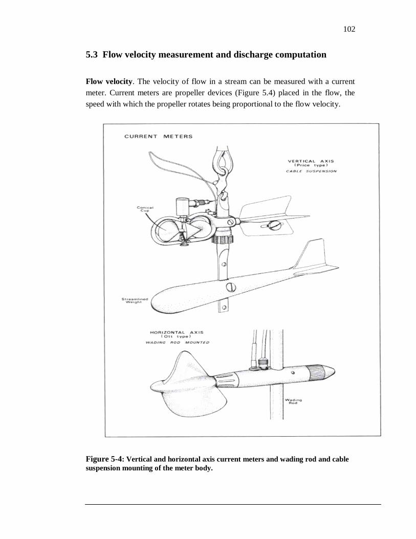
Flow velocity. The velocity of flow in a stream can be measured with a current

meter. Current meters are propeller devices (Figure 5.4) placed in the flow, the

speed with which the propeller rotates being proportional to the flow velocity.

Figure 5-4: Vertical and horizontal axis current meters and wading rod and cable

suspension mounting of the meter body.

Watershed properties

_______________________________________________________________________________ 103

The relation between measured revolution per second of the meter cups N and

water

velocity V is given by

where:

a = the starting velocity or velocity required to overcome mechanical friction.

b = the constant of proportionality, and

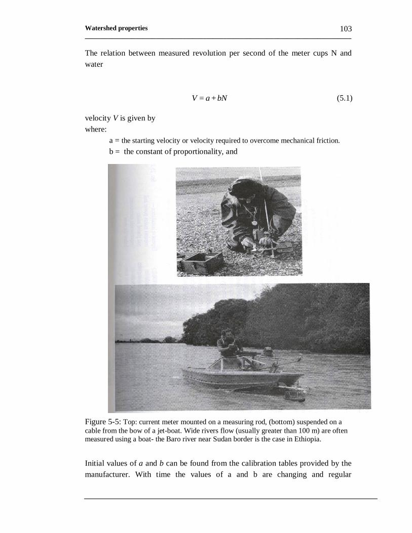
Figure 5-5: Top: current meter mounted on a measuring rod, (bottom) suspended on a

cable from the bow of a jet-boat. Wide rivers flow (usually greater than 100 m) are often measured using a boat- the Baro river near Sudan border is the case in Ethiopia.

Initial values of a and b can be found from the calibration tables provided by the

manufacturer. With time the values of a and b are changing and regular

bN + a = V (5.1)

104

recalibration is essential. This may be done by towing the current meter through

still water in a tank at a series of known velocities.

The current meter can be hand-held in the flow in a small stream (measurement

by wading), suspended from a bridge or cable way across a large stream, or

lowered from the bow of a boat (Figure 5.5).

Velocity distribution: The flow velocity varies with depth in a stream . Over the

cross-section of an open channel, the velocity distribution depends on the

character of the river banks and of the bed and on the shape of the channel. The

maximum velocities tend to be found just below the water surface and away from

the retarding friction of the banks.

The average velocity occurs say about 0.6 of the depth. It is standard practice to

measure velocity at 0.2 and 0.8 of the depth when the depth is more than 60 cm

and to average the two velocities to determine the average velocity for the vertical

section. For shallow rivers and near the banks on deeper rivers where the depths

are less than 0.6 m, velocity measurements are made at 0.6 of depth of flow.

Discharge computation.

The discharge computation of a stream is calculated from measurements of

velocity and depth. A marked line is stretched across the stream. At regular

intervals along the line, the depth of the water is measured with a graduated rod or

by lowering a weighted line from the surface to the stream bed, and the velocity is

measured using a current meter. The discharge Q at a cross-section of area A is

found by

(5.2)

Where V = streamflow velocity

A = cross sectional area of the flow

dAVQ .

105

Figure 5-6. The velocity area technique of discharge measurements: a cable way is used

on large streams for positioning the current meter in the verticals and a special cable

drum can be used to obtain accurate readings of depth and spacing of verticals. The mean

section and mid-section methods are commonly used to compute the discharge of the individual segments.

106

in which the integral is approximated by summing the incremental discharges

calculated from

each measurement i, i = 1, 2, ..., n of velocity Vi and depth di.

The measurements represent average values over width wi of the stream.

Example 5.1: Given the following stream gauging data, calculate the discharge.

Vertical No. 1 2 3 4 5 6 7 8 9 10 11

Distance to refernce point (m) 15.0 20.0 25.0 30.0 35.0 40.0 45.0 50.0 55.0 60.0 65.0

Sounding depth di (m) 0.0 0.5 0.8 1.2 1.5 2.5 3.0 2.0 1.2 2.7 2.9

Velocity at 0.2 di (m/s) 0.0 0.5 0.7 0.9 1.2 1.4 1.7 1.3 0.9 1.7 1.8

Velocity at 0.8 di (m/s) 0.0 0.4 0.6 0.7 0.8 1.1 1.3 1.0 0.7 1.3 1.4

Solution: To use Eq. (5.3) first the average velocity at each sounding depth is calculated,

then the partial width which is constant in this example is calculated (20-15) = 5 m

Vertical No. 1.0 2.0 3.0 4.0 5.0 6.0 7.0 8.0 9.0 10.0 11.0

Distance to reference point (m) 15.0 20.0 25.0 30.0 35.0 40.0 45.0 50.0 55.0 60.0 65.0

Sounding depth (m) 0.0 0.5 0.8 1.2 1.5 2.5 3.0 2.0 1.2 2.7 2.9

Velocity at 0.2 m (m/s) 0.0 0.5 0.7 0.9 1.2 1.4 1.7 1.3 0.9 1.7 1.8

Velocity at 0.8 m (m/s) 0.0 0.4 0.6 0.7 0.8 1.1 1.3 1.0 0.7 1.3 1.4

Average Velocity (m/s) 0.0 0.5 0.7 0.8 1.0 1.3 1.5 1.2 0.8 1.5 1.6

Partial area Ai (msq) 0.0 2.5 4.0 6.0 7.5 12.5 15.0 10.0 6.0 13.3 4.8

Partial discharge (m3/s) 0.0 1.1 2.6 4.8 7.5 15.6 22.5 11.5 4.8 19.5 7.6

Total Q = 97.58 (m3/s) Total A = 81.61 msq

Average velocity (m/s) = Q/ A = 1.196 m/s

-3.5

-3.0

-2.5

-2.0

-1.5

-1.0

-0.5

0.0

1 2 3 4 5 6 7 8 9 10 11

WdV = Q iii

n

=1i

(5.3)

107

5.4 Dilution gauging

Dilution gauging method of measuring the discharge in a stream is made by

adding a chemical solution or tracer of known concentration to the flow and then

measuring the dilution of the solution downstream where the chemical is

completely mixed with the stream water. A tracer is a substance that is not

normally present in the stream and that is not likely to be lost by chemical

reaction with other substances. Salt, fluorescein dye, and radioactive materials are

commonly used as tracers. In general there are two methods of dilution gauging,

sudden-injection methods and constant rate injection method. The two methods

are described as follows.

5.4.1 Sudden Injection method

In this method a quantity of tracer volume V1 and concentration C1 is added to the

river by suddenly emptying a flask of tracer solution that is gulp injection. At the

sampling station downstream the entire tracer cloud is monitored to find the

relation between concentration and time. The quantity of tracer or mass of tracer

M is then equal to C1V1. If t1 is the time before the leading edge of the tracer

cloud arrives at the sampling station and t2 is the time after all the tracer has

passed this station the quantity of tracer is given by

Where: C2 = sustained final (equilibrium) concentration of the chemical in the

well mixed flow (mg/l)

C0 = the base value concentration, already present in the river (mg/l)

Using principle of conservation of mass we may estimate the streamflow Q:

C1V1 = dtCCQ

t

t

)( 02

2

1

(5.5)

dtCC

VCQ

t

t

)( 02

11

2

1

(5.6a)

108

2

11

TC

CVQ (5.6b)

Figure 5-7. Dilution gauging: constant rate injection and gulp injection.

109

5.4.2 Continuous and constant rate injection method

In this method a tracer of known concentration C1 is injected continuously at a

rate q at a sampling station situated downstream of injection point. The mass rate

M at which the tracer enters the test reach is

Assuming that satisfactory mixing of tracer has taken place with the entire flow

across the cross-section with the measured concentration C2 (reaching equilibrium

concentration), we have

201 )( CqQQC qC (5.8)

Solving for Q we get

qC C

C CQ

02

21

(5.9a)

The dilution method is particularly useful for very turbulent flows, which can

provide complete mixing within a relatively short distance. It is also applicable

when the cross section is so rough that alternative methods are unfeasible.

It is to be noted that a highly turbulent and narrow reach is desirable. In this

regard minimum required mixing length can be estimated by

gy

gCCBL

)27.0(13.0 2 (5.9b)

Where: L = mixing length

B = average width of the stream

y = average depth of the stream

C = Chezy’s coefficient of roughness, varying from 15 to 50 for smooth to rough

bed conditions

g = 9.81 m/s2

01 QC qCM (5.7)

110

Example 5.2 25 g/l solution of a chemical tracer was discharged into a stream at 0.01 l/s.

At sufficiently far downstream observation point, the chemical was found to reach an

equilibrium concentration of 5 parts per billion. Estimate the stream discharge. The

background concentration of the tracer chemical in stream water may be taken as nil.

Solution. q = 0.01 l/s = 10–5

m3/s, C1 = 25 gm/l = 20 000 mg/l = 20 000 ppm = 20 part

per billion

Q= qCC

CC

02

21

Q = (20 000/0.005)*10-5

Q = 50 m3/s

Example 5.3 A fluorescent tracer with a concentration of 45 gm/l was injected into a

stream at a constant rate of 8 cm3/s. At a downstream section sufficiently far away from

the point of injection, the concentration was found to be 0.008 parts per million. Estimate

the discharge in the stream. The background concentration of the tracer in the stream is

zero.

Solution. using Eq (5.9a) we get

qC C

C CQ

02

21

0008.

)008.45000(10*8 6

Q

Q = 45 m3/s

5.5 The slope-area method

Occasionally, the high stages and swift currents that prevails during floods

increase the risk of accident and bodily harm. Therefore, it is generally not

possible to measure discharge during the passage of a flood. An estimate of peak

discharge can be obtained indirectly by the use of open channel flow formula.

The following guidelines are used in selecting a suitable reach:

111

i. High-water marks should be readily recognizable.

ii. The reach should be sufficiently long so that fall can be measured

accurately.

iii. The cross-sectional shape and channel dimensions should be relatively

constant.

iv. The reach should be relatively straight, although a contracting reach is

preferred to an expanding reach, and

v. Bridges, channel bends, waterfalls, and other features causing flow non-

uniformity should be avoided. Note that the accuracy of the slope-area

method improves as the reach length increases.

A suitable reach should satisfy one or more of the following criteria:

i. The ratio of reach length to hydraulic depth should be greater than 75.

ii. The fall should be greater than or equal to 0.15 m, and

iii. the fall should be greater than either of the velocity heads computed at the

upstream and downstream cross sections.

The procedure consists of the following steps:

I. Calculate the conveyance K at the upstream and downstream

sections:

3/21uuu RA

nK (5.10)

3/21ddd RA

nK (5.11)

Where: K = conveyance

A = flow x-sectional area (m2)

R = hydraulic radius (m)

n = reach Manning roughness coefficient

u and d denotes upstream and downstream, respectively

II. Calculate the reach conveyance K , equal to the geometric mean of

Watershed properties

_______________________________________________________________________________ 112

the upstream and downstream conveyances:

2/1)( du KKK (5.12)

III. Calculate the first approximation of the energy slope S:

L

FS (5.13)

Where: F = fall, elevation difference in L;

and L = reach length

IV. Calculate the first approximation to the peak discharge Qi

2/1KSQi (5.14)

V. Calculate the velocity heads:

g

AQh uiu

vu2

)/( 2 (5.15)

g

dAQh uid

vd2

)/( 2 (5.16)

Where: hu and hd are the velocity heads at upstream and downstream sections

respectively,

vu and vd are the velocity heads at upstream and downstream sections

respectively, and

g = gravitational acceleration.

VI. Calculate an updated value of energy slope Si:

113

L

hhkFS vdvu

i

)( (5.17)

Where: k = loss coefficient, for expanding flow, i.e., Ad > Au, k = 0.5, for

contracting flow that is Ad < Au, k = 1.0

VII. Calculate an updated value of peak discharge

2/1

ii KSQ (5.18)

VIII Compare the updated value of peak discharge with previous estimate, and

continue the iteration until you close the difference between the newly estimated

peak discharge and the previously estimated peak discharge.

Example 5.3 Use the slope area method to calculate the peak discharge for the following

data: Reach length = 600 m, fall = 0.6 m. Manning n = 0.037.

Upstream flow area = 1550 m2, upstream wetted perimeter = 450 m, upstream

velocity head coefficient = 1.10. Downstream flow area = 1450 m2 , downstream wetted

perimeter = 400 m, downstream velocity head coefficient = 1.12.

Solution: Basic parameters calculations:

Flow area

Wetted Hydraulic Conveyance (m3/s)

Reach conveyance =

93999.14

(m2) perimeter

(m) radius (m)

upstream section 1550 450 3.44 95,545.32 First App. of S = 0.001 downstream section 1450 400 3.63 92,477.97

Peak discharge computation:

Iter. No.

hvu (m)

h vd (m)

Energy slope Peak discharge

(m/m) (m3/s)

1 0.001 2972.515 2 0.20619 0.2399 0.0009438 2887.815 3 0.19461 0.22642 0.000946 2892.639 4 0.19526 0.22718 0.0009468 2892.368 Hence, the final value converges to Q = 2892.3 m3/s

114

5.6 Orifice formula for bridge opening

The discharge may be calculated from measurements taken on an existing bridge

over the river by using the orifice formula (TRRL, 1992):

)2/1(2

2/1 ]2

)1()[()2(g

VeDDLDgCQ dudo (5.19)

Where:

Q = Discharge at a section just downstream of the bridge (m3/s)

g = Acceleration due to gravity (9.81 m/s2)

L = Linear waterway, i.e. distance between abutments minus width of piers,

measured perpendicular to the flow (m)

Du = Depth of water immediately upstream of the bridge measured from marks

left by the river in flood (m)

Dd = Depth of water immediately downstream of the bridge measured from marks

on the piers, abutments or wing walls (m)

V = Mean velocity of approach (m/s)

Co and e are coefficients to account for the effect of the structure on flow, as listed

in Table 5.2. Definition sketch of the Orifice formula is shown in Figure 5.8.

Table 5-2. Values of Co and e in the orifice formula, L = Width of waterway, and W

=unobstructed width of the stream as defined in Figure 5.9:

L/W Co e

0.50 0.892 1.050

0.55 0.880 1.030

0.60 0.870 1.000

0.65 0.867 0.975

0.70 0.865 0.925

0.75 0.868 0.860

0.80 0.875 0.720

0.85 0.897 0.510

0.90 0.923 0.285

0.95 0.960 0.125

It is to be noted that whenever possible, flow volumes should be calculated by

both the area-velocity and orifice formula methods, and compared.

115

Example 5.4 Calculate the discharge passing through a bridge with a waterway width of

18 m across a stream 30 m wide. In flood the average depth of flow just downstream of

the bridge is 2.0 m and the depth of flow upstream is 2.2 m.

Solution. Discharge at a section just upstream of the bridge, assuming a rectangular

section is A. V = 2.2 x 30 V = 66 V m3/s. Discharge at a section just downstream of the

bridge will be the same and will be given by the orifice formula:

)2/1(2

2/1 ]2

)1()[()2(g

VeDDLDgCQ dudo

L =18, W = 30, L/W = 0.6, thus C0 and e are 0.87 and 1.00 respectively.

)2/1(2

2/1 ]81.9*2

)11()22.2[(2*18)81.9*2(87.0V

Q

Q = 138.6[0.2 + 0.102V2/(2*9.81)]

0.5

Substituting for Q, 66V, we get 66V = 138.6[0.2 + 0.102V2/(2*9.81)]

0.5, V= 1.265

Now Q = 66 V = 66 *1.265 = 83.5 m/s

116

Figure 5-8. Definition sketch of the orifice formula

117

5.7 Stage discharge relationship - rating curve

The rating curve is constructed by plotting successive measurements of the

discharge and gage height on a graph. Figure 5.9 shows an example of rating

curves in linear and logarithmic scale for Zarema river a tributary of Tekeze river

near the foot of Semen Mountains.

Figure 5-9. Rating curves in linear (Top) and logarithmic scale of Zarema

river near Zarema, a tributary of Tekeze river (MWR)..

Rating curve of Zarema river at Zarema

0

1

2

3

4

5

6

7

0 200 400 600 800 1000 1200 1400 1600

Q (m3/s)

Sta

ge (

m)

Rating curve of Zarema river at Zarema

0.01

0.1

1

10

0.01 0.1 1 10 100 1000 10000

Q (m3/s)

Sta

ge (

m)

118

A rating curve must be checked periodically to ensure that the relationship

between Q and H has remained constant. Scouring of the stream bed or deposition

of sediment in the stream can cause the rating curve to change so that the same

recorded gage height produces different Q.

The rating curve is described by a rating equation of the form

where a, b, and H0 are coefficients.

Having paired measured data of (H, Q) the coefficients a and b can be estimated

by taking a trial value of H0 which gives a straight line of the equation:

Or value of H0 adjustment for the low flow, can be estimated with the following

method. Three values of discharge (Q1, Q2, Q3) are selected from known portion

of the curve. One of these should be near the middle of the curve, and the other

value should be near the upper end of the curve. Then the third intermediate value

is estimated by

(5.22)

If H1, H2, and H3 represent the gage heights corresponding to Q1, Q2, and Q3 then

Ho is estimated by

A full rating curve can consist of different rating equation, e.g., one for low flows

and one for high flows, and often for low flows b > 2, for high flows b < 2.

Example5.4 Developed rating curve for the river Zarema near Zarema a tributary of

the Tekeze river having a watershed area of 3259 km2 has the following rating curves:

)H + a(H = Qb

0 (5.20)

)H + (H b + a = Q 0logloglog (5.21)

H2 H + H

H - HH = H

21

2231

03

(5.23)

QQ = Q 312

119

where H is in m and Q in m3/s. Figure 5.10 shows the graphical form of the above

equations.

Extrapolation of ratings. Extrapolation of ratings is necessary when a water

level is recorded above the highest level and flow gauged level. Without

considering the cross-section geometry and controls, large error may result.

Where the cross section is stable, a simple method is to extend the stage-area and

stage velocity curves and, for given stage values, take the product of velocity and

cross-section area to give discharge values beyond the stage values that have been

gauged.

Stage-area and stage velocity curves can easily produced from the data that are

used for establishing the rating curve of the same river. The stage-area curve then

can be extended above the active channel by using standard land-surveying

methods. Extrapolation of the stage-velocity curve requires understanding of the

high stage control. Where there is channel control and where Manning roughness

is not varying with stage, the Manning equation may be used to estimate the

extrapolated velocity. It is to be noted that an upper bound on velocity is normally

imposed by the Froude number V/(gh)0.5

knowing that the Froude number rarely

exceeds unity in alluvial channels.

Shifting in rating curves. The stage-discharge relationship can vary with time, in

response to degradation, aggradation, or a change in channel shape at the control

section. Shifts in rating curves are best detected from regular gaugings and

become evident when several gaugings deviate from the established curve.

Sediment accumulation or vegetation growth at the control will cause deviation

which increases with time, but a flood can flush away sediment and aquatic weed

and cause a sudden reversal of the rating curve shift.

In gravel-bed rivers a flood may break up the armoring of the surface gravel

material, leading to general degradation until a new armoring layer becomes

established, and rating tend to shift between states of quasi-equilibrium. It may

then be possible to shift the rating curve up or down by the change in the mean

0.43m > H upto flow high for (-0.345) + (H69.997 = Q

0.43m H upto flow low for 0.201) + (H4.241 = Q

1.680

3.057

Watershed properties

_______________________________________________________________________________ 120

Wabi River at Melkawakana 1969

20.00

40.00

60.00

80.00

100.00

120.00

140.00

me

an d

aily f

low

(m

3/s

)

bed level, as indicated by plots of stage and bed level versus time. Most of the rivers in

Wollo, such as Mille and Logia exhibit such phenomenon.

In rivers with gentle slopes. discharge for a given stage when the river is rising may

exceed discharge for the same stage when the river is falling (flood

subsiding). In such cases adjustment factors must be applied in calculating

discharge for rising and falling stages.