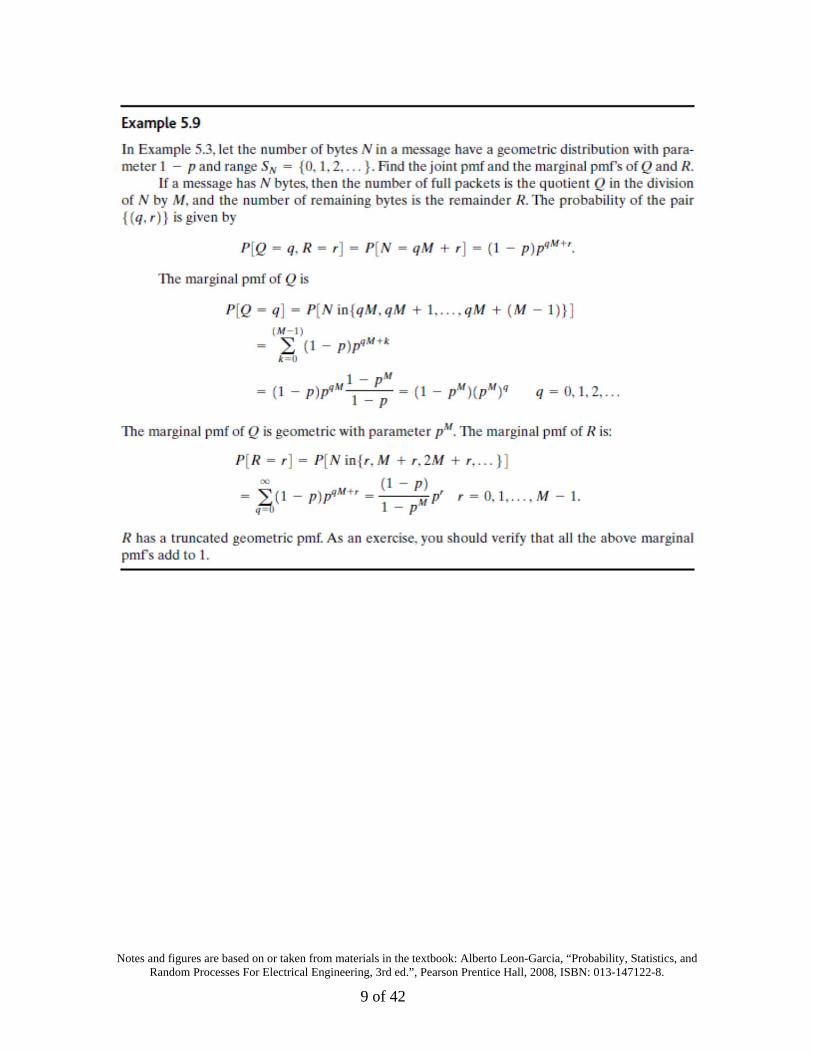
Embed Size (px)
Citation preview

Notes and figures are based on or taken from materials in the textbook: Alberto Leon-Garcia, “Probability, Statistics, and Random Processes For Electrical Engineering, 3rd ed.”, Pearson Prentice Hall, 2008, ISBN: 013-147122-8.
1 of 42
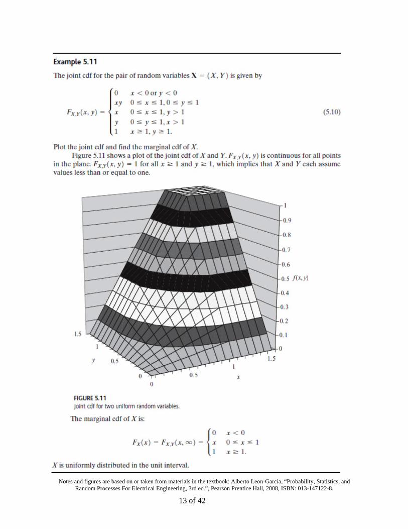
5. Pairs of Random Variable
Many random experiments involve several random variables. In some experiments a number of different quantities are measured. For example, the voltage signals at several points in a circuit at some specific time may be of interest. Other experiments involve the repeated measurement of a certain quantity such as the repeated measurement (“sampling”) of the amplitude of an audio or video signal that varies with time. In Chapter 4 we developed techniques for calculating the probabilities of events involving a single random variable in isolation. In this chapter, we extend the concepts already introduced to two random variables:
• We use the joint pmf, cdf, and pdf to calculate the probabilities of events that involve the joint behavior of two random variables;
• We use expected value to define joint moments that summarize the behavior of two random variables;
• We determine when two random variables are independent, and we quantify their degree of “correlation” when they are not independent;
• We obtain conditional probabilities involving a pair of random variables.
In a sense we have already covered all the fundamental concepts of probability and random variables, and we are “simply” elaborating on the case of two or more random variables. Nevertheless, there are significant analytical techniques that need to be learned, e.g., double summations of pmf’s and double integration of pdf’s, so we first discuss the case of two random variables in detail because we can draw on our geometric intuition. Chapter 6 considers the general case of vector random variables. Throughout these two chapters you should be mindful of the forest (fundamental concepts) and the trees (specific techniques)!
What we will see:
Joint Probability Mass and Density Functions – Marginal pmf and pdf as well
Cumulative Distribution Function
Conditional probability
Expected Value, Moments and Variance
New covariance
Notes and figures are based on or taken from materials in the textbook: Alberto Leon-Garcia, “Probability, Statistics, and Random Processes For Electrical Engineering, 3rd ed.”, Pearson Prentice Hall, 2008, ISBN: 013-147122-8.
2 of 42
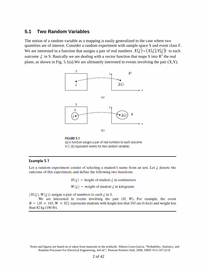
5.1 Two Random Variables
The notion of a random variable as a mapping is easily generalized to the case where two quantities are of interest. Consider a random experiment with sample space S and event class F. We are interested in a function that assigns a pair of real numbers YXX , to each outcome in S. Basically we are dealing with a vector function that maps S into R2 the real plane, as shown in Fig. 5.1(a).We are ultimately interested in events involving the pair (X,Y).
Notes and figures are based on or taken from materials in the textbook: Alberto Leon-Garcia, “Probability, Statistics, and Random Processes For Electrical Engineering, 3rd ed.”, Pearson Prentice Hall, 2008, ISBN: 013-147122-8.
3 of 42
The events involving a pair of random variables (X,Y) are specified by conditions that we are interested in and can be represented by regions in the plane.
To determine the probability that the pair X = (X,Y) is in some region B in the plane, we proceed as in Chapter 3 to find the equivalent event for B in the underlying sample space S:
BinYXBXA ,:1
The relationship between BXA 1 and B is shown in Fig. 5.1(b). If A is in F thenit has a probability assigned to it, and we obtain:
BinYXPAPBinXP ,:
The approach is identical to what we followed in the case of a single random variable. The only difference is that we are considering the joint behavior of X and Y that is induced by the underlying random experiment.
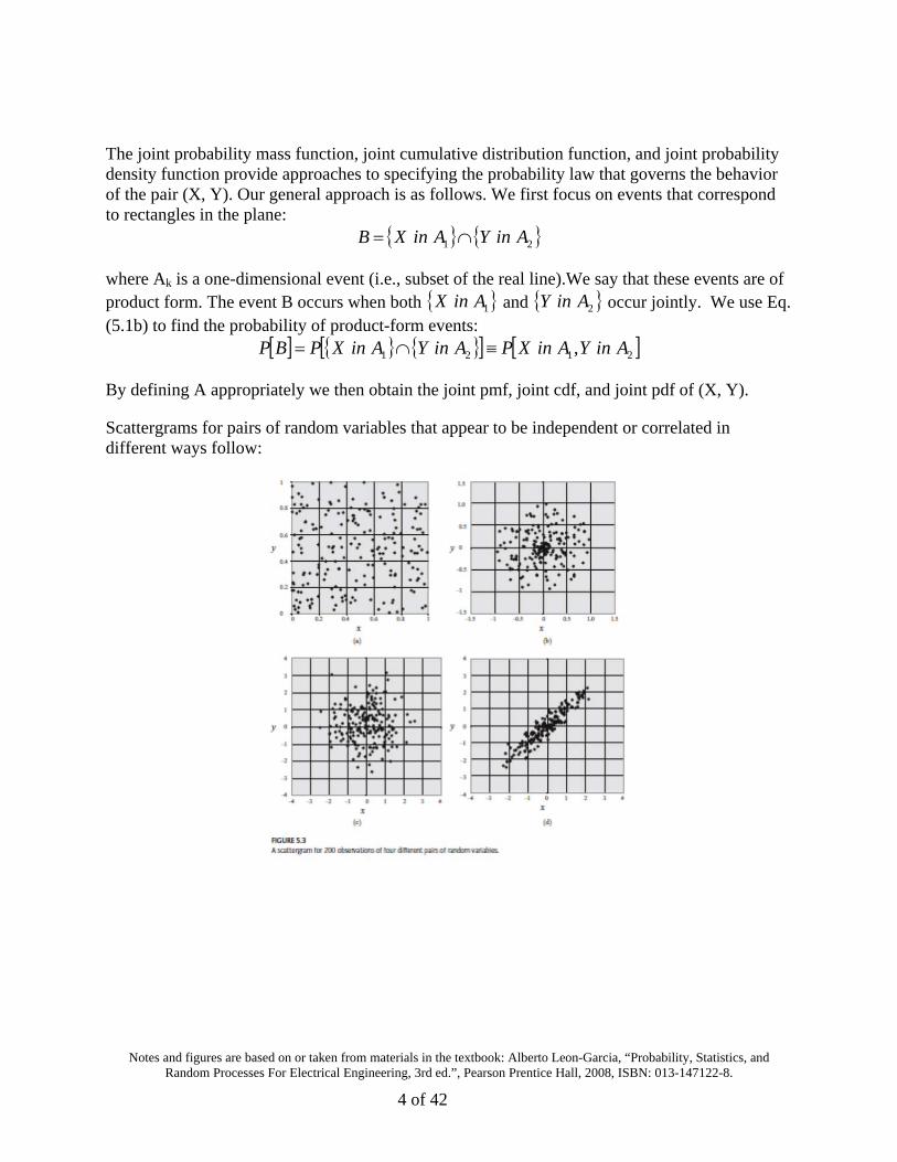
A scattergram can be used to deduce the joint behavior of two random variables. A scattergram plot simply places a dot at every observation pair (x, y) that results from performing the experiment that generates (X, Y).
Notes and figures are based on or taken from materials in the textbook: Alberto Leon-Garcia, “Probability, Statistics, and Random Processes For Electrical Engineering, 3rd ed.”, Pearson Prentice Hall, 2008, ISBN: 013-147122-8.
4 of 42
The joint probability mass function, joint cumulative distribution function, and joint probability density function provide approaches to specifying the probability law that governs the behavior of the pair (X, Y). Our general approach is as follows. We first focus on events that correspond to rectangles in the plane:
21 AinYAinXB
where Ak is a one-dimensional event (i.e., subset of the real line).We say that these events are of product form. The event B occurs when both 1AinX and 2AinY occur jointly. We use Eq. (5.1b) to find the probability of product-form events:
2121 , AinYAinXPAinYAinXPBP
By defining A appropriately we then obtain the joint pmf, joint cdf, and joint pdf of (X, Y).
Scattergrams for pairs of random variables that appear to be independent or correlated in different ways follow:

Notes and figures are based on or taken from materials in the textbook: Alberto Leon-Garcia, “Probability, Statistics, and Random Processes For Electrical Engineering, 3rd ed.”, Pearson Prentice Hall, 2008, ISBN: 013-147122-8.
5 of 42
5.2 Pairs of Discrete Random Variables
Let the vector random variable X = (X,Y) assume values from some countable set ,2,1,,2,1,,, kjyxS kjYX . The joint probability mass function of X specifies the
probabilities of the event yYxX :
yYxXPyxp YX ,,
yYxXPyxp YX ,,, , for 2, Ryx
The values of the pmf on the set YXS , provide the essential information:
kjkjYX yYxXPyxp ,,
kjkYX yYxXPyxp ,,, , for YXkj Syx ,,
There are several ways of showing the pmf graphically: (1) For small sample spaces we can present the pmf in the form of a table as shown in Fig. 5.5(a). (2) We can present the pmf using arrows of height kjYX yxp ,, placed at the points in the plane, as shown in Fig. 5.5(b), but this
can be difficult to draw. (3) We can place dots at the points ,2,1,,2,1,, kjyx kj and
label these with the corresponding pmf value as shown in Fig. 5.5(c)
Notes and figures are based on or taken from materials in the textbook: Alberto Leon-Garcia, “Probability, Statistics, and Random Processes For Electrical Engineering, 3rd ed.”, Pearson Prentice Hall, 2008, ISBN: 013-147122-8.
6 of 42
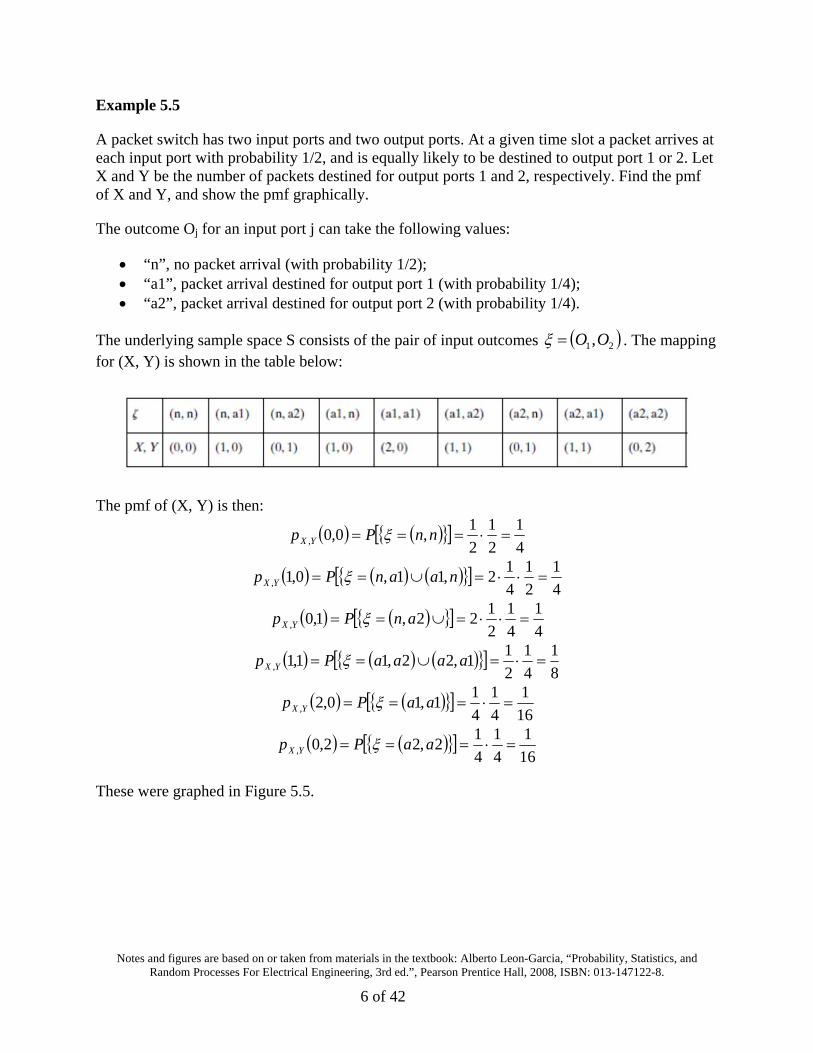
Example 5.5
A packet switch has two input ports and two output ports. At a given time slot a packet arrives at each input port with probability 1/2, and is equally likely to be destined to output port 1 or 2. Let X and Y be the number of packets destined for output ports 1 and 2, respectively. Find the pmf of X and Y, and show the pmf graphically.
The outcome Oj for an input port j can take the following values:
“n”, no packet arrival (with probability 1/2); “a1”, packet arrival destined for output port 1 (with probability 1/4); “a2”, packet arrival destined for output port 2 (with probability 1/4).
The underlying sample space S consists of the pair of input outcomes 21,OO . The mapping for (X, Y) is shown in the table below:
The pmf of (X, Y) is then:
4
1
2
1
2
1,0,0, nnPp YX
4
1
2
1
4
12,11,0,1, naanPp YX
4
1
4
1
2
122,1,0, anPp YX
8
1
4
1
2
11,22,11,1, aaaaPp YX
16
1
4
1
4
11,10,2, aaPp YX
16
1
4
1
4
12,22,0, aaPp YX
These were graphed in Figure 5.5.

Notes and figures are based on or taken from materials in the textbook: Alberto Leon-Garcia, “Probability, Statistics, and Random Processes For Electrical Engineering, 3rd ed.”, Pearson Prentice Hall, 2008, ISBN: 013-147122-8.
7 of 42
The probability of any event B is the sum of the pmf over the outcomes in B:
BinyxkYX
kj
yxpBinXP,
, ,
Frequently it is helpful to sketch the region that contains the points in B as shown, for example, in Fig. 5.6. When the event B is the entire sample space YXS , we have:
1,1 1
,
j kkYX yxp
The above graph corresponds to Example 5.6 of two loaded die.

Notes and figures are based on or taken from materials in the textbook: Alberto Leon-Garcia, “Probability, Statistics, and Random Processes For Electrical Engineering, 3rd ed.”, Pearson Prentice Hall, 2008, ISBN: 013-147122-8.
8 of 42
5.2.1 Marginal Probability Mass Function
The joint pmf of X provides the information about the joint behavior of X and Y. We are also interested in the probabilities of events involving each of the random variables in isolation. These can be found in terms of the marginal probability mass functions:
jjX xXPxp
anythingYxXPxp jjX ,
1
, ,k
kjYXjX yxpxp
and similarly
1
, ,j
kjYXkY yxpyp
The marginal pmf’s satisfy all the properties of one-dimensional pmf’s, and they supply the information required to compute the probability of events involving the corresponding random variable.
Notes and figures are based on or taken from materials in the textbook: Alberto Leon-Garcia, “Probability, Statistics, and Random Processes For Electrical Engineering, 3rd ed.”, Pearson Prentice Hall, 2008, ISBN: 013-147122-8.
9 of 42

Notes and figures are based on or taken from materials in the textbook: Alberto Leon-Garcia, “Probability, Statistics, and Random Processes For Electrical Engineering, 3rd ed.”, Pearson Prentice Hall, 2008, ISBN: 013-147122-8.
10 of 42
5.3 The Joint pdf of X and Y
In Chapter 3 we saw that semi-infinite intervals of the form ],( x are a basic building block
from which other one-dimensional events can be built. By defining the cdf xFX as the probability of ],( x , we were then able to express the probabilities of other events in terms of the cdf. In this section we repeat the above development for two-dimensional random variables.
A basic building block for events involving two-dimensional random variables is the semi-infinite rectangle defined by 11,:, yyxxyx as shown in Fig. 5.7. We also use the more
compact notation 11, yyxx to refer to this region. The joint cumulative distribution
function of X and Y is defined as the probability of the event 11 yYxX :
1111, ,, yYxXPyxF YX
The joint cdf satisfies the following properties.
(i) The joint cdf is a nondecreasing function of x and y:
22,11, ,, yxFyxF YXYX , if 21 xx and 21 yy
(ii) ( 0,, ,, xFyF YXYX and 1,, YXF
(iii) We obtain the marginal cumulative distribution functions by removing the constraint on one of the variables. The marginal cdf’s are the probabilities of the regions shown in Fig. 5.8:
xFxF XYX ,, and yFyF YYX ,,
(iv) The joint cdf is continuous from the “north” and from the “east,” that is,
yaFyxF YXYXax
,,lim ,,
and bxFyxF YXYXby
,,lim ,,
(v) The probability of the rectangle 2121 , yyyxxx is given by
11,21,12,22,2121 ,,,,, yxFyxFyxFyxFyyyxxxP YXYXYXYX
For property (v) note in Fig. 5.9(a) that
1112121 ,,, yyxXyyxXyyxxxB
11,12, ,, yxFyxFBP YXYX

Notes and figures are based on or taken from materials in the textbook: Alberto Leon-Garcia, “Probability, Statistics, and Random Processes For Electrical Engineering, 3rd ed.”, Pearson Prentice Hall, 2008, ISBN: 013-147122-8.
11 of 42
1112121 ,,, yyxXyyxXyyxxxB
11,12, ,, yxFyxFBP YXYX
In Fig. 5.9(b), note that
121221 ,, yyxxxyyxxxA
BPyxFyxFAP YXYX 21,22, ,,
Therefore,
11,12,21,22, ,,,, yxFyxFyxFyxFAP YXYXYXYX

Notes and figures are based on or taken from materials in the textbook: Alberto Leon-Garcia, “Probability, Statistics, and Random Processes For Electrical Engineering, 3rd ed.”, Pearson Prentice Hall, 2008, ISBN: 013-147122-8.
12 of 42
Notes and figures are based on or taken from materials in the textbook: Alberto Leon-Garcia, “Probability, Statistics, and Random Processes For Electrical Engineering, 3rd ed.”, Pearson Prentice Hall, 2008, ISBN: 013-147122-8.
13 of 42

Notes and figures are based on or taken from materials in the textbook: Alberto Leon-Garcia, “Probability, Statistics, and Random Processes For Electrical Engineering, 3rd ed.”, Pearson Prentice Hall, 2008, ISBN: 013-147122-8.
14 of 42

Notes and figures are based on or taken from materials in the textbook: Alberto Leon-Garcia, “Probability, Statistics, and Random Processes For Electrical Engineering, 3rd ed.”, Pearson Prentice Hall, 2008, ISBN: 013-147122-8.
15 of 42
5.3.1 Random Variables That Differ in Type
In some problems it is necessary to work with joint random variables that differ in type, that is, one is discrete and the other is continuous. Usually it is rather clumsy to work with the joint cdf, and so it is preferable to work with either yYkXP , or 21, yYykXP . These probabilities are sufficient to compute the joint cdf should we have to.

Notes and figures are based on or taken from materials in the textbook: Alberto Leon-Garcia, “Probability, Statistics, and Random Processes For Electrical Engineering, 3rd ed.”, Pearson Prentice Hall, 2008, ISBN: 013-147122-8.
16 of 42
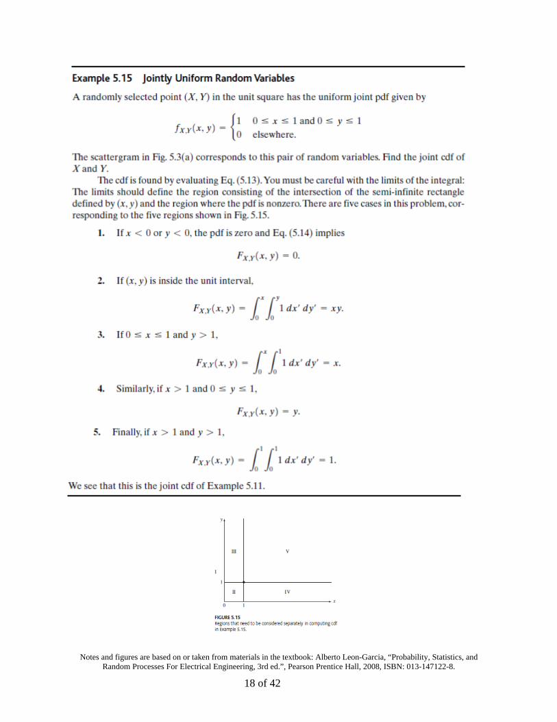
5.4 The Joint cdf of Two Continuous Random Variables
The joint cdf allows us to compute the probability of events that correspond to “rectangular” shapes in the plane. To compute the probability of events corresponding to regions other than rectangles, we note that any reasonable shape (i.e., disk, polygon, or half-plane) can be approximated by the union of disjoint infinitesimal rectangles, For example, Fig. 5.12 shows how the events 1 YXA and 122 YXA are approximated by rectangles of infinitesimal width. The probability of such events can therefore be approximated by the sum of the probabilities of infinitesimal rectangles, and if the cdf is sufficiently smooth, the probability of each rectangle can be expressed in terms of a density function:
Byx
kjYXj k
kj
kj
yxyxfBPBP,
,, ,
As x and y approach zero, the above equation becomes an integral of a probability density function over the region B.
We say that the random variables X and Y are jointly continuous if the probabilities of events involving (X, Y) can be expressed as an integral of a probability density function. In other words, there is a nonnegative function yXf YX ,, called the joint probability density function,
that is defined on the real plane such that for every event B, a subset of the plane,
''',', B
YX dydxyxfBinXP

Notes and figures are based on or taken from materials in the textbook: Alberto Leon-Garcia, “Probability, Statistics, and Random Processes For Electrical Engineering, 3rd ed.”, Pearson Prentice Hall, 2008, ISBN: 013-147122-8.
17 of 42
The joint cdf can be obtained in terms of the joint pdf of jointly continuous random variables by integrating over the semi-infinite rectangle defined by (x, y):
x y
YXYX dydxyxfyxF ,, ,,
It then follows that if X and Y are jointly continuous random variables, then the pdf can be obtained from the cdf by differentiation:
yxFyx
yxf YXYX ,, ,
2
,
Note that if X and Y are not jointly continuous, then it is possible that the above partial derivative does not exist. In particular, if the yxF YX ,, is discontinuous or if its partial
derivatives are discontinuous, then the joint pdf as defined by Eq. (5.14) will not exist.
The marginal pdf’s xf X and yfY are obtained by taking the derivative of the corresponding
marginal cdf’s, ,, xFxF YXX and yFyF YXY ,, . Thus
''',', dxdyyxfdx
dxf
x
YXX
'',, dyyxfxf YXX
Similarly
',', dxyxfyf YXY
Thus the marginal pdf’s are obtained by integrating out the variables that are not of interest.
Notes and figures are based on or taken from materials in the textbook: Alberto Leon-Garcia, “Probability, Statistics, and Random Processes For Electrical Engineering, 3rd ed.”, Pearson Prentice Hall, 2008, ISBN: 013-147122-8.
18 of 42

Notes and figures are based on or taken from materials in the textbook: Alberto Leon-Garcia, “Probability, Statistics, and Random Processes For Electrical Engineering, 3rd ed.”, Pearson Prentice Hall, 2008, ISBN: 013-147122-8.
19 of 42

Notes and figures are based on or taken from materials in the textbook: Alberto Leon-Garcia, “Probability, Statistics, and Random Processes For Electrical Engineering, 3rd ed.”, Pearson Prentice Hall, 2008, ISBN: 013-147122-8.
20 of 42
Example 5.18 Jointly Gaussian Random Variables
The joint pdf of X and Y, shown in Fig. 5.17, is
2
22
2, 12
2exp
12
1,
yyxxyxf YX , yx,
We say that X and Y are jointly Gaussian. Find the marginal pdf’s.
The marginal pdf of X is found by integrating yxf YX ,, over y:
dy
yyxxxf X 2
22
2 12
2exp
12
1
dy
yxyxxf X 2
2
2
2
2 12
2exp
12exp
12
1
We complete the square of the argument of the exponent by adding and subtracting 22 x . Therefore
dy
xyxyxxxf X 2
222
2
222
2 12
2exp
12exp
12
1
dy
xyxxf X 2
2
2
2
12exp
12
1
2exp
2
1
2exp
2
1 2xxf X
where we have noted that the last integral equals one since its integrand is a Gaussian pdf with mean x and variance 21 . The marginal pdf of X is therefore a one-dimensional Gaussian
pdf with mean 0 and variance 1. From the symmetry of yxf YX ,, in x and y, we conclude that
the marginal pdf of Y is also a one-dimensional Gaussian pdf with zero mean and unit variance.

Notes and figures are based on or taken from materials in the textbook: Alberto Leon-Garcia, “Probability, Statistics, and Random Processes For Electrical Engineering, 3rd ed.”, Pearson Prentice Hall, 2008, ISBN: 013-147122-8.
21 of 42

Notes and figures are based on or taken from materials in the textbook: Alberto Leon-Garcia, “Probability, Statistics, and Random Processes For Electrical Engineering, 3rd ed.”, Pearson Prentice Hall, 2008, ISBN: 013-147122-8.
22 of 42
5.5 Independence of Two Random Variables
X and Y are independent random variables if any event 1A defined in terms of X is independent
of any 2A event defined in terms of Y; that is,
2121 , AinYPAinXPAinYAinXP
Suppose that X and Y are a pair of discrete random variables, and suppose we are interested in the probability of the event 21 AA where 1A involves only X and 2A involves only Y. In
particular, if X and Y are independent, then 1A and 2A are independent events. If we let
jxXA 1 and kyYA 2 then the independence of X and Y implies that
kjkjYX yYxXPyxp ,,,
kjkjYX yYPxXPyxp ,,
kYjXkjYX ypxpyxp ,,
Therefore, if X and Y are independent discrete random variables, then the joint pmf is equal to the product of the marginal pmf’s.
Now suppose that we don’t know if X and Y are independent, but we do know that the pmf satisfies the above equation. Let 21 AAA be a product-form event as above, then
1 2
,,AinX AinY
kjYX yxpAP
1 2AinX AinY
kYjX ypxpAP
1 2AinX AinY
kYjX ypxpAP
21 APAPAP
which implies 1A that and 2A are independent events. Therefore, if the joint pmf of X and Y equals the product of the marginal pmf’s, then X and Y are independent. We have just proved that the statement “X and Y are independent” is equivalent to the statement “the joint pmf is equal to the product of the marginal pmf’s.” In mathematical language, we say, the “discrete random variables X and Y are independent if and only if the joint pmf is equal to the product of the marginal pmf’s for all kj yx , .”
Notes and figures are based on or taken from materials in the textbook: Alberto Leon-Garcia, “Probability, Statistics, and Random Processes For Electrical Engineering, 3rd ed.”, Pearson Prentice Hall, 2008, ISBN: 013-147122-8.
23 of 42
In general, it can be shown that the random variables X and Y are independent if and only if their joint cdf is equal to the product of its marginal cdf’s:
yFxFyxF YXYX ,, , for all x and y.
Similarly, if X and Y are jointly continuous, then X and Y are independent if and only if their joint pdf is equal to the product of the marginal pdf’s:
yfxfyxf YXYX ,, , for all x and y.
Joint Gaussian pdf from Example 5.18 … notice the “correlation coefficient”
2
22
2, 12
2exp
12
1,
yyxxyxf YX , yx,
Note also that:
If X and Y are independent random variables, then the random variables defined by any pair of functions g(X) and h(Y) are also independent.
Notes and figures are based on or taken from materials in the textbook: Alberto Leon-Garcia, “Probability, Statistics, and Random Processes For Electrical Engineering, 3rd ed.”, Pearson Prentice Hall, 2008, ISBN: 013-147122-8.
24 of 42
5.6 Joint Moments and Expected Value of a Function of Two Random Variables
The expected value of X identifies the center of mass of the distribution of X. The variance, which is defined as the expected value of 2mX provides a measure of the spread of the distribution. In the case of two random variables we are interested in how X and Y vary together. In particular, we are interested in whether the variation of X and Y are correlated. For example, if X increases does Y tend to increase or to decrease? The joint moments of X and Y, which are defined as expected values of functions of X and Y, provide this information.
5.6.1 Expected Values of a Function of Two Random Variables
The problem of finding the expected value of a function of two or more random variables is similar to that of finding the expected value of a function of a single random variable. It can be shown that the expected value of yxgZ , can be found using the following expressions:
dydxyxfyxgZE YX ,, , , X,Y jointly continuous
or
j k
kjYXkj yxfyxgZE ,, , , X,Y discrete
Example 5.24 Sum of Random Variables
Let Z = X + Y. Let Find E[Z]. YXEZE
dydxyxfyxZE YX ,,
dydxyxfydydxyxfxZE YXYX ,, ,,
dyyfydxxfxZE YX
YEXEZE
Thus the expected value of the sum of two random variables is equal to the sum of the individual expected values. Note that X and Y need not be independent.
Note that the random variables do not have to be independent.
Notes and figures are based on or taken from materials in the textbook: Alberto Leon-Garcia, “Probability, Statistics, and Random Processes For Electrical Engineering, 3rd ed.”, Pearson Prentice Hall, 2008, ISBN: 013-147122-8.
25 of 42
Example 5.25 Product of Functions of Independent Random Variables
Suppose that X and Y are independent random variables, and let YgXgYXg 21, .
Find YgXgEYXgE 21,
dydxyxfYgXgYgXgE YX ,,2121
If the variables are independent,
dydxyfxfYgXgYgXgE YX2121
dyyfYgdxxfXgYgXgE YX 2121
YgEXgEYgXgE 2121
5.6.2 Joint Moments, Correlation and Covariance
The joint moments of two random variables X and Y summarize information about their joint behavior. The jkth joint moment of X and Y is defined by
dydxyxfyxYXE YXkjkj ,, X,Y jointly continuous
or
j k
kjYXkjkj yxfyxYXE ,, , X,Y discrete
If j=0 we obtain the moments of Y, and if k=0 we obtain the moments of X.
In electrical engineering, it is customary to call the j=k=1 moment, E[XY], the correlation of X and Y. If E[XY]=0 then we say that X and Y are orthogonal
The jkth central moment of X and Y is defined as the joint moment of the centered random variables XEX and YEY :
kj YEYXEXE
Note that j=2 with k=0 gives VAR(X) and j=0 with k=2 gives VAR(Y).

Notes and figures are based on or taken from materials in the textbook: Alberto Leon-Garcia, “Probability, Statistics, and Random Processes For Electrical Engineering, 3rd ed.”, Pearson Prentice Hall, 2008, ISBN: 013-147122-8.
26 of 42
The covariance of X and Y is defined as the j=k=1 central moment: YEYXEXEYXCOV ,
The following form for COV(X, Y) is sometimes more convenient to work with YEXEYEXXEYYXEYXCOV ,
YEXEYEXEYXEYXCOV 2,
YEXEYXEYXCOV ,
Note that YXEYXCOV , if either of the random variables has a zero mean.
Let’s see how the covariance measures the correlation between X and Y. The covariance measures the deviation from XEmX and YEmY . If a positive value of XmX tends to
be accompanied by a positive values of YmY and negative XmX tend to be accompanied by
negative YmY ; then YX mYmXEYXCOV , will tend to be a positive value, and its expected value, COV(X,Y), will be positive.
On the other hand, if XmX and YmY tend to have opposite signs, then COV(X,Y) will be negative. A scattergram for this case would have observation points cluster along a line of negative slope. Finally if and sometimes have the same sign and sometimes have opposite signs, then COV(X,Y) will be close to zero.
Multiplying either X or Y by a large number will increase the covariance, so we need to normalize the covariance to measure the correlation in an absolute scale. The correlation coefficient of X and Y is defined by
YXYX
YX
YEXEYXEYXCOV
,
,
where 11 , YX
Notes and figures are based on or taken from materials in the textbook: Alberto Leon-Garcia, “Probability, Statistics, and Random Processes For Electrical Engineering, 3rd ed.”, Pearson Prentice Hall, 2008, ISBN: 013-147122-8.
27 of 42
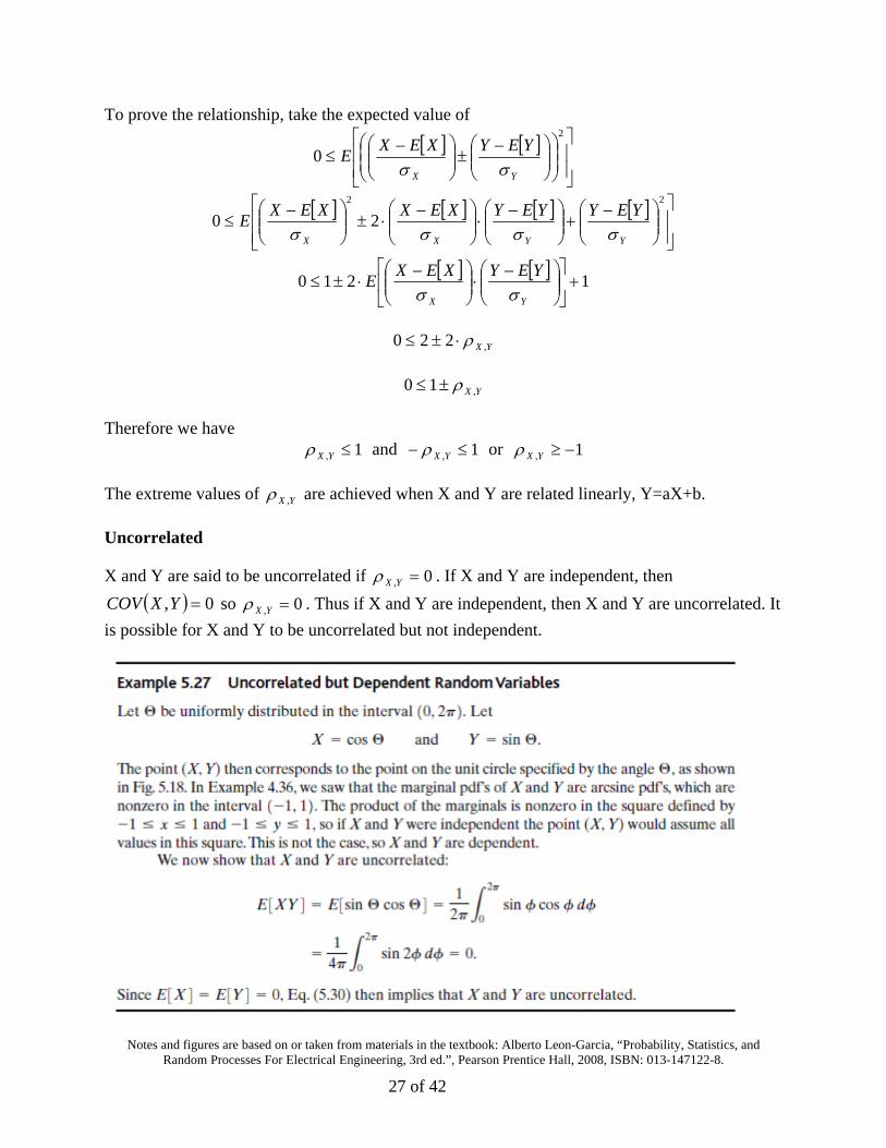
To prove the relationship, take the expected value of
2
0YX
YEYXEXE
22
20YYXX
YEYYEYXEXXEXE
1210
YX
YEYXEXE
YX ,220
YX ,10
Therefore we have 1, YX and 1, YX or 1, YX
The extreme values of YX , are achieved when X and Y are related linearly, Y=aX+b.
Uncorrelated
X and Y are said to be uncorrelated if 0, YX . If X and Y are independent, then
0, YXCOV so 0, YX . Thus if X and Y are independent, then X and Y are uncorrelated. It
is possible for X and Y to be uncorrelated but not independent.
Notes and figures are based on or taken from materials in the textbook: Alberto Leon-Garcia, “Probability, Statistics, and Random Processes For Electrical Engineering, 3rd ed.”, Pearson Prentice Hall, 2008, ISBN: 013-147122-8.
28 of 42
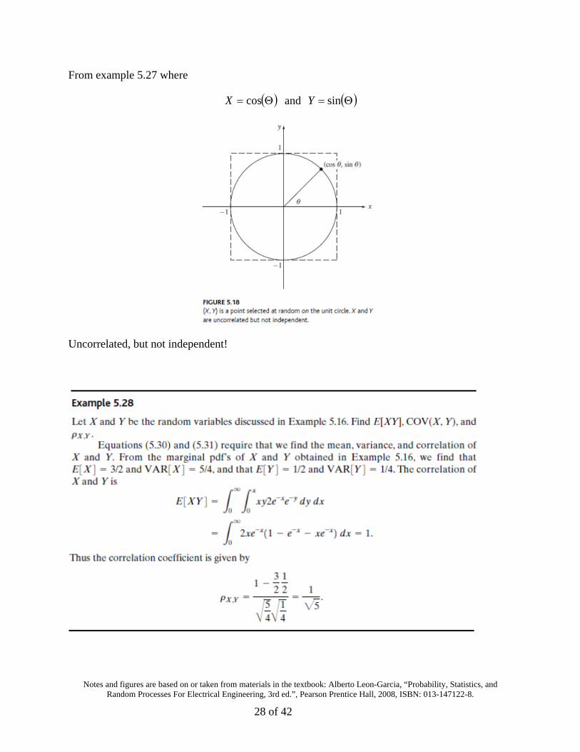
From example 5.27 where
cosX and sinY
Uncorrelated, but not independent!
Notes and figures are based on or taken from materials in the textbook: Alberto Leon-Garcia, “Probability, Statistics, and Random Processes For Electrical Engineering, 3rd ed.”, Pearson Prentice Hall, 2008, ISBN: 013-147122-8.
29 of 42
5.7 Conditional Probability and Conditional Expectation
Many random variables of practical interest are not independent:The output Y of a communication channel must depend on the input X in order to convey information; consecutive samples of a waveform that varies slowly are likely to be close in value and hence are not independent. In this section we are interested in computing the probability of events concerning the random variable Y given that we know xX . We are also interested in the expected value of Y given xX . We show that the notions of conditional probability and conditional expectation are extremely useful tools in solving problems, even in situations where we are only concerned with one of the random variables.
5.7.1 Conditional Probability
The definition of conditional probability in Section 2.4 allows us to compute the probability that Y is in A given that we know that xX :
xXP
xXAinYPxXAinYP
,
| , for 0 xXP
Case 1: X Is a Discrete Random Variable
For X and Y discrete random variables, the conditional pmf of Y given xX is defined by:
xp
yxp
xXP
xXyYPxypxXyYP
X
YXY
,,|| ,
The conditional pmf satisfies all the properties of a pmf, that is, it assigns nonnegative values to every y and these values add to 1.
If X and Y are independent,
ypxp
xpypxyp Y
X
XYY
|
Other relationships
xpxypyxp XYYX |,,
ypyxpyxp YYYX |,,
Notes and figures are based on or taken from materials in the textbook: Alberto Leon-Garcia, “Probability, Statistics, and Random Processes For Electrical Engineering, 3rd ed.”, Pearson Prentice Hall, 2008, ISBN: 013-147122-8.
30 of 42
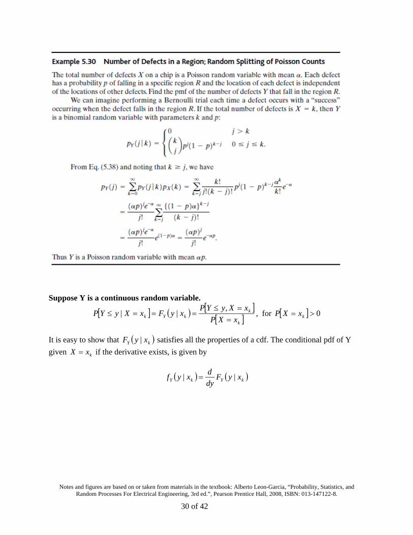
Suppose Y is a continuous random variable.
k
kkYk xXP
xXyYPxyFxXyYP
,
|| , for 0 kxXP
It is easy to show that kY xyF | satisfies all the properties of a cdf. The conditional pdf of Y
given kxX if the derivative exists, is given by
kYkY xyFdy
dxyf ||
Notes and figures are based on or taken from materials in the textbook: Alberto Leon-Garcia, “Probability, Statistics, and Random Processes For Electrical Engineering, 3rd ed.”, Pearson Prentice Hall, 2008, ISBN: 013-147122-8.
31 of 42
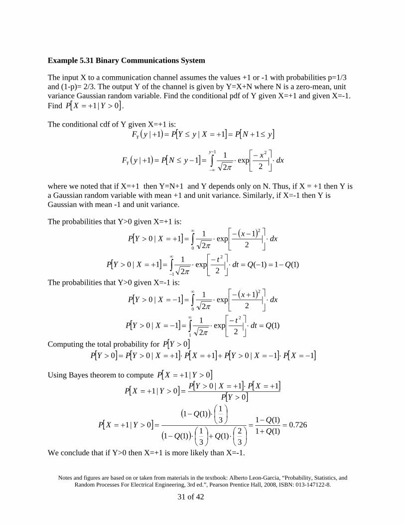
Example 5.31 Binary Communications System
The input X to a communication channel assumes the values +1 or -1 with probabilities p=1/3 and (1-p)= 2/3. The output Y of the channel is given by Y=X+N where N is a zero-mean, unit variance Gaussian random variable. Find the conditional pdf of Y given X=+1 and given X=-1. Find 0|1 YXP .
The conditional cdf of Y given X=+1 is: yNPXyYPyFY 11|1|
1 2
2exp
2
111|
y
Y dxx
yNPyF
where we noted that if X=+1 then Y=N+1 and Y depends only on N. Thus, if X = +1 then Y is a Gaussian random variable with mean +1 and unit variance. Similarly, if X=-1 then Y is Gaussian with mean -1 and unit variance.
The probabilities that Y>0 given X=+1 is:
0
2
2
1exp
2
11|0 dx
xXYP
)1(1)1(2
exp2
11|0
1
2
QQdtt
XYP
The probabilities that Y>0 given X=-1 is:
0
2
2
1exp
2
11|0 dx
xXYP
)1(2
exp2
11|0
1
2
Qdtt
XYP
Computing the total probability for 0YP
11|011|00 XPXYPXPXYPYP
Using Bayes theorem to compute 0|1 YXP
0
11|00|1
YP
XPXYPYXP
726.0
)1(1
)1(1
3
2)1(
3
1)1(1
3
1)1(1
0|1
Q
Q
Q
YXP
We conclude that if Y>0 then X=+1 is more likely than X=-1.

Notes and figures are based on or taken from materials in the textbook: Alberto Leon-Garcia, “Probability, Statistics, and Random Processes For Electrical Engineering, 3rd ed.”, Pearson Prentice Hall, 2008, ISBN: 013-147122-8.
32 of 42
Find 0|1 YXP .
The probabilities that Y < 0 given X=-1 is:
0 2
2
1exp
2
11|0 dx
xXYP
)1(12
exp2
11|0
1 2
Qdtt
XYP
The probabilities that Y<0 given X=+1 is:
0 2
2
1exp
2
11|0 dx
xXYP
1112
exp2
11|0
1 2
QQdtt
XYP
Computing the total probability for 0YP
11|011|00 XPXYPXPXYPYP
Using Bayes theorem to compute 0|1 YXP
0
11|00|1
YP
XPXYPYXP
848.0
)1(2
)1(22
3
1)1(
3
2)1(1
3
2)1(1
0|1
Q
Q
Q
YXP
We conclude that if Y<0 then X=-1 is more likely than X=+1.

Notes and figures are based on or taken from materials in the textbook: Alberto Leon-Garcia, “Probability, Statistics, and Random Processes For Electrical Engineering, 3rd ed.”, Pearson Prentice Hall, 2008, ISBN: 013-147122-8.
33 of 42
Case 2: X Is a Continuous Random Variable
If X is a continuous random variable, then 0 kxXP so Eq. (5.33) is undefined for all x. If
X and Y have a joint pdf that is continuous and nonzero over some region of the plane, we define the conditional cdf of Y given X=x by the following limiting procedure:
hXxyFxyF Yh
Y
|lim|0
The conditional cdf on the right side is
hXxP
hXxyYPhXxyFY
,|
hxf
dyhyxf
hXxyFX
y
YX
Y
'',
|,
As we let h approach zero,
xf
dyyxf
xyFX
y
YX
Y
'',
|,
The conditional pdf of Y given X=x is then:
xf
yxfxyf
X
YXY
,| ,
This example is all messed up ….
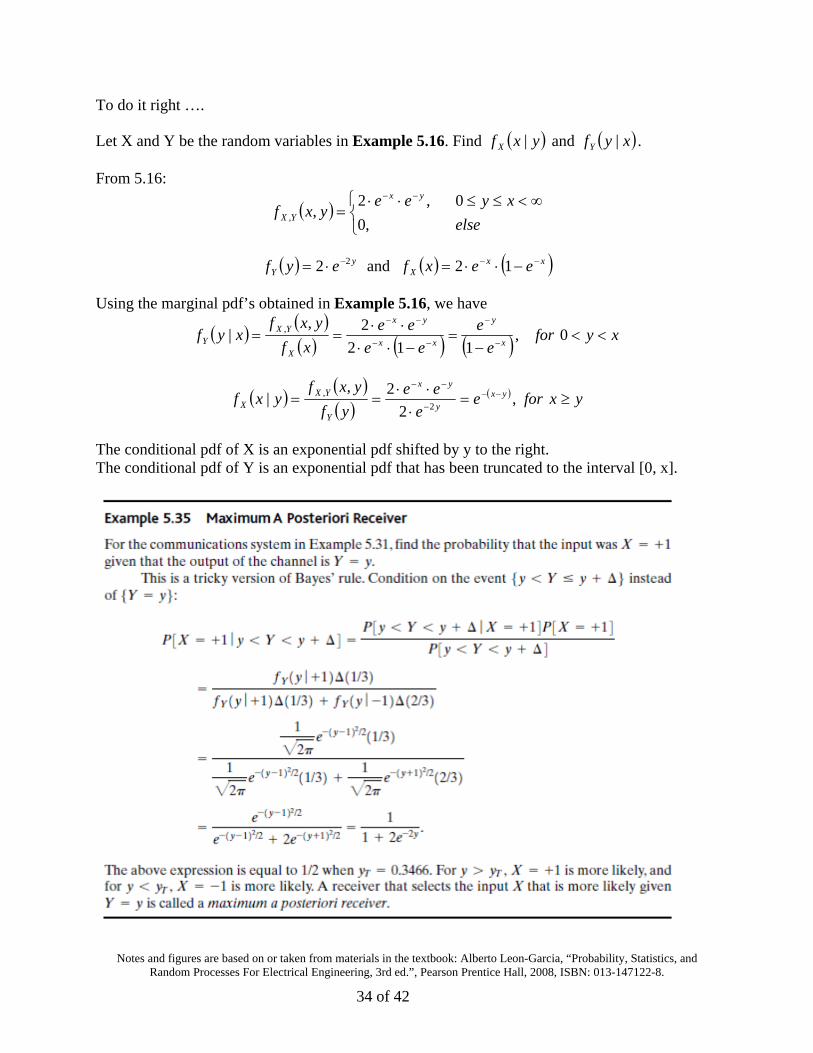
Notes and figures are based on or taken from materials in the textbook: Alberto Leon-Garcia, “Probability, Statistics, and Random Processes For Electrical Engineering, 3rd ed.”, Pearson Prentice Hall, 2008, ISBN: 013-147122-8.
34 of 42
To do it right ….
Let X and Y be the random variables in Example 5.16. Find yxf X | and xyfY | .
From 5.16:
else
xyeeyxf
yx
YX,0
0,2,,
yY eyf 22 and xx
X eexf 12
Using the marginal pdf’s obtained in Example 5.16, we have
xyfor
e
e
ee
ee
xf
yxfxyf
x
y
xx
yx
X
YXY
0,112
2,| ,
yxforee
ee
yf
yxfyxf yx
y
yx
Y
YXX
,2
2,|
2
,
The conditional pdf of X is an exponential pdf shifted by y to the right. The conditional pdf of Y is an exponential pdf that has been truncated to the interval [0, x].
Notes and figures are based on or taken from materials in the textbook: Alberto Leon-Garcia, “Probability, Statistics, and Random Processes For Electrical Engineering, 3rd ed.”, Pearson Prentice Hall, 2008, ISBN: 013-147122-8.
35 of 42
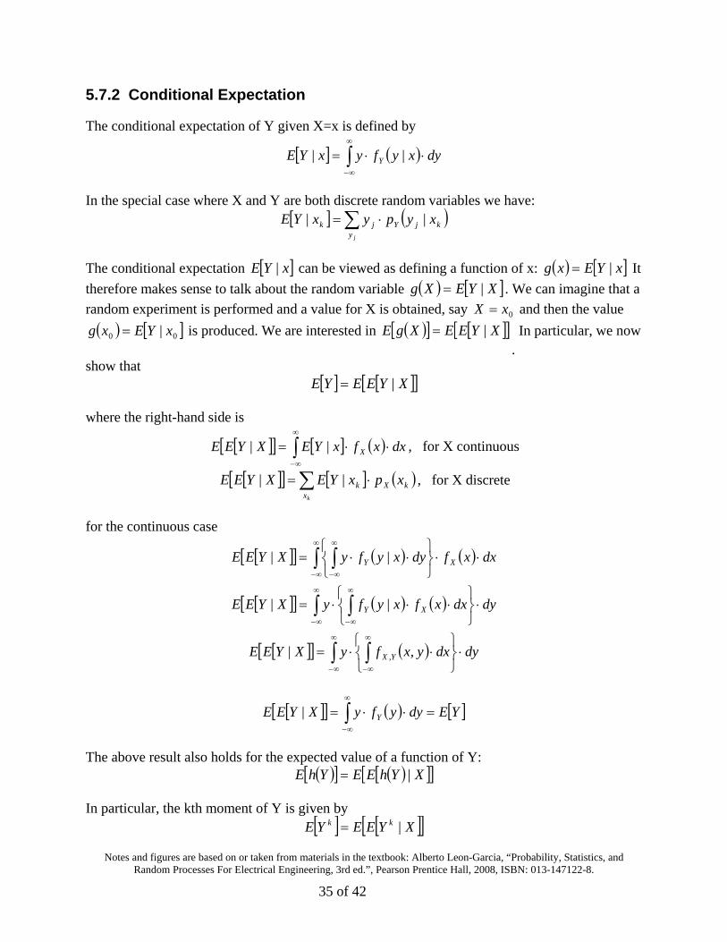
5.7.2 Conditional Expectation
The conditional expectation of Y given X=x is defined by
dyxyfyxYE Y ||
In the special case where X and Y are both discrete random variables we have:
jykjYjk xypyxYE ||
The conditional expectation xYE | can be viewed as defining a function of x: xYExg |
It
therefore makes sense to talk about the random variable XYEXg | . We can imagine that a
random experiment is performed and a value for X is obtained, say 0xX and then the value
00 | xYExg is produced. We are interested in XYEEXgE |
. In particular, we now
show that XYEEYE |
where the right-hand side is
dxxfxYEXYEE X|| , for X continuous
kx
kXk xpxYEXYEE || , for X discrete
for the continuous case
dxxfdyxyfyXYEE XY ||
dydxxfxyfyXYEE XY
||
dydxyxfyXYEE YX
,| ,
YEdyyfyXYEE Y
|
The above result also holds for the expected value of a function of Y: XYhEEYhE |
In particular, the kth moment of Y is given by XYEEYE kk |

Notes and figures are based on or taken from materials in the textbook: Alberto Leon-Garcia, “Probability, Statistics, and Random Processes For Electrical Engineering, 3rd ed.”, Pearson Prentice Hall, 2008, ISBN: 013-147122-8.
36 of 42
Notes and figures are based on or taken from materials in the textbook: Alberto Leon-Garcia, “Probability, Statistics, and Random Processes For Electrical Engineering, 3rd ed.”, Pearson Prentice Hall, 2008, ISBN: 013-147122-8.
37 of 42
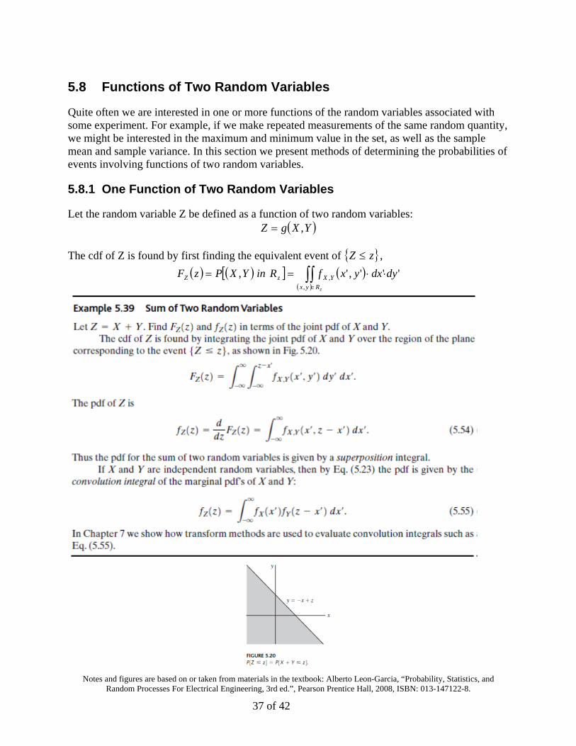
5.8 Functions of Two Random Variables
Quite often we are interested in one or more functions of the random variables associated with some experiment. For example, if we make repeated measurements of the same random quantity, we might be interested in the maximum and minimum value in the set, as well as the sample mean and sample variance. In this section we present methods of determining the probabilities of events involving functions of two random variables.
5.8.1 One Function of Two Random Variables
Let the random variable Z be defined as a function of two random variables: YXgZ ,
The cdf of Z is found by first finding the equivalent event of zZ ,
zRyx
YXzZ dydxyxfRinYXPzF,
, ''',',
Notes and figures are based on or taken from materials in the textbook: Alberto Leon-Garcia, “Probability, Statistics, and Random Processes For Electrical Engineering, 3rd ed.”, Pearson Prentice Hall, 2008, ISBN: 013-147122-8.
38 of 42
5.8.2 Transformations of Two Random Variables
Let X and Y be random variables associated with some experiment, and let the random variables
1Z and 2Z be defined by two functions of YX , :
YXgZ ,11 and YXgZ ,22
We now consider the problem of finding the joint cdf and pdf of 1Z and 2Z .
The joint cdf of 1Z and 2Z at the point is equal to the probability of the region of x where
kk zyxg , for k=1,2:
221121, ,,,,21
zYXgzYXgPzzF ZZ
If X, Y have a joint pdf, then
kk zgyx
YXZZ dydxyxfzzF:,
,21, ''',',21

Notes and figures are based on or taken from materials in the textbook: Alberto Leon-Garcia, “Probability, Statistics, and Random Processes For Electrical Engineering, 3rd ed.”, Pearson Prentice Hall, 2008, ISBN: 013-147122-8.
39 of 42
5.8.3 pdf of Linear Transformations
The joint pdf of Z can be found directly in terms of the joint pdf of X by finding the equivalent events of infinitesimal rectangles.We consider the linear transformation of two random variables:
Denote the above matrix by A. We will assume that A has an inverse, that is, it has determinant 0 cbea so each point (v, w) has a unique corresponding point (x, y) obtained from
Consider the infinitesimal rectangle shown in Fig. 5.23. The points in this rectangle are mapped into the parallelogram shown in the figure. The infinitesimal rectangle and the parallelogram are equivalent events, so their probabilities must be equal. Thus
dPwvfdydxyxf WVYX ,, ,,
where dP is the area of the parallelogram. The joint pdf of V and W is thus given by
dydx
dP
yxfwvf YX
WV
,, ,
,
where x and y are related to (v,w) by Eq. (5.58). Equation (5.59) states that the joint pdf of V and W at (v,w) is the pdf of X and Y at the corresponding point (x, y), but rescaled by the “stretch factor” dP/dx dy. It can be shown that dydxcbeadP , so the “stretch factor” is
Acbea
dydx
dydxcbea
dydx
dP
where A is the determinant of A.
The above result can be written compactly using matrix notation. Let the vector Z be
XAZ
where A is an n x n invertible matrix. The joint pdf of Z is then
A
zAfzf X
Z
1

Notes and figures are based on or taken from materials in the textbook: Alberto Leon-Garcia, “Probability, Statistics, and Random Processes For Electrical Engineering, 3rd ed.”, Pearson Prentice Hall, 2008, ISBN: 013-147122-8.
40 of 42
5.9 Pairs of Jointly Gaussian Random Variables
Left to be read by the students ….

Notes and figures are based on or taken from materials in the textbook: Alberto Leon-Garcia, “Probability, Statistics, and Random Processes For Electrical Engineering, 3rd ed.”, Pearson Prentice Hall, 2008, ISBN: 013-147122-8.
41 of 42
Summary
• The joint statistical behavior of a pair of random variables X and Y is specified by the joint cumulative distribution function, the joint probability mass function, or the joint probability density function. The probability of any event involving the joint behavior of these random variables can be computed from these functions.
• The statistical behavior of individual random variables from X is specified by the marginal cdf, marginal pdf, or marginal pmf that can be obtained from the joint cdf, joint pdf, or joint pmf of X.
• Two random variables are independent if the probability of a product-form event is equal to the product of the probabilities of the component events. Equivalent conditions for the independence of a set of random variables are that the joint cdf, joint pdf, or joint pmf factors into the product of the corresponding marginal functions.
• The covariance and the correlation coefficient of two random variables are measures of the linear dependence between the random variables.
• If X and Y are independent, then X and Y are uncorrelated, but not vice versa. If X and Y are jointly Gaussian and uncorrelated, then they are independent.
• The statistical behavior of X, given the exact values of X or Y, is specified by the conditional cdf, conditional pmf, or conditional pdf. Many problems lend themselves to a solution that involves conditioning on the value of one of the random variables. In these problems, the expected value of random variables can be obtained by conditional expectation.
• The joint pdf of a pair of jointly Gaussian random variables is determined by the means, variances, and covariance. All marginal pdf’s and conditional pdf’s are also Gaussian pdf’s.
• Independent Gaussian random variables can be generated by a transformation of uniform random variables.

Notes and figures are based on or taken from materials in the textbook: Alberto Leon-Garcia, “Probability, Statistics, and Random Processes For Electrical Engineering, 3rd ed.”, Pearson Prentice Hall, 2008, ISBN: 013-147122-8.
42 of 42
CHECKLIST OF IMPORTANT TERMS Central moments of X and Y
Conditional cdf
Conditional expectation
Conditional pdf
Conditional pmf
Correlation of X and Y
Covariance X and Y
Independent random variables
Joint cdf
Joint moments of X and Y
Joint pdf
Joint pmf
Jointly continuous random variables
Jointly Gaussian random variables
Linear transformation
Marginal cdf
Marginal pdf
Marginal pmf
Orthogonal random variables
Product-form event
Uncorrelated random variables


![E DATA PROJECTOR XJ-A130/XJ-A135 XJ-A140/XJ-A145 XJ … · 2010-04-28 · 3. To restore the audio, press the [VOLUME] key again. Adjusting the Volume Level. 15 The following three](https://img.pdfslide.us/doc/110x75/5f36bb595cbf8553ed190941/e-data-projector-xj-a130xj-a135-xj-a140xj-a145-xj-2010-04-28-3-to-restore-the.jpg)