5 Interconnection Networks 5.1 INTRODUCTION Networking strategy was originally employed in the 1950's by the telephone industry as a means of reducing the time required for a call to go through. Similarly, the computer industry employs networking strategy to provide fast communication between computer subparts, particularly with regard to parallel machines. The performance requirements of many applications, such as weather prediction, signal processing, radar tracking, and image processing, far exceed the capabilities of single-processor architectures. Parallel machines break a single problem down into parallel tasks that are performed concurrently, reducing significantly the application processing time. Any parallel system that employs more than one processor per application program must be designed to allow its processors to communicate efficiently; otherwise, the advantages of parallel processing may be negated by inefficient communication. This fact emphasizes the importance of interconnection networks to overall parallel system performance. In many proposed or existing parallel processing architectures, an interconnection network is used to realize transportation of data between processors or between processors and memory modules. This chapter deals with several aspects of the networks used in modern (and theoretical) computers. After classifying various network structures, some of the most well known networks are discussed, along with a list of advantages and disadvantages associated with their use. Some of the elements of network design are also explored to give the reader an understanding of the complexity of such designs. 5.2 NETWORK TOPOLOGY Network topology refers to the layouts of links and switch boxes that establish interconnections. The links are essentially physical wires (or channels); the switch boxes are devices that connect a set of input links to a set of output links. There are two groups of network topologies: static and dynamic. Static networks provide fixed connections between nodes. (A node can be a processing unit, a memory module, an I/O module, or any combination thereof.) With a static network, links between nodes are unchangeable and cannot be easily reconfigured. Dynamic networks provide reconfigurable connections between nodes. The switch box is the basic component of the dynamic network. With a dynamic network the connections between nodes are established by the setting of a set of interconnected switch boxes. In the following sections, examples of static and dynamic networks are discussed in detail. 5.2.1 Static Networks There are various types of static networks, all of which are characterized by their node degree; node degree is the number of links (edges) connected to the node. Some well-known static networks are the following: Degree 1: shared bus Degree 2: linear array, ring Degree 3: binary tree, fat tree, shuffle-exchange Degree 4: two-dimensional mesh (Illiac, torus) Varying degree: n-cube, n-dimensional mesh, k-ary n-cube

A measurement unit, called diameter, can be used to compare the relative performance characteristics of different networks. More specifically, the diameter of a network is defined as the largest minimum distance between any pair of nodes. The minimum distance between a pair of nodes is the minimum number of communication links (hops) that data from one of the nodes must traverse in order to reach the other node. In the following sections, the listed static networks are discussed in detail. Shared bus. The shared bus, also called common bus, is the simplest type of static network. The shared bus has a degree of 1. In a shared bus architecture, all the nodes share a common communication link, as shown in Figure 5.1. The shared bus is the least expensive network to implement. Also, nodes (units) can be easily added or deleted from this network. However, it requires a mechanism for handling conflict when several nodes request the bus simultaneously. This mechanism can be achieved through a bus controller, which gives access to the bus either on a first-come, first-served basis or through a priority scheme. (The structure of a bus controller is explained in the Chapter 6.) The shared bus has a diameter of 1 since each node can access the other nodes through the shared bus.

Figure 5.1 Shared bus.

Linear array. The linear array (degree of 2) has each node connected with two neighbors (except the far-ends nodes). The linear quality of this structure comes from the fact that the first and last nodes are not connected, as illustrated in Figure 5.2. Although the linear array has a simple structure, its design can mean long communication delays, especially between far-end nodes. This is because any data entering the network from one end must pass through a number of nodes in order to reach the other end of the network. A linear array, with N nodes, has a diameter of N-1.

Figure 5.2 Linear array.

Ring. Another networking configuration with a simple design is the ring structure. A ring network has a degree of 2. Similar to the linear array, each node is connected to two of its neighbors, but in this case the first and last nodes are also connected to form a ring. Figure 5.3 shows a ring network. A ring can be unidirectional or bidirectional. In a unidirectional ring the data can travel in only one direction, clockwise or counterclockwise. Such a ring has a diameter of N-1, like the linear array. However, a bidirectional ring, in which data travel in both directions, reduces the diameter by a factor of 2, or less if N is even. A bidirectional ring with N nodes has a diameter of 2/N . Although this ring's diameter is much better

than that of the linear array, its configuration can still cause long communication delays between distant nodes for large N. A bidirectional ring network’s reliability, as compared to the linear array, is also improved. If a node should fail, effectively cutting off the connection in one direction, the other direction can be used to complete a message transmission. Once the connection is lost between any two adjacent nodes, the ring becomes a linear array, however.

Figure 5.3 Ring.

Binary tree. Figure 5.4 represents the structure of a binary tree with seven nodes. The top node is called

the root, the four nodes at the bottom are called leaf (or terminal) nodes, and the rest of the nodes are called intermediate nodes. In such a network, each intermediate node has two children. The root has node address 1. The addresses of the children of a node are obtained by appending 0 and 1 to the node's address that is, the children of node x are labeled 2x and 2x+1. A binary tree with N nodes has diameter 2(h-1), where

Nh log2 is the height of the tree. The binary tree has the advantages of being expandable and having a

simple implementation. Nonetheless, it can still cause long communication delays between faraway leaf nodes. Leaf nodes farthest away from each other must ultimately pass their message through the root. Since traffic increases as the root is approached, leaf nodes farthest away from each other will spend the most amount of time waiting for a message to traverse the tree from source to destination. One desirable characteristic for an interconnection network is that data can be routed between the nodes in a simple manner (remember, a node may represent a processor). The binary tree has a simple routing algorithm. Let a packet denote a unit of information that a node needs to send to another node. Each packet has a header that contains routing information, such as source address and destination address. A packet is routed upward toward the root node until it reaches a node that is either the destination or ancestor of the destination node. If the current node is an ancestor of the destination node, the packet is routed downward toward the destination.

Figure 5.4 Binary tree.

Fat tree. One problem with the binary tree is that there can be heavy traffic toward the root node. Consider that the root node acts as the single connection point between the left and right subtrees. As can be observed in Figure 5.4, all messages from nodes N2, N4, and N5 to nodes N3, N6, and N7 have no choice but to pass through the root. To reduce the effect of such a problem, the fat tree was proposed by Leiserson [LEI 85]. Fat trees are more like real trees in which the branches get thicker near the trunk. Proceeding up from the leaf nodes of a fat tree to the root, the number of communication links increases, and therefore the communication bandwidth increases. The communication bandwidth of an interconnection network is the expected number of requests that can be accepted per unit of time. The structure of the fat tree is based on a binary tree. Each edge of the binary tree corresponds to two channels of the fat tree. One of the channels is from parent to child, and the other is from child to parent. The number of communication links in each channel increases as we go up the tree from the leaves and is determined by the amount of hardware available. For example, Figure 5.5 represents a fat tree in which the number of communication links in each channel is increased by 1 from one level of the tree to the next. The fat tree can be used to interconnect the processors of a general-purpose parallel machine. Since its communication bandwidth can be scaled independently from the number of processors, it provides great flexibility in design.

Figure 5.5 Fat tree.

Shuffle-exchange. Another method for establishing networks is the shuffle-exchange connection. The shuffle-exchange network is a combination of two functions: shuffle and exchange. Each is a simple bijection function in which each input is mapped onto one and only one output. Let sn-1sn-2 ... s0 be the binary representation of a node address; then the shuffle function can be described as shuffle(sn-1sn-2 ... s0) = sn-2sn-3 ... s0sn-1. For example, using the shuffle function for N=8 (i.e. 23 nodes) the following connections can be established between the nodes. Source Destination Source Destination 000 000 100 001 001 010 101 011 010 100 110 101 011 110 111 111 The reason that the function is called shuffle is that it reflects the process of shuffling cards. Given that there are eight cards, the shuffle function performs a perfect playing card shuffle as follows. First, the deck is cut in half, between cards 3 and 4. Then the two half decks are merged by selecting cards from each half in an alternative order. Figure 5.6 represents how the cards are shuffled.

Figure 5.6 Card shuffling.

Another way to define shuffle connection is through the decimal representation of the addresses of the nodes. Let N=2n be the number of nodes and i represent the decimal address of a node. For

12/0 Ni , node i is connected to node 2i. For 12/ NiN , node i is connected to node 2i+1-N.

The exchange function is also a simple bijection function. It maps a binary address to another binary address that differs only in the rightmost bit. It can be described as

exchange(sn-1sn-2 ... s1s0) = sn-1sn-2 ... s1 0s . Figure 5.7 shows the shuffle-exchange connections between nodes when N = 8.

Figure 5.7 Shuffle-exchange connections.

The shuffle-exchange network provides suitable interconnection patterns for implementing certain parallel algorithms, such as polynomial evaluation, fast Fourier transform (FFT), sorting, and matrix transposition [STO 71]. For example, polynomial evaluation can be easily implemented on a parallel machine in which the nodes (processors) are connected through a shuffle-exchange network. In general, a polynomial of degree N can be represented as a0 + a1x + a2x

2 + ... + aN-1xN-1 + aN x

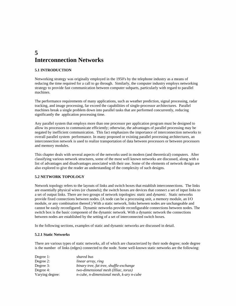
N, where a0, a1, ... aN are the coefficients and x is a variable. As an example, consider the evaluation of a polynomial of degree 7. One way to evaluate such a polynomial is to use the architecture given in Figure 5.7. In this figure, assume that each node represents a processor having three registers: one to hold the coefficient, one to hold the variable x, and the third to hold a bit called the mask bit. Figure 5.8 illustrates the three registers of a node.

Figure 5.8 A shuffle-exchange node's registers.

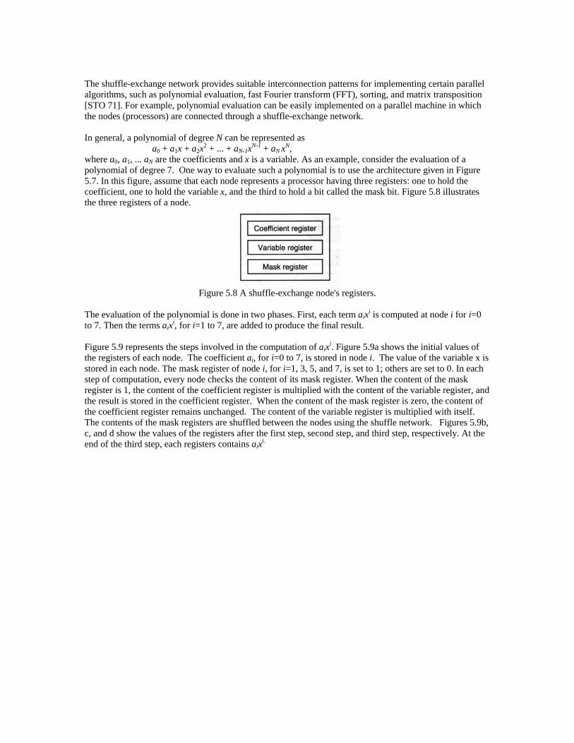
The evaluation of the polynomial is done in two phases. First, each term aix

i is computed at node i for i=0 to 7. Then the terms aix

i, for i=1 to 7, are added to produce the final result. Figure 5.9 represents the steps involved in the computation of aix

i. Figure 5.9a shows the initial values of the registers of each node. The coefficient ai, for i=0 to 7, is stored in node i. The value of the variable x is stored in each node. The mask register of node i, for i=1, 3, 5, and 7, is set to 1; others are set to 0. In each step of computation, every node checks the content of its mask register. When the content of the mask register is 1, the content of the coefficient register is multiplied with the content of the variable register, and the result is stored in the coefficient register. When the content of the mask register is zero, the content of the coefficient register remains unchanged. The content of the variable register is multiplied with itself. The contents of the mask registers are shuffled between the nodes using the shuffle network. Figures 5.9b, c, and d show the values of the registers after the first step, second step, and third step, respectively. At the end of the third step, each registers contains aix

i.

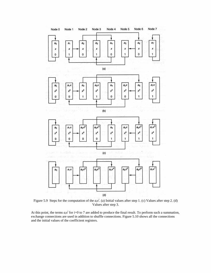
Figure 5.9 Steps for the computation of the aix

i. (a) Initial values after step 1. (c) Values after step 2. (d) Values after step 3.

At this point, the terms aix

i for i=0 to 7 are added to produce the final result. To perform such a summation, exchange connections are used in addition to shuffle connections. Figure 5.10 shows all the connections and the initial values of the coefficient registers.

Figure 5.10 Required connections for adding the terms aix

i. In each step of computation the contents of the coefficient registers are shuffled between the nodes using the shuffle connections. Then copies of the contents of the coefficient registers are exchanged between the nodes using the exchange connections. After the exchange is performed, each node adds the content of its coefficient register to the value that the copy of the current content is exchanged with. After three shuffle

and exchanges, the content of each coefficient register will be the desired

7

0ixi

ai . The following shows

the three steps required to obtain result .

As you can see in the chart, after the third step, the value

7

0ixi

ai is stored in each coefficient register.

From this example, it should be apparent that the shuffle-exchange network provides the desired connections for manipulating the values of certain problems efficiently. Two-dimensional mesh. A two-dimensional mesh consists of k1*k0 nodes, where ki 2 denotes the number of nodes along dimension i. Figure 5.11 represents a two-dimensional mesh for k0=4 and k1=2. There are four nodes along dimension 0, and two nodes along dimension 1. As shown in Figure 5.11, in a two-dimensional mesh network each node is connected to its north, south, east, and west neighbors. In general, a node at row i and column j is connected to the nodes at locations (i-1, j), (i+1, j), (i, j-1), and (i, j+1). The nodes on the edge of the network have only two or three immediate neighbors. The diameter of a mesh network is equal to the distance between nodes at opposite corners. Thus, a two-dimensional mesh with k1*k0 nodes has a diameter (k1 -1) + (k0-1).

Figure 5.11 A two-dimensional mesh with k0=4 and k1=2.

In practice, two-dimensional meshes with an equal number of nodes along each dimension are often used for connecting a set of processing nodes. For this reason in most literature the notion of two-dimensional mesh is used without indicating the values for k1 and k0; rather, the total number of nodes is defined. A two-dimensional mesh with k1=k0=n is usually referred to as a mesh with N nodes, where N = n2. For example, Figure 5.12 shows a mesh with 16 nodes. From this point forward, the term mesh will indicated a two-dimensional mesh with an equal number of nodes along each dimension.

Figure 5.12 A two-dimensional mesh with k0=k1=4.

The routing of data through a mesh can be accomplished in a straightforward manner. The following simple routing algorithm routes a packet from source S to destination D in a mesh with n2 nodes.

1. Compute the row distance R as nSnDR // .

2. Compute the column distance C as )(mod)(mod nSnDC .

3. Add the values R and C to the packet header at the source node. 4. Starting from the source, send the packet for R rows and then for C columns.

The values R and C determine the number of rows and columns that the packet needs to travel. The direction the message takes at each node is determined by the sign of the values R and C. When R (C) is positive, the packet travels downward (right); otherwise, the packet travels upward (left). Each time that the packet travels from one node to the adjacent node downward, the value R is decremented by 1, and when it travels upward, R is incremented by 1. Once R becomes 0, the packet starts traveling in the horizontal

direction. Each time that the packet travels from one node to the adjacent node in the right direction, the value C is decremented by 1, and when it travels in the left direction, C is incremented by 1. When C becomes 0, the packet has arrived at the destination. For example, to route a packet from node 6 (i.e., S=6) to node 12 (i.e., D= 12), the packet goes through two paths, as shown in Figure 5.13. In this example,

,24/64/12 R

220 C

Figure 5.13 Routing path from node 6 to node 12.

It should be noted that in the case just described the nodes on the edge of the mesh network have no connections to their far neighbors. When there are such connections, the network is called a wraparound two-dimensional mesh, or an Illiac network. An Illiac network is illustrated in Figure 5.14 for N = 16.

Figure 5.14 A 16-node Illiac network.

In general, the connections of an Illiac network can be defined by the following four functions: Illiac+1(j) = j+1 (mod N), Illiac-1(j) = j-1 (mod N), Illiac+n(j) = j+n (mod N), Illiac-n(j) = j-n (mod N), where N is the number of nodes, 0 j < N, n is the number of nodes along any dimension, and N=n2. For example, in Figure 5.14, node 4 is connected to nodes 5, 3, 8, and 0, since Illiac+1 (4) = ( 4 + 1 ) (mod 16) = 5, Illiac-1 (4) = ( 4 - 1 ) (mod 16) = 3, Illiac+4 (4) = ( 4 + 4 ) (mod 16) = 8, Illiac-4 (4) = ( 4 - 4 ) (mod 16) = 0. The diameter of an Illiac with N=n2 nodes is n-1, which is shorter than a mesh. Although the extra wraparound connections in Illiac allow the diameter to decrease, they increase the complexity of the design.

Figure 5.15 shows the connectivity of the nodes in a different form. This graph shows that four nodes can be reached from any node in one step, seven nodes in two steps, and four nodes in three steps. In general, the number of steps (recirculations) to route data from a node to any other node is upper bounded by the diameter (i.e., n – 1).

Figure 5.15 Alternative representation of a 16-node Illiac network.

To reduce the diameter of a mesh network, another variation of this network, called torus (or two-dimensional tours), has also been proposed. As shown in Figure 5.16a, a torus is a combination of ring and mesh networks. To make the wire length between the adjacent nodes equal, the torus may be folded as shown in Figure 5.16b. In this way the communication delay between the adjacent nodes becomes equal. Note that both Figures 5.16a and b provide the same connections between the nodes; in fact, Figure 5.16b is derived from Figure 5.16a by switching the position of the rightmost two columns and the bottom two rows of nodes. The diameter of a torus with N=n2 nodes is 2/2 n , which is the distance between the corner

and the center node. Note that the diameter is further decreased from the mesh network.

Figure 5.16 Different types of torus network. (a) A 4-by-4 torus network. (b) A 4-by-4 torus network with

folded connection.

The mesh network provides suitable interconnection patterns for problems whose solutions require the computation of a set of values on a grid of points, for which the value at each point is determined based on the values of the neighboring points. Here we consider one of these class of problems: the problem of finding a steady-state temperature over the surface of a square slab of material whose four edges are held at different temperatures. This problem requires the solution of the following partial differential equation, known as Laplace's equation:

0// 2222 yUxU ,

where U is the temperature at a given point specified by the coordinates x and y on the slab. The following describes a method, given by Slotnick [SLO 71], to solve this problem. Even if unfamiliar with Laplace's equation, the reader should still be able to follow the description. The method is based on the fact that the temperature at any point on the slab tends to become the average of the temperatures of neighboring points. Assume that the slab is covered with a mesh and that each square of the mesh has h units on each side. Then the temperature of an interior node at coordinates x and y is the average of the temperatures of the four neighbor nodes. That is, the temperature at node (x, y), denoted as U(x, y), equals the sum of the four neighboring temperatures divided by 4. For example, as shown in Figure 5.17, assume that the slab can be covered with a 16-node mesh. Here the value of U(x, y) is expressed as

U(x,y)=[U(x,y+h) + U(x+h,y) + U(x,y-h) + U(x-h,y)]/4.

Figure 5.17 Covering a slab with a 16-node mesh.

Figure 5.18 illustrates an alternative representation of Figure 5.17. Here the position of the nodes is more conveniently indicated by the integers i and j. In this case, the temperature equation can be expressed as

U(i,j)=[U(i,j+1) + U(i+1,j) + U(i,j-1) + U(i-1,j)]/4. Assume that each node represents a processor having one register to hold the node's temperature. The nodes on the boundary are arbitrarily held at certain fixed temperatures. Let the nodes on the bottom of the mesh and on the right edge be held at zero degrees. The nodes along the top and left edges are set according to their positions. The temperatures of these 12 boundary nodes do not change during the computation. The temperatures at the 4 interior nodes are the unknowns. Initially, the temperatures at these 4 nodes are set to zero. In the first iteration of computation, the 4 interior node processors simultaneously calculate the new temperature values using the values initially given.

Figure 5.18 Initial values of the nodes.

Figure 5.19 represents the new values of the interior nodes after the first iteration. These values are calculated as follows: U(1,2)=[U(1,3)+U(2,2)+U(1,1)+U(0,2)]/4 = [8+0+0+8]/4 = 4; U(2,2)=[U(2,3)+U(3,2)+U(2,1)+U(1,2)]/4 = [4+0+0+0]/4 = 1; U(1,1)=[U(1,2)+U(2,1)+U(1,0)+U(0,1)]/4 = [0+0+0+4]/4 = 1; U(2,1)=[U(2,2)+U(3,1)+U(2,0)+U(1,1)]/4 = [0+0+0+0]/4 = 0. In the second iteration, the values of U(1,2), U(2,2), U(1,1), and U(2,1) are calculated using the new values just obtained: U(1,2) = [8+1+1+8]/4 = 4.5; U(2,2) = [4+0+0+4]/4 = 2; U(1,1) = [4+0+0+4]/4 = 2; U(2,1) = [1+0+0+1]/4 = 0.5. This process continues until a steady-state solution is obtained. As more iterations are performed, the values of the interior nodes converge to the exact solution. When values for two successive iterations are close to each other (within a specified error tolerance), the process can be stopped, and it can be said that a steady-state solution has been reached. Figure 5.20 represents a solution obtained after 11 iterations.

Figure 5.19 Values of the nodes after the first iteration.

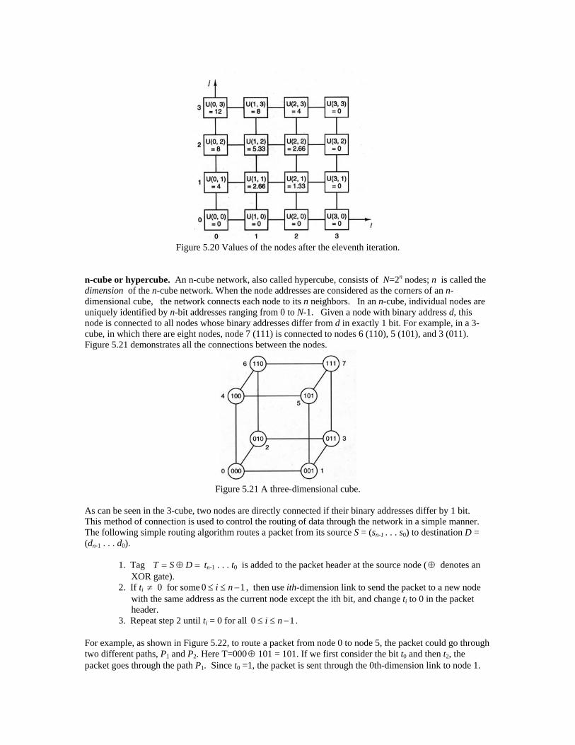
Figure 5.20 Values of the nodes after the eleventh iteration.

n-cube or hypercube. An n-cube network, also called hypercube, consists of N=2n nodes; n is called the dimension of the n-cube network. When the node addresses are considered as the corners of an n-dimensional cube, the network connects each node to its n neighbors. In an n-cube, individual nodes are uniquely identified by n-bit addresses ranging from 0 to N-1. Given a node with binary address d, this node is connected to all nodes whose binary addresses differ from d in exactly 1 bit. For example, in a 3-cube, in which there are eight nodes, node 7 (111) is connected to nodes 6 (110), 5 (101), and 3 (011). Figure 5.21 demonstrates all the connections between the nodes.

Figure 5.21 A three-dimensional cube.

As can be seen in the 3-cube, two nodes are directly connected if their binary addresses differ by 1 bit. This method of connection is used to control the routing of data through the network in a simple manner. The following simple routing algorithm routes a packet from its source S = (sn-1 . . . s0) to destination D = (dn-1 . . . d0).

1. Tag DST tn-1 . . . t0 is added to the packet header at the source node ( denotes an XOR gate).

2. If ti 0 for some 10 ni , then use ith-dimension link to send the packet to a new node with the same address as the current node except the ith bit, and change ti to 0 in the packet header.

3. Repeat step 2 until ti = 0 for all 10 ni . For example, as shown in Figure 5.22, to route a packet from node 0 to node 5, the packet could go through two different paths, P1 and P2. Here T=000 101 = 101. If we first consider the bit t0 and then t2, the packet goes through the path P1. Since t0 =1, the packet is sent through the 0th-dimension link to node 1.

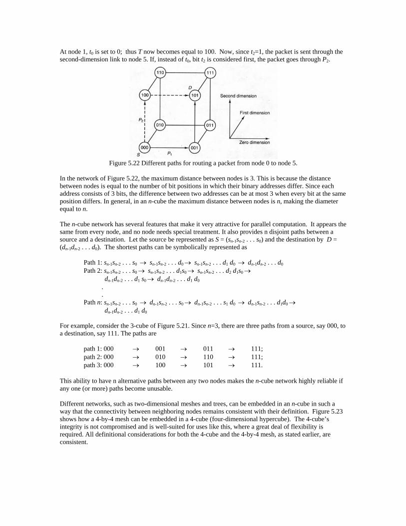
At node 1, t0 is set to 0; thus T now becomes equal to 100. Now, since t2=1, the packet is sent through the second-dimension link to node 5. If, instead of t0, bit t2 is considered first, the packet goes through P2.

Figure 5.22 Different paths for routing a packet from node 0 to node 5.

In the network of Figure 5.22, the maximum distance between nodes is 3. This is because the distance between nodes is equal to the number of bit positions in which their binary addresses differ. Since each address consists of 3 bits, the difference between two addresses can be at most 3 when every bit at the same position differs. In general, in an n-cube the maximum distance between nodes is n, making the diameter equal to n. The n-cube network has several features that make it very attractive for parallel computation. It appears the same from every node, and no node needs special treatment. It also provides n disjoint paths between a source and a destination. Let the source be represented as S = (sn-1sn-2 . . . s0) and the destination by D = (dn-1dn-2 . . . d0). The shortest paths can be symbolically represented as

Path 1: sn-1sn-2 . . . s0 sn-1sn-2 . . . d0 sn-1sn-2 . . . d1 d0 dn-1dn-2 . . . d0 Path 2: sn-1sn-2 . . . s0 sn-1sn-2 . . . d1s0 sn-1sn-2 . . . d2 d1s0

dn-1dn-2 . . . d1 s0 dn-1dn-2 . . . d1 d0 . .

Path n: sn-1sn-2 . . . s0 dn-1sn-2 . . . s0 dn-1sn-2 . . . s1 d0 dn-1sn-2 . . . d1d0 dn-1dn-2 . . . d1 d0

For example, consider the 3-cube of Figure 5.21. Since n=3, there are three paths from a source, say 000, to a destination, say 111. The paths are

path 1: 000 001 011 111; path 2: 000 010 110 111; path 3: 000 100 101 111.

This ability to have n alternative paths between any two nodes makes the n-cube network highly reliable if any one (or more) paths become unusable. Different networks, such as two-dimensional meshes and trees, can be embedded in an n-cube in such a way that the connectivity between neighboring nodes remains consistent with their definition. Figure 5.23 shows how a 4-by-4 mesh can be embedded in a 4-cube (four-dimensional hypercube). The 4-cube’s integrity is not compromised and is well-suited for uses like this, where a great deal of flexibility is required. All definitional considerations for both the 4-cube and the 4-by-4 mesh, as stated earlier, are consistent.

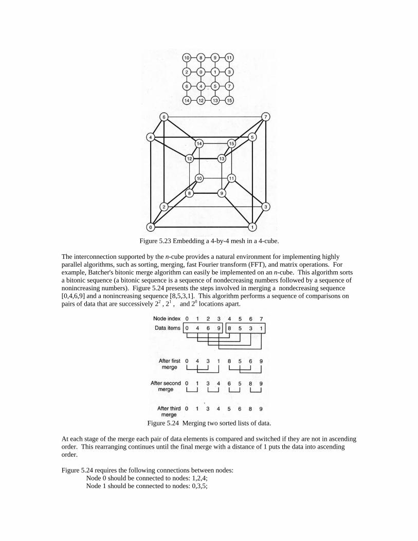
Figure 5.23 Embedding a 4-by-4 mesh in a 4-cube.

The interconnection supported by the n-cube provides a natural environment for implementing highly parallel algorithms, such as sorting, merging, fast Fourier transform (FFT), and matrix operations. For example, Batcher's bitonic merge algorithm can easily be implemented on an n-cube. This algorithm sorts a bitonic sequence (a bitonic sequence is a sequence of nondecreasing numbers followed by a sequence of nonincreasing numbers). Figure 5.24 presents the steps involved in merging a nondecreasing sequence [0,4,6,9] and a nonincreasing sequence [8,5,3,1]. This algorithm performs a sequence of comparisons on pairs of data that are successively 22 , 21 , and 20 locations apart.

Figure 5.24 Merging two sorted lists of data.

At each stage of the merge each pair of data elements is compared and switched if they are not in ascending order. This rearranging continues until the final merge with a distance of 1 puts the data into ascending order. Figure 5.24 requires the following connections between nodes: Node 0 should be connected to nodes: 1,2,4; Node 1 should be connected to nodes: 0,3,5;

Node 2 should be connected to nodes: 0,3,6; Node 3 should be connected to nodes: 1,2,7; Node 4 should be connected to nodes: 0,5,6; Node 5 should be connected to nodes: 1,4,7; Node 6 should be connected to nodes: 2,4,7; Node 7 should be connected to nodes: 3,5,6. These are exactly the same as 3-cube connections. That is, the n-cube provides the necessary connections for the Batcher's algorithm. Thus, applying Batcher's algorithm to an n-cube network is straightforward. In general, the n-cube provides the necessary connections for ascending and descending classes of parallel algorithms. To define each of these classes, assume that there are 2n input data items stored in 2n locations (or processors) 0, 1, 2, ..., 2n -1. An algorithm is said to be in the descending class if it performs a sequence of basic operations on pairs of data that are successively 2n-1 , 2n-2 , ..., and 20 locations apart. (Therefore, Batcher's algorithm belongs to this class.) In comparison, an ascending algorithm performs successively on pairs that are 20, 21, ..., and 2n-1 locations apart. When n=3 Figures 5.25 and 5.26 show the required connections for each stage of operation in this class of algorithms. As shown, the n-cube is able to efficiently implement algorithms in descending or ascending classes.

Figure 5.25 Descending class.

Figure 5.26 Ascending class.

Although the n-cube can implement this class of algorithms in n parallel steps, it requires n connections for each node, which makes the design and expansion difficult. In other words, the n-cube provides poor scalability and has an inefficient structure for packaging and therefore does not facilitate the increasingly important property of modular design. n-Dimensional mesh. An n-dimensional mesh consists of kn-1*kn-2*....*k0 nodes, where ki 2 denotes the number of nodes along dimension i. Each node X is identified by n coordinates xn-1,xn-2, ... , x0, where 0 xi ki -1 for 0 i n-1. Two nodes X=(xn-1,xn-2,...,x0) and Y=(yn-1,yn-2,...,y0) are said to be neighbors if and only if yi=xi for all i, 0 i n-1, except one, j, where yj=xj + 1 or yj=xj - 1. That is, a node may have from n to 2n neighbors, depending on its location in the mesh. The corners of the mesh have n neighbors, and the internal nodes have 2n neighbors, while other nodes have nb neighbors, where n<nb<2n. The diameter of

an n-dimensional mesh is

1

0)1(

n

iik . An n-cube is a special case of n-dimensional meshes; it is in fact an n-

dimensional mesh in which ki=2 for 0 i n-1. Figure 5.27 represents the structure of two three-

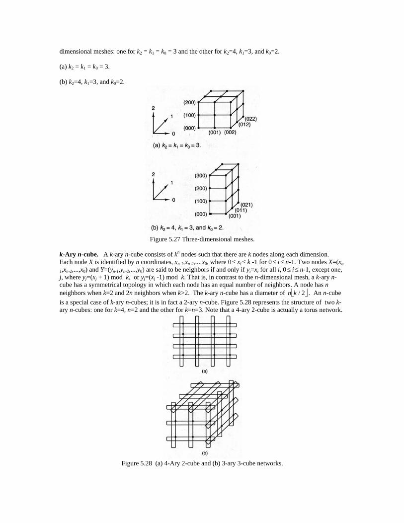
dimensional meshes: one for k2 = k1 = k0 = 3 and the other for k2=4, k1=3, and k0=2. (a) k2 = k1 = k0 = 3. (b) k2=4, k1=3, and k0=2.

Figure 5.27 Three-dimensional meshes.

k-Ary n-cube. A k-ary n-cube consists of kn nodes such that there are k nodes along each dimension. Each node X is identified by n coordinates, xn-1,xn-2,...,x0, where 0 xi k -1 for 0 i n-1. Two nodes X=(xn-

1,xn-2,...,x0) and Y=(yn-1,yn-2,...,y0) are said to be neighbors if and only if yi=xi for all i, 0 i n-1, except one, j, where yj=(xj + 1) mod k, or yj=(xj -1) mod k. That is, in contrast to the n-dimensional mesh, a k-ary n-cube has a symmetrical topology in which each node has an equal number of neighbors. A node has n neighbors when k=2 and 2n neighbors when k>2. The k-ary n-cube has a diameter of 2/kn . An n-cube

is a special case of k-ary n-cubes; it is in fact a 2-ary n-cube. Figure 5.28 represents the structure of two k-ary n-cubes: one for k=4, n=2 and the other for k=n=3. Note that a 4-ary 2-cube is actually a torus network.

Figure 5.28 (a) 4-Ary 2-cube and (b) 3-ary 3-cube networks.

Routing in n-dimensional meshes and k-ary n-cubes. One of the routing algorithms that can be used for routing the packets within an n-dimensional mesh or a k-ary n-cube is called store-and-forward routing [TAN 81]. Each node of the network contains a buffer equal to the size of a packet. In store-and-forward routing, a packet is transmitted from a source node to a destination node through a sequence of intermediate nodes. Each intermediate node of the network receives a packet in its entirety before transmitting it to the next node. When an intermediate node receives a packet, it first stores the packet in its buffer; then it forwards the packet to the next node when the receiving node's buffer is empty. Store-and-forward routing is easy to understand and simple to implement. However, it requires a transmission time proportional to the distance (the number of hops or channels) between the source and the destination nodes to deliver a packet. (Channels are actually electrical connections between nodes and are arranged based on the network topology.) To reduce transmission time and make this task almost independent of the distance between source and destination nodes, a hardware-supported routing protocol, called wormhole routing (also direct-connect routing ) is often used. In wormhole routing, a packet is divided into several smaller data units, called flits. Only the first flit (the leading flit) carries the routing information (such as the destination address), and the remaining flits follow this leader. Once a leader flit arrives at a node, the node selects the outgoing channel based on the flit's routing information and begins forwarding the flits through that channel. Since the remaining flits carry no routing information, they must necessarily follow the channels established by the header for the transmission to be successful. Therefore, they cannot be interleaved (alternated or mixed) with the flits of other packets. When a leader flit arrives at a node that has no output channel available, all the flits remain in their current position until a suitable channel becomes available. Each node contains a few small buffers for storing such flits. At each node, the selection of an outgoing channel for a particular leading flit depends on the incoming channel (the channel that was used by the flit to enter the node) and the destination node. This type of dependency can be represented by a channel dependency graph. A channel dependency graph for a given interconnection network together with a routing algorithm is a directed graph such as shown in Figure 5.29b. The vertices of the graph in Figure 5.29b are the channels of the network, and the edges are the pairs of channels connected by the routing algorithm. For example, consider Figure 5.29a, where a network with nodes n11, n10, ..., and n00 and unidirectional channels c11, c10, ..., and c00, is shown. The channels are labeled by the identification number (id) of their source node. A routing algorithm for such a network could advance the flits on c11 to c10, on c10 to c01, and so on. Based on this routing algorithm, Figure 5.29b represents the dependency graph for such a network. Notice that the dependency graph consists of a cycle that may cause a deadlock in the network. A deadlock can occur whenever no flits can proceed toward their destinations because the buffers on the route are full. Figure 5.29c presents a deadlock configuration in the case when there are two buffers in each node.

Figure 5.29 A simple network with four nodes. (a) Network. (b) Dependency graph. (c) Deadlock.

To have reliable and efficient communication between nodes, a deadlock-free routing algorithm is needed. Dally and Seitz [DAL 87] have shown that a routing algorithm for an interconnection network is deadlock free if and only if there are no cycles (a route that reconnects with itself) in the channel dependency graph. Their proposal is to avoid deadlock by eliminating cycles through the use of virtual channels. A virtual channel is a logical link between two nodes formed by a physical channel and a flit buffer in each of the two nodes. Each physical channel is shared among a group of virtual channels. Although several virtual channels share a physical channel, each virtual channel has its own buffer. With many (virtual) channels to choose from, cycles, and therefore deadlock, can be avoided.

Figure 5.30a represents the virtual channels for a network when each physical channel is split into two virtual channels: lower virtual channels and upper virtual channels. The lower virtual channel of cx (where x is identified as the source node) is labeled c0x, and the upper virtual channel is labeled c1x. For example, the lower virtual channel of c11 is numbered as c011. Dally and Seitz's routing algorithm routes packets at a node with a label value less than the destination node on the upper virtual channels and routes packets at a node labeled greater than their destination node on the lower channels. This routing algorithm restricts the packets' routing to the order of decreasing virtual channel labels. Thus there is no cycle in the dependency graph and the network is deadlock free (see Figure 5.30b).

Figure 5.30 (a) Virtual channels and (b) dependency graph for a simple network with four nodes.

Wormhole routing is based on a method of dividing packets into smaller transmission units called flits. Transmitting flits rather than packets reduces the average time required to deliver a packet in the network, as shown in Figure 5.31.

Figure 5.31 Comparing (a) store-and-forward routing with (b) wormhole routing. Tsf and Twh are average transmission time over three channels when using store-and-forward routing and wormhole routing, respectively. For example, assume that each packet consists of q flits, and Tf is the amount of time required for each flit to be transmitted across a single channel. The amount of time required to transmit a packet over a single channel is therefore q*Tf. With store-and-forward routing, the average time required to transmit a packet over D channels will be D*q*Tf. However, with wormhole routing, in which the flits are forwarded in a

pipeline fashion, the average transmission time over D channels becomes (q+D-1)*Tf. This means that wormhole routing is much faster than store-and-forward routing. Furthermore, wormhole routing requires very little storage, resulting in a small and fast communication controller. In general, it is an efficient routing technique for k-ary n-cubes and n-dimensional meshes. In literature, several deadlock-free routing algorithms, based on the wormhole routing concept, have been proposed. These algorithms can be classified into two groups: deterministic (or static) routing and adaptive (or dynamic) routing. In deterministic routing, the routing path, which is traversed by flits, is fixed and is determined by the source and destination addresses. Although, these routings usually select one of the shortest paths between the source and destination nodes, they limit the ability of the interconnection network to adapt itself to failures or heavy traffic (congestion) along the intended routes. It is in this case that adaptive routing becomes important. Adaptive routing algorithms allow the path taken by flits to depend on dynamic network conditions (such as the presence of faulty or congested channels), rather than source and destination addresses. The description of these algorithms is beyond the scope of this book. The reader can refer to [NI 93] for a survey on deterministic and adaptive wormhole routing in k-ary n-cubes and n-dimensional meshes. Network Latency. Here, based on the work of Agarwal [AGA 91] and Dally and Seitz[DAL 87], we focus on deriving an equation for the average time required to transmit a packet in k-ary n-cubes that uses wormhole routing. A similar analysis can also be carried out for n-dimentional networks. We assume that the networks are embedded in a plane and have unidirectional channels. The network latency, Tb, refers to the elapsed time from the time that the first flit of the packet leaves the source to the time the last flit arrives at the destination. Hence, ignoring the network load, Tb can be expressed as Tb = (q+D-1)*Tf, where D denotes the number of channels (hops) that a packet traverses. Let Tf be represented as the sum of the wire delay Tw(n) and node delay Ts, that is, Tf = Tw(n) + Ts. Hence, Tb = (q+D-1)[ Tw(n) + Ts]. The number of channels, D, can be determined by the product of the network dimension and the average distance (kd) that a packet must travel in each dimension of the network. Assuming that the packet destinations are randomly chosen, the average distance a packet must travel is given by kd =(k-1)/2. Hence Tb = [q + n(k-1)/2 -1][ Tw(n) + Ts]. To determine Tw(n), we must find the length of the longest wire of an n-dimensional network embedded in a plane. The embedding of an n-dimensional network in a plane can be achieved by mapping n/2 dimensions of the network in each of the two physical dimensions. That is, the number of nodes in each physical dimension is kn/2. Thus each additional dimension of the network increases the number of nodes in each physical dimension by k1/2. Assuming that the distance between the physically adjacent nodes remains fixed, each additional dimension also increases the length of the longest wire length by a factor of k1/2. Assume that the wire delay depends linearly on the wire length. If we consider the delay of a wire in a two-dimensional network [i.e., Tw(2)] as a base time period, the delay of the longest wire is given by Tw(n) = (k1/2)n-2 Tw(2) = k(n/2 - 1). Hence

Tb = [q + n(k-1)/2 -1][ k(n/2 - 1) +Ts]. Agarwal [AGA 91] has extended this result to the analysis of a k-ary n-cube under different load parameters, such as packet size, degree of local communication, and network request rate. [The degree of local communication increases as the probability of communication with (or access to) various nodes decreases as a function of physical distance.] Agarwal has shown that two-dimensional networks have the lowest latency when node delays and network contention are ignored. Otherwise, three or four dimensions are preferred. However, when the degree of local communications becomes high, two-dimensional networks outperform three- and four-dimensional networks. Local communication depends on several factors, such as machine architecture, type of applications, and compiler. If these factors are enhanced, two-dimensional networks can be used without incurring the high cost of higher dimensions. Another alternative for enhancing local communication is to provide short paths for nonlocal packets. The k-ary n-cube network can be augmented by one or more levels of express channels that allow nonlocal messages to bypass nodes [DAL 91]. The augmented network, called express cube, reduces the network diameter and increases the wire length. This arrangement allows the network to operate with latencies that approach the physical speed-of-light limitation, rather than being limited by node delays. Figure 5.32 illustrates the addition of express channels to a k-ary 1-cube network. In express cubes the wire length of express channels can be increased to the point that wire delays dominate node delay, making low-dimensional networks more attractive.

Figure 5.32 Express cube. (a) Regular k-ary 1-cube network. (b) k-ary 1-cube network with express

channels. 5.2.2 Dynamic Networks Dynamic networks provide reconfigurable connections between nodes. The topology of a dynamic network is the physical structure of the network as determined by the switch boxes and the interconnecting links. Since the switch box is the basic component of the network, the cost of the network (in hardware terms) is measured by the number of switch boxes required. Therefore, the topology of the network is the prime determinant of the cost. To clarify the preceding terminology, let us consider the design of a dynamic network using simple switch boxes. Figure 5.33 represents a simple switch with two inputs (x and y) and two outputs (z0 and z1). A control line, s, determines whether the input lines should be connected to the output lines in straight state or exchange state. For example, when the control line s=0, the inputs are connected to the outputs in a straight state; that is, x is connected to z0 and y is connected to z1. When the control line s=1, the inputs are connected to outputs in an exchange state; that is, x is connected to z1 and y is connected to z0.

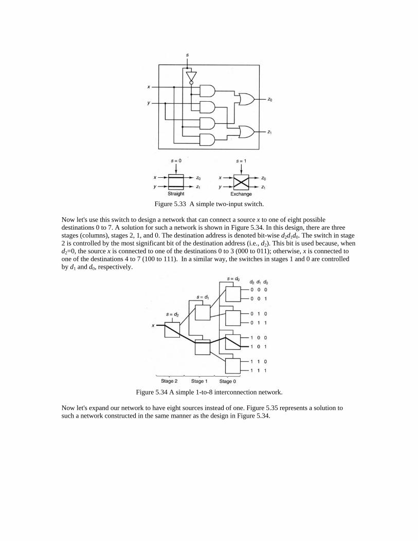
Figure 5.33 A simple two-input switch.

Now let's use this switch to design a network that can connect a source x to one of eight possible destinations 0 to 7. A solution for such a network is shown in Figure 5.34. In this design, there are three stages (columns), stages 2, 1, and 0. The destination address is denoted bit-wise d2d1d0. The switch in stage 2 is controlled by the most significant bit of the destination address (i.e., d2). This bit is used because, when d2=0, the source x is connected to one of the destinations 0 to 3 (000 to 011); otherwise, x is connected to one of the destinations 4 to 7 (100 to 111). In a similar way, the switches in stages 1 and 0 are controlled by d1 and d0, respectively.

Figure 5.34 A simple 1-to-8 interconnection network.

Now let's expand our network to have eight sources instead of one. Figure 5.35 represents a solution to such a network constructed in the same manner as the design in Figure 5.34.

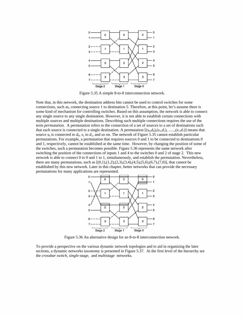
Figure 5.35 A simple 8-to-8 interconnection network.

Note that, in this network, the destination address bits cannot be used to control switches for some connections, such as, connecting source 1 to destination 5. Therefore, at this point, let’s assume there is some kind of mechanism for controlling switches. Based on this assumption, the network is able to connect any single source to any single destination. However, it is not able to establish certain connections with multiple sources and multiple destinations. Describing such multiple connections requires the use of the term permutation. A permutation refers to the connection of a set of sources to a set of destinations such that each source is connected to a single destination. A permutation [(s0,d0),(s1,d1), ......,(s7,d7)] means that source s0 is connected to d0, s1 to d1, and so on. The network of Figure 5.35 cannot establish particular permutations. For example, a permutation that requires sources 0 and 1 to be connected to destinations 0 and 1, respectively, cannot be established at the same time. However, by changing the position of some of the switches, such a permutation becomes possible. Figure 5.36 represents the same network after switching the position of the connections of inputs 1 and 4 to the switches 0 and 2 of stage 2. This new network is able to connect 0 to 0 and 1 to 1, simultaneously, and establish the permutation. Nevertheless, there are many permutations, such as [(0,1),(1,2),(2,3),(3,4),(4,5),(5,6),(6,7),(7,0)], that cannot be established by this new network. Later in this chapter, better networks that can provide the necessary permutations for many applications are represented.

Figure 5.36 An alternative design for an 8-to-8 interconnection network.

To provide a perspective on the various dynamic network topologies and to aid in organizing the later sections, a dynamic networks taxonomy is presented in Figure 5.37. At the first level of the hierarchy are the crossbar switch, single-stage, and multistage networks.

Figure 5.37 Classification of dynamic networks.

The crossbar switch can be used for connecting a set of input nodes to a set of output nodes. In this network every input node can be connected to any output node. The crossbar switch provides all possible permutations, as well as support for high system performance. It can be viewed as a number of vertical and horizontal links interconnected by a switch at each intersection. Figure 5.38 represents a crossbar for connecting N nodes to N nodes. The connection between each pair of nodes is established by a crosspoint switch. The crosspoint switch can be set on or off in response to application needs. There are N2 crosspoint switches for providing complete connections between all the nodes. The crossbar switch is an ideal network to use for small N. However, for large N, the implementation of the crosspoint switches makes this design complex and expensive and thus less attractive to use.

Figure 5.38 Crossbar switch.

Single-stage networks, also called recirculating networks, require routing algorithms to direct the flow of data several times through the network so that various connections and permutations can be constructed. Each time that the data traverse the network is called a pass. As an example, Figure 5.39 represents a single-stage network based on the shuffle-exchange connection. Multistage networks, such as the one in Figure 5.36, are more complex from a hardware point of view, but the routing of data is made simpler by virtue of permanent connections between the stages of the network. Because there are more switches in a multistage network, the number of possible permutations on a single pass increases; however, there is a higher investment in hardware. There is also a possible reduction in the complexity of routing functions and the time it takes to generate the necessary permutations.

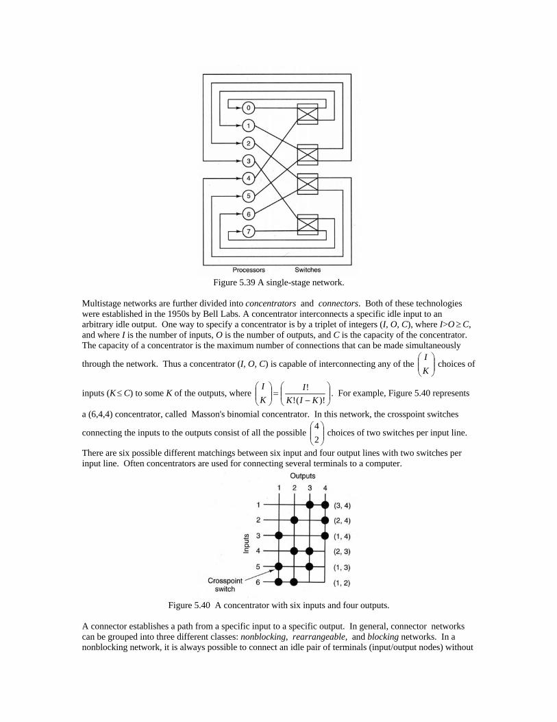
Figure 5.39 A single-stage network.

Multistage networks are further divided into concentrators and connectors. Both of these technologies were established in the 1950s by Bell Labs. A concentrator interconnects a specific idle input to an arbitrary idle output. One way to specify a concentrator is by a triplet of integers (I, O, C), where I>OC, and where I is the number of inputs, O is the number of outputs, and C is the capacity of the concentrator. The capacity of a concentrator is the maximum number of connections that can be made simultaneously

through the network. Thus a concentrator (I, O, C) is capable of interconnecting any of the

K

I choices of

inputs (KC) to some K of the outputs, where

)!(!

!

KIK

I

K

I. For example, Figure 5.40 represents

a (6,4,4) concentrator, called Masson's binomial concentrator. In this network, the crosspoint switches

connecting the inputs to the outputs consist of all the possible

2

4 choices of two switches per input line.

There are six possible different matchings between six input and four output lines with two switches per input line. Often concentrators are used for connecting several terminals to a computer.

Figure 5.40 A concentrator with six inputs and four outputs.

A connector establishes a path from a specific input to a specific output. In general, connector networks can be grouped into three different classes: nonblocking, rearrangeable, and blocking networks. In a nonblocking network, it is always possible to connect an idle pair of terminals (input/output nodes) without

disturbing connections (calls) already in progress. This is called "nonblocking in the strict sense" simply because such a network has no blocking states whatsoever. These type of networks are said to be universal networks since they can provide all possible permutations. The rearrangeable networks are also universal networks; however, in this type of network it may not always be possible to connect an idle pair of terminals without disturbing established connections. In a rearrangeable network, given any set of connections in progress and any pair of idle terminals, the existing connections can be reassigned new routes (if necessary) so as to make it possible to connect the idle pair at any time. In contrast, in a blocking network, depending on what state the network may be in, it may not be possible to connect an idle pair of terminals in any way. For each group of connectors, a class of dynamic networks is shown in the following discussion. Nonblocking networks. Clos has proposed a class of networks with interesting properties [CLO 53]. Figure 5.41 shows one example of such a network. This particular network is called a three-stage Clos network. It consists of an input stage of mn crossbar switches, an output stage of nm crossbar switches, and a middle stage of rr crossbar switches. This class of networks is denoted by the triple N(m,n,r), which determines the switches' dimensions.

Figure 5.41 A nonblocking network

Clos has shown that for m 2n-1, the network N(m,n,r), is a nonblocking network. For example, the network N(3,2,2) in Figure 5.42 is a nonblocking network. This network requires 12 crosspoint switches in every stage, or 36 switches in all. Note that a crossbar switch with the same number of inputs and outputs (i.e., 4) requires 16 switches. Thus in this case it is more economical to design a crossbar switch than a Clos network. However, when the number of inputs, N, increases, the number of switches becomes much less than N2, as in the case of the crossbar. For example, for N=36, only 1188 switches are necessary in a Clos network, whereas in the case of a crossbar network 362, or 1296, switches are required.

Figure 5.42 A Clos network with n=2, r=2, and m=3.

There should be at least 2n-1 switches in the middle stage of the Clos network in order to become a nonblocking network. To demonstrate the necessity of this condition, let's consider the following example. Figure 5.43 represents a section of a Clos network in which each input (output) switch has three inputs

(outputs). Let's assume that we want to connect input C to output F. In this example, four middle switches are required to permit inputs other than C (i.e., A and B) on a particular input switch and outputs other than F (i.e., D and E) on a particular output switch to have connections to separate middle switches. In addition, one more switch for the desired connection between C and F is required. Thus five middle switches are required (i.e., 2*3-1 switches). A similar argument can be given for a general network N(m,n,r), in order to show that N is nonblocking when m=2n-1.

Figure 5.43 A portion of a Clos network in which each input/output switch has three terminals.

The total number of switches for a three-stage Clos network N(2n-1, n, n) can be obtained by analyzing the number of switches in each stage. Assuming that the network has N input terminals, where N=n2, then The input stage contains n2(2n-1) switches. The middle stage contains n2(2n-1) switches. The output stage contains n2(2n-1) switches. Therefore, the total number of switches, C(3), is C(3) = (2n-1)(3n2)=6n3-3n2. In a similar way, the total number of switches for a five-stage Clos network, shown in Figure 5.44, is C(5) = (2n-1)(6n3-3n2)+2n2

*n(2n-1) = 16n4 – 14n3 +3n2. Figure 5.44 A five-stage Clos network; each of the middle-stage boxes is a three-stage Clos network with N2/3 inputs/outputs. Rearrangeable networks. Slepian and Duguid showed that the network N(m,n,r) is rearrangeable if and only if m n [BEN 62, DUG 59]. Later, Paull demonstrated that when m=n=r at most n-1 existing paths must be rearranged in order to connect an idle pair of terminals [BEN 62, PAU 62]. Finally, Benes improved Paull's result by showing that a network N(n,n,r), where r 2, requires a maximum of r-1 paths to be rearranged [BEN 62]. Construction of rearrangeable networks. The development of a rearrangeable network depends largely

on the design of the switches and the permutation functions used to connect them. The following method is a generic approach to developing such networks. To construct a rearrangeable network with an odd number of stages, the following structure can be used.

SSS ss 1211 ,

where Si represents the switches of ith stage,

i represents the connection between stage Si and Si 1 , and

3s represents number of stages. This network should have the following properties. Let ni, for 2/)1(,1 si , denote the number of

inputs (outputs) for every switch in stage Si . This number is chosen such that

Nns

ii

2/)1(

1

where 2ni , and N is the total number of inputs to the network.

The network should also satisfy the following symmetric condition: 1

isi for i=1, …, (s-1)/2,

SS isi 1 for i=1, …, (s-1)/2,

where 1is is inverse of the i connection.

In other words, the entire network will be symmetrical at the middle stage. To the left of the middle stage the connections 2/)1(1 ,, s will connect stages SS s 2/)1(1 ,, . To the right of the middle stage the

inverse of these connections will connect the stages SS ss ,,2/)1( .

To define the connection i (for 2/)1(1 si ), take the first switch of Si and connect each one of its

outputs to the input of one of the first ni switches of Si+1; go on to the second switch of Si and connect its ni outputs to the input of each of the next ni switches of Si+1. When all the switches of Si+1 have one link on the input side, start again with the first switch. Proceed cyclically in this way untill all the outputs of Si are assigned. Figure 5.45 represents a rearrangeable network, called an eight-input Benes network. Note that n1=n2=2. An alternative representation of Benes network is shown in Figure 5.46. This representation is obtained by switching the position of switches 2 and 3 in every stage except the middle one.

Figure 5.45 An 8-to-8 rearrangeable network.

Figure 5.46 An eight-input Benes network.

In general a Benes network can be generated recursively. Figure 5.47 represents the structure of an N=2n-input Benes network. The middle stage contains two sub-blocks; each sub-block is an N/2-input Benes network. The construction process can be recursively applied to the sub-blocks until sub-blocks of size 2 inputs are reached. Since the Benes network is a rearrangeable network, it is possible to connect the inputs to the outputs according to any of !N permutations.

Figure 5.47 Recursive structure of Benes network.

Blocking networks. Next, two well-known multistage networks, multistage cube and omega, are discussed. These networks are blocking networks, and they provide necessary permutations for many applications. Multistage Cube Network. The multistage cube network, also known as the inverse indirect n-cube network, provides a dynamic topology for an n-cube network. It can be used as a processor-to-memory or as a processor-to-processor interconnection network. The multistage cube consists of n=log2N stages, where N is the number of inputs (outputs). Each stage in the network consists of N/2 switches. Each switch has two inputs, two outputs, and four possible connection states, as shown in Figure 5.48. Two control lines can be used to determine any of the four states. When the switch is in upper broadcast (lower broadcast) state, the data on the upper (lower) input terminal are sent to both output terminals.

Figure 5.48 The four possible states of the switch used in the multistage cube.

As an example, Figure 5.49 represents a multistage cube network when N=8. The connection pattern between stages is such that at each stage the link labels to a switch differ in only 1 bit. More precisely, at stage i the link labels to a switch differ in the ith bit. The reason that such a network is called multistage

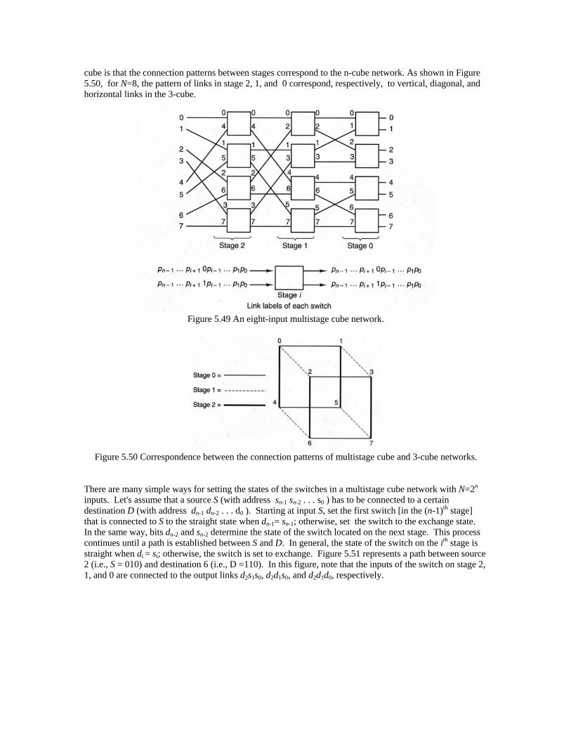
cube is that the connection patterns between stages correspond to the n-cube network. As shown in Figure 5.50, for N=8, the pattern of links in stage 2, 1, and 0 correspond, respectively, to vertical, diagonal, and horizontal links in the 3-cube.

Figure 5.49 An eight-input multistage cube network.

Figure 5.50 Correspondence between the connection patterns of multistage cube and 3-cube networks.

There are many simple ways for setting the states of the switches in a multistage cube network with N=2n inputs. Let's assume that a source S (with address sn-1 sn-2 . . . s0 ) has to be connected to a certain destination D (with address dn-1 dn-2 . . . d0 ). Starting at input S, set the first switch [in the (n-1)th stage] that is connected to S to the straight state when dn-1= sn-1; otherwise, set the switch to the exchange state. In the same way, bits dn-2 and sn-2 determine the state of the switch located on the next stage. This process continues until a path is established between S and D. In general, the state of the switch on the ith stage is straight when di = si; otherwise, the switch is set to exchange. Figure 5.51 represents a path between source 2 (i.e., S = 010) and destination 6 (i.e., D =110). In this figure, note that the inputs of the switch on stage 2, 1, and 0 are connected to the output links d2s1s0, d2d1s0, and d2d1d0, respectively.

Figure 5.51 Routing in a multistage cube.

In the preceding method the differences between the source and destination addresses can be stored as a tag, T, in the head of the packet. That is, T = S D = tn-1 . . . t0 determines the state of the switches on the path from source to destination. Once the packet arrives at a switch in stage i, the switch examines ti and sets its state. If ti=0, the switch is set in the straight state; otherwise, it is set in the exchange state. Another way is to add destination D as a tag to the header. In this way, the input of the switch on the ith stage is connected to the upper output when di = 0, otherwise, to the lower output. A multistage cube supports up to N one-to-one simultaneous connections. However, there are some permutations that cannot be established by this kind of network. For example, as shown in Figure 5.51, a permutation that requires source 3 and 7 to be connected to destinations 1 and 0, respectively, cannot be established. In addition to one-to-one connections, the multistage cube also supports one-to-many connections; that is, an input device can broadcast to all or a subset of the output devices. For example, Figure 5.52 represents the state of some switches for broadcasting from input 2 to outputs 4, 5, 6, and 7.

Figure 5.52 Broadcasting in a multistage cube.

Omega Network. The omega network was originally proposed by Lawrie [LAW 75] as an interconnection network between processors and memories. The network allows conflict-free access to rows, columns, diagonals, and square blocks of matrices [LAW 75]. This is important for matrix computation. The omega network provides the necessary permutations (for certain applications) at a substantially lower cost than a crossbar, since the omega requires fewer switches. The omega network consists of n = log2 N stages, where N is the number of inputs (outputs). Each stage in the network consists of a shuffle pattern of links followed by a column of N/2 switches. As an example, Figure 5.53 represents an omega network when N=8. Similar to the multistage cube, each switch has two inputs, two outputs, and four possible connection states (see Figure 5.48). Each switch is controlled individually. There is an efficient routing algorithm for setting the states of the switches in the omega

network. Let's assume that a source S (with address sn-1 sn-2 . . . s0 ) has to be connected to a certain destination D (with address dn-1 dn-2 . . . d0 ). Starting at input S, connect the input of the first switch [in the (n-1)th stage] that is connected to S to the upper output of the switch when dn-1= 0; otherwise, to the lower output. In the same way, bit dn-2 determines the output of the switch located on the next stage. This process continues until a path is established between S and D. In general, the input of the switch on the ith stage is connected to the upper output when di = 0; otherwise, the switch is connected to the lower output. Figure 5.53 represents a path between source 2 (i.e., S = 010) and destination 6 (i.e., D =110). The omega network is a blocking network; that is, some permutations cannot be established by the network. In Figure 5.53, for example, a permutation that requires sources 3 and 7 to be connected to destinations 1 and 0, respectively, cannot be established. However, such permutations can be established in several passes through the network. In other words, sometimes packets may need to go through several nodes so that a particular permutation can be established. For example, when node 3 is connected to node 1, node 7 can be connected to node 0 through node 4. That is, node 7 sends its packet to node 4, and then node 4 sends the packet to node 0. Therefore, we can connect node 3 to node 1 in one pass and node 7 to node 0 in two passes. In general, if we consider a single-stage shuffle-exchange network with N nodes, then every arbitrary permutation can be realized by passing through this network at most 3(log2N)-1 times [WU 81]. In addition to one-to-one connections, the omega network also supports broadcasting. Similar to the multistage cube network, the omega network can be used to broadcast data from one source to many destinations by setting some of the switches to the upper broadcast or lower broadcast state.

Figure 5.53 An eight-input omega network.

In general, the omega network is equivalent to a multistage cube network; that is, both provide the same set of permutations. In fact, some argue that the omega network is nothing more than an alias for a multistage cube network. Figure 5.54 demonstrates, for N=8, why this assertion may be true. By switching the position of switches 2 and 3 in stage 1 of the multistage cube network, the omega network can be obtained.

Figure 5.54 Mapping (a) a multistage cube network to (b) an omega network.

Another way to show equivalency (under certain assumptions) between the omega and multistage cube networks is through the representation of allowable permutations for each of them. Any permutation in a network with N inputs, where N=2n, can be expressed as a collection of n switching (Boolean) functions. For example, consider the following permutation for N=8:

[(0,0),(1,2),(2,4),(3,6),(4,1),(5,3),(6,5),(7,7)].

Let X=x2x1x0 denote the binary representation of a source. Also, let F(X)=f2f1f0 denote the binary representation of the destination that X is connected to. Then, the preceding permutation can be represented as follows: X connected to F(X) ___________________________________________________________ x2 x1 x0 f2 f1 f0 ___________________________________________________________ 0 0 0 0 0 0 0 0 1 0 1 0 0 1 0 1 0 0 0 1 1 1 1 0 1 0 0 0 0 1 1 0 1 0 1 1 1 1 0 1 0 1 1 1 1 1 1 1 ___________________________________________________________ Each of the switching functions f0, f1, and f2, therefore, can be expressed as

,212120 xxxxxf

,002021 xxxxxf

.112122 xxxxxf

Thus, in general, every permutation can be represented in terms of a set of switching functions. In the following, the switching representation of omega and multistage cube networks is derived. Initially, representations of basic functions, such as shuffle and exchange, are derived. These functions are then used to derive representations of omega and multistage cube networks. Shuffle ( ). The shuffle function is defined as

(xn-1 xn-2 . . . x0 ) = xn-2 xn-3 ... x0 xn-1. This function can also be represented as a set of switching functions, such as

11

0

1

1

nix

ixf

i

ni

Exchange (E). The exchange function E is defined as

.)( 021021 xxxxxxE nnnn

This function can also be represented as a set of switching functions, such as

11

00

nix

ixfi

i

Omega Network ( ). Recall that the omega network with n stages is a sequence of n shuffle-exchange functions. That is, )).()))(((( EEE Thus, to determine to which destination a given source

X=xn-1xn-2....x1x0 is connected, we must first apply function , then E, next again , and so on. As shown below, after applying and E n times to the source X, the switching functions can be obtained. First we apply :

.)( 102 xxxX nn

Next, we apply E to .102 xxx nn

,))(( 1102 cxxxXE nnn

where the bit cn-1 represents the control signal to the switches of the (n-1)th stage, and denotes the Boolean XOR function. It is assumed that one control signal ci goes to all the switches of the stage i, and each switch can have two states, straight (ci=0) and exchange (ci=1). Note that the bit xn-1 is exclusive-or’ed with cn-1, rather than complemented. This is because the bit cn-1 determines whether a switch is in the straight state or the exchange state, if a switch is in exchange state then the exchange function should be applied. Now we apply and then E to cxxx nnn 1102

,))))(((( 22113 cxcxxXEE nnnnn

where the bit cn-2 represents the control signal to the switches of the (n-2)th stage. Finally,

cxcxcxX nn .001111)(

Thus cxf iii for 10 ni

Multistage cube (C). The multistage cube can be represented as )),())))((((( 20 EEEC n

where i represents the connection between the switches of stage i+1 and i, and n is the number of stages.

Then function i is defined as

.)( 10210121 xxxxxxxx inninni

First we apply and then E .))(( 1102 cxxxXE nnn

where the bit cn-1 represents the control signal to the switches of the (n-1)th. It is assumed that one control

signal ci goes to all the switches of stage i, and each switch can have two states, straight (ci=0) and exchange (ci=1).

,))))(((( 2203112 cxxxcxXEE nnnnnn

.))))))(((((( 3304221123 cxxxcxcxXEEE nnnnnnnnn

Finally, )(XC cxcxcx nnnn .002211

Thus cxf iii for .10 ni

Note that the omega network also has the same set of switching functions; therefore, it is equivalent to the multistage cube. 5.3 INTERCONNECTION DESIGN DECISIONS A major problem in parallel computer design is finding an interconnection network capable of providing fast and efficient communication at a reasonable cost. There are at least five design considerations when selecting the architecture of an interconnection network: operation mode, switching methodology, network topology, a control strategy, and the functional characteristics of the switch. Operation mode. Three primary operating modes are available to the interconnection network designer: synchronous, asynchronous, and combined. When a synchronous stream of instructions or data is required by the network, a synchronous communication system is required. In other words, synchronous communication is needed for establishing communication paths synchronously for either data manipulating functions or for a data instruction broadcast. Most SIMD machines operate in a lock-step fashion; that is, all active processing nodes transmit data at the same time. Thus synchronous communication seems an appropriate choice for SIMD machines. When connection requests for an interconnection network are issued dynamically, an asynchronous communication system is needed. Since the timing of the routing requests is not predictable, the system must be able to handle such requests at any time. Some systems are designed to handle both synchronous and asynchronous communications. Such systems are able to do array processing by utilizing synchronous communications, yet are also able to control less predictable communication requests by using asynchronous timing methods. Switching methodology. The three main types of switching methodologies are circuit switching, packet switching, and integrated switching. Circuit switching establishes a complete path between source and destination and holds this path for the entire transmission. It is best suited for transmitting large amounts of continuous data. In contrast to circuit switching, packet switching has no dedicated physical connection set up. Hence it is most useful for transmitting small amounts of data. In packet switching, data items are partitioned into fixed-size packets. Each packet has a header that contains routing information, and moves from one node in the network to the next. The packet switching increases channel throughput by multiplexing various packets through the same path. Most SIMD machines use circuit switching, while packet switching is most suited to MIMD machines. The third option, integrated switching, is a combination of circuit and packet switching. This allows large amounts of data to be moved quickly over the physical path while allowing smaller packets of information to be transmitted via the network. Network topology. To design or select a topology, several performance parameters should be considered. The most important parameters are the following.

1. VLSI implementable. The topology of the network should be able to be mapped on two (or three) physical dimensions so that it can produce an efficient layout for packaging and implementation in

VLSI systems. 2. Small diameter. the diameter of the network should grow slowly with the number of nodes. 3. Neighbor independency. The number of neighbors of any node should be independent of the size

of the network. This allows the network to scale up to a very large size. 4. Easy to route. There should be an efficient algorithm for routing messages from any node to any

other. The messages must find an optimal path between the source and destination nodes and make use of all of the available bandwidth.

5. Uniform load. The traffic load on various parts of the network should be uniform. 6. Redundant Pathways. The network should be highly reliable and highly available. Message

pathways should be redundant to provide robustness in the event of component failure. Control strategy and functional characteristics of the switch. All dynamic networks are composed of switch boxes connected together through a series of links. The functional characteristics of a switch box are its size, routing logic, the number of possible states for the switch, fault detection and correction, communication protocols, and the amount of buffer space available for storing packets when there is congestion. Most of the switches provide some of these capabilities, depending on implementation requirements relating to efficiency and cost. In general, states of the switches of a network can be set by a central controller or by each individual switch. The former is a centralized control system, while the latter is a distributed one. Centralized control can be further broken down into individual stage control, individual box control, and partial stage control. Individual stage control uses one control signal to set all switch boxes at the same stage. Individual box control uses a separate control signal to set the state of each switch box. This offers higher flexibility in setting up the connecting paths, but increases the number of control signals, which, in turn, significantly increases control circuit complexity. In partial stage control, i+1 control signals are used at stage i of the network. In a distributed control network, the switches are usually more complex. In multistage interconnection networks, the switches have to deal with conflict resolution, as well as with changes in routing due to faults or congestion. Switches utilize protocols for handshaking to ensure that data may be correctly transferred. Large buffers enable a switch to store data that cannot be sent forward due to congestion. This allows increased performance of the network by decreasing the number of retransmissions.