Embed Size (px)
Citation preview

5. Hypothesis Testing
Dave Goldsman
Georgia Institute of Technology, Atlanta, GA, USA
8/21/10
Goldsman 8/21/10 1 / 64

Outline
1 Introduction to Hypothesis Testing
2 Normal Mean Tests (variance known)Simple Hypothesis TestTest DesignTwo-Sample Normal Mean Tests
3 Normal Mean Tests (variance unknown)Simple Hypothesis TestTwo-Sample Normal Mean Tests
Pooled t-TestApproximate t-TestPaired t-Test
4 Other Hypothesis TestsNormal Variance TestTwo-Sample Test for Equal VariancesBernoulli Proportion Test
Goldsman 8/21/10 2 / 64

Introduction to Hypothesis Testing
Introduction to Hypothesis Testing
General Approach
1. State a hypothesis.
2. Select a test statistic (to test whether or not the hypothesis is true).
3. Evaluate (calculate) the test statistic.
4. Interpret results — does the test statistic allow you to reject yourhypothesis?
Details follow. . .
Goldsman 8/21/10 3 / 64

Introduction to Hypothesis Testing
1. Hypotheses are simply statements or claims about parametervalues.
You perform a hypothesis test to prove or disprove the claim.
Set up a null hypothesis (H0) and an alternative hypothesis (H1) tocover the entire parameter space. The null hyp sort of represents the“status quo”.
Example: We claim that the mean weight of a filled package of chickenis µ0 ounces. (We specify µ0.)
H0 : µ = µ0
H1 : µ 6= µ0
This is a two-sided test . We’ll reject the claim if µ (an estimator of µ)is “too high” or “too small”.
Goldsman 8/21/10 4 / 64

Introduction to Hypothesis Testing
Example: We claim that a certain brand of tires lasts for at least amean of µ0 miles. (We specify µ0.)
H0 : µ ≥ µ0
H1 : µ < µ0
This is a one-sided test . We’ll reject the claim if µ is “too small”.
Example: We claim that emissions from a certain type of car do notexceed a mean of µ0 ppm. (We specify µ0.)
H0 : µ ≤ µ0
H1 : µ > µ0
This is a one-sided test . We’ll reject the claim if µ is “too large”.
Goldsman 8/21/10 5 / 64

Introduction to Hypothesis Testing
Idea: H0 is the old, conservative “status quo”. H1 is the new, radicalhypothesis. Although you may not be toooo sure about the truth of H0,you won’t reject it in favor of H1 unless you see substantial evidence insupport of H1.
“Innocent until proven guilty.”
If you get substantial evidence supporting H1, you’ll decide to rejectH0. Otherwise, you “fail to reject” H0. (This roughly means that yougrudgingly accept H0.)
Goldsman 8/21/10 6 / 64

Introduction to Hypothesis Testing
2. Select a test statistic (to test if H0 is true).
For instance, we could compare an estimator µ with µ0. Thecomparison is accomplished using a known sampling distribution (aka“test statistic”), e.g.,
zobs =X − µ0
σ/√
n(if σ2 is known) or
tobs =X − µ0
S/√
n(if σ2 is unknown)
Lots more details later.
Goldsman 8/21/10 7 / 64

Introduction to Hypothesis Testing
3. Evaluate the test statistic. Here’s the logic of hypothesis testing:
(a) Collect sample data(b) Assume H0 (the “status quo”) is true.(c) Determine the probability of the sample result, assuming H0 is true.(d) Decide from (c) if H0 is plausible.
* If the prob from (c) is low, reject H0 and select H1.* If the prob from (c) is high, fail to reject H0.
Goldsman 8/21/10 8 / 64

Introduction to Hypothesis Testing
Example: Time to metabolize a drug. Current drug takes µ0 = 15 min.Is new drug better?
Claim: Expected time for new drug is < 15 min.
H0 : µ ≥ 15
H1 : µ < 15
Data: n = 20, X = 14.88, S = 0.333. The test statistic is
tobs =X − µ0
S/√
n= −1.61.
Goldsman 8/21/10 9 / 64

Introduction to Hypothesis Testing
Now, if H0 is actually the true state of things, then µ = µ0, and from ourdiscussion on CI’s, we have
tobs =X − µ0
S/√
n∼ t(n − 1) ∼ t(19).
What would cause us to reject H0?
If X ≪ µ0(= 15), this would indicate that H0 is probably wrong.
Equivalently, I’d reject H0 if tobs is “significantly” ≪ 0.
Goldsman 8/21/10 10 / 64

Introduction to Hypothesis Testing
4. Interpret the Test Statistic.
So if H0 is true, is it reasonable (or, at least, not outrageous) to havegotten tobs = −1.61?
If yes, then we we’ll fail to reject H0.
If no, then we’ll reject H0 in favor of H1.
Goldsman 8/21/10 11 / 64

Introduction to Hypothesis Testing
Let’s see. . . . From the t table, we have
t0.05,19 = −1.729 and t0.10,19 = −1.328.
I.e.,P (t(19) < −1.729) = 0.05 and
P (t(19) < −1.328) = 0.10.
This means that
0.05 < p ≡ P (t(19) < −1.61︸ ︷︷ ︸
tobs
) < 0.10.
Goldsman 8/21/10 12 / 64

Introduction to Hypothesis Testing
In English: If H0 were true, there’s a 100p% chance that we’d see avalue of tobs that’s ≤ −1.61. That’s not a real high probability, but it’snot toooo small.
Formally, we’d reject H0 at “level” 0.10, sincetobs = −1.61 < t0.10,19 = −1.328.
But, we’d fail to reject H0 at level 0.05, sincetobs = −1.61 > t0.05,19 = −1.729.
More on this pretty soon!
Goldsman 8/21/10 13 / 64

Introduction to Hypothesis Testing
Where Can We Go Wrong? Four things can happen:
1. If H0 is actually true and we conclude that it’s true — good.
2. If H0 is actually false and we conclude that it’s false — good.
3. If H0 is actually true and we conclude that it’s false — bad. This iscalled Type I error .
Example: We conclude that a new, inferior drug is better than the drugcurrently on the market.
4. If H0 is actually false and we conclude that it’s true — bad. This iscalled Type II error .
Example: We conclude that a new, superior drug is worse than thedrug currently on the market.
Goldsman 8/21/10 14 / 64

Introduction to Hypothesis Testing
Want to keep
P (Type I error) = P (Reject H0 | H0 true) ≤ α
P (Type II error) = P (Fail to Rej H0 | H0 false) ≤ β
We choose α and β. Of course, we need to have α + β < 1.
Usually, Type I error is considered as “worse” than Type II.
Definition: The power of a hypothesis test is
1 − β = P (Reject H0 | H0 false).
It’s good to have high power.
Definition: The probability of Type I error, α, is called the size or levelof significance of the test.
Goldsman 8/21/10 15 / 64

Normal Mean Tests (variance known)
Outline
1 Introduction to Hypothesis Testing
2 Normal Mean Tests (variance known)Simple Hypothesis TestTest DesignTwo-Sample Normal Mean Tests
3 Normal Mean Tests (variance unknown)Simple Hypothesis TestTwo-Sample Normal Mean Tests
Pooled t-TestApproximate t-TestPaired t-Test
4 Other Hypothesis TestsNormal Variance TestTwo-Sample Test for Equal VariancesBernoulli Proportion Test
Goldsman 8/21/10 16 / 64

Normal Mean Tests (variance known) Simple Hypothesis Test
Simple Hypothesis Test
Suppose that X1, . . . ,Xniid∼ Nor(µ, σ2), where σ2 is somehow known
(not very realistic).
Two-sided test:H0 : µ = µ0 vs. H1 : µ 6= µ0
We’ll use X to estimate µ. If X is “significantly different” than µ0, thenwe’ll reject H0. But how much is “significantly different”?
To answer this, define
Z0 ≡ X − µ0
σ/√
n.
If H0 is true, then Z0 ∼ Nor(0, 1), in which case
P (−zα/2 ≤ Z0 ≤ zα/2) = 1 − α.
Goldsman 8/21/10 17 / 64

Normal Mean Tests (variance known) Simple Hypothesis Test
A value of Z0 outside the interval [−zα/2, zα/2] is highly unlikely if H0 istrue. Therefore,
Reject H0 iff |Z0| > zα/2.
This assures us that
P (Type I error) = P (Reject H0 | H0 true) = α.
If |Z0| > zα/2, then we’re in the rejection region . (Also called criticalregion .)
If |Z0| ≤ zα/2, then we’re in the acceptance region .
Goldsman 8/21/10 18 / 64
Normal Mean Tests (variance known) Simple Hypothesis Test
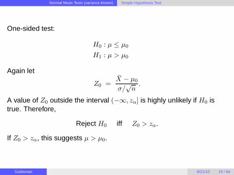
One-sided test:
H0 : µ ≤ µ0
H1 : µ > µ0
Again let
Z0 =X − µ0
σ/√
n.
A value of Z0 outside the interval (−∞, zα] is highly unlikely if H0 istrue. Therefore,
Reject H0 iff Z0 > zα.
If Z0 > zα, this suggests µ > µ0.
Goldsman 8/21/10 19 / 64

Normal Mean Tests (variance known) Simple Hypothesis Test
Similarly, the other one-sided test:
H0 : µ ≥ µ0
H1 : µ < µ0
A value of Z0 outside the interval [−zα,∞) is highly unlikely if H0 istrue. Therefore,
Reject H0 iff Z0 < −zα.
If Z0 < −zα, this suggests µ < µ0.
Goldsman 8/21/10 20 / 64

Normal Mean Tests (variance known) Simple Hypothesis Test
Example: We examine the weights of 25 nine-year-old kids. Supposewe somehow know that the weights are normally distributed withσ = 4. The sample mean of the 25 weights is 42.
Test the hypothesis that the mean weight is 40. Keep the probability ofType I error = 0.05.
H0 : µ = µ0 vs. H1 : µ 6= µ0
Here we have
Z0 =X − µ0
σ/√
n=
42 − 40
4/√
25= 2.5.
Since |Z0| = 2.5 > zα/2 = z0.025 = 1.96, we reject H0.
Notice that a lower α results in a higher zα/2. Then it’s “harder” toreject H0. For instance, if α = 0.01, then z0.005 = 2.58, and we fail toreject H0 in the above example.
Goldsman 8/21/10 21 / 64
Normal Mean Tests (variance known) Simple Hypothesis Test
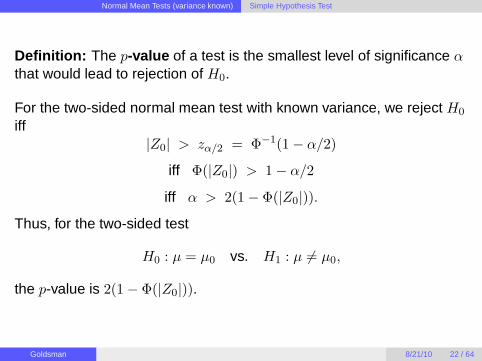
Definition: The p-value of a test is the smallest level of significance αthat would lead to rejection of H0.
For the two-sided normal mean test with known variance, we reject H0
iff|Z0| > zα/2 = Φ−1(1 − α/2)
iff Φ(|Z0|) > 1 − α/2
iff α > 2(1 − Φ(|Z0|)).Thus, for the two-sided test
H0 : µ = µ0 vs. H1 : µ 6= µ0,
the p-value is 2(1 − Φ(|Z0|)).
Goldsman 8/21/10 22 / 64

Normal Mean Tests (variance known) Simple Hypothesis Test
Similarly, for the one-sided test
H0 : µ ≤ µ0 vs. H1 : µ > µ0,
we have p = 1 − Φ(Z0).
And for the other one-sided test
H0 : µ ≥ µ0 vs. H1 : µ < µ0,
we have p = Φ(Z0).
Example: For the previous example,
p = 2(1 − Φ(|Z0|)) = 2(1 − Φ(2.5)) = 0.0124.
Goldsman 8/21/10 23 / 64

Normal Mean Tests (variance known) Test Design
Test Design
Can we design a two-sided test with the following constraints on Type Iand II errors?
P (Type I error) = α and
P (Type II error |µ = µ1 > µ0) = β
I.e., can we design a two-sided test that will work when we require aType I error bound α, and a Type II prob β (in the special case that thetrue mean µ happens to equal a user-specified value µ1 > µ0)?
Suppose the difference between the actual and hypothesized means is
δ ≡ µ − µ0 = µ1 − µ0.
(Without loss of generality, we’ll assume µ1 > µ0.) Then the α and βdesign requirements can be achieved by taking a sample of size
n ≈ σ2(zα/2 + zβ)2/δ2.
Goldsman 8/21/10 24 / 64
Normal Mean Tests (variance known) Test Design
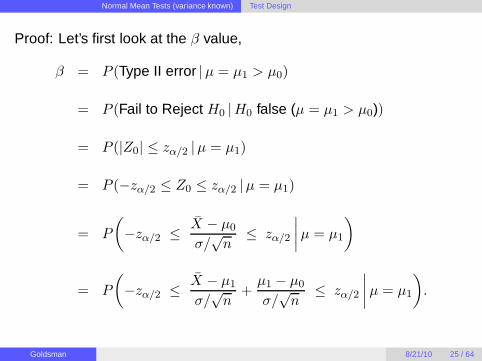
Proof: Let’s first look at the β value,
β = P (Type II error |µ = µ1 > µ0)
= P (Fail to Reject H0 |H0 false (µ = µ1 > µ0))
= P (|Z0| ≤ zα/2 |µ = µ1)
= P (−zα/2 ≤ Z0 ≤ zα/2 |µ = µ1)
= P
(
−zα/2 ≤ X − µ0
σ/√
n≤ zα/2
∣∣∣∣µ = µ1
)
= P
(
−zα/2 ≤ X − µ1
σ/√
n+
µ1 − µ0
σ/√
n≤ zα/2
∣∣∣∣µ = µ1
)
.
Goldsman 8/21/10 25 / 64

Normal Mean Tests (variance known) Test Design
Notice that
Z ≡ X − µ1
σ/√
n∼ Nor(0, 1).
This gives
β = P
(
−zα/2 ≤ Z +
√nδ
σ≤ zα/2
)
= P
(
−zα/2 −√
nδ
σ≤ Z ≤ zα/2 −
√nδ
σ
)
= Φ
(
zα/2 −√
nδ
σ
)
− Φ
(
−zα/2 −√
nδ
σ
)
.
Now, note that −zα/2 ≪ 0 and −√nδ/σ < 0 (since δ > 0).
These two facts imply that the second term in the expression for βabove is ≈ 0, so. . .
Goldsman 8/21/10 26 / 64

Normal Mean Tests (variance known) Test Design
We only need to use the first term in the previous expression for β:
β ≈ Φ
(
zα/2 −√
nδ
σ
)
iff
Φ−1(β) = −zβ ≈ zα/2 −√
nδ
σ
iff √nδ
σ≈ zα/2 + zβ
iffn ≈ σ2(zα/2 + zβ)2/δ2. Done!
Goldsman 8/21/10 27 / 64

Normal Mean Tests (variance known) Test Design
Recap: If you want to test H0 : µ = µ0 vs. H1 : µ 6= µ0, and(1) You know σ2,(2) You want P (Type I error) = α, and(3) You want P (Type II error) = β if µ = µ1(6= µ0),
then you have to take n ≈ σ2(zα/2 + zβ)2/δ2 observations.
Similarly, if you’re doing a one-sided test, it turns out that you need totake n ≈ σ2(zα + zβ)2/δ2 obsns.
Example: Weights of 9-yr-old kids are normal with σ = 4. How manyobsns should we take if we wish to test H0 : µ = 40 vs. H1 : µ 6= 40,and we want α = 0.05, and β = 0.05 if µ happens to actually equalµ1 = 42?
n ≈ σ2
δ2(zα/2 + zβ)2 =
16
4(1.96 + 1.645)2 = 51.98.
In other words, you need about 52 observations.
Goldsman 8/21/10 28 / 64

Normal Mean Tests (variance known) Two-Sample Normal Mean Tests
Two-Sample Normal Means Test (variances known)
Suppose we have the following set-up:
X1,X2, . . . ,Xniid∼ Nor(µx, σ2
x) and
Y1, Y2, . . . , Ymiid∼ Nor(µy, σ
2y),
where the samples are indep of each other, and σ2x and σ2
y aresomehow known.
Which population has the larger mean?
Here’s the two-sided test to see if the means are different.
H0 : µx = µy
H1 : µx 6= µy
Goldsman 8/21/10 29 / 64

Normal Mean Tests (variance known) Two-Sample Normal Mean Tests
Define the test statistic
Z0 =X − Y − (µx − µy)
√σ2
x
n +σ2
y
m
.
If H0 is true (i.e., the means are equal), then
Z0 =X − Y
√σ2
x
n +σ2
y
m
∼ Nor(0, 1).
Thus, as before,
Reject H0 iff |Z0| > zα/2.
Goldsman 8/21/10 30 / 64
Normal Mean Tests (variance known) Two-Sample Normal Mean Tests
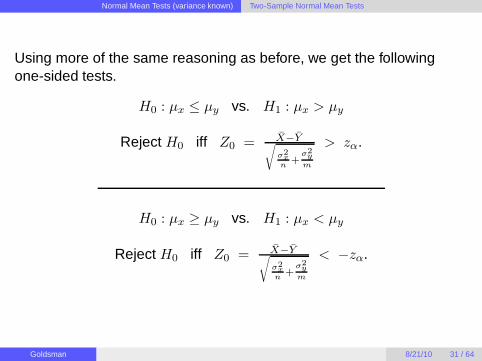
Using more of the same reasoning as before, we get the followingone-sided tests.
H0 : µx ≤ µy vs. H1 : µx > µy
Reject H0 iff Z0 = X−Y√
σ2x
n+
σ2y
m
> zα.
H0 : µx ≥ µy vs. H1 : µx < µy
Reject H0 iff Z0 = X−Y√
σ2x
n+
σ2y
m
< −zα.
Goldsman 8/21/10 31 / 64

Normal Mean Tests (variance known) Two-Sample Normal Mean Tests
Example: Suppose we want to test H0 : µx = µy vs. H1 : µx 6= µy, andwe have the following data:
n = 10, X = 824.9, σ2x = 40
m = 10, Y = 818.6, σ2y = 50
ThenZ0 =
824.9 − 818.6√
4010 + 50
10
= 2.10.
If α = 0.05, then |Z0| = 2.10 > zα/2 = 1.96, and so we reject H0.
Goldsman 8/21/10 32 / 64

Normal Mean Tests (variance unknown)
Outline
1 Introduction to Hypothesis Testing
2 Normal Mean Tests (variance known)Simple Hypothesis TestTest DesignTwo-Sample Normal Mean Tests
3 Normal Mean Tests (variance unknown)Simple Hypothesis TestTwo-Sample Normal Mean Tests
Pooled t-TestApproximate t-TestPaired t-Test
4 Other Hypothesis TestsNormal Variance TestTwo-Sample Test for Equal VariancesBernoulli Proportion Test
Goldsman 8/21/10 33 / 64

Normal Mean Tests (variance unknown) Simple Hypothesis Test
Simple Hypothesis Test
Suppose X1, . . . ,Xniid∼ Nor(µ, σ2), where σ2 is unknown.
Two-sided test:H0 : µ = µ0 vs. H1 : µ 6= µ0
We’ll use X to estimate µ. If X is “significantly different” than µ0, thenwe’ll reject H0. To determine what “significantly different” means, we’llalso need to estimate σ2.
Define the test statistic
T0 ≡ X − µ0
S/√
n,
where S2 is our old friend, the sample variance,
S2 ≡ 1
n − 1
n∑
i=1
(Xi − X)2 ∼ σ2χ2(n − 1)
n − 1.
Goldsman 8/21/10 34 / 64

Normal Mean Tests (variance unknown) Simple Hypothesis Test
If H0 is true, then
T0 =
X−µ0√σ2/n
√S2
σ2
∼ Nor(0, 1)√
χ2(n−1)n−1
∼ t(n − 1).
So
Reject H0 iff |T0| > tα/2,n−1.
One-Sided Tests:
H0 : µ ≤ µ0 vs. H1 : µ > µ0
Reject H0 iff T0 > tα,n−1.
H0 : µ ≥ µ0 vs. H1 : µ < µ0
Reject H0 iff T0 < −tα,n−1.
Goldsman 8/21/10 35 / 64

Normal Mean Tests (variance unknown) Simple Hypothesis Test
Example: Suppose we want to test at level 0.05 whether or not themean of some process is 150.
We have n = 15, X = 152.18, and S2 = 16.63.
Then
T0 ≡ X − µ0
S/√
n= 2.07.
Since tα/2,n−1 = t0.025,14 = 2.145, we fail to reject H0.
Goldsman 8/21/10 36 / 64

Normal Mean Tests (variance unknown) Two-Sample Normal Mean Tests
Two-Sample Normal Mean Tests when Variances are Unknown
Suppose we have the following set-up:
X1,X2, . . . ,Xniid∼ Nor(µx, σ2
x) and
Y1, Y2, . . . , Ymiid∼ Nor(µy, σ
2y),
where the samples are indep of each other, and σ2x and σ2
y areunknown.
Which population has the larger mean?
We’ll look at three cases:
Pooled t-test: σ2x = σ2
y = σ2, say.
Approximate t-test: σ2x 6= σ2
y.
Paired t-test: (Xi, Yi) observations paired.Goldsman 8/21/10 37 / 64

Normal Mean Tests (variance unknown) Two-Sample Normal Mean Tests
Pooled t-Test
Suppose that σ2x = σ2
y = σ2 (unknown).
Consider the two-sided test to see if the means are different.
H0 : µx = µy vs. H1 : µx 6= µy
Sample means and variances from the two popns:
X ≡ 1
n
n∑
i=1
Xi and Y ≡ 1
m
m∑
i=1
Yi
S2x =
∑ni=1(Xi − X)2
n − 1and S2
y =
∑mi=1(Yi − Y )2
m − 1.
Define the pooled variance estimator by
S2p =
(n − 1)S2x + (m − 1)S2
y
n + m − 2.
Goldsman 8/21/10 38 / 64

Normal Mean Tests (variance unknown) Two-Sample Normal Mean Tests
If H0 is true, it can be shown that
S2p ∼ σ2χ2(n + m − 2)
n + m − 2,
and then the test statistic
T0 ≡ X − Y
Sp
√1n + 1
m
∼ t(n + m − 2).
Thus,Reject H0 iff |T0| > tα/2,n+m−2.
Goldsman 8/21/10 39 / 64

Normal Mean Tests (variance unknown) Two-Sample Normal Mean Tests
One-Sided Tests:
H0 : µx ≤ µy vs. H1 : µx > µy
Reject H0 iff T0 > tα,n+m−2.
H0 : µx ≥ µy vs. H1 : µx < µy
Reject H0 iff T0 < −tα,n+m−2.
Example: Catalyst X is currently used by a certain chemical process.If catalyst Y gives higher mean yield, we’ll use it instead.
Thus, we want to test H0 : µx ≥ µy vs. H1 : µx < µy.
Suppose we have the following data:
n = 8, X = 91.73, S2x = 3.89
m = 8, Y = 93.75, S2y = 4.02
Goldsman 8/21/10 40 / 64
Normal Mean Tests (variance unknown) Two-Sample Normal Mean Tests
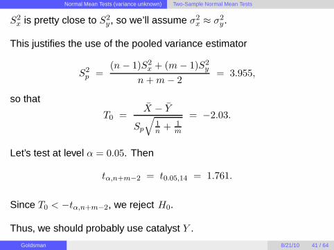
S2x is pretty close to S2
y , so we’ll assume σ2x ≈ σ2
y.
This justifies the use of the pooled variance estimator
S2p =
(n − 1)S2x + (m − 1)S2
y
n + m − 2= 3.955,
so that
T0 =X − Y
Sp
√1n + 1
m
= −2.03.
Let’s test at level α = 0.05. Then
tα,n+m−2 = t0.05,14 = 1.761.
Since T0 < −tα,n+m−2, we reject H0.
Thus, we should probably use catalyst Y .
Goldsman 8/21/10 41 / 64
Normal Mean Tests (variance unknown) Two-Sample Normal Mean Tests
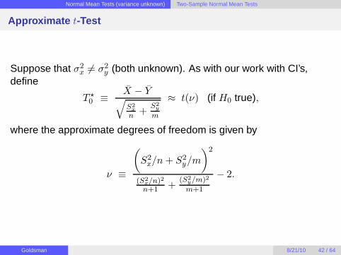
Approximate t-Test
Suppose that σ2x 6= σ2
y (both unknown). As with our work with CI’s,define
T ⋆0 ≡ X − Y
√S2
x
n +S2
y
m
≈ t(ν) (if H0 true),
where the approximate degrees of freedom is given by
ν ≡
(
S2x/n + S2
y/m
)2
(S2x/n)2
n+1 +(S2
y/m)2
m+1
− 2.
Goldsman 8/21/10 42 / 64

Normal Mean Tests (variance unknown) Two-Sample Normal Mean Tests
2-sided H0 : µx = µy Reject H0 iff |T ⋆0 | > tα/2,ν
H1 : µx 6= µy
1-sided H0 : µx ≤ µy Reject H0 iff T ⋆0 > tα,ν
H1 : µx > µy
1-sided H0 : µx ≥ µy Reject H0 iff T ⋆0 < −tα,ν
H1 : µx < µy
Goldsman 8/21/10 43 / 64

Normal Mean Tests (variance unknown) Two-Sample Normal Mean Tests
Example: Let’s test H0 : µx = µy vs. H1 : µx 6= µy at level α = 0.10.
Suppose we have the following data:
n = 15, X = 24.2, S2x = 10
m = 10, Y = 23.9, S2y = 20
S2x isn’t very close to S2
y , so we’ll assume σ2x 6= σ2
y .
Plug-and-chug to getT ⋆
0 = 0.184,
ν = 16.2 → 16,
tα/2,ν = t0.05,16 = 1.746.
Since |T ⋆0 | < tα/2,ν , we fail to reject H0. (Actually, T ⋆
0 was so close to 0,we didn’t need the tables.)
Goldsman 8/21/10 44 / 64

Normal Mean Tests (variance unknown) Two-Sample Normal Mean Tests
Paired t-Test
Again consider two competing normal pop’ns. Suppose we collectobs’ns from the two pop’ns in pairs.
The RV’s within different pairs are indep. The two obs’ns within thesame pair may not be indep — in fact, it’s good for them to bepositively correlated!
Example: One twin takes a new drug, the other takes a placebo.
indep
Pair 1 : (X1, Y1)
Pair 2 : (X2, Y2)...
...
Pair n : (Xn, Yn)︸ ︷︷ ︸
not indep
Goldsman 8/21/10 45 / 64
Normal Mean Tests (variance unknown) Two-Sample Normal Mean Tests
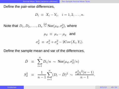
Define the pair-wise differences,
Di ≡ Xi − Yi, i = 1, 2, . . . , n.
Note that D1,D2, . . . ,Dniid∼ Nor(µd, σ
2d), where
µd ≡ µx − µy and
σ2d ≡ σ2
x + σ2y − 2Cov(Xi, Yi).
Define the sample mean and var of the differences,
D ≡n∑
i=1
Di/n ∼ Nor(µd, σ2d/n)
S2d ≡ 1
n − 1
n∑
i=1
(Di − D)2 ∼ σ2dχ
2(n − 1)
n − 1.
Goldsman 8/21/10 46 / 64

Normal Mean Tests (variance unknown) Two-Sample Normal Mean Tests
Then the test statistic is (assuming µd = 0)
T0 ≡ D√
S2d/n
∼ t(n − 1).
Using the exact same manipulations as in the single-sample normalmean problem with unknown variance, we get the following. . .
2-sided H0 : µd = 0 Reject H0 iff |T0| > tα/2,n−1
H1 : µd 6= 0
1-sided H0 : µd ≤ 0 Reject H0 iff T0 > tα,n−1
H1 : µd > 0
1-sided H0 : µd ≥ 0 Reject H0 iff T0 < −tα,n−1
H1 : µd < 0
Recall µd = µx − µy, so that, e.g., µd = 0 iff µx = µy.
Goldsman 8/21/10 47 / 64
Normal Mean Tests (variance unknown) Two-Sample Normal Mean Tests
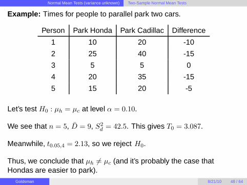
Example: Times for people to parallel park two cars.
Person Park Honda Park Cadillac Difference
1 10 20 -10
2 25 40 -15
3 5 5 0
4 20 35 -15
5 15 20 -5
Let’s test H0 : µh = µc at level α = 0.10.
We see that n = 5, D = 9, S2d = 42.5. This gives T0 = 3.087.
Meanwhile, t0.05,4 = 2.13, so we reject H0.
Thus, we conclude that µh 6= µc (and it’s probably the case thatHondas are easier to park).
Goldsman 8/21/10 48 / 64

Other Hypothesis Tests
Outline
1 Introduction to Hypothesis Testing
2 Normal Mean Tests (variance known)Simple Hypothesis TestTest DesignTwo-Sample Normal Mean Tests
3 Normal Mean Tests (variance unknown)Simple Hypothesis TestTwo-Sample Normal Mean Tests
Pooled t-TestApproximate t-TestPaired t-Test
4 Other Hypothesis TestsNormal Variance TestTwo-Sample Test for Equal VariancesBernoulli Proportion Test
Goldsman 8/21/10 49 / 64

Other Hypothesis Tests Normal Variance Test
Normal Variance Test
Suppose X1, . . . ,Xniid∼ Nor(µ, σ2), where µ and σ2 are unknown.
Two-sided test (you specify hypothesized σ20):
H0 : σ2 = σ20 vs. H1 : σ2 6= σ2
0
We’ll use the test statistic
χ20 ≡ (n − 1)S2
σ20
∼ χ2(n − 1) (if H0 true),
where
S2 ≡ 1
n − 1
n∑
i=1
(Xi − X)2 ∼ σ2χ2(n − 1)
n − 1.
Thus, we reject H0 iff
χ20 < χ2
1−α/2,n−1 or χ20 > χ2
α/2,n−1.
Goldsman 8/21/10 50 / 64

Other Hypothesis Tests Normal Variance Test
One-Sided Tests:
H0 : σ2 ≤ σ20 vs. H1 : σ2 > σ2
0
Reject H0 iff χ20 > χ2
α,n−1.
H0 : σ2 ≥ σ20 vs. H1 : σ2 < σ2
0
Reject H0 iff χ20 < χ2
1−α,n−1.
Example: Suppose we want to test at level 0.05 whether or not thevariance of a certain process is ≤ 0.02.
H0 : σ2 ≤ 0.02 vs. H1 : σ2 > 0.02
If the sample variance is “too high”, we’ll reject H0.
Goldsman 8/21/10 51 / 64

Other Hypothesis Tests Normal Variance Test
Suppose we have n = 20, X = 125.12, and S2 = 0.00225.
Then the test stat χ20 = (n − 1)S2/σ2
0 = 21.375 (and isn’t explicitlydependent on X).
Further, χ2α,n−1 = χ2
0.05,19 = 30.14.
So we fail to reject H0.
Goldsman 8/21/10 52 / 64

Other Hypothesis Tests Two-Sample Test for Equal Variances
Two-Sample Test for Equal Variances
Do the two populations have the same variance?
X1,X2, . . . ,Xniid∼ Nor(µx, σ2
x) and
Y1, Y2, . . . , Ymiid∼ Nor(µy, σ
2y).
All X ’s and Y ’s are independent.
Two-sided test: H0 : σ2x = σ2
y vs. H1 : σ2x 6= σ2
y
Goldsman 8/21/10 53 / 64

Other Hypothesis Tests Two-Sample Test for Equal Variances
We’ll use the test statistic
F0 ≡ S2x
S2y
∼ F (n − 1,m − 1) (if H0 true),
where S2x and S2
y are the two sample variances.
Thus, we reject H0 iff
F0 < F1−α/2,n−1,m−1 or F0 > Fα/2,n−1,m−1.
iffF0 <
1
Fα/2,m−1,n−1or F0 > Fα/2,n−1,m−1.
Goldsman 8/21/10 54 / 64

Other Hypothesis Tests Two-Sample Test for Equal Variances
One-Sided Tests:
H0 : σ2x ≤ σ2
y vs. H1 : σ2x > σ2
y
Reject H0 iff F0 > Fα,n−1,m−1.
H0 : σ2x ≥ σ2
y vs. H1 : σ2x < σ2
y
Reject H0 iff F0 < F1−α,n−1,m−1 = 1Fα,m−1,n−1
.
Goldsman 8/21/10 55 / 64

Other Hypothesis Tests Two-Sample Test for Equal Variances
Example: Suppose we want to test at level 0.05 whether or not twoprocesses have the same variance.
H0 : σ2x = σ2
y vs. H1 : σ2x 6= σ2
y
If the ratio of the sample variances is “too high” or “too low”, reject H0.
Suppose we have the following data:
n = m = 8, S2x = 3.89, S2
y = 4.02.
Then F0 = S2x/S2
y = 0.968,
F1−α/2,n−1,m−1 = 1/F0.025,7,7 = 0.20, and
Fα/2,n−1,m−1 = F0.025,7,7 = 4.99.
Thus, we fail to reject H0.
Goldsman 8/21/10 56 / 64

Other Hypothesis Tests Bernoulli Proportion Test
Bernoulli Proportion Test
Suppose that X1,X2, . . . ,Xniid∼ Bern(p).
We’re interested in testing hypotheses about the success parameter p.
Two-sided test (you specify hypothesized p0):
H0 : p = p0 vs. H1 : p 6= p0
Let Y =∑n
i=1 Xi ∼ Bin(n, p).
We’ll use the test statistic
Z0 ≡ Y − np0√
np0(1 − p0).
If H0 is true, the central limit theorem implies that
Z0 ≈ Nor(0, 1).
Goldsman 8/21/10 57 / 64

Other Hypothesis Tests Bernoulli Proportion Test
Thus, we reject H0 iff |Z0| > zα/2.
Tips: In order for the CLT to work, you need n large (say at least 30),and p not too close to 0 or 1.
Remark: If n isn’t very big, you may have to use Binomial tables(instead of the normal approxn). This gets a little tedious, and I won’tgo into it here!
One-Sided Tests:
H0 : p ≤ p0 vs. H1 : p > p0
Reject H0 iff Z0 > zα.
H0 : p ≥ p0 vs. H1 : p < p0
Reject H0 iff Z0 < −zα.
Goldsman 8/21/10 58 / 64

Other Hypothesis Tests Bernoulli Proportion Test
Example: In 200 samples of a certain semiconductor, there were only4 defectives. We’re interested in proving “beyond a shadow of a doubt”that the probability of a defective is less than 0.06. Let’s conduct thetest at level 0.05.
H0 : p ≥ 0.06 vs. H1 : p < 0.06
(Since p is close to 0, we really did need to take a lot of observations— 200 in this case — in order for the CLT to work.)
We have n = 200, Y = 4 defectives, and p0 = 0.06.
The test stat is
Z0 =Y − np0
√
np0(1 − p0)= −2.357.
Since −zα = −1.645, we reject H0. I.e., it looks like p really is < 0.06.
Goldsman 8/21/10 59 / 64

Other Hypothesis Tests Bernoulli Proportion Test
Sample-Size Selection
Can we design a two-sided test H0 : p = p0 vs. H1 : p 6= p0 such that
P (Type I error) = α and P (Type II error | p 6= p0) = β?
I.e., can we specify the sample size for a two-sided test that will workwhen we require a Type I error bound α, and a Type II prob β?
Yes! We’ll now show that the necessary sample size is
n ≈[zα/2
√p0q0 + zβ
√pq
p − p0
]2
,
where, to save space, we let q ≡ 1 − p and q0 ≡ 1 − p0.
Notice that n is a function of the unknown p. In practice, we’ll choosesome p = p1 and ask “How many obsns should I take if p happens toequal p1 instead of p0”? Thus, we guard against the scenario in whichp actually equals p1.
Goldsman 8/21/10 60 / 64
Other Hypothesis Tests Bernoulli Proportion Test
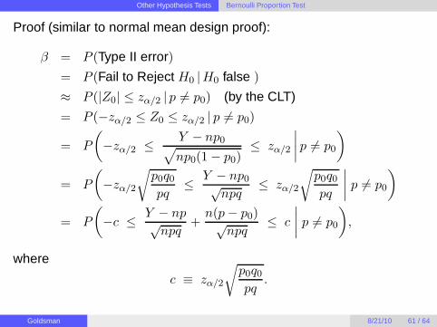
Proof (similar to normal mean design proof):
β = P (Type II error)
= P (Fail to Reject H0 |H0 false )
≈ P (|Z0| ≤ zα/2 | p 6= p0) (by the CLT)
= P (−zα/2 ≤ Z0 ≤ zα/2 | p 6= p0)
= P
(
−zα/2 ≤ Y − np0√
np0(1 − p0)≤ zα/2
∣∣∣∣p 6= p0
)
= P
(
−zα/2
√p0q0
pq≤ Y − np0√
npq≤ zα/2
√p0q0
pq
∣∣∣∣p 6= p0
)
= P
(
−c ≤ Y − np√npq
+n(p − p0)√
npq≤ c
∣∣∣∣p 6= p0
)
,
where
c ≡ zα/2
√p0q0
pq.
Goldsman 8/21/10 61 / 64

Other Hypothesis Tests Bernoulli Proportion Test
Now notice that (since p is the true success prob),
Z ≡ Y − np√npq
≈ Nor(0, 1).
This gives
β ≈ P
(
−c ≤ Z +n(p − p0)√
npq≤ c
)
= P
(
−c −√
n(p − p0)√pq
≤ Z ≤ c −√
n(p − p0)√pq
)
= P (−c − d ≤ Z ≤ c − d)
= Φ(c − d) − Φ(−c − d),
where
d ≡√
n(p − p0)√pq
.
Goldsman 8/21/10 62 / 64

Other Hypothesis Tests Bernoulli Proportion Test
Also notice that
−c − d = −zα/2
√p0q0
pq−
√n(p − p0)√
pq≪ 0.
This implies, Φ(−c − d) ≈ 0, and so. . .
β ≈ Φ(c − d) iff c − d ≈ Φ−1(β) = −zβ
iff
−zβ ≈ zα/2
√p0q0
pq−
√n(p − p0)√
pq.
After a little algebra, we finally(!) get
n ≈[zα/2
√p0q0 + zβ
√pq
p − p0
]2
.
Similarly, the sample size for the corresponding one-sided test is
n ≈[zα
√p0q0 + zβ
√pq
p − p0
]2
.
Goldsman 8/21/10 63 / 64

Other Hypothesis Tests Bernoulli Proportion Test
Stuff still to add to notes
Numerical example for binomial hyp test design.
More material on power function.
χ2 goodness-of-fit test; contingency tables.
Goldsman 8/21/10 64 / 64