Embed Size (px)
Citation preview
5
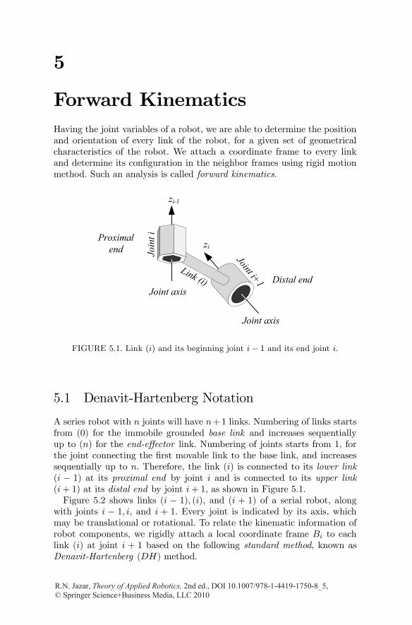
Forward KinematicsHaving the joint variables of a robot, we are able to determine the positionand orientation of every link of the robot, for a given set of geometricalcharacteristics of the robot. We attach a coordinate frame to every linkand determine its configuration in the neighbor frames using rigid motionmethod. Such an analysis is called forward kinematics.
zi
Link (i)
zi-1
Joint i+1Jo
int i
Joint axis
Joint axis
Proximal end
Distal end
FIGURE 5.1. Link (i) and its beginning joint i− 1 and its end joint i.
5.1 Denavit-Hartenberg Notation
A series robot with n joints will have n+1 links. Numbering of links startsfrom (0) for the immobile grounded base link and increases sequentiallyup to (n) for the end-effector link. Numbering of joints starts from 1, forthe joint connecting the first movable link to the base link, and increasessequentially up to n. Therefore, the link (i) is connected to its lower link(i − 1) at its proximal end by joint i and is connected to its upper link(i+ 1) at its distal end by joint i+ 1, as shown in Figure 5.1.Figure 5.2 shows links (i − 1), (i), and (i + 1) of a serial robot, along
with joints i − 1, i, and i + 1. Every joint is indicated by its axis, whichmay be translational or rotational. To relate the kinematic information ofrobot components, we rigidly attach a local coordinate frame Bi to eachlink (i) at joint i + 1 based on the following standard method, known asDenavit-Hartenberg (DH) method.
R.N. Jazar, Theory of Applied Robotics, 2nd ed., DOI 10.1007/978-1-4419-1750-8_5, © Springer Science+Business Media, LLC 2010
234 5. Forward Kinematics
1. The zi-axis is aligned with the i+ 1 joint axis.
All joints, without exception, are represented by a z-axis. We alwaysstart with identifying the zi-axes. The positive direction of the zi-axisis arbitrary. Identifying the joint axes for revolute joints is obvious,however, a prismatic joint may pick any axis parallel to the directionof translation. By assigning the zi-axes, the pairs of links on eitherside of each joint, and also two joints on either side of each link arealso identified.
Although the zi-axes of two joints at the ends of a link can be skew,we make the industrial robots such that the zi-axes are parallel, per-pendicular, or orthogonal. Two parallel joint axes are indicated by aparallel sign, (k). Two joint exes are orthogonal if their axes are in-tersecting at a right angle. Orthogonal joint axes are indicated by anorthogonal sign, (`). Two joints are perpendicular if their axes areat a right angle with respect to their common normal. Perpendicularjoint axes are indicated by a perpendicular sign, (⊥).
2. The xi-axis is defined along the common normal between the zi−1and zi axes, pointing from the zi−1 to the zi-axis.
In general, the z-axes may be skew lines, however there is always oneline mutually perpendicular to any two skew lines, called the commonnormal. The common normal has the shortest distance between thetwo skew lines.
When the two z-axes are parallel, there are an infinite number ofcommon normals. In that case, we pick the common normal that iscollinear with the common normal of the previous joints.
When the two z-axes are intersecting, there is no common normalbetween them. In that case, we assign the xi-axis perpendicular tothe plane formed by the two z-axes in the direction of zi−1 × zi.
In case the two z-axes are collinear, the only nontrivial arrangementof joints is either PkR or RkP. Hence, we assign the xi-axis such thatwe have the joint variable equal to θi = 0 in the rest position of therobot.
3. The yi-axis is determined by the right-hand rule, yi = zi × xi.
Generally speaking, we assign reference frames to each link so thatone of the three coordinate axes xi, yi, or zi (usually xi) is alignedalong the axis of the distal joint.
By applying the DH method, the origin oi of the frame Bi(oi, xi, yi, zi),attached to the link (i), is placed at the intersection of the joint axis i+ 1with the common normal between the zi−1 and zi axes.A DH coordinate frame is identified by four parameters: ai, αi, θi, and
di.
5. Forward Kinematics 235
zi
Link (i)
Link
(i+
1)Joint i-1
zi-2
xi-1
yi-1
xiyi
oi
oi-1
Bi
Bi-2Bi-1
Link (i-1)
Joint i Join
t i+
1
zi-1
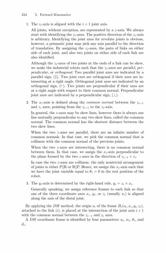
FIGURE 5.2. Links (i− 1), (i), and (i+1) along with coordinate frames Bi andBi+1.
1. Link length ai is the distance between zi−1 and zi axes along thexi-axis. ai is the kinematic length of link (i).
2. Link twist αi is the required rotation of the zi−1-axis about the xi-axis to become parallel to the zi-axis.
3. Joint distance di is the distance between xi−1 and xi axes along thezi−1-axis. Joint distance is also called link offset.
4. Joint angle θi is the required rotation of xi−1-axis about the zi−1-axisto become parallel to the xi-axis.
DH frame parameters of the links in Figure 5.2 are illustrated in Figure5.3. The parameters θi and di are called joint parameters, since they definethe relative position of two adjacent links connected at joint i. In a givendesign for a robot, each joint is revolute or prismatic. Thus, for each joint, itwill always be the case that either θi or di is fixed and the other is variable.For a revolute joint (R) at joint i, the value of di is fixed, while θi is theunique joint variable. For a prismatic joint (P), the value of θi is fixed anddi is the only joint variable. The variable parameter either θi or di is calledthe joint variable. The joint parameters θi and di define a screw motionbecause θi is a rotation about the zi−1-axis, and di is a translation alongthe zi−1-axis.The parameters αi and ai are called link parameters, because they define
relative positions of joints i and i + 1 at two ends of link (i). The link
236 5. Forward Kinematics
zi
Link (i)
Link
(i+
1)Joint i-1
zi-2
xi-1
xiyi
oi
oi-1
Bi
Bi-2
Bi-1
Link (i-1)
Joint i Join
t i+
1
zi-1
ai
di
iα
iθ
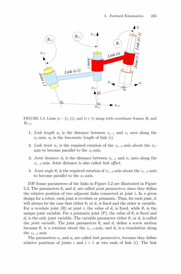
FIGURE 5.3. DH parameters ai, αi, di, θi defined for joint i and link (i).
twist αi is the angle of rotation zi−1-axis about xi to become parallel withthe zi-axis. The other link parameter, ai, is the translation along the xi-axis to bring the zi−1-axis on the zi-axis. The link parameters αi and aidefine a screw motion because αi is a rotation about the xi-axis, and ai isa translation along the xi-axis.In other words, we can move the zi−1-axis to the zi-axis by a central
screw s(ai, αi, ı), and move the xi−1-axis to the xi-axis by a central screws(di, θi, ki−1).
Example 134 Simplification comments for the DH method.There are some comments to simplify the application of the DH frame
method.
1. Showing only z and x axes is sufficient to identify a coordinate frame.Drawing is made clearer by not showing y axes.
2. If the first and last joints are R, then
a0 = 0 , an = 0 (5.1)
α0 = 0 , αn = 0. (5.2)
In these cases, the zero position for θ1, and θn can be chosen arbi-trarily, and link offsets can be set to zero.
d1 = 0 , dn = 0 (5.3)
5. Forward Kinematics 237
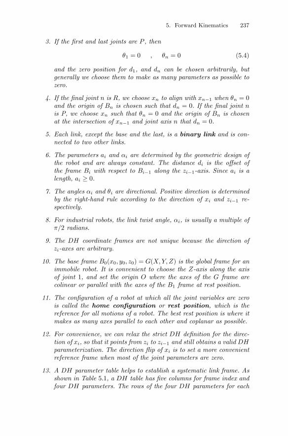
3. If the first and last joints are P , then
θ1 = 0 , θn = 0 (5.4)
and the zero position for d1, and dn can be chosen arbitrarily, butgenerally we choose them to make as many parameters as possible tozero.
4. If the final joint n is R, we choose xn to align with xn−1 when θn = 0and the origin of Bn is chosen such that dn = 0. If the final joint nis P, we choose xn such that θn = 0 and the origin of Bn is chosenat the intersection of xn−1 and joint axis n that dn = 0.
5. Each link, except the base and the last, is a binary link and is con-nected to two other links.
6. The parameters ai and αi are determined by the geometric design ofthe robot and are always constant. The distance di is the offset ofthe frame Bi with respect to Bi−1 along the zi−1-axis. Since ai is alength, ai ≥ 0.
7. The angles αi and θi are directional. Positive direction is determinedby the right-hand rule according to the direction of xi and zi−1 re-spectively.
8. For industrial robots, the link twist angle, αi, is usually a multiple ofπ/2 radians.
9. The DH coordinate frames are not unique because the direction ofzi-axes are arbitrary.
10. The base frame B0(x0, y0, z0) = G(X,Y,Z) is the global frame for animmobile robot. It is convenient to choose the Z-axis along the axisof joint 1, and set the origin O where the axes of the G frame arecolinear or parallel with the axes of the B1 frame at rest position.
11. The configuration of a robot at which all the joint variables are zerois called the home configuration or rest position, which is thereference for all motions of a robot. The best rest position is where itmakes as many axes parallel to each other and coplanar as possible.
12. For convenience, we can relax the strict DH definition for the direc-tion of xi, so that it points from zi to zi−1 and still obtains a valid DHparameterization. The direction flip of xi is to set a more convenientreference frame when most of the joint parameters are zero.
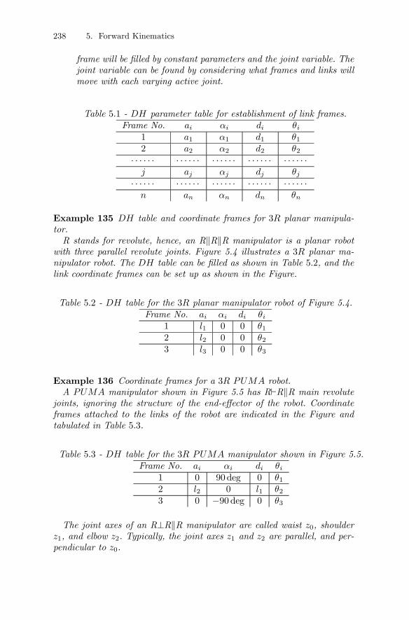
13. A DH parameter table helps to establish a systematic link frame. Asshown in Table 5.1, a DH table has five columns for frame index andfour DH parameters. The rows of the four DH parameters for each
238 5. Forward Kinematics
frame will be filled by constant parameters and the joint variable. Thejoint variable can be found by considering what frames and links willmove with each varying active joint.
Table 5.1 - DH parameter table for establishment of link frames.Frame No. ai αi di θi
1 a1 α1 d1 θ12 a2 α2 d2 θ2
· · · · · · · · · · · · · · · · · · · · · · · · · · · · · ·j aj αj dj θj
· · · · · · · · · · · · · · · · · · · · · · · · · · · · · ·n an αn dn θn
Example 135 DH table and coordinate frames for 3R planar manipula-tor.R stands for revolute, hence, an RkRkR manipulator is a planar robot
with three parallel revolute joints. Figure 5.4 illustrates a 3R planar ma-nipulator robot. The DH table can be filled as shown in Table 5.2, and thelink coordinate frames can be set up as shown in the Figure.
Table 5.2 - DH table for the 3R planar manipulator robot of Figure 5.4.Frame No. ai αi di θi
1 l1 0 0 θ12 l2 0 0 θ23 l3 0 0 θ3
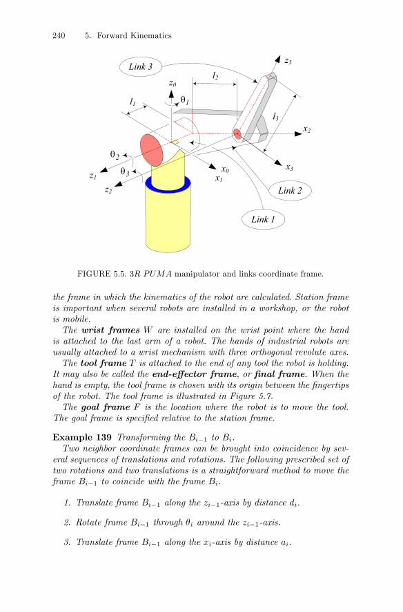
Example 136 Coordinate frames for a 3R PUMA robot.A PUMA manipulator shown in Figure 5.5 has R`RkR main revolute
joints, ignoring the structure of the end-effector of the robot. Coordinateframes attached to the links of the robot are indicated in the Figure andtabulated in Table 5.3.
Table 5.3 - DH table for the 3R PUMA manipulator shown in Figure 5.5.Frame No. ai αi di θi
1 0 90 deg 0 θ12 l2 0 l1 θ23 0 −90 deg 0 θ3
The joint axes of an R⊥RkR manipulator are called waist z0, shoulderz1, and elbow z2. Typically, the joint axes z1 and z2 are parallel, and per-pendicular to z0.
5. Forward Kinematics 239
l 3
x2y2
x3
y0
x0
z2
z3y0
y1
l1
l 2
x1
y3
z0x0
z1
1θ
2θ
3θ
B0
B1
B2
B3
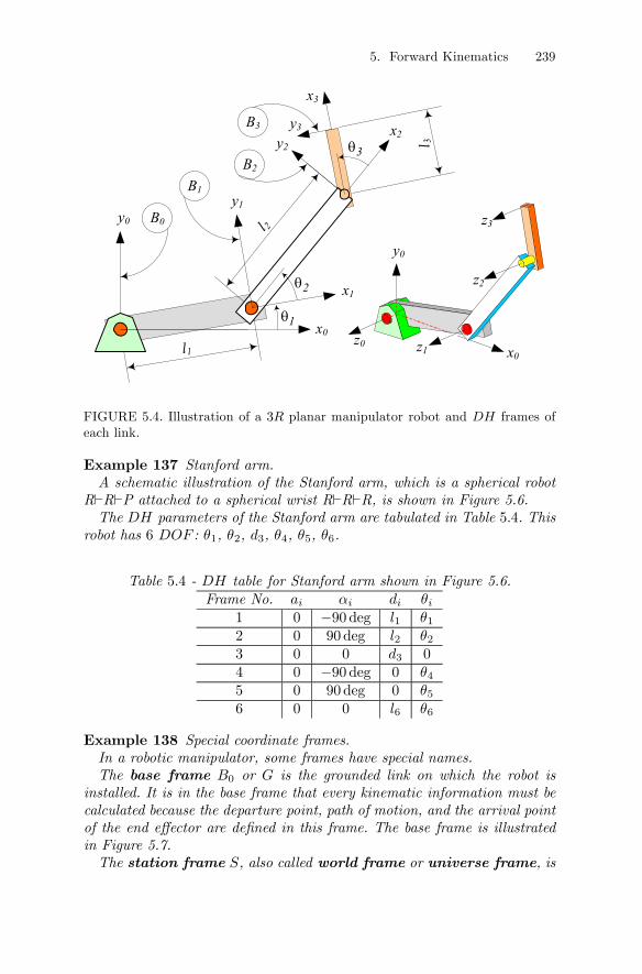
FIGURE 5.4. Illustration of a 3R planar manipulator robot and DH frames ofeach link.
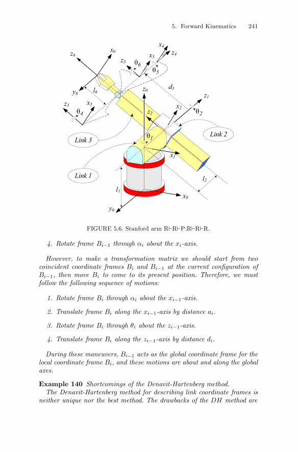
Example 137 Stanford arm.A schematic illustration of the Stanford arm, which is a spherical robot
R`R`P attached to a spherical wrist R`R`R, is shown in Figure 5.6.The DH parameters of the Stanford arm are tabulated in Table 5.4. This
robot has 6 DOF : θ1, θ2, d3, θ4, θ5, θ6.
Table 5.4 - DH table for Stanford arm shown in Figure 5.6.Frame No. ai αi di θi
1 0 −90 deg l1 θ12 0 90 deg l2 θ23 0 0 d3 04 0 −90 deg 0 θ45 0 90 deg 0 θ56 0 0 l6 θ6
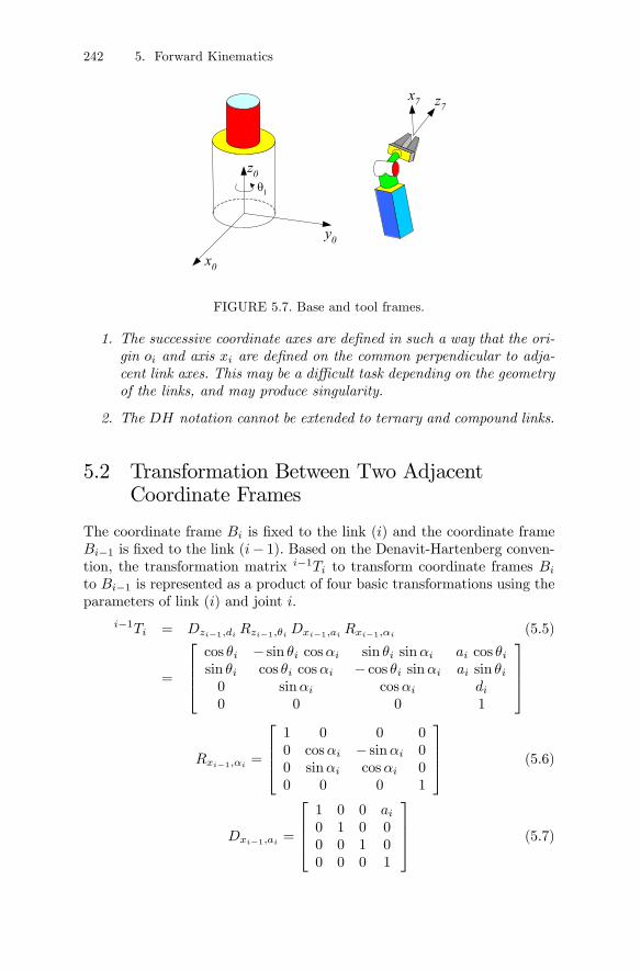
Example 138 Special coordinate frames.In a robotic manipulator, some frames have special names.The base frame B0 or G is the grounded link on which the robot is
installed. It is in the base frame that every kinematic information must becalculated because the departure point, path of motion, and the arrival pointof the end effector are defined in this frame. The base frame is illustratedin Figure 5.7.The station frame S, also called world frame or universe frame, is
240 5. Forward Kinematics
x1z1
x2
z2
z3
x3
z0l2
l3
x0
l1
Link 1
Link 2
Link 3
2θ
3θ
1θ
FIGURE 5.5. 3R PUMA manipulator and links coordinate frame.
the frame in which the kinematics of the robot are calculated. Station frameis important when several robots are installed in a workshop, or the robotis mobile.The wrist frames W are installed on the wrist point where the hand
is attached to the last arm of a robot. The hands of industrial robots areusually attached to a wrist mechanism with three orthogonal revolute axes.The tool frame T is attached to the end of any tool the robot is holding.
It may also be called the end-effector frame, or final frame. When thehand is empty, the tool frame is chosen with its origin between the fingertipsof the robot. The tool frame is illustrated in Figure 5.7.The goal frame F is the location where the robot is to move the tool.
The goal frame is specified relative to the station frame.
Example 139 Transforming the Bi−1 to Bi.Two neighbor coordinate frames can be brought into coincidence by sev-
eral sequences of translations and rotations. The following prescribed set oftwo rotations and two translations is a straightforward method to move theframe Bi−1 to coincide with the frame Bi.
1. Translate frame Bi−1 along the zi−1-axis by distance di.
2. Rotate frame Bi−1 through θi around the zi−1-axis.
3. Translate frame Bi−1 along the xi-axis by distance ai.
5. Forward Kinematics 241
l1
z2
d3
z3
z4z5
z6
x2
x0
x3
x4
x5
z0
y0
l6
l2
y6
x6
z1
x1
Link 1
Link 2Link 3
6θ
1θ
2θ4θ
5θ
z0
FIGURE 5.6. Stanford arm R`R`P:R`R`R.
4. Rotate frame Bi−1 through αi about the xi-axis.
However, to make a transformation matrix we should start from twocoincident coordinate frames Bi and Bi−1 at the current configuration ofBi−1, then move Bi to come to its present position. Therefore, we mustfollow the following sequence of motions:
1. Rotate frame Bi through αi about the xi−1-axis.
2. Translate frame Bi along the xi−1-axis by distance ai.
3. Rotate frame Bi through θi about the zi−1-axis.
4. Translate frame Bi along the zi−1-axis by distance di.
During these maneuvers, Bi−1 acts as the global coordinate frame for thelocal coordinate frame Bi, and these motions are about and along the globalaxes.
Example 140 Shortcomings of the Denavit-Hartenberg method.The Denavit-Hartenberg method for describing link coordinate frames is
neither unique nor the best method. The drawbacks of the DH method are
242 5. Forward Kinematics
θ1
z0
z7
x0
x7
y0
FIGURE 5.7. Base and tool frames.
1. The successive coordinate axes are defined in such a way that the ori-gin oi and axis xi are defined on the common perpendicular to adja-cent link axes. This may be a difficult task depending on the geometryof the links, and may produce singularity.
2. The DH notation cannot be extended to ternary and compound links.
5.2 Transformation Between Two AdjacentCoordinate Frames
The coordinate frame Bi is fixed to the link (i) and the coordinate frameBi−1 is fixed to the link (i− 1). Based on the Denavit-Hartenberg conven-tion, the transformation matrix i−1Ti to transform coordinate frames Bi
to Bi−1 is represented as a product of four basic transformations using theparameters of link (i) and joint i.
i−1Ti = Dzi−1,di Rzi−1,θi Dxi−1,ai Rxi−1,αi (5.5)
=
⎡⎢⎢⎣cos θi − sin θi cosαi sin θi sinαi ai cos θisin θi cos θi cosαi − cos θi sinαi ai sin θi0 sinαi cosαi di0 0 0 1
⎤⎥⎥⎦
Rxi−1,αi =
⎡⎢⎢⎣1 0 0 00 cosαi − sinαi 00 sinαi cosαi 00 0 0 1
⎤⎥⎥⎦ (5.6)
Dxi−1,ai =
⎡⎢⎢⎣1 0 0 ai0 1 0 00 0 1 00 0 0 1
⎤⎥⎥⎦ (5.7)
5. Forward Kinematics 243
Rzi−1,θi =
⎡⎢⎢⎣cos θi − sin θi 0 0sin θi cos θi 0 00 0 1 00 0 0 1
⎤⎥⎥⎦ (5.8)
Dzi−1,di =
⎡⎢⎢⎣1 0 0 00 1 0 00 0 1 di0 0 0 1
⎤⎥⎥⎦ . (5.9)
Therefore the transformation equation from coordinate frame Bi(xi, yi,zi), to its previous coordinate frame Bi−1(xi−1, yi−1, zi−1), is⎡⎢⎢⎣
xi−1yi−1zi−11
⎤⎥⎥⎦ = i−1Ti
⎡⎢⎢⎣xiyizi1
⎤⎥⎥⎦ (5.10)
where,
i−1Ti =
⎡⎢⎢⎣cos θi − sin θi cosαi sin θi sinαi ai cos θisin θi cos θi cosαi − cos θi sinαi ai sin θi0 sinαi cosαi di0 0 0 1
⎤⎥⎥⎦ . (5.11)
This 4×4 matrix may be partitioned into two submatrices, which representa unique rotation combined with a unique translation to produce the samerigid motion required to move from Bi to Bi−1,
i−1Ti =
∙i−1Ri
i−1di0 1
¸(5.12)
where
i−1Ri =
⎡⎣ cos θi − sin θi cosαi sin θi sinαisin θi cos θi cosαi − cos θi sinαi0 sinαi cosαi
⎤⎦ (5.13)
and
i−1di =
⎡⎣ ai cos θiai sin θi
di
⎤⎦ . (5.14)
The inverse of the homogeneous transformation matrix (5.11) is
iTi−1 = i−1T−1i (5.15)
=
⎡⎢⎢⎣cos θi sin θi 0 −ai
− sin θi cosαi cos θi cosαi sinαi −di sinαisin θi sinαi − cos θi sinαi cosαi −di cosαi
0 0 0 1
⎤⎥⎥⎦ .
244 5. Forward Kinematics
x1
y1
z1
rP
x2
y2
z2
o1
o2
P
s2
a2
d2
2
2θ
2α
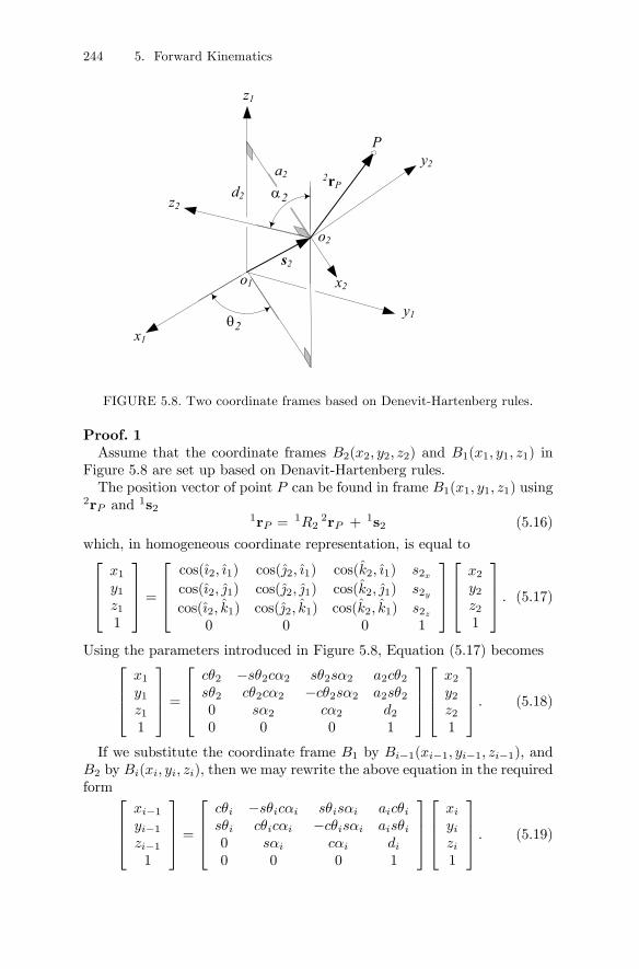
FIGURE 5.8. Two coordinate frames based on Denevit-Hartenberg rules.
Proof. 1Assume that the coordinate frames B2(x2, y2, z2) and B1(x1, y1, z1) in
Figure 5.8 are set up based on Denavit-Hartenberg rules.The position vector of point P can be found in frame B1(x1, y1, z1) using
2rP and 1s21rP =
1R22rP +
1s2 (5.16)
which, in homogeneous coordinate representation, is equal to⎡⎢⎢⎣x1y1z11
⎤⎥⎥⎦ =⎡⎢⎢⎣cos(ı2, ı1) cos(j2, ı1) cos(k2, ı1) s2xcos(ı2, j1) cos(j2, j1) cos(k2, j1) s2ycos(ı2, k1) cos(j2, k1) cos(k2, k1) s2z
0 0 0 1
⎤⎥⎥⎦⎡⎢⎢⎣
x2y2z21
⎤⎥⎥⎦ . (5.17)Using the parameters introduced in Figure 5.8, Equation (5.17) becomes⎡⎢⎢⎣
x1y1z11
⎤⎥⎥⎦ =⎡⎢⎢⎣
cθ2 −sθ2cα2 sθ2sα2 a2cθ2sθ2 cθ2cα2 −cθ2sα2 a2sθ20 sα2 cα2 d20 0 0 1
⎤⎥⎥⎦⎡⎢⎢⎣
x2y2z21
⎤⎥⎥⎦ . (5.18)
If we substitute the coordinate frame B1 by Bi−1(xi−1, yi−1, zi−1), andB2 by Bi(xi, yi, zi), then we may rewrite the above equation in the requiredform ⎡⎢⎢⎣
xi−1yi−1zi−11
⎤⎥⎥⎦ =⎡⎢⎢⎣
cθi −sθicαi sθisαi aicθisθi cθicαi −cθisαi aisθi0 sαi cαi di0 0 0 1
⎤⎥⎥⎦⎡⎢⎢⎣
xiyizi1
⎤⎥⎥⎦ . (5.19)
5. Forward Kinematics 245
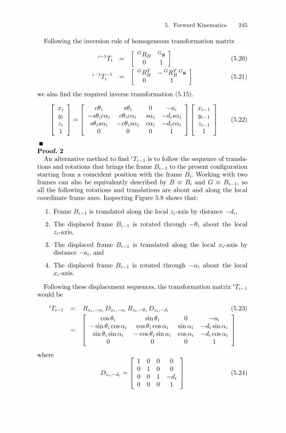
Following the inversion rule of homogeneous transformation matrix
i−1Ti =
∙GRB
Gs0 1
¸(5.20)
i−1T−1i =
∙GRT
B −GRTBGs
0 1
¸(5.21)
we also find the required inverse transformation (5.15).⎡⎢⎢⎣xiyizi1
⎤⎥⎥⎦ =⎡⎢⎢⎣
cθi sθi 0 −ai−sθicαi cθicαi sαi −disαisθisαi −cθisαi cαi −dicαi0 0 0 1
⎤⎥⎥⎦⎡⎢⎢⎣
xi−1yi−1zi−11
⎤⎥⎥⎦ (5.22)
Proof. 2An alternative method to find iTi−1 is to follow the sequence of transla-
tions and rotations that brings the frame Bi−1 to the present configurationstarting from a coincident position with the frame Bi. Working with twoframes can also be equivalently described by B ≡ Bi and G ≡ Bi−1, soall the following rotations and translations are about and along the localcoordinate frame axes. Inspecting Figure 5.8 shows that:
1. Frame Bi−1 is translated along the local zi-axis by distance −di,
2. The displaced frame Bi−1 is rotated through −θi about the localzi-axis,
3. The displaced frame Bi−1 is translated along the local xi-axis bydistance −ai, and
4. The displaced frame Bi−1 is rotated through −αi about the localxi-axis.
Following these displacement sequences, the transformation matrix iTi−1would be
iTi−1 = Rxi,−αi Dxi,−ai Rzi,−θi Dzi,−di (5.23)
=
⎡⎢⎢⎣cos θi sin θi 0 −ai
− sin θi cosαi cos θi cosαi sinαi −di sinαisin θi sinαi − cos θi sinαi cosαi −di cosαi
0 0 0 1
⎤⎥⎥⎦where
Dzi,−di =
⎡⎢⎢⎣1 0 0 00 1 0 00 0 1 −di0 0 0 1
⎤⎥⎥⎦ (5.24)
246 5. Forward Kinematics
x2y2
y0
y1
l1
l 2
x1
x0
2θ
1θ
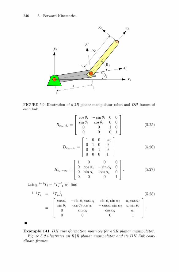
FIGURE 5.9. Illustration of a 2R planar manipulator robot and DH frames ofeach link.
Rzi,−θi =
⎡⎢⎢⎣cos θi − sin θi 0 0sin θi cos θi 0 00 0 1 00 0 0 1
⎤⎥⎥⎦ (5.25)
Dxi,−ai =
⎡⎢⎢⎣1 0 0 −ai0 1 0 00 0 1 00 0 0 1
⎤⎥⎥⎦ (5.26)
Rxi,−αi =
⎡⎢⎢⎣1 0 0 00 cosαi − sinαi 00 sinαi cosαi 00 0 0 1
⎤⎥⎥⎦ . (5.27)
Using i−1Ti =iT−1i−1 we find
i−1Ti = iT−1i−1 (5.28)
=
⎡⎢⎢⎣cos θi − sin θi cosαi sin θi sinαi ai cos θisin θi cos θi cosαi − cos θi sinαi ai sin θi0 sinαi cosαi di0 0 0 1
⎤⎥⎥⎦ .
Example 141 DH transformation matrices for a 2R planar manipulator.Figure 5.9 illustrates an RkR planar manipulator and its DH link coor-
dinate frames.
5. Forward Kinematics 247
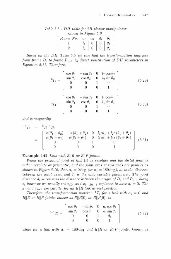
Table 5.5 - DH table for 2R planar manipulatorshown in Figure 5.9.
Frame No. ai αi di θi1 l1 0 0 θ12 l2 0 0 θ2
Based on the DH Table 5.5 we can find the transformation matricesfrom frame Bi to frame Bi−1 by direct substitution of DH parameters inEquation 5.11. Therefore,
1T2 =
⎡⎢⎢⎣cos θ2 − sin θ2 0 l2 cos θ2sin θ2 cos θ2 0 l2 sin θ20 0 1 00 0 0 1
⎤⎥⎥⎦ (5.29)
0T1 =
⎡⎢⎢⎣cos θ1 − sin θ1 0 l1 cos θ1sin θ1 cos θ1 0 l1 sin θ10 0 1 00 0 0 1
⎤⎥⎥⎦ (5.30)
and consequently
0T2 = 0T11T2
=
⎡⎢⎢⎣c (θ1 + θ2) −s (θ1 + θ2) 0 l1cθ1 + l2c (θ1 + θ2)s (θ1 + θ2) c (θ1 + θ2) 0 l1sθ1 + l2s (θ1 + θ2)
0 0 1 00 0 0 1
⎤⎥⎥⎦ . (5.31)Example 142 Link with RkR or RkP joints.When the proximal joint of link (i) is revolute and the distal joint is
either revolute or prismatic, and the joint axes at two ends are parallel asshown in Figure 5.10, then αi = 0deg (or αi = 180 deg), ai is the distancebetween the joint axes, and θi is the only variable parameter. The jointdistance di = const is the distance between the origin of Bi and Bi−1 alongzi however we usually set xiyi and xi−1yi−1 coplanar to have di = 0. Thexi and xi−1 are parallel for an RkR link at rest position.Therefore, the transformation matrix i−1Ti for a link with αi = 0 and
RkR or RkP joints, known as RkR(0) or RkP(0), is
i−1Ti =
⎡⎢⎢⎣cos θi − sin θi 0 ai cos θisin θi cos θi 0 ai sin θi0 0 1 di0 0 0 1
⎤⎥⎥⎦ (5.32)
while for a link with αi = 180deg and RkR or RkP joints, known as
248 5. Forward Kinematics
iθ
yi-1
yixi
zi-1
xi-1
zi
xi
xi-1
a i
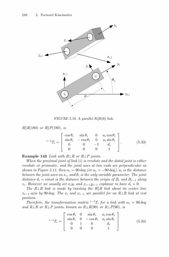
FIGURE 5.10. A parallel RkR(0) link.
RkR(180) or RkP(180), is
i−1Ti =
⎡⎢⎢⎣cos θi sin θi 0 ai cos θisin θi − cos θi 0 ai sin θi0 0 −1 di0 0 0 1
⎤⎥⎥⎦ . (5.33)
Example 143 Link with R⊥R or R⊥P joints.When the proximal joint of link (i) is revolute and the distal joint is either
revolute or prismatic, and the joint axes at two ends are perpendicular asshown in Figure 5.11, then αi = 90deg (or αi = −90 deg), ai is the distancebetween the joint axes on xi, and θi is the only variable parameter. The jointdistance di = const is the distance between the origin of Bi and Bi−1 alongzi. However we usually set xiyi and xi−1yi−1 coplanar to have di = 0.The R⊥R link is made by twisting the RkR link about its center line
xi−1-axis by 90 deg. The xi and xi−1 are parallel for an R⊥R link at restposition.Therefore, the transformation matrix i−1Ti for a link with αi = 90deg
and R⊥R or R⊥P joints, known as R⊥R(90) or R⊥P(90), is
i−1Ti =
⎡⎢⎢⎣cos θi 0 sin θi ai cos θisin θi 0 − cos θi ai sin θi0 1 0 di0 0 0 1
⎤⎥⎥⎦ (5.34)
5. Forward Kinematics 249
iθ
yi-1
xi
zi-1
xi-1
zi
xi
xi-1
ziai
FIGURE 5.11. A perpendicular R⊥R(90) link.
while for a link with αi = −90 deg and R⊥R or R⊥P joints, known asR⊥R(−90) or R⊥P(−90), is
i−1Ti =
⎡⎢⎢⎣cos θi 0 − sin θi ai cos θisin θi 0 cos θi ai sin θi0 −1 0 di0 0 0 1
⎤⎥⎥⎦ . (5.35)
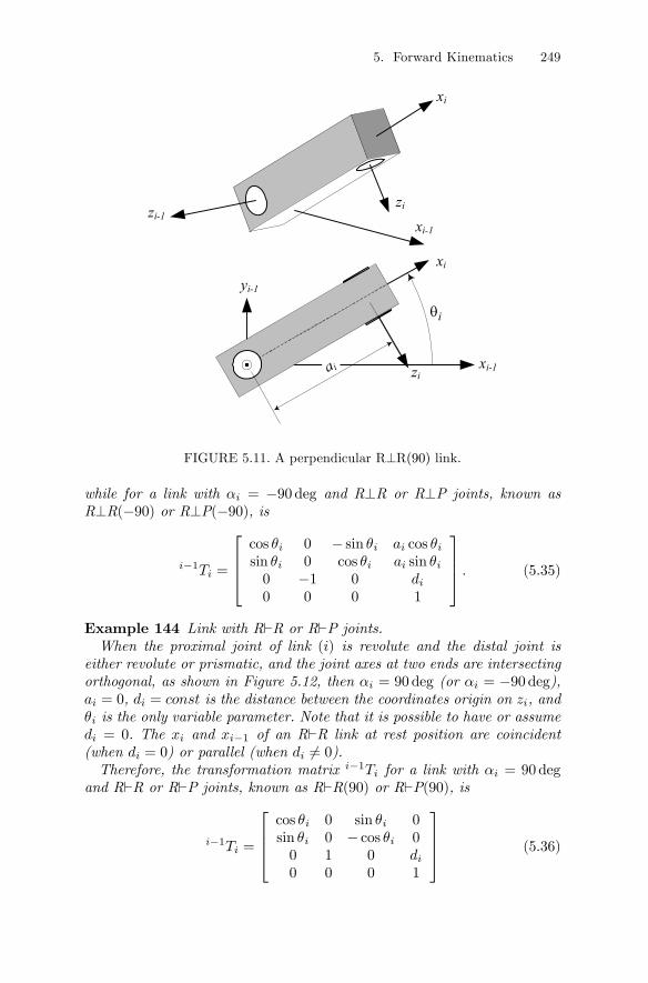
Example 144 Link with R`R or R`P joints.When the proximal joint of link (i) is revolute and the distal joint is
either revolute or prismatic, and the joint axes at two ends are intersectingorthogonal, as shown in Figure 5.12, then αi = 90deg (or αi = −90 deg),ai = 0, di = const is the distance between the coordinates origin on zi, andθi is the only variable parameter. Note that it is possible to have or assumedi = 0. The xi and xi−1 of an R`R link at rest position are coincident(when di = 0) or parallel (when di 6= 0).Therefore, the transformation matrix i−1Ti for a link with αi = 90deg
and R`R or R`P joints, known as R`R(90) or R`P(90), is
i−1Ti =
⎡⎢⎢⎣cos θi 0 sin θi 0sin θi 0 − cos θi 00 1 0 di0 0 0 1
⎤⎥⎥⎦ (5.36)
250 5. Forward Kinematics
iθ
yi-1
zi-1
xi-1
zixi-1
zi
xi
xi
iθ
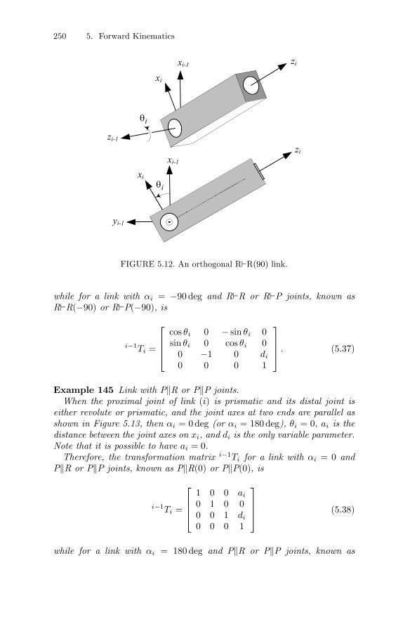
FIGURE 5.12. An orthogonal R`R(90) link.
while for a link with αi = −90 deg and R`R or R`P joints, known asR`R(−90) or R`P(−90), is
i−1Ti =
⎡⎢⎢⎣cos θi 0 − sin θi 0sin θi 0 cos θi 00 −1 0 di0 0 0 1
⎤⎥⎥⎦ . (5.37)
Example 145 Link with PkR or PkP joints.When the proximal joint of link (i) is prismatic and its distal joint is
either revolute or prismatic, and the joint axes at two ends are parallel asshown in Figure 5.13, then αi = 0deg (or αi = 180deg), θi = 0, ai is thedistance between the joint axes on xi, and di is the only variable parameter.Note that it is possible to have ai = 0.Therefore, the transformation matrix i−1Ti for a link with αi = 0 and
PkR or PkP joints, known as PkR(0) or PkP(0), is
i−1Ti =
⎡⎢⎢⎣1 0 0 ai0 1 0 00 0 1 di0 0 0 1
⎤⎥⎥⎦ (5.38)
while for a link with αi = 180 deg and PkR or PkP joints, known as
5. Forward Kinematics 251
yi-1
yi
ai
xizi-1
xi-1
zi
xixi-1
di
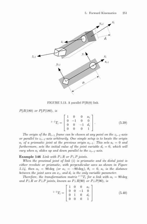
FIGURE 5.13. A parallel PkR(0) link.
PkR(180) or PkP(180), is
i−1Ti =
⎡⎢⎢⎣1 0 0 ai0 −1 0 00 0 −1 di0 0 0 1
⎤⎥⎥⎦ . (5.39)
The origin of the Bi−1 frame can be chosen at any point on the zi−1-axisor parallel to zi−1-axis arbitrarily. One simple setup is to locate the originoi of a prismatic joint at the previous origin oi−1. This sets ai = 0 andfurthermore, sets the initial value of the joint variable di = 0, which willvary when oi slides up and down parallel to the zi−1-axis.
Example 146 Link with P⊥R or P⊥P joints.When the proximal joint of link (i) is prismatic and its distal joint is
either revolute or prismatic, with perpendicular axes as shown in Figure5.14, then αi = 90deg (or αi = −90 deg), θi = 0, ai is the distancebetween the joint axes on xi, and di is the only variable parameter.Therefore, the transformation matrix i−1Ti for a link with αi = 90deg
and P⊥R or P⊥P joints, known as P⊥R(90) or P⊥P(90), is
i−1Ti =
⎡⎢⎢⎣1 0 0 ai0 0 −1 00 1 0 di0 0 0 1
⎤⎥⎥⎦ (5.40)
252 5. Forward Kinematics
zi-1
xi
zi-1
xi-1
zi
xi
xi-1
yi
di
di
ai
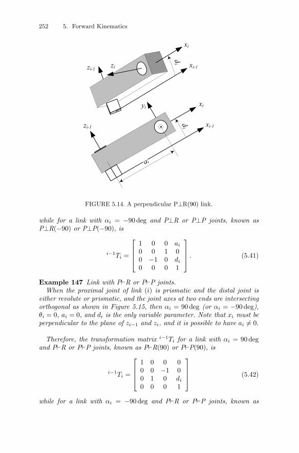
FIGURE 5.14. A perpendicular P⊥R(90) link.
while for a link with αi = −90 deg and P⊥R or P⊥P joints, known asP⊥R(−90) or P⊥P(−90), is
i−1Ti =
⎡⎢⎢⎣1 0 0 ai0 0 1 00 −1 0 di0 0 0 1
⎤⎥⎥⎦ . (5.41)
Example 147 Link with P`R or P`P joints.When the proximal joint of link (i) is prismatic and the distal joint is
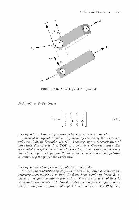
either revolute or prismatic, and the joint axes at two ends are intersectingorthogonal as shown in Figure 5.15, then αi = 90deg (or αi = −90 deg),θi = 0, ai = 0, and di is the only variable parameter. Note that xi must beperpendicular to the plane of zi−1 and zi, and it is possible to have ai 6= 0.
Therefore, the transformation matrix i−1Ti for a link with αi = 90degand P`R or P`P joints, known as P`R(90) or P`P(90), is
i−1Ti =
⎡⎢⎢⎣1 0 0 00 0 −1 00 1 0 di0 0 0 1
⎤⎥⎥⎦ (5.42)
while for a link with αi = −90 deg and P`R or P`P joints, known as
5. Forward Kinematics 253
yi-1
zi-1
xi-1zixi
xi-1
zi
xi
di
FIGURE 5.15. An orthogonal P`R(90) link.
P`R(−90) or P`P(−90), is
i−1Ti =
⎡⎢⎢⎣1 0 0 00 0 1 00 −1 0 di0 0 0 1
⎤⎥⎥⎦ . (5.43)
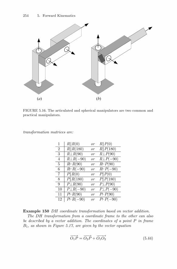
Example 148 Assembling industrial links to make a manipulator.Industrial manipulators are usually made by connecting the introduced
industrial links in Examples 142-147. A manipulator is a combination ofthree links that provide three DOF to a point in a Cartesian space. Thearticulated and spherical manipulators are two common and practical ma-nipulators. Figure 5.16(a) and (b) show how we make these manipulatorsby connecting the proper industrial links.
Example 149 Classification of industrial robot links.A robot link is identified by its joints at both ends, which determines the
transformation matrix to go from the distal joint coordinate frame Bi tothe proximal joint coordinate frame Bi−1. There are 12 types of links tomake an industrial robot. The transformation matrix for each type dependssolely on the proximal joint, and angle between the z-axes. The 12 types of
254 5. Forward Kinematics
(a) (b)
FIGURE 5.16. The articulated and spherical manipulators are two common andpractical manipulators.
transformation matrices are:
1 RkR(0) or RkP(0)2 RkR(180) or RkP(180)3 R⊥R(90) or R⊥P(90)4 R⊥R(−90) or R⊥P(−90)5 R`R(90) or R`P(90)6 R`R(−90) or R`P(−90)7 PkR(0) or PkP(0)8 PkR(180) or PkP(180)9 P⊥R(90) or P⊥P(90)10 P⊥R(−90) or P⊥P(−90)11 P`R(90) or P`P(90)12 P`R(−90) or P`P(−90)
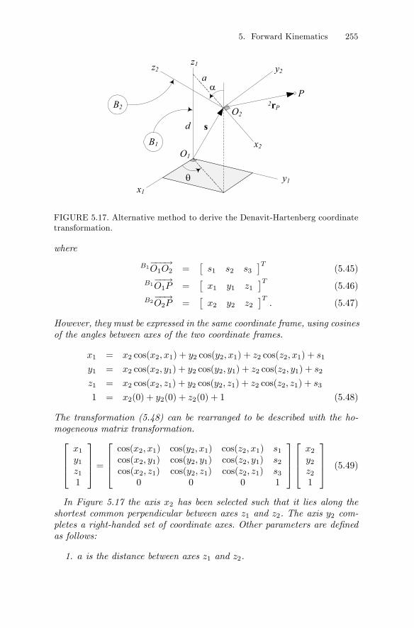
Example 150 DH coordinate transformation based on vector addition.The DH transformation from a coordinate frame to the other can also
be described by a vector addition. The coordinates of a point P in frameB1, as shown in Figure 5.17, are given by the vector equation
−−→O1P =
−−→O2P +
−−−→O1O2 (5.44)
5. Forward Kinematics 255
x1
s
PB2
B1
y1
z1
x2
y2z2
O2
O1
d
a
θ
rP2
α
FIGURE 5.17. Alternative method to derive the Denavit-Hartenberg coordinatetransformation.
where
B1−−−→O1O2 =
£s1 s2 s3
¤T(5.45)
B1−−→O1P =
£x1 y1 z1
¤T(5.46)
B2−−→O2P =
£x2 y2 z2
¤T. (5.47)
However, they must be expressed in the same coordinate frame, using cosinesof the angles between axes of the two coordinate frames.
x1 = x2 cos(x2, x1) + y2 cos(y2, x1) + z2 cos(z2, x1) + s1
y1 = x2 cos(x2, y1) + y2 cos(y2, y1) + z2 cos(z2, y1) + s2
z1 = x2 cos(x2, z1) + y2 cos(y2, z1) + z2 cos(z2, z1) + s3
1 = x2(0) + y2(0) + z2(0) + 1 (5.48)
The transformation (5.48) can be rearranged to be described with the ho-mogeneous matrix transformation.⎡⎢⎢⎣
x1y1z11
⎤⎥⎥⎦ =⎡⎢⎢⎣cos(x2, x1) cos(y2, x1) cos(z2, x1) s1cos(x2, y1) cos(y2, y1) cos(z2, y1) s2cos(x2, z1) cos(y2, z1) cos(z2, z1) s3
0 0 0 1
⎤⎥⎥⎦⎡⎢⎢⎣
x2y2z21
⎤⎥⎥⎦ (5.49)
In Figure 5.17 the axis x2 has been selected such that it lies along theshortest common perpendicular between axes z1 and z2. The axis y2 com-pletes a right-handed set of coordinate axes. Other parameters are definedas follows:
1. a is the distance between axes z1 and z2.
256 5. Forward Kinematics
2. α is the twist angle that screws the z1-axis into the z2-axis along a.
3. d is the distance from the x1-axis to the x2-axis.
4. θ is the angle that screws the x1-axis into the x2-axis along d.
Using these definitions, the homogeneous transformation matrix becomes,⎡⎢⎢⎣x1y1z11
⎤⎥⎥⎦ =⎡⎢⎢⎣cos θ − sin θ cosα − sin θ sinα a cos θsin θ cos θ cosα cos θ sinα a sin θ0 − sinα cosα d0 0 0 1
⎤⎥⎥⎦⎡⎢⎢⎣
x2y2z21
⎤⎥⎥⎦ (5.50)
or1rP =
1T22rP (5.51)
where1T2 = (a, α, d, θ). (5.52)
The parameters a, α, θ, d define the configuration of B2 with respect to B1and belong to B2. Hence, in general, the parameters ai, αi, θi, di define theconfiguration of Bi with respect to Bi−1 and belong to Bi.
i−1Ti = (ai, αi, di, θi). (5.53)
Example 151 The same DH transformation matrix.Because in DH method of setting coordinate frames, a translation D and
a rotation R are about and along one axis, it is immaterial if we apply thetranslation D first and then the rotation R or vice versa. Therefore, we canchange the order of D and R about and along the same axis and obtain thesame DH transformation matrix 5.11. Therefore,
i−1Ti = Dzi,di Rzi,θi Dxi,ai Rxi,αi
= Rzi,θi Dzi,di Dxi,ai Rxi,αi
= Dzi,di Rzi,θi Rxi,αi Dxi,ai
= Rzi,θi Dzi,di Rxi,αi Dxi,ai . (5.54)
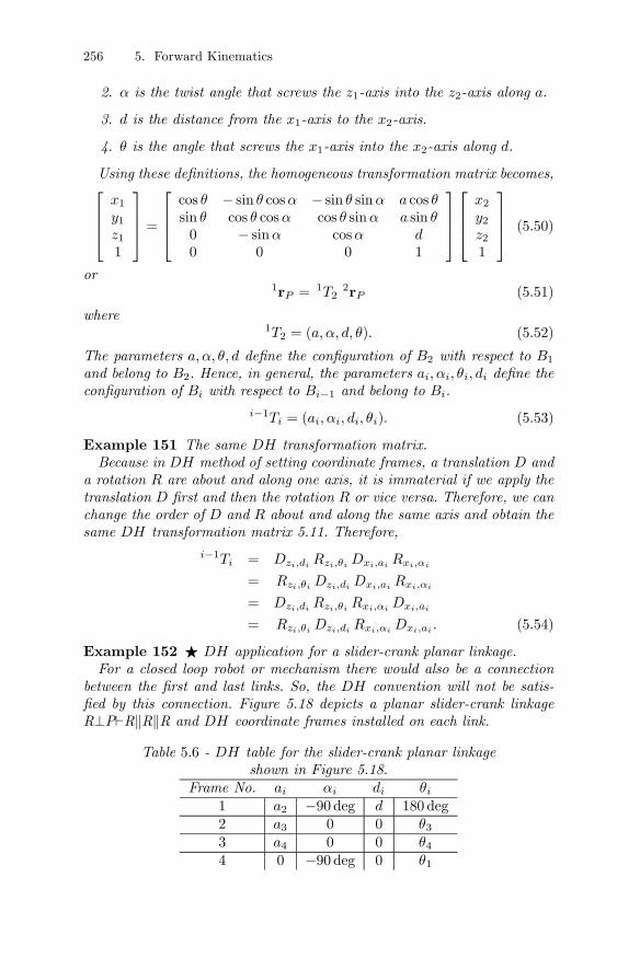
Example 152 F DH application for a slider-crank planar linkage.For a closed loop robot or mechanism there would also be a connection
between the first and last links. So, the DH convention will not be satis-fied by this connection. Figure 5.18 depicts a planar slider-crank linkageR⊥P`RkRkR and DH coordinate frames installed on each link.
Table 5.6 - DH table for the slider-crank planar linkageshown in Figure 5.18.
Frame No. ai αi di θi1 a2 −90 deg d 180 deg2 a3 0 0 θ33 a4 0 0 θ44 0 −90 deg 0 θ1
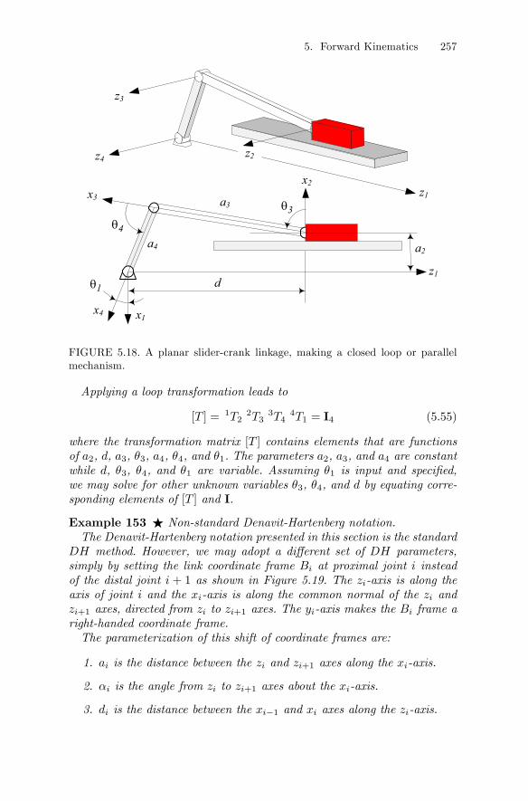
5. Forward Kinematics 257
x3
z1
x1
a4
x4
a3
x2
a2
d
z1
z2
z3
z4
1θ
4θ3θ
FIGURE 5.18. A planar slider-crank linkage, making a closed loop or parallelmechanism.
Applying a loop transformation leads to
[T ] = 1T22T3
3T44T1 = I4 (5.55)
where the transformation matrix [T ] contains elements that are functionsof a2, d, a3, θ3, a4, θ4, and θ1. The parameters a2, a3, and a4 are constantwhile d, θ3, θ4, and θ1 are variable. Assuming θ1 is input and specified,we may solve for other unknown variables θ3, θ4, and d by equating corre-sponding elements of [T ] and I.
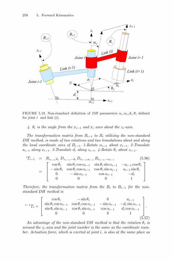
Example 153 F Non-standard Denavit-Hartenberg notation.The Denavit-Hartenberg notation presented in this section is the standard
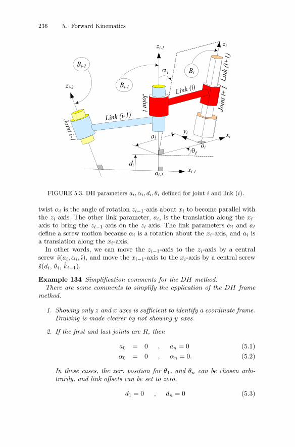
DH method. However, we may adopt a different set of DH parameters,simply by setting the link coordinate frame Bi at proximal joint i insteadof the distal joint i + 1 as shown in Figure 5.19. The zi-axis is along theaxis of joint i and the xi-axis is along the common normal of the zi andzi+1 axes, directed from zi to zi+1 axes. The yi-axis makes the Bi frame aright-handed coordinate frame.The parameterization of this shift of coordinate frames are:
1. ai is the distance between the zi and zi+1 axes along the xi-axis.
2. αi is the angle from zi to zi+1 axes about the xi-axis.
3. di is the distance between the xi−1 and xi axes along the zi-axis.
258 5. Forward Kinematics
iα
zi+1
Link (i)
Link (i+1)
Joint i-1
zi-1
xi-1
xiyi oi
oi-1
Bi
Bi-2Bi-1
Link (i-1)
Joint i Joint i+1
zi
ai
di
iθ
FIGURE 5.19. Non-standard definition of DH parameters ai, αi, di, θi definedfor joint i and link (i).
4. θi is the angle from the xi−1 and xi axes about the zi-axis.
The transformation matrix from Bi−1 to Bi utilizing the non-standardDH method, is made of two rotations and two translations about and alongthe local coordinate axes of Bi−1. 1-Rotate αi−1 about xi−1. 2-Translateai−1 along xi−1. 3-Translate di along zi−1. 4-Rotate θi about zi−1.
iTi−1 = Rzi−1,θi Dzi−1,−di Dxi−1,ai−1 Rxi−1,−αi−1 (5.56)
=
⎡⎢⎢⎣cos θi sin θi cosαi−1 sin θi sinαi−1 −ai−1 cos θi− sin θi cos θi cosαi−1 cos θi sinαi−1 ai−1 sin θi0 − sinαi−1 cosαi−1 −di0 0 0 1
⎤⎥⎥⎦Therefore, the transformation matrix from the Bi to Bi−1 for the non-standard DH method is
i−1Ti =
⎡⎢⎢⎣cos θi − sin θi 0 ai−1
sin θi cosαi−1 cos θi cosαi−1 − sinαi−1 −di sinαi−1sin θi sinαi−1 cos θi sinαi−1 cosαi−1 di cosαi−1
0 0 0 1
⎤⎥⎥⎦ .(5.57)
An advantage of the non-standard DH method is that the rotation θi isaround the zi-axis and the joint number is the same as the coordinate num-ber. Actuation force, which is exerted at joint i, is also at the same place as
5. Forward Kinematics 259
B0
O
0
P
rP znxn
x1
x0
z0
z1
z2
x2
y0
B1
B2
Bn
FIGURE 5.20. The position of the final frame in the base frame.
the coordinate frame Bi. Addressing the link’s geometrical characteristics,such as center of gravity, are more natural in this system.A disadvantage of the non-standard DH method is that the transforma-
tion matrix is a mix of i− 1 and i indices.Applying the standard or non-standard notation is a personal preference,
since both can be applied effectively.
5.3 Forward Position Kinematics of Robots
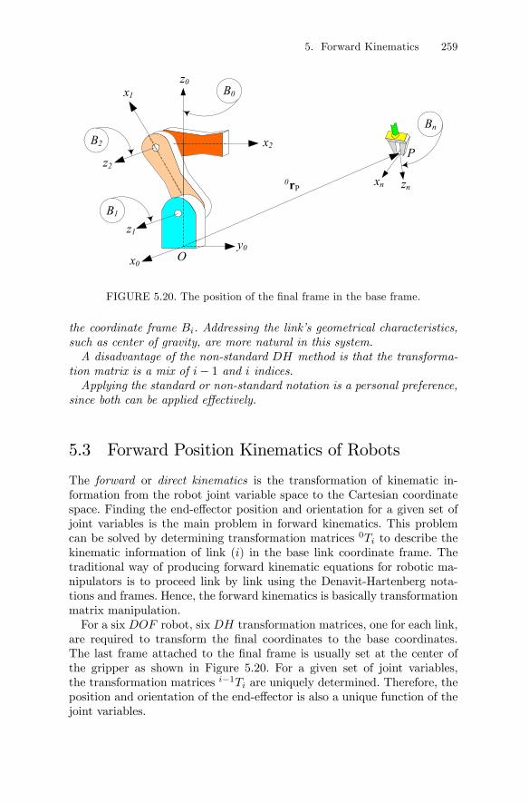
The forward or direct kinematics is the transformation of kinematic in-formation from the robot joint variable space to the Cartesian coordinatespace. Finding the end-effector position and orientation for a given set ofjoint variables is the main problem in forward kinematics. This problemcan be solved by determining transformation matrices 0Ti to describe thekinematic information of link (i) in the base link coordinate frame. Thetraditional way of producing forward kinematic equations for robotic ma-nipulators is to proceed link by link using the Denavit-Hartenberg nota-tions and frames. Hence, the forward kinematics is basically transformationmatrix manipulation.For a six DOF robot, six DH transformation matrices, one for each link,
are required to transform the final coordinates to the base coordinates.The last frame attached to the final frame is usually set at the center ofthe gripper as shown in Figure 5.20. For a given set of joint variables,the transformation matrices i−1Ti are uniquely determined. Therefore, theposition and orientation of the end-effector is also a unique function of thejoint variables.
260 5. Forward Kinematics
x2y2
x3y0
y1
l1
l 2
x1
y3
x0
l 3
X
Y
1θ
2θ
3θ ϕ
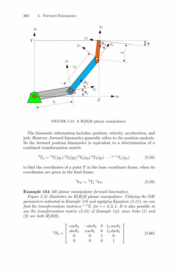
FIGURE 5.21. A RkRkR planar manipulator.
The kinematic information includes: position, velocity, acceleration, andjerk. However, forward kinematics generally refers to the position analysis.So the forward position kinematics is equivalent to a determination of acombined transformation matrix
0Tn =0T1(q1)
1T2(q2)2T3(q3)
3T4(q4) · · · n−1Tn(qn) (5.58)
to find the coordinates of a point P in the base coordinate frame, when itscoordinates are given in the final frame.
0rP =0Tn
nrP (5.59)
Example 154 3R planar manipulator forward kinematics.Figure 5.21 illustrates an RkRkR planar manipulator. Utilizing the DH
parameters indicated in Example 135 and applying Equation (5.11), we canfind the transformation matrices i−1Ti for i = 3, 2, 1. It is also possible touse the transformation matrix (5.32) of Example 142, since links (1) and(2) are both RkR(0).
2T3 =
⎡⎢⎢⎣cos θ3 − sin θ3 0 l3 cos θ3sin θ3 cos θ3 0 l3 sin θ30 0 1 00 0 0 1
⎤⎥⎥⎦ (5.60)
5. Forward Kinematics 261
1T2 =
⎡⎢⎢⎣cos θ2 − sin θ2 0 l2 cos θ2sin θ2 cos θ2 0 l2 sin θ20 0 1 00 0 0 1
⎤⎥⎥⎦ (5.61)
0T1 =
⎡⎢⎢⎣cos θ1 − sin θ1 0 l1 cos θ1sin θ1 cos θ1 0 l1 sin θ10 0 1 00 0 0 1
⎤⎥⎥⎦ (5.62)
Therefore, the transformation matrix to relate the end-effector frame to thebase frame is:
0T3 = 0T11T2
2T3
=
⎡⎢⎢⎣cos (θ1 + θ2 + θ3) − sin (θ1 + θ2 + θ3) 0 r14sin (θ1 + θ2 + θ3) cos (θ1 + θ2 + θ3) 0 r24
0 0 1 00 0 0 1
⎤⎥⎥⎦ (5.63)
r14 = l1 cos θ1 + l2 cos (θ1 + θ2) + l3 cos (θ1 + θ2 + θ3)
r24 = l1 sin θ1 + l2 sin (θ1 + θ2) + l3 sin (θ1 + θ2 + θ3)
The position of the origin of the frame B3, which is the tip point of therobot, is at:
0T3
⎡⎢⎢⎣0001
⎤⎥⎥⎦ =⎡⎢⎢⎣
l1cθ1 + l2c (θ1 + θ2) + l3c (θ1 + θ2 + θ3)l1sθ1 + l2s (θ1 + θ2) + l3s (θ1 + θ2 + θ3)
01
⎤⎥⎥⎦ (5.64)
It means we can find the coordinate of the tip point in the base Cartesiancoordinate frame if we have the geometry of the robot and all joint variables.
X = l1 cos θ1 + l2 cos (θ1 + θ2) + l3 cos (θ1 + θ2 + θ3) (5.65)
Y = l1 sin θ1 + l2 sin (θ1 + θ2) + l3 sin (θ1 + θ2 + θ3) (5.66)
The rest position of the manipulator is lying on the x0-axis where θ1 = 0,θ2 = 0, θ3 = 0 because, 0T3 becomes:
0T3 =
⎡⎢⎢⎣1 0 0 l1 + l2 + l30 1 0 00 0 1 00 0 0 1
⎤⎥⎥⎦ (5.67)
Having the transformation matrices i−1Ti are enough to determine theconfiguration of each link in other links’ frame. The configuration of the
262 5. Forward Kinematics
d2
z2
z3 z0
x2
l3
d1
x0y0
z1
x1
l2
P
x3
3θ
2θ
1θ
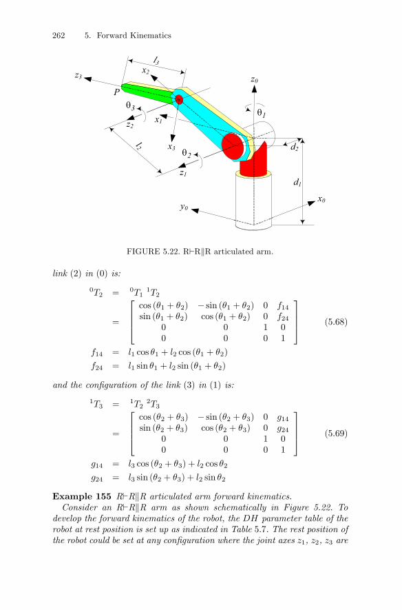
FIGURE 5.22. R`RkR articulated arm.
link (2) in (0) is:
0T2 = 0T11T2
=
⎡⎢⎢⎣cos (θ1 + θ2) − sin (θ1 + θ2) 0 f14sin (θ1 + θ2) cos (θ1 + θ2) 0 f24
0 0 1 00 0 0 1
⎤⎥⎥⎦ (5.68)
f14 = l1 cos θ1 + l2 cos (θ1 + θ2)
f24 = l1 sin θ1 + l2 sin (θ1 + θ2)
and the configuration of the link (3) in (1) is:
1T3 = 1T22T3
=
⎡⎢⎢⎣cos (θ2 + θ3) − sin (θ2 + θ3) 0 g14sin (θ2 + θ3) cos (θ2 + θ3) 0 g24
0 0 1 00 0 0 1
⎤⎥⎥⎦ (5.69)
g14 = l3 cos (θ2 + θ3) + l2 cos θ2
g24 = l3 sin (θ2 + θ3) + l2 sin θ2
Example 155 R`RkR articulated arm forward kinematics.Consider an R`RkR arm as shown schematically in Figure 5.22. To
develop the forward kinematics of the robot, the DH parameter table of therobot at rest position is set up as indicated in Table 5.7. The rest position ofthe robot could be set at any configuration where the joint axes z1, z2, z3 are
5. Forward Kinematics 263
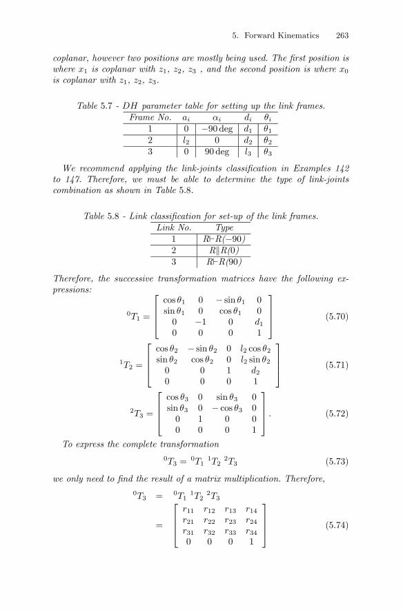
coplanar, however two positions are mostly being used. The first position iswhere x1 is coplanar with z1, z2, z3 , and the second position is where x0is coplanar with z1, z2, z3.
Table 5.7 - DH parameter table for setting up the link frames.Frame No. ai αi di θi
1 0 −90 deg d1 θ12 l2 0 d2 θ23 0 90 deg l3 θ3
We recommend applying the link-joints classification in Examples 142to 147. Therefore, we must be able to determine the type of link-jointscombination as shown in Table 5.8.
Table 5.8 - Link classification for set-up of the link frames.Link No. Type
1 R`R(−90)2 RkR(0)3 R`R(90)
Therefore, the successive transformation matrices have the following ex-pressions:
0T1 =
⎡⎢⎢⎣cos θ1 0 − sin θ1 0sin θ1 0 cos θ1 00 −1 0 d10 0 0 1
⎤⎥⎥⎦ (5.70)
1T2 =
⎡⎢⎢⎣cos θ2 − sin θ2 0 l2 cos θ2sin θ2 cos θ2 0 l2 sin θ20 0 1 d20 0 0 1
⎤⎥⎥⎦ (5.71)
2T3 =
⎡⎢⎢⎣cos θ3 0 sin θ3 0sin θ3 0 − cos θ3 00 1 0 00 0 0 1
⎤⎥⎥⎦ . (5.72)
To express the complete transformation
0T3 =0T1
1T22T3 (5.73)
we only need to find the result of a matrix multiplication. Therefore,
0T3 = 0T11T2
2T3
=
⎡⎢⎢⎣r11 r12 r13 r14r21 r22 r23 r24r31 r32 r33 r340 0 0 1
⎤⎥⎥⎦ (5.74)
264 5. Forward Kinematics
where
r11 = cos θ1 cos(θ2 + θ3) (5.75)
r21 = sin θ1 cos(θ2 + θ3) (5.76)
r31 = − sin(θ2 + θ3) (5.77)
r12 = − sin θ1 (5.78)
r22 = cos θ1 (5.79)
r32 = 0 (5.80)
r13 = cos θ1 sin(θ2 + θ3) (5.81)
r23 = sin θ1 sin(θ2 + θ3) (5.82)
r33 = cos(θ2 + θ3) (5.83)
r14 = l2 cos θ1 cos θ2 − d2 sin θ1 (5.84)
r24 = l2 cos θ2 sin θ1 + d2 cos θ1 (5.85)
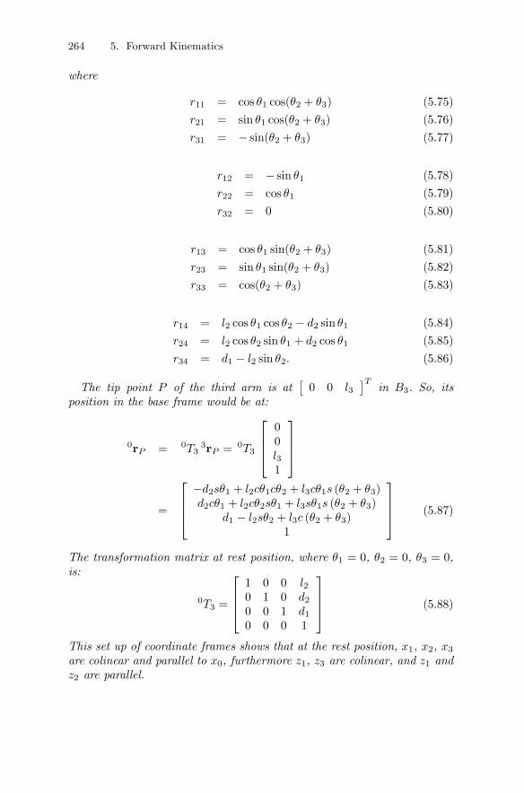
r34 = d1 − l2 sin θ2. (5.86)
The tip point P of the third arm is at£0 0 l3
¤Tin B3. So, its
position in the base frame would be at:
0rP = 0T33rP =
0T3
⎡⎢⎢⎣00l31
⎤⎥⎥⎦
=
⎡⎢⎢⎣−d2sθ1 + l2cθ1cθ2 + l3cθ1s (θ2 + θ3)d2cθ1 + l2cθ2sθ1 + l3sθ1s (θ2 + θ3)
d1 − l2sθ2 + l3c (θ2 + θ3)1
⎤⎥⎥⎦ (5.87)
The transformation matrix at rest position, where θ1 = 0, θ2 = 0, θ3 = 0,is:
0T3 =
⎡⎢⎢⎣1 0 0 l20 1 0 d20 0 1 d10 0 0 1
⎤⎥⎥⎦ (5.88)
This set up of coordinate frames shows that at the rest position, x1, x2, x3are colinear and parallel to x0, furthermore z1, z3 are colinear, and z1 andz2 are parallel.
5. Forward Kinematics 265
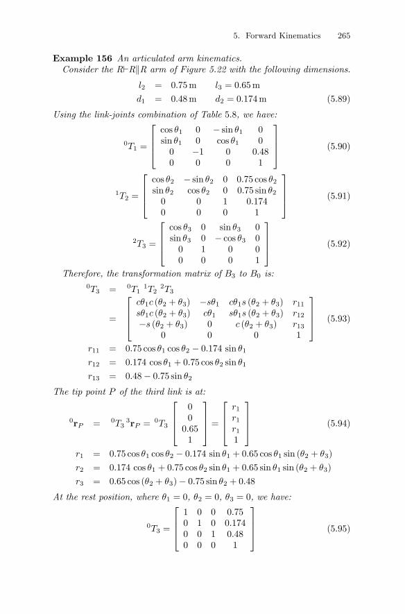
Example 156 An articulated arm kinematics.Consider the R`RkR arm of Figure 5.22 with the following dimensions.
l2 = 0.75m l3 = 0.65m
d1 = 0.48m d2 = 0.174m (5.89)
Using the link-joints combination of Table 5.8, we have:
0T1 =
⎡⎢⎢⎣cos θ1 0 − sin θ1 0sin θ1 0 cos θ1 00 −1 0 0.480 0 0 1
⎤⎥⎥⎦ (5.90)
1T2 =
⎡⎢⎢⎣cos θ2 − sin θ2 0 0.75 cos θ2sin θ2 cos θ2 0 0.75 sin θ20 0 1 0.1740 0 0 1
⎤⎥⎥⎦ (5.91)
2T3 =
⎡⎢⎢⎣cos θ3 0 sin θ3 0sin θ3 0 − cos θ3 00 1 0 00 0 0 1
⎤⎥⎥⎦ (5.92)
Therefore, the transformation matrix of B3 to B0 is:0T3 = 0T1
1T22T3
=
⎡⎢⎢⎣cθ1c (θ2 + θ3) −sθ1 cθ1s (θ2 + θ3) r11sθ1c (θ2 + θ3) cθ1 sθ1s (θ2 + θ3) r12−s (θ2 + θ3) 0 c (θ2 + θ3) r13
0 0 0 1
⎤⎥⎥⎦ (5.93)
r11 = 0.75 cos θ1 cos θ2 − 0.174 sin θ1r12 = 0.174 cos θ1 + 0.75 cos θ2 sin θ1
r13 = 0.48− 0.75 sin θ2The tip point P of the third link is at:
0rP = 0T33rP =
0T3
⎡⎢⎢⎣000.651
⎤⎥⎥⎦ =⎡⎢⎢⎣
r1r1r11
⎤⎥⎥⎦ (5.94)
r1 = 0.75 cos θ1 cos θ2 − 0.174 sin θ1 + 0.65 cos θ1 sin (θ2 + θ3)
r2 = 0.174 cos θ1 + 0.75 cos θ2 sin θ1 + 0.65 sin θ1 sin (θ2 + θ3)
r3 = 0.65 cos (θ2 + θ3)− 0.75 sin θ2 + 0.48At the rest position, where θ1 = 0, θ2 = 0, θ3 = 0, we have:
0T3 =
⎡⎢⎢⎣1 0 0 0.750 1 0 0.1740 0 1 0.480 0 0 1
⎤⎥⎥⎦ (5.95)
266 5. Forward Kinematics
that shows the tip point is at:
0rP =0T3
3rP =0T3
⎡⎢⎢⎣000.651
⎤⎥⎥⎦ =⎡⎢⎢⎣0.750.1741.131
⎤⎥⎥⎦ (5.96)
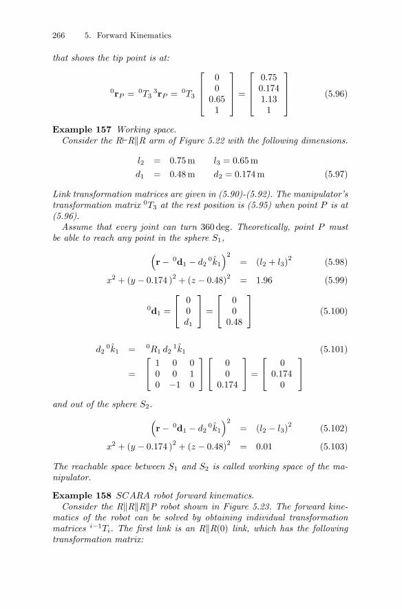
Example 157 Working space.Consider the R`RkR arm of Figure 5.22 with the following dimensions.
l2 = 0.75m l3 = 0.65m
d1 = 0.48m d2 = 0.174m (5.97)
Link transformation matrices are given in (5.90)-(5.92). The manipulator’stransformation matrix 0T3 at the rest position is (5.95) when point P is at(5.96).Assume that every joint can turn 360 deg. Theoretically, point P must
be able to reach any point in the sphere S1,³r− 0d1 − d2
0k1
´2= (l2 + l3)
2 (5.98)
x2 + (y − 0.174 )2 + (z − 0.48)2 = 1.96 (5.99)
0d1 =
⎡⎣ 00d1
⎤⎦ =⎡⎣ 0
00.48
⎤⎦ (5.100)
d20k1 = 0R1 d2
1k1 (5.101)
=
⎡⎣ 1 0 00 0 10 −1 0
⎤⎦⎡⎣ 00
0.174
⎤⎦ =⎡⎣ 00.1740
⎤⎦and out of the sphere S2.³
r− 0d1 − d20k1
´2= (l2 − l3)
2 (5.102)
x2 + (y − 0.174 )2 + (z − 0.48)2 = 0.01 (5.103)
The reachable space between S1 and S2 is called working space of the ma-nipulator.
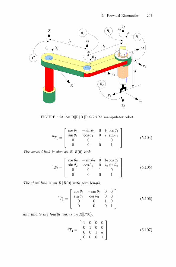
Example 158 SCARA robot forward kinematics.Consider the RkRkRkP robot shown in Figure 5.23. The forward kine-
matics of the robot can be solved by obtaining individual transformationmatrices i−1Ti. The first link is an RkR(0) link, which has the followingtransformation matrix:
5. Forward Kinematics 267
G
Z
l1
B2B1
x2
d
X
l2
z1
x1
x4
x3
z3z2
z4
y4
B3
B4
3θ
2θ
1θ
FIGURE 5.23. An RkRkRkP SCARA manipulator robot.
0T1 =
⎡⎢⎢⎣cos θ1 − sin θ1 0 l1 cos θ1sin θ1 cos θ1 0 l1 sin θ10 0 1 00 0 0 1
⎤⎥⎥⎦ (5.104)
The second link is also an RkR(0) link.
1T2 =
⎡⎢⎢⎣cos θ2 − sin θ2 0 l2 cos θ2sin θ2 cos θ2 0 l2 sin θ20 0 1 00 0 0 1
⎤⎥⎥⎦ (5.105)
The third link is an RkR(0) with zero length
2T3 =
⎡⎢⎢⎣cos θ3 − sin θ3 0 0sin θ3 cos θ3 0 00 0 1 00 0 0 1
⎤⎥⎥⎦ (5.106)
and finally the fourth link is an RkP(0).
3T4 =
⎡⎢⎢⎣1 0 0 00 1 0 00 0 1 d0 0 0 1
⎤⎥⎥⎦ (5.107)
268 5. Forward Kinematics
Therefore, the configuration of the end-effector in the base coordinate frameis
0T4 = 0T11T2
2T33T4 (5.108)
=
⎡⎢⎢⎣c(θ1 + θ2 + θ3) −s(θ1 + θ2 + θ3) 0 l1cθ1 + l2c(θ1 + θ2)s(θ1 + θ2 + θ3) c(θ1 + θ2 + θ3) 0 l1sθ1 + l2s(θ1 + θ2)
0 0 1 d0 0 0 1
⎤⎥⎥⎦that shows the rest position of the robot θ1 = θ2 = θ3 = d = 0 is at:
0T4 =
⎡⎢⎢⎣1 0 0 l1 + l20 1 0 00 0 1 00 0 0 1
⎤⎥⎥⎦ (5.109)
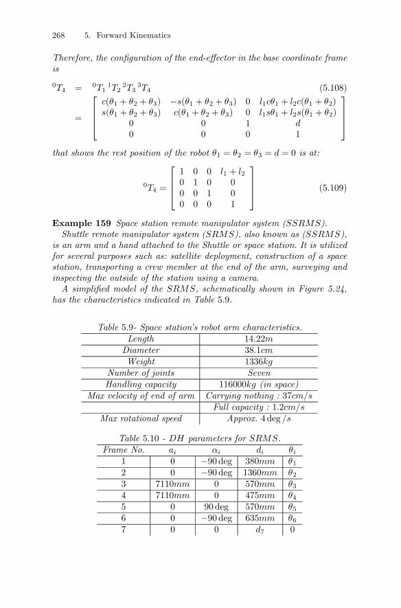
Example 159 Space station remote manipulator system (SSRMS).Shuttle remote manipulator system (SRMS), also known as (SSRMS),
is an arm and a hand attached to the Shuttle or space station. It is utilizedfor several purposes such as: satellite deployment, construction of a spacestation, transporting a crew member at the end of the arm, surveying andinspecting the outside of the station using a camera.A simplified model of the SRMS, schematically shown in Figure 5.24,
has the characteristics indicated in Table 5.9.
Table 5.9- Space station’s robot arm characteristics.Length 14.22mDiameter 38.1cmWeight 1336kg
Number of joints SevenHandling capacity 116000kg (in space)
Max velocity of end of arm Carrying nothing : 37cm/sFull capacity : 1.2cm/s
Max rotational speed Approx. 4 deg /s
Table 5.10 - DH parameters for SRMS.Frame No. ai αi di θi
1 0 −90 deg 380mm θ12 0 −90 deg 1360mm θ23 7110mm 0 570mm θ34 7110mm 0 475mm θ45 0 90 deg 570mm θ56 0 −90 deg 635mm θ67 0 0 d7 0
5. Forward Kinematics 269
z0
x5
Shoulder joints
Elbow joint
Wrist jointsz1
z2
z3
z4
z5
z6
z7
x0 y0
x1
x3
x4
x6
y7
x2
x7
3θ1θ
2θ
4θ
5θ
6θ 7θ
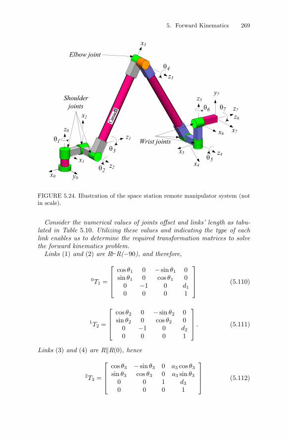
FIGURE 5.24. Illustration of the space station remote manipulator system (notin scale).
Consider the numerical values of joints offset and links’ length as tabu-lated in Table 5.10. Utilizing these values and indicating the type of eachlink enables us to determine the required transformation matrices to solvethe forward kinematics problem.Links (1) and (2) are R`R(−90), and therefore,
0T1 =
⎡⎢⎢⎣cos θ1 0 − sin θ1 0sin θ1 0 cos θ1 00 −1 0 d10 0 0 1
⎤⎥⎥⎦ (5.110)
1T2 =
⎡⎢⎢⎣cos θ2 0 − sin θ2 0sin θ2 0 cos θ2 00 −1 0 d20 0 0 1
⎤⎥⎥⎦ . (5.111)
Links (3) and (4) are RkR(0), hence
2T3 =
⎡⎢⎢⎣cos θ3 − sin θ3 0 a3 cos θ3sin θ3 cos θ3 0 a3 sin θ30 0 1 d30 0 0 1
⎤⎥⎥⎦ (5.112)
270 5. Forward Kinematics
3T4 =
⎡⎢⎢⎣cos θ4 − sin θ4 0 a4 cos θ4sin θ4 cos θ4 0 a4 sin θ40 0 1 d40 0 0 1
⎤⎥⎥⎦ . (5.113)
Link (5) is R`R(90), and link (6) is R`R(−90), therefore
4T5 =
⎡⎢⎢⎣cos θ5 0 sin θ5 0sin θ5 0 − cos θ5 00 1 0 d50 0 0 1
⎤⎥⎥⎦ (5.114)
5T6 =
⎡⎢⎢⎣cos θ6 0 − sin θ6 0sin θ6 0 cos θ6 00 −1 0 d60 0 0 1
⎤⎥⎥⎦ . (5.115)
Finally link (7) is R`R(0) and the coordinate frame attached to the end-effector has a translation d7 with respect to the coordinate frame B6.
6T7 =
⎡⎢⎢⎣cos θ7 − sin θ7 0 0sin θ7 cos θ7 0 00 0 1 d70 0 0 1
⎤⎥⎥⎦ (5.116)
The forward kinematics of SSRMS can be found by direct multiplicationof i−1Ti, (i = 1, 2, · · · , 7).
0T7 =0T1
1T22T3
3T44T5
5T66T7 (5.117)
5.4 Spherical Wrist
Figure 5.25 illustrates a spherical joint . The spherical joint connects twolinks: the forearm and hand. The axis of the forearm and hand are assumedto be colinear at the rest position. The axis of the hand is called the gripperaxis. A spherical wrist is a combination of links and joints to simulate aspherical joint and provide three rotational DOF for the gripper link. Itis made by three R`R links with zero lengths and zero offset where theirjoint axes are mutually orthogonal and intersecting at a point called thewrist point . The wrist point is invariant in a robot structure and will notmove by wrist angular coordinates.At the wrist point, we define two coordinate frames. The first is the wrist
dead frame, attached to the forearm link, and the second frame is the wristliving frame, attached to the hand link. We also introduce a tool or gripperframe. The tool frame of the wrist is denoted by three vectors, a ≡ k, s ≡ ı,
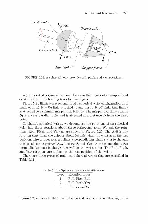
5. Forward Kinematics 271
Yaw
Pitch
Roll a
n
s
Gripper axis
Gripper frame
Forearm link
Hand link
Wrist point
FIGURE 5.25. A spherical joint provides roll, pitch, and yaw rotations.
n ≡ j. It is set at a symmetric point between the fingers of an empty handor at the tip of the holding tools by the fingers.Figure 5.26 illustrates a schematic of a spherical wrist configuration. It is
made of an R`R(−90) link, attached to another R`R(90) link, that finallyis attached to a spinning gripper link RkR(0). The gripper coordinate frameB7 is always parallel to B6 and is attached at a distance d7 from the wristpoint.To classify spherical wrists, we decompose the rotations of an spherical
wrist into three rotations about three orthogonal axes. We call the rota-tions, Roll, Pitch, and Yaw as are shown in Figure 5.25. The Roll is anyrotation that turns the gripper about its axis when the wrist is at the restposition. The gripper axis a defines a perpendicular plane s× n to the axisthat is called the gripper wall. The Pitch and Yaw are rotations about twoperpendicular axes in the gripper wall at the wrist point. The Roll, Pitch,and Yaw rotations are defined at the rest position of the wrist.There are three types of practical spherical wrists that are classified in
Table 5.11.
Table 5.11 - Spherical wrists classification.Type Rotation order1 Roll-Pitch-Roll2 Roll-Pitch-Yaw3 Pitch-Yaw-Roll
Figure 5.26 shows a Roll-Pitch-Roll spherical wrist with the following trans-
272 5. Forward Kinematics
B3
z3
z5
z4
Attached to forearm
x5
z7
x7
y7
d7
x3 z6
x6
Gripper
x4
4θ5θ
6θ
B4
B5
Wrist point
B6
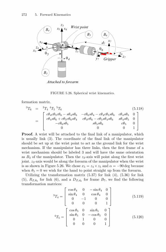
FIGURE 5.26. Spherical wrist kinematics.
formation matrix.3T6 = 3T4
4T55T6 (5.118)
=
⎡⎢⎢⎣cθ4cθ5cθ6 − sθ4sθ6 −cθ6sθ4 − cθ4cθ5sθ6 cθ4sθ5 0cθ4sθ6 + cθ5cθ6sθ4 cθ4cθ6 − cθ5sθ4sθ6 sθ4sθ5 0
−cθ6sθ5 sθ5sθ6 cθ5 00 0 0 1
⎤⎥⎥⎦Proof. A wrist will be attached to the final link of a manipulator, whichis usually link (3). The coordinate of the final link of the manipulatorshould be set up at the wrist point to act as the ground link for the wristmechanism. If the manipulator has three links, then the first frame of awrist mechanism should be labeled 3 and will have the same orientationas B3 of the manipulator. Then the z3-axis will point along the first wristjoint. z3-axis would be along the forearm of the manipulator when the wristis as shown in Figure 5.26. We chose x5 = z4×z5 and α = −90 deg becausewhen θ5 = 0 we wish for the hand to point straight up from the forearm.Utilizing the transformation matrix (5.37) for link (4), (5.36) for link
(5), RZ,θ6 for link (6), and a DZ,d6 for frame B7, we find the followingtransformation matrices:
3T4 =
⎡⎢⎢⎣cos θ4 0 − sin θ4 0sin θ4 0 cos θ4 00 −1 0 00 0 0 1
⎤⎥⎥⎦ (5.119)
4T5 =
⎡⎢⎢⎣cos θ5 0 sin θ5 0sin θ5 0 − cos θ5 00 1 0 00 0 0 1
⎤⎥⎥⎦ (5.120)
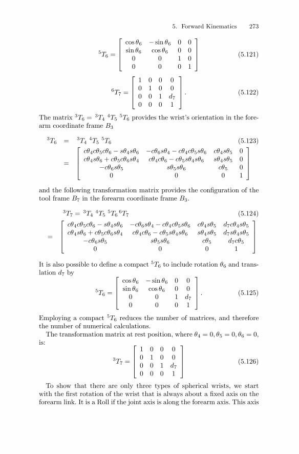
5. Forward Kinematics 273
5T6 =
⎡⎢⎢⎣cos θ6 − sin θ6 0 0sin θ6 cos θ6 0 00 0 1 00 0 0 1
⎤⎥⎥⎦ (5.121)
6T7 =
⎡⎢⎢⎣1 0 0 00 1 0 00 0 1 d70 0 0 1
⎤⎥⎥⎦ . (5.122)
The matrix 3T6 =3T4
4T55T6 provides the wrist’s orientation in the fore-
arm coordinate frame B3
3T6 = 3T44T5
5T6 (5.123)
=
⎡⎢⎢⎣cθ4cθ5cθ6 − sθ4sθ6 −cθ6sθ4 − cθ4cθ5sθ6 cθ4sθ5 0cθ4sθ6 + cθ5cθ6sθ4 cθ4cθ6 − cθ5sθ4sθ6 sθ4sθ5 0
−cθ6sθ5 sθ5sθ6 cθ5 00 0 0 1
⎤⎥⎥⎦and the following transformation matrix provides the configuration of thetool frame B7 in the forearm coordinate frame B3.
3T7 =3T4
4T55T6
6T7 (5.124)
=
⎡⎢⎢⎣cθ4cθ5cθ6 − sθ4sθ6 −cθ6sθ4 − cθ4cθ5sθ6 cθ4sθ5 d7cθ4sθ5cθ4sθ6 + cθ5cθ6sθ4 cθ4cθ6 − cθ5sθ4sθ6 sθ4sθ5 d7sθ4sθ5
−cθ6sθ5 sθ5sθ6 cθ5 d7cθ50 0 0 1
⎤⎥⎥⎦It is also possible to define a compact 5T6 to include rotation θ6 and trans-lation d7 by
5T6 =
⎡⎢⎢⎣cos θ6 − sin θ6 0 0sin θ6 cos θ6 0 00 0 1 d70 0 0 1
⎤⎥⎥⎦ . (5.125)
Employing a compact 5T6 reduces the number of matrices, and thereforethe number of numerical calculations.The transformation matrix at rest position, where θ4 = 0, θ5 = 0, θ6 = 0,
is:
3T7 =
⎡⎢⎢⎣1 0 0 00 1 0 00 0 1 d70 0 0 1
⎤⎥⎥⎦ (5.126)
To show that there are only three types of spherical wrists, we startwith the first rotation of the wrist that is always about a fixed axis on theforearm link. It is a Roll if the joint axis is along the forearm axis. This axis
274 5. Forward Kinematics
z7
z3
d7
z4 a
s
n
z5
x3
x7
y7
x5 x6
z6
x4
4θ
5θ
6θ
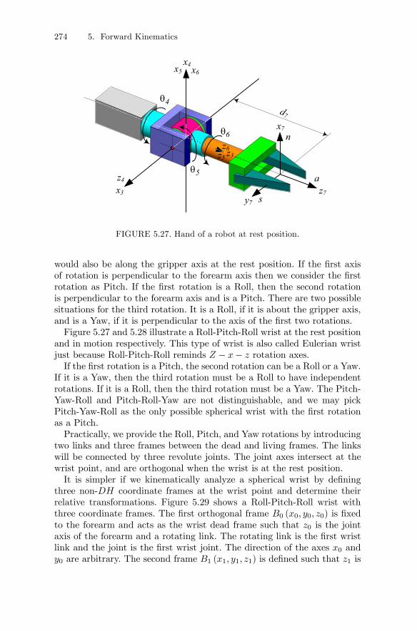
FIGURE 5.27. Hand of a robot at rest position.
would also be along the gripper axis at the rest position. If the first axisof rotation is perpendicular to the forearm axis then we consider the firstrotation as Pitch. If the first rotation is a Roll, then the second rotationis perpendicular to the forearm axis and is a Pitch. There are two possiblesituations for the third rotation. It is a Roll, if it is about the gripper axis,and is a Yaw, if it is perpendicular to the axis of the first two rotations.Figure 5.27 and 5.28 illustrate a Roll-Pitch-Roll wrist at the rest position
and in motion respectively. This type of wrist is also called Eulerian wristjust because Roll-Pitch-Roll reminds Z − x− z rotation axes.If the first rotation is a Pitch, the second rotation can be a Roll or a Yaw.
If it is a Yaw, then the third rotation must be a Roll to have independentrotations. If it is a Roll, then the third rotation must be a Yaw. The Pitch-Yaw-Roll and Pitch-Roll-Yaw are not distinguishable, and we may pickPitch-Yaw-Roll as the only possible spherical wrist with the first rotationas a Pitch.Practically, we provide the Roll, Pitch, and Yaw rotations by introducing
two links and three frames between the dead and living frames. The linkswill be connected by three revolute joints. The joint axes intersect at thewrist point, and are orthogonal when the wrist is at the rest position.It is simpler if we kinematically analyze a spherical wrist by defining
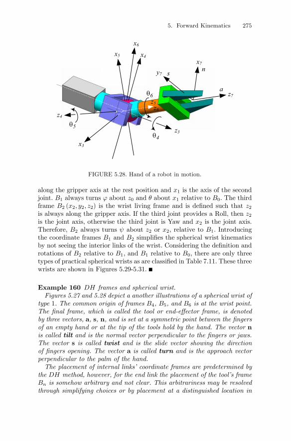
three non-DH coordinate frames at the wrist point and determine theirrelative transformations. Figure 5.29 shows a Roll-Pitch-Roll wrist withthree coordinate frames. The first orthogonal frame B0 (x0, y0, z0) is fixedto the forearm and acts as the wrist dead frame such that z0 is the jointaxis of the forearm and a rotating link. The rotating link is the first wristlink and the joint is the first wrist joint. The direction of the axes x0 andy0 are arbitrary. The second frame B1 (x1, y1, z1) is defined such that z1 is
5. Forward Kinematics 275
z7
z3
z4
a
s n
z5
x3
x7
y7
x5 x4
z6
x6
4θ5θ
6θ
FIGURE 5.28. Hand of a robot in motion.
along the gripper axis at the rest position and x1 is the axis of the secondjoint. B1 always turns ϕ about z0 and θ about x1 relative to B0. The thirdframe B2 (x2, y2, z2) is the wrist living frame and is defined such that z2is always along the gripper axis. If the third joint provides a Roll, then z2is the joint axis, otherwise the third joint is Yaw and x2 is the joint axis.Therefore, B2 always turns ψ about z2 or x2, relative to B1. Introducingthe coordinate frames B1 and B2 simplifies the spherical wrist kinematicsby not seeing the interior links of the wrist. Considering the definition androtations of B2 relative to B1, and B1 relative to B0, there are only threetypes of practical spherical wrists as are classified in Table 7.11. These threewrists are shown in Figures 5.29-5.31.
Example 160 DH frames and spherical wrist.Figures 5.27 and 5.28 depict a another illustrations of a spherical wrist of
type 1. The common origin of frames B4, B5, and B6 is at the wrist point.The final frame, which is called the tool or end-effector frame, is denotedby three vectors, a, s, n, and is set at a symmetric point between the fingersof an empty hand or at the tip of the tools hold by the hand. The vector nis called tilt and is the normal vector perpendicular to the fingers or jaws.The vector s is called twist and is the slide vector showing the directionof fingers opening. The vector a is called turn and is the approach vectorperpendicular to the palm of the hand.The placement of internal links’ coordinate frames are predetermined by
the DH method, however, for the end link the placement of the tool’s frameBn is somehow arbitrary and not clear. This arbitrariness may be resolvedthrough simplifying choices or by placement at a distinguished location in
276 5. Forward Kinematics
x1
z2
x0
z0
B0 B1
ϕ
θ
ψ
B2
z1
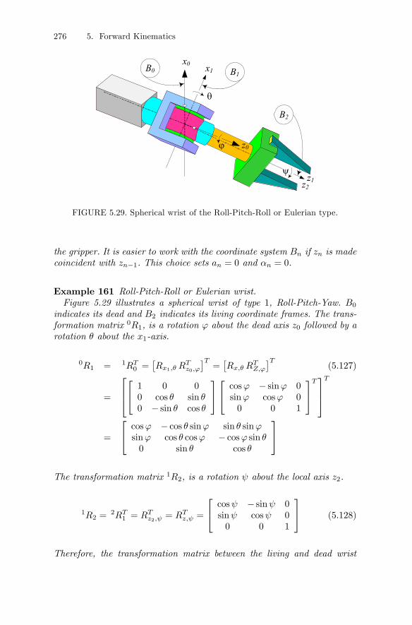
FIGURE 5.29. Spherical wrist of the Roll-Pitch-Roll or Eulerian type.
the gripper. It is easier to work with the coordinate system Bn if zn is madecoincident with zn−1. This choice sets an = 0 and αn = 0.
Example 161 Roll-Pitch-Roll or Eulerian wrist.Figure 5.29 illustrates a spherical wrist of type 1, Roll-Pitch-Yaw. B0
indicates its dead and B2 indicates its living coordinate frames. The trans-formation matrix 0R1, is a rotation ϕ about the dead axis z0 followed by arotation θ about the x1-axis.
0R1 = 1RT0 =
£Rx1,θ R
Tz0,ϕ
¤T=£Rx,θ R
TZ,ϕ
¤T(5.127)
=
⎡⎢⎣⎡⎣ 1 0 00 cos θ sin θ0 − sin θ cos θ
⎤⎦⎡⎣ cosϕ − sinϕ 0sinϕ cosϕ 00 0 1
⎤⎦T⎤⎥⎦T
=
⎡⎣ cosϕ − cos θ sinϕ sin θ sinϕsinϕ cos θ cosϕ − cosϕ sin θ0 sin θ cos θ
⎤⎦The transformation matrix 1R2, is a rotation ψ about the local axis z2.
1R2 =2RT
1 = RTz2,ψ = RT
z,ψ =
⎡⎣ cosψ − sinψ 0sinψ cosψ 00 0 1
⎤⎦ (5.128)
Therefore, the transformation matrix between the living and dead wrist
5. Forward Kinematics 277
x0
x2 x1
B0
B1
ϕ
θ
ψ
z0 z1
B2
z2
FIGURE 5.30. Spherical wrist of the Roll-Pitch-Yaw type.
frames is:
0R2 = 0R11R2 =
£Rx1,θ R
Tz0,ϕ
¤TRTz2,ψ = Rz0,ϕR
Tx1,θ R
Tz2,ψ
= RZ,ϕRTx,θ R
Tz,ψ (5.129)
=
⎡⎣ cψcϕ− cθsψsϕ −cϕsψ − cθcψsϕ sθsϕcψsϕ+ cθcϕsψ cθcψcϕ− sψsϕ −cϕsθ
sθsψ cψsθ cθ
⎤⎦
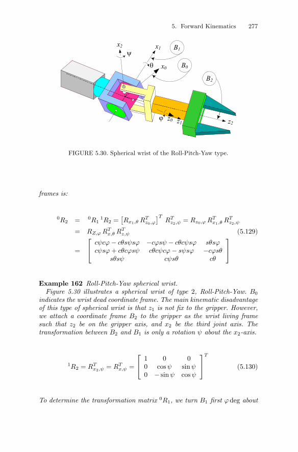
Example 162 Roll-Pitch-Yaw spherical wrist.Figure 5.30 illustrates a spherical wrist of type 2, Roll-Pitch-Yaw. B0
indicates the wrist dead coordinate frame. The main kinematic disadvantageof this type of spherical wrist is that z1 is not fix to the gripper. However,we attach a coordinate frame B2 to the gripper as the wrist living framesuch that z2 be on the gripper axis, and x2 be the third joint axis. Thetransformation between B2 and B1 is only a rotation ψ about the x2-axis.
1R2 = RTx2,ψ = RT
x,ψ =
⎡⎣ 1 0 00 cosψ sinψ0 − sinψ cosψ
⎤⎦T (5.130)
To determine the transformation matrix 0R1, we turn B1 first ϕdeg about
278 5. Forward Kinematics
-z0
x0x1
B0
θ
ϕ
z2
ψ
B1
B2
FIGURE 5.31. Spherical wrist of the Pitch-Yaw-Roll type.
the z0-axis, then θ deg about the x1-axis.
0R1 = 1RT0 =
£Rx1,θ R
Tz0,ϕ
¤T=£Rx,θ R
TZ,ϕ
¤T(5.131)
=
⎡⎢⎣⎡⎣ 1 0 00 cθ sθ0 −sθ cθ
⎤⎦⎡⎣ cϕ −sϕ 0sϕ cϕ 00 0 1
⎤⎦T⎤⎥⎦T
=
⎡⎣ cosϕ − cos θ sinϕ sin θ sinϕsinϕ cos θ cosϕ − cosϕ sin θ0 sin θ cos θ
⎤⎦Therefore, the transformation matrix between the living and dead wristframes is:
0R2 = 0R11R2 =
£Rx1,θ R
Tz0,ϕ
¤TRTx2,ψ = Rz0,ϕR
Tx1,θ R
Tx2,ψ
= RZ,ϕRTx,θ R
Tx,ψ (5.132)
=
⎡⎣ cϕ sθsψsϕ− cθcψsϕ cθsψsϕ+ cψsθsϕsϕ cθcψcϕ− cϕsθsψ −cθcϕsψ − cψcϕsθ0 cθsψ + cψsθ cθcψ − sθsψ
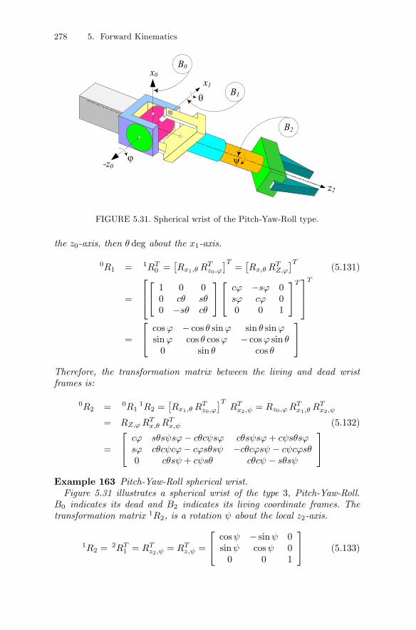
⎤⎦Example 163 Pitch-Yaw-Roll spherical wrist.Figure 5.31 illustrates a spherical wrist of the type 3, Pitch-Yaw-Roll.
B0 indicates its dead and B2 indicates its living coordinate frames. Thetransformation matrix 1R2, is a rotation ψ about the local z2-axis.
1R2 =2RT
1 = RTz2,ψ = RT
z,ψ =
⎡⎣ cosψ − sinψ 0sinψ cosψ 00 0 1
⎤⎦ (5.133)
5. Forward Kinematics 279
B6
B4
B5
z4
z6
z5
FIGURE 5.32. A practical spherical wrist.
To determine the transformation matrix 0R1, we turn B1 first ϕdeg aboutthe z0-axis, and then θ deg about the x1-axis.
0R1 = 1RT0 =
£Rx1,θ R
Tz0,ϕ
¤T=£Rx,θ R
TZ,ϕ
¤T(5.134)
=
⎡⎢⎣⎡⎣ 1 0 00 cθ sθ0 −sθ cθ
⎤⎦⎡⎣ cϕ −sϕ 0sϕ cϕ 00 0 1
⎤⎦T⎤⎥⎦T
=
⎡⎣ cosϕ − cos θ sinϕ sin θ sinϕsinϕ cos θ cosϕ − cosϕ sin θ0 sin θ cos θ
⎤⎦Therefore, the transformation matrix between the living and dead wristframes is:
0R2 = 0R11R2 =
£Rx1,θ R
Tz0,ϕ
¤TRTz2,ψ = Rz0,ϕR
Tx1,θ R
Tz2,ψ
= RZ,ϕRTx,θ R
Tz,ψ (5.135)
=
⎡⎣ cψcϕ− cθsψsϕ −cϕsψ − cθcψsϕ sθsϕcψsϕ+ cθcϕsψ cθcψcϕ− sψsϕ −cϕsθ
sθsψ cψsθ cθ
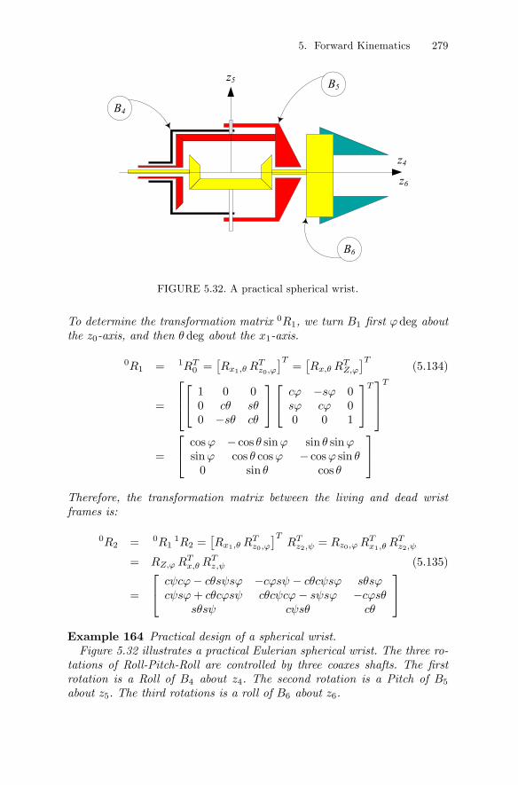
⎤⎦Example 164 Practical design of a spherical wrist.Figure 5.32 illustrates a practical Eulerian spherical wrist. The three ro-
tations of Roll-Pitch-Roll are controlled by three coaxes shafts. The firstrotation is a Roll of B4 about z4. The second rotation is a Pitch of B5about z5. The third rotations is a roll of B6 about z6.
280 5. Forward Kinematics
z0
Base
Shoulder
Elbow
Forearm
z1
z3
x3
l2
x0z2
d2
l8
y1
1θ
2θ
3θ
B0
B1
B2
B3
M1
M2 M3
x8
z8
B8
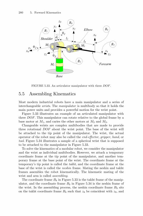
FIGURE 5.33. An articulator manipulator with three DOF .
5.5 Assembling Kinematics
Most modern industrial robots have a main manipulator and a series ofinterchangeable wrists. The manipulator is multibody so that it holds themain power units and provides a powerful motion for the wrist point.Figure 5.33 illustrates an example of an articulated manipulator with
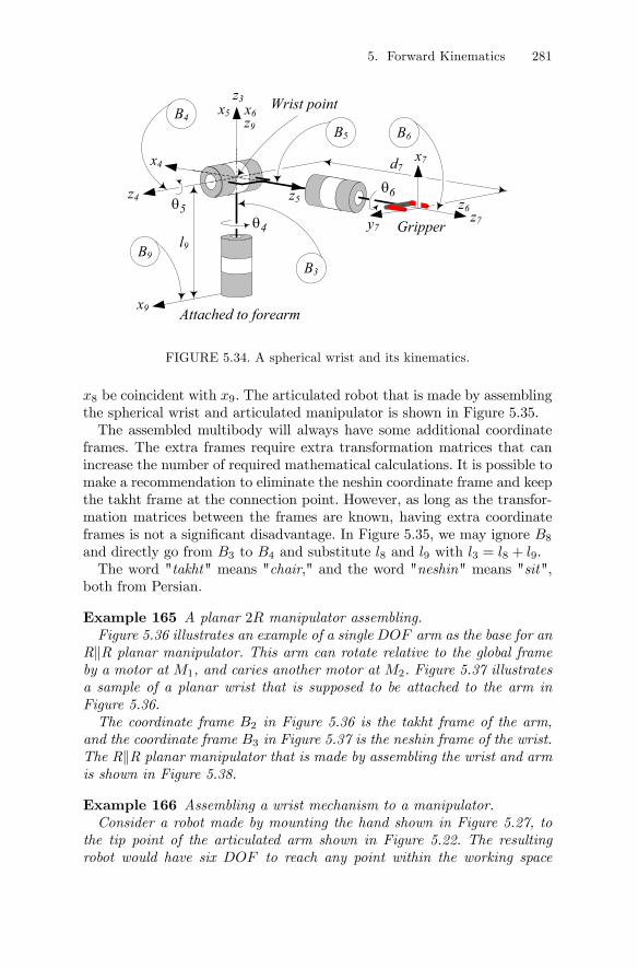
three DOF . This manipulator can rotate relative to the global frame by abase motor at M1, and caries the other motors at M2 and M3.Changeable wrists are complex multibodies that are made to provide
three rotational DOF about the wrist point. The base of the wrist willbe attached to the tip point of the manipulator. The wrist, the actualoperator of the robot may also be called the end-effector, gripper, hand, ortool. Figure 5.34 illustrates a sample of a spherical wrist that is supposedto be attached to the manipulator in Figure 5.33.To solve the kinematics of a modular robot, we consider the manipulator
and the wrist as individual multibodies. However, we attach a temporarycoordinate frame at the tip point of the manipulator, and another tem-porary frame at the base point of the wrist. The coordinate frame at thetemporary’s tip point is called the takht, and the coordinate frame at thebase of the wrist is called the neshin frame. Mating the neshin and takhtframes assembles the robot kinematically. The kinematic mating of thewrist and arm is called assembling.The coordinate frame B8 in Figure 5.33 is the takht frame of the manip-
ulator, and the coordinate frame B9 in Figure 5.34 is the neshin frame ofthe wrist. In the assembling process, the neshin coordinate frame B9 sitson the takht coordinate frame B8 such that z8 be coincident with z9, and
5. Forward Kinematics 281
B9
z3
z5z4
Attached to forearm
x5
z7
x7
y7
d7
z6
x6
Gripper
x4
4θ5θ
6θ
B4
B5
Wrist point
B6
x9
z9
B3
l9
FIGURE 5.34. A spherical wrist and its kinematics.
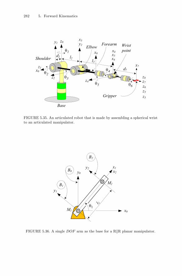
x8 be coincident with x9. The articulated robot that is made by assemblingthe spherical wrist and articulated manipulator is shown in Figure 5.35.The assembled multibody will always have some additional coordinate
frames. The extra frames require extra transformation matrices that canincrease the number of required mathematical calculations. It is possible tomake a recommendation to eliminate the neshin coordinate frame and keepthe takht frame at the connection point. However, as long as the transfor-mation matrices between the frames are known, having extra coordinateframes is not a significant disadvantage. In Figure 5.35, we may ignore B8and directly go from B3 to B4 and substitute l8 and l9 with l3 = l8 + l9.The word "takht" means "chair," and the word "neshin" means "sit",
both from Persian.
Example 165 A planar 2R manipulator assembling.Figure 5.36 illustrates an example of a single DOF arm as the base for an
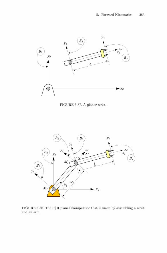
RkR planar manipulator. This arm can rotate relative to the global frameby a motor at M1, and caries another motor at M2. Figure 5.37 illustratesa sample of a planar wrist that is supposed to be attached to the arm inFigure 5.36.The coordinate frame B2 in Figure 5.36 is the takht frame of the arm,
and the coordinate frame B3 in Figure 5.37 is the neshin frame of the wrist.The RkR planar manipulator that is made by assembling the wrist and armis shown in Figure 5.38.
Example 166 Assembling a wrist mechanism to a manipulator.Consider a robot made by mounting the hand shown in Figure 5.27, to
the tip point of the articulated arm shown in Figure 5.22. The resultingrobot would have six DOF to reach any point within the working space
282 5. Forward Kinematics
z0
Base
Shoulder
ElbowForearm
z1
z5
z4
z6
x3
z3
x5x6
x4
z7
x7d7
Gripper
l2
Wrist point
y2
x0
z2
d2
l3
y1
1θ
2θ3θ
4θ
5θ 6θ
x8
z8
FIGURE 5.35. An articulated robot that is made by assembling a spherical wristto an articulated manipulator.
y0
y2x2
x01θ
B0
B1
M1
M2
y1
x1
B2
l 1
FIGURE 5.36. A single DOF arm as the base for a RkR planar manipulator.
5. Forward Kinematics 283
x4
y4
y0
y3
x3
x0
B0
B3
B4
l2
FIGURE 5.37. A planar wrist.
y0
y2x2
x01θ
B0
B1
M1
M2
y1
x1
B2
l 1
x4
y4
y3
x3
B3
B4
l2
FIGURE 5.38. The RkR planar manipulator that is made by assembling a wristand an arm.
284 5. Forward Kinematics
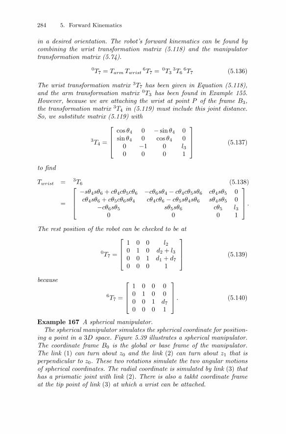
in a desired orientation. The robot’s forward kinematics can be found bycombining the wrist transformation matrix (5.118) and the manipulatortransformation matrix (5.74).
0T7 = Tarm Twrist6T7 =
0T33T6
6T7 (5.136)
The wrist transformation matrix 3T7 has been given in Equation (5.118),and the arm transformation matrix 0T3 has been found in Example 155.However, because we are attaching the wrist at point P of the frame B3,the transformation matrix 3T4 in (5.119) must include this joint distance.So, we substitute matrix (5.119) with
3T4 =
⎡⎢⎢⎣cos θ4 0 − sin θ4 0sin θ4 0 cos θ4 00 −1 0 l30 0 0 1
⎤⎥⎥⎦ (5.137)
to find
Twrist = 3T6 (5.138)
=
⎡⎢⎢⎣−sθ4sθ6 + cθ4cθ5cθ6 −cθ6sθ4 − cθ4cθ5sθ6 cθ4sθ5 0cθ4sθ6 + cθ5cθ6sθ4 cθ4cθ6 − cθ5sθ4sθ6 sθ4sθ5 0
−cθ6sθ5 sθ5sθ6 cθ5 l30 0 0 1
⎤⎥⎥⎦ .The rest position of the robot can be checked to be at
0T7 =
⎡⎢⎢⎣1 0 0 l20 1 0 d2 + l30 0 1 d1 + d70 0 0 1
⎤⎥⎥⎦ (5.139)
because
6T7 =
⎡⎢⎢⎣1 0 0 00 1 0 00 0 1 d70 0 0 1
⎤⎥⎥⎦ . (5.140)
Example 167 A spherical manipulator.The spherical manipulator simulates the spherical coordinate for position-
ing a point in a 3D space. Figure 5.39 illustrates a spherical manipulator.The coordinate frame B0 is the global or base frame of the manipulator.The link (1) can turn about z0 and the link (2) can turn about z1 that isperpendicular to z0. These two rotations simulate the two angular motionsof spherical coordinates. The radial coordinate is simulated by link (3) thathas a prismatic joint with link (2). There is also a takht coordinate frameat the tip point of link (3) at which a wrist can be attached.
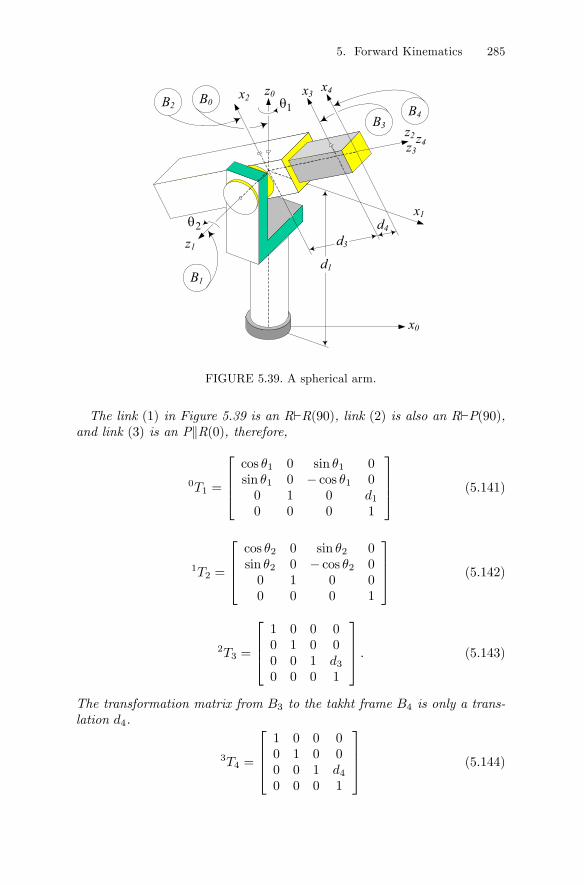
5. Forward Kinematics 285
x0
z0
z1
2θx1
1θ
z2
x2 x3
z3
x4
d4
B0
B1
z4
B2
B3B4
d1
d3
FIGURE 5.39. A spherical arm.
The link (1) in Figure 5.39 is an R`R(90), link (2) is also an R`P(90),and link (3) is an PkR(0), therefore,
0T1 =
⎡⎢⎢⎣cos θ1 0 sin θ1 0sin θ1 0 − cos θ1 00 1 0 d10 0 0 1
⎤⎥⎥⎦ (5.141)
1T2 =
⎡⎢⎢⎣cos θ2 0 sin θ2 0sin θ2 0 − cos θ2 00 1 0 00 0 0 1
⎤⎥⎥⎦ (5.142)
2T3 =
⎡⎢⎢⎣1 0 0 00 1 0 00 0 1 d30 0 0 1
⎤⎥⎥⎦ . (5.143)
The transformation matrix from B3 to the takht frame B4 is only a trans-lation d4.
3T4 =
⎡⎢⎢⎣1 0 0 00 1 0 00 0 1 d40 0 0 1
⎤⎥⎥⎦ (5.144)
286 5. Forward Kinematics
x0
z0
z1
2θ
x1
1θ
z2
x2 x3
z3
x4
d4
B0
B1
z4
B2
B3B4
d1
d3
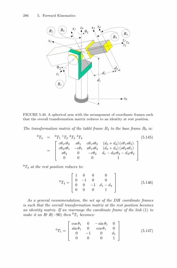
FIGURE 5.40. A spherical arm with the arrangement of coordinate frames suchthat the overall transformation matrix reduces to an identity at rest position.
The transformation matrix of the takht frame B4 to the base frame B0 is:
0T4 = 0T11T2
2T33T4 (5.145)
=
⎡⎢⎢⎣cθ1cθ2 sθ1 cθ1sθ2 (d3 + d4) (cθ1sθ2)cθ2sθ1 −cθ1 sθ1sθ2 (d3 + d4) (sθ2sθ1)sθ2 0 −cθ2 d1 − d3cθ2 − d4cθ20 0 0 1
⎤⎥⎥⎦0T4 at the rest position reduces to:
0T4 =
⎡⎢⎢⎣1 0 0 00 −1 0 00 0 −1 d1 − d40 0 0 1
⎤⎥⎥⎦ (5.146)
As a general recommendation, the set up of the DH coordinate framesis such that the overall transformation matrix at the rest position becomesan identity matrix. If we rearrange the coordinate frame of the link (1) tomake it an R`R(−90) then 0T1 becomes:
0T1 =
⎡⎢⎢⎣cos θ1 0 − sin θ1 0sin θ1 0 cos θ1 00 −1 0 d10 0 0 1
⎤⎥⎥⎦ (5.147)
5. Forward Kinematics 287
z6
7θ
z5
x6
z9
x9
6θ
x7
z8
B5
B6
B8
8θ
x8 x5
z7
d5
B7B9
x0
z0
z1
2θ
x1
1θ
z2x2
x3 z3x4
d4
B0B1
z4B2
B3B4
d1
d3
d9
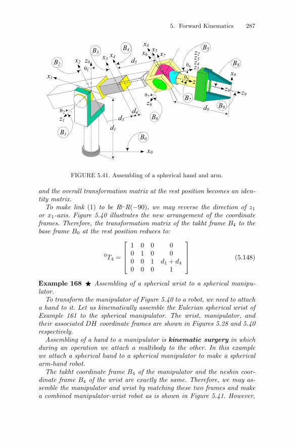
FIGURE 5.41. Assembling of a spherical hand and arm.
and the overall transformation matrix at the rest position becomes an iden-tity matrix.To make link (1) to be R`R(−90), we may reverse the direction of z1
or x1-axis. Figure 5.40 illustrates the new arrangement of the coordinateframes. Therefore, the transformation matrix of the takht frame B4 to thebase frame B0 at the rest position reduces to:
0T4 =
⎡⎢⎢⎣1 0 0 00 1 0 00 0 1 d1 + d40 0 0 1
⎤⎥⎥⎦ (5.148)
Example 168 F Assembling of a spherical wrist to a spherical manipu-lator.To transform the manipulator of Figure 5.40 to a robot, we need to attach
a hand to it. Let us kinematically assemble the Eulerian spherical wrist ofExample 161 to the spherical manipulator. The wrist, manipulator, andtheir associated DH coordinate frames are shown in Figures 5.28 and 5.40respectively.Assembling of a hand to a manipulator is kinematic surgery in which
during an operation we attach a multibody to the other. In this examplewe attach a spherical hand to a spherical manipulator to make a sphericalarm-hand robot.The takht coordinate frame B4 of the manipulator and the neshin coor-
dinate frame B4 of the wrist are exactly the same. Therefore, we may as-semble the manipulator and wrist by matching these two frames and makea combined manipulator-wrist robot as is shown in Figure 5.41. However,
288 5. Forward Kinematics
in general case the takht and neshin coordinate frames may have differentlabels and there be a constant transformation matrix between them.The forward kinematics of the robot for tool frame B9 can be found by a
matrix multiplication.
0T9 =0T1
1T22T3
3T44T5
5T66T7
7T88T9 (5.149)
The matrices i−1Ti are given in Examples 161 and 167.We can eliminate the coordinate frames B3, and B4 to reduce the total
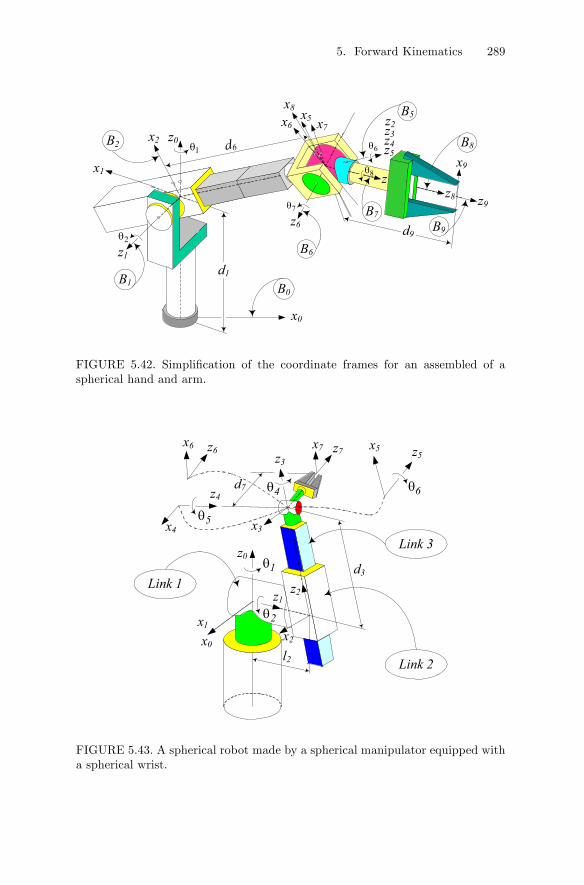
number of frames, and simplify the matrix calculations. However, we mayprefer to keep them and simplify the assembling process of changing thewrist with a new one. If this assembled robot is supposed to work for a while,we may do the elimination and simplify the robot to the one in Figure 5.42.We should mathematically substitute the eliminated frames B3 and B4 bya transformation matrix 2T5.
2T5 = 2T33T4
4T5 =
⎡⎢⎢⎣1 0 0 00 1 0 00 0 1 d60 0 0 1
⎤⎥⎥⎦ (5.150)
d6 = d3 + d4 + d5 (5.151)
Now the forward kinematics of the tool frame B9 becomes:
0T9 =0T1
1T22T5
5T66T7
7T88T9 (5.152)
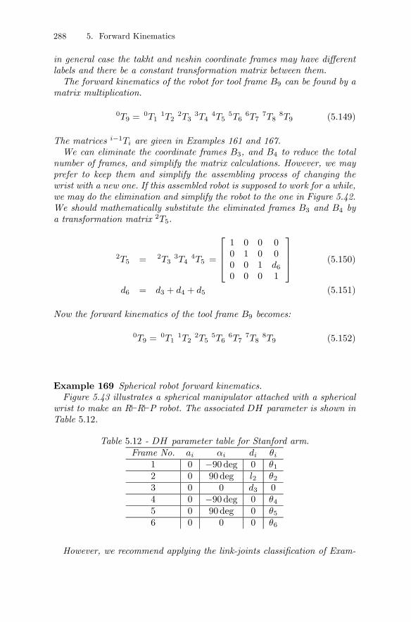
Example 169 Spherical robot forward kinematics.Figure 5.43 illustrates a spherical manipulator attached with a spherical
wrist to make an R`R`P robot. The associated DH parameter is shown inTable 5.12.
Table 5.12 - DH parameter table for Stanford arm.Frame No. ai αi di θi
1 0 −90 deg 0 θ12 0 90 deg l2 θ23 0 0 d3 04 0 −90 deg 0 θ45 0 90 deg 0 θ56 0 0 0 θ6
However, we recommend applying the link-joints classification of Exam-
5. Forward Kinematics 289
z6
7θ
z5
x6
z9
x9
6θ
x7
z8
B5
B6
B8
8θ
x8 x5
z7
d6
B7B9
x0
z0
z1
2θ
x1
1θ
z2x2
z3
B0B1
z4B2
d1
d9
FIGURE 5.42. Simplification of the coordinate frames for an assembled of aspherical hand and arm.
l2
z2
d3
z1
z0
d7
z3
z4
z5z7
x2
x1
x0
x3x4
x5x7z6x6
Link 1
Link 2
Link 3
2θ
1θ
5θ
4θ 6θ
FIGURE 5.43. A spherical robot made by a spherical manipulator equipped witha spherical wrist.

290 5. Forward Kinematics
ples 142 to 147. The link-joint combinations are shown in Table 5.13.
Table 5.13 - DH parameter table for setting up the link frames.Link No. Type
1 R`R(−90)2 R`P(90)3 PkR(0)4 R`R(−90)5 R`R(90)6 RkR(0)
Employing the associated transformation matrices for moving from Bi toBi−1 shows that
0T1 =
⎡⎢⎢⎣cos θ1 0 − sin θ1 0sin θ1 0 cos θ1 00 −1 0 00 0 0 1
⎤⎥⎥⎦ (5.153)
1T2 =
⎡⎢⎢⎣cos θ2 0 sin θ2 0sin θ2 0 − cos θ2 00 1 0 l20 0 0 1
⎤⎥⎥⎦ (5.154)
2T3 =
⎡⎢⎢⎣1 0 0 00 1 0 00 0 1 d30 0 0 1
⎤⎥⎥⎦ (5.155)
3T4 =
⎡⎢⎢⎣cos θ4 0 − sin θ4 0sin θ4 0 cos θ4 00 −1 0 00 0 0 1
⎤⎥⎥⎦ (5.156)
4T5 =
⎡⎢⎢⎣cos θ5 0 sin θ5 0sin θ5 0 − cos θ5 00 1 0 00 0 0 1
⎤⎥⎥⎦ (5.157)
5T6 =
⎡⎢⎢⎣cos θ6 − sin θ6 0 0sin θ6 cos θ6 0 00 0 1 00 0 0 1
⎤⎥⎥⎦ . (5.158)
Therefore, the configuration of the wrist final coordinate frame B6 in the
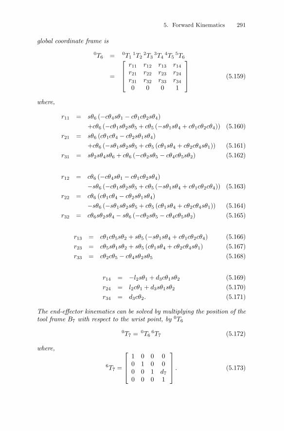
5. Forward Kinematics 291
global coordinate frame is
0T6 = 0T11T2
2T33T4
4T55T6
=
⎡⎢⎢⎣r11 r12 r13 r14r21 r22 r23 r24r31 r32 r33 r340 0 0 1
⎤⎥⎥⎦ (5.159)
where,
r11 = sθ6 (−cθ4sθ1 − cθ1cθ2sθ4)
+cθ6 (−cθ1sθ2sθ5 + cθ5 (−sθ1sθ4 + cθ1cθ2cθ4)) (5.160)
r21 = sθ6 (cθ1cθ4 − cθ2sθ1sθ4)
+cθ6 (−sθ1sθ2sθ5 + cθ5 (cθ1sθ4 + cθ2cθ4sθ1)) (5.161)
r31 = sθ2sθ4sθ6 + cθ6 (−cθ2sθ5 − cθ4cθ5sθ2) (5.162)
r12 = cθ6 (−cθ4sθ1 − cθ1cθ2sθ4)
−sθ6 (−cθ1sθ2sθ5 + cθ5 (−sθ1sθ4 + cθ1cθ2cθ4)) (5.163)
r22 = cθ6 (cθ1cθ4 − cθ2sθ1sθ4)
−sθ6 (−sθ1sθ2sθ5 + cθ5 (cθ1sθ4 + cθ2cθ4sθ1)) (5.164)
r32 = cθ6sθ2sθ4 − sθ6 (−cθ2sθ5 − cθ4cθ5sθ2) (5.165)
r13 = cθ1cθ5sθ2 + sθ5 (−sθ1sθ4 + cθ1cθ2cθ4) (5.166)
r23 = cθ5sθ1sθ2 + sθ5 (cθ1sθ4 + cθ2cθ4sθ1) (5.167)
r33 = cθ2cθ5 − cθ4sθ2sθ5 (5.168)
r14 = −l2sθ1 + d3cθ1sθ2 (5.169)
r24 = l2cθ1 + d3sθ1sθ2 (5.170)
r34 = d3cθ2. (5.171)
The end-effector kinematics can be solved by multiplying the position of thetool frame B7 with respect to the wrist point, by 0T6
0T7 =0T6
6T7 (5.172)
where,
6T7 =
⎡⎢⎢⎣1 0 0 00 1 0 00 0 1 d70 0 0 1
⎤⎥⎥⎦ . (5.173)
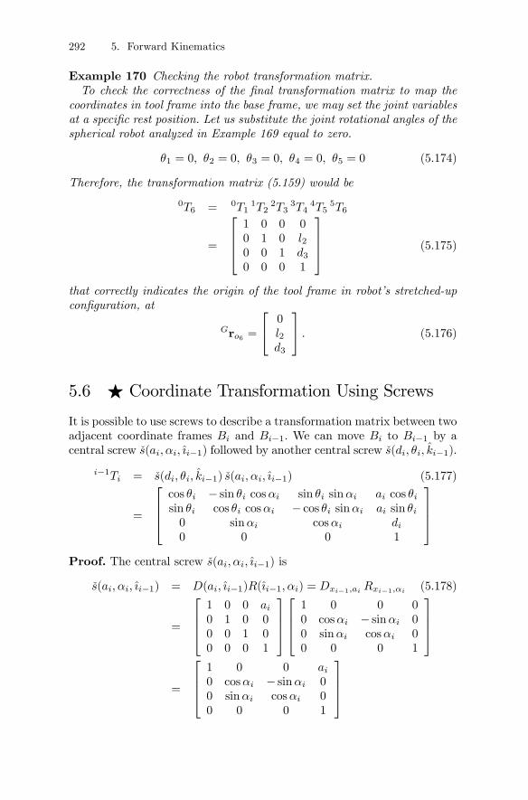
292 5. Forward Kinematics
Example 170 Checking the robot transformation matrix.To check the correctness of the final transformation matrix to map the
coordinates in tool frame into the base frame, we may set the joint variablesat a specific rest position. Let us substitute the joint rotational angles of thespherical robot analyzed in Example 169 equal to zero.
θ1 = 0, θ2 = 0, θ3 = 0, θ4 = 0, θ5 = 0 (5.174)
Therefore, the transformation matrix (5.159) would be
0T6 = 0T11T2
2T33T4
4T55T6
=
⎡⎢⎢⎣1 0 0 00 1 0 l20 0 1 d30 0 0 1
⎤⎥⎥⎦ (5.175)
that correctly indicates the origin of the tool frame in robot’s stretched-upconfiguration, at
Gro6 =
⎡⎣ 0l2d3
⎤⎦ . (5.176)
5.6 F Coordinate Transformation Using Screws
It is possible to use screws to describe a transformation matrix between twoadjacent coordinate frames Bi and Bi−1. We can move Bi to Bi−1 by acentral screw s(ai, αi, ıi−1) followed by another central screw s(di, θi, ki−1).
i−1Ti = s(di, θi, ki−1) s(ai, αi, ıi−1) (5.177)
=
⎡⎢⎢⎣cos θi − sin θi cosαi sin θi sinαi ai cos θisin θi cos θi cosαi − cos θi sinαi ai sin θi0 sinαi cosαi di0 0 0 1
⎤⎥⎥⎦Proof. The central screw s(ai, αi, ıi−1) is
s(ai, αi, ıi−1) = D(ai, ıi−1)R(ıi−1, αi) = Dxi−1,ai Rxi−1,αi (5.178)
=
⎡⎢⎢⎣1 0 0 ai0 1 0 00 0 1 00 0 0 1
⎤⎥⎥⎦⎡⎢⎢⎣1 0 0 00 cosαi − sinαi 00 sinαi cosαi 00 0 0 1
⎤⎥⎥⎦
=
⎡⎢⎢⎣1 0 0 ai0 cosαi − sinαi 00 sinαi cosαi 00 0 0 1
⎤⎥⎥⎦
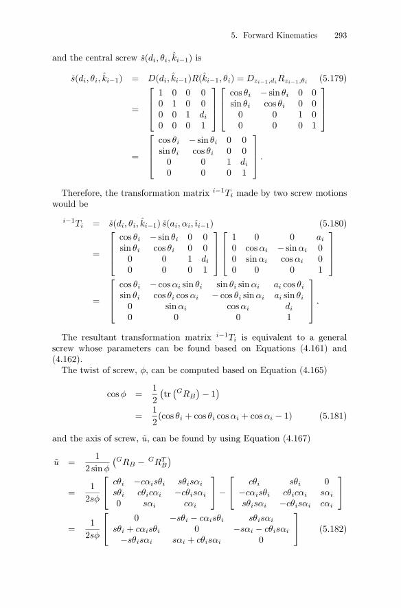
5. Forward Kinematics 293
and the central screw s(di, θi, ki−1) is
s(di, θi, ki−1) = D(di, ki−1)R(ki−1, θi) = Dzi−1,diRzi−1,θi (5.179)
=
⎡⎢⎢⎣1 0 0 00 1 0 00 0 1 di0 0 0 1
⎤⎥⎥⎦⎡⎢⎢⎣cos θi − sin θi 0 0sin θi cos θi 0 00 0 1 00 0 0 1
⎤⎥⎥⎦
=
⎡⎢⎢⎣cos θi − sin θi 0 0sin θi cos θi 0 00 0 1 di0 0 0 1
⎤⎥⎥⎦ .Therefore, the transformation matrix i−1Ti made by two screw motions
would be
i−1Ti = s(di, θi, ki−1) s(ai, αi, ıi−1) (5.180)
=
⎡⎢⎢⎣cos θi − sin θi 0 0sin θi cos θi 0 00 0 1 di0 0 0 1
⎤⎥⎥⎦⎡⎢⎢⎣1 0 0 ai0 cosαi − sinαi 00 sinαi cosαi 00 0 0 1
⎤⎥⎥⎦
=
⎡⎢⎢⎣cos θi − cosαi sin θi sin θi sinαi ai cos θisin θi cos θi cosαi − cos θi sinαi ai sin θi0 sinαi cosαi di0 0 0 1
⎤⎥⎥⎦ .The resultant transformation matrix i−1Ti is equivalent to a general
screw whose parameters can be found based on Equations (4.161) and(4.162).The twist of screw, φ, can be computed based on Equation (4.165)
cosφ =1
2
¡tr¡GRB
¢− 1¢
=1
2(cos θi + cos θi cosαi + cosαi − 1) (5.181)
and the axis of screw, u, can be found by using Equation (4.167)
u =1
2 sinφ
¡GRB − GRT
B
¢=
1
2sφ
⎡⎣ cθi −cαisθi sθisαisθi cθicαi −cθisαi0 sαi cαi
⎤⎦−⎡⎣ cθi sθi 0−cαisθi cθicαi sαisθisαi −cθisαi cαi
⎤⎦=
1
2sφ
⎡⎣ 0 −sθi − cαisθi sθisαisθi + cαisθi 0 −sαi − cθisαi−sθisαi sαi + cθisαi 0
⎤⎦ (5.182)
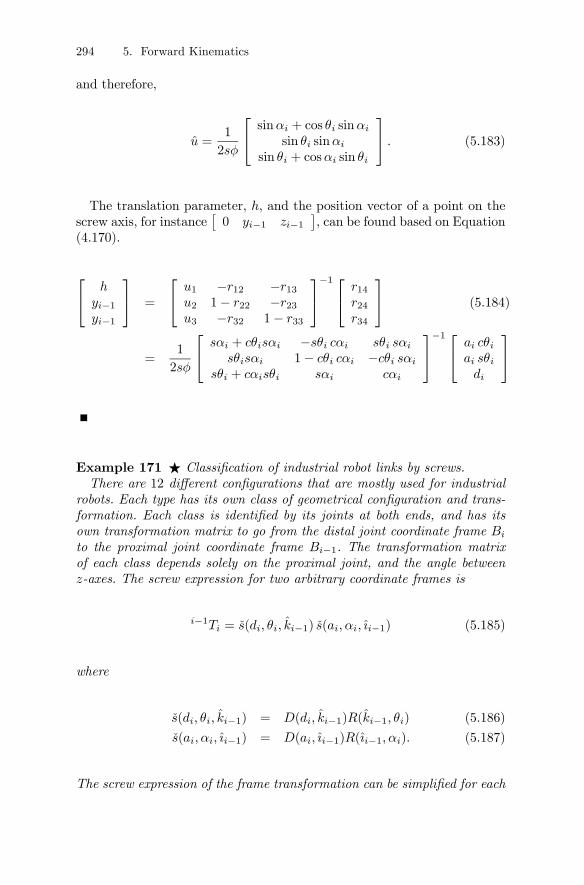
294 5. Forward Kinematics
and therefore,
u =1
2sφ
⎡⎣ sinαi + cos θi sinαisin θi sinαi
sin θi + cosαi sin θi
⎤⎦ . (5.183)
The translation parameter, h, and the position vector of a point on thescrew axis, for instance
£0 yi−1 zi−1
¤, can be found based on Equation
(4.170).
⎡⎣ hyi−1yi−1
⎤⎦ =
⎡⎣ u1 −r12 −r13u2 1− r22 −r23u3 −r32 1− r33
⎤⎦−1 ⎡⎣ r14r24r34
⎤⎦ (5.184)
=1
2sφ
⎡⎣ sαi + cθisαi −sθi cαi sθi sαisθisαi 1− cθi cαi −cθi sαi
sθi + cαisθi sαi cαi
⎤⎦−1 ⎡⎣ ai cθiai sθidi
⎤⎦
Example 171 F Classification of industrial robot links by screws.There are 12 different configurations that are mostly used for industrial
robots. Each type has its own class of geometrical configuration and trans-formation. Each class is identified by its joints at both ends, and has itsown transformation matrix to go from the distal joint coordinate frame Bi
to the proximal joint coordinate frame Bi−1. The transformation matrixof each class depends solely on the proximal joint, and the angle betweenz-axes. The screw expression for two arbitrary coordinate frames is
i−1Ti = s(di, θi, ki−1) s(ai, αi, ıi−1) (5.185)
where
s(di, θi, ki−1) = D(di, ki−1)R(ki−1, θi) (5.186)
s(ai, αi, ıi−1) = D(ai, ıi−1)R(ıi−1, αi). (5.187)
The screw expression of the frame transformation can be simplified for each
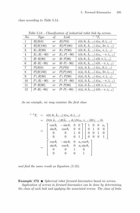
5. Forward Kinematics 295
class according to Table 5.14.
Table 5.14 - Classification of industrial robot link by screws.No. Type of Link i−1Ti1 RkR(0) or RkP(0) s(0, θi, ki−1) s(ai, 0, ıi−1)
2 RkR(180) or RkP(180) s(0, θi, ki−1) s(ai, 2π, ıi−1)
3 R⊥R(90) or R⊥P(90) s(0, θi, ki−1) s(ai, π, ıi−1)
4 R⊥R(−90) or R⊥P(−90) s(0, θi, ki−1) s(ai,−π, ıi−1)5 R`R(90) or R`P(90) s(0, θi, ki−1) s(0, π, ıi−1)
6 R`R(−90) or R`P(−90) s(0, θi, ki−1) s(0,−π, ıi−1)7 PkR(0) or PkP(0) s(di, 0, ki−1) s(ai, 0, ıi−1)
8 PkR(180) or PkP(180) s(di, 0, ki−1) s(ai, 2π, ıi−1)
9 P⊥R(90) or P⊥P(90) s(di, 0, ki−1) s(ai, π, ıi−1)
10 P⊥R(−90) or P⊥P(−90) s(di, 0, ki−1) s(ai,−π, ıi−1)11 P`R(90) or P`P(90) s(di, 0, ki−1) s(0, π, ıi−1)
12 P`R(−90) or P`P(−90) s(di, 0, ki−1) s(0,−π, ıi−1)
As an example, we may examine the first class
i−1Ti = s(0, θi, ki−1) s(ai, 0, ıi−1)
= D(0, ki−1)R(ki−1, θi)D(ai, ıi−1)R(ıi−1, 0)
=
⎡⎢⎢⎣cos θi − sin θi 0 0sin θi cos θi 0 00 0 1 00 0 0 1
⎤⎥⎥⎦⎡⎢⎢⎣1 0 0 ai0 1 0 00 0 1 00 0 0 1
⎤⎥⎥⎦
=
⎡⎢⎢⎣cos θi − sin θi 0 ai cos θisin θi cos θi 0 ai sin θi0 0 1 00 0 0 1
⎤⎥⎥⎦
and find the same result as Equation (5.32).
Example 172 F Spherical robot forward kinematics based on screws.Application of screws in forward kinematics can be done by determining
the class of each link and applying the associated screws. The class of links
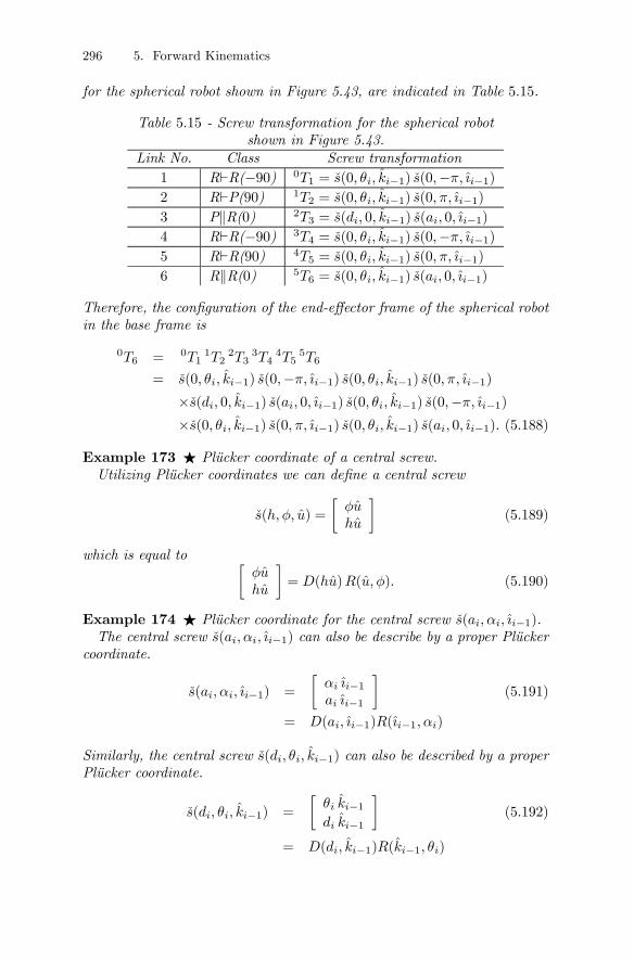
296 5. Forward Kinematics
for the spherical robot shown in Figure 5.43, are indicated in Table 5.15.
Table 5.15 - Screw transformation for the spherical robotshown in Figure 5.43.
Link No. Class Screw transformation1 R`R(−90) 0T1 = s(0, θi, ki−1) s(0,−π, ıi−1)2 R`P(90) 1T2 = s(0, θi, ki−1) s(0, π, ıi−1)
3 PkR(0) 2T3 = s(di, 0, ki−1) s(ai, 0, ıi−1)
4 R`R(−90) 3T4 = s(0, θi, ki−1) s(0,−π, ıi−1)5 R`R(90) 4T5 = s(0, θi, ki−1) s(0, π, ıi−1)
6 RkR(0) 5T6 = s(0, θi, ki−1) s(ai, 0, ıi−1)
Therefore, the configuration of the end-effector frame of the spherical robotin the base frame is
0T6 = 0T11T2
2T33T4
4T55T6
= s(0, θi, ki−1) s(0,−π, ıi−1) s(0, θi, ki−1) s(0, π, ıi−1)×s(di, 0, ki−1) s(ai, 0, ıi−1) s(0, θi, ki−1) s(0,−π, ıi−1)×s(0, θi, ki−1) s(0, π, ıi−1) s(0, θi, ki−1) s(ai, 0, ıi−1). (5.188)
Example 173 F Plücker coordinate of a central screw.Utilizing Plücker coordinates we can define a central screw
s(h, φ, u) =
∙φuhu
¸(5.189)
which is equal to ∙φuhu
¸= D(hu)R(u, φ). (5.190)
Example 174 F Plücker coordinate for the central screw s(ai, αi, ıi−1).The central screw s(ai, αi, ıi−1) can also be describe by a proper Plücker
coordinate.
s(ai, αi, ıi−1) =
∙αi ıi−1ai ıi−1
¸(5.191)
= D(ai, ıi−1)R(ıi−1, αi)
Similarly, the central screw s(di, θi, ki−1) can also be described by a properPlücker coordinate.
s(di, θi, ki−1) =
∙θi ki−1di ki−1
¸(5.192)
= D(di, ki−1)R(ki−1, θi)
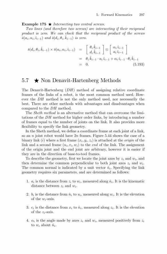
5. Forward Kinematics 297
Example 175 F Intersecting two central screws.Two lines (and therefore two screws) are intersecting if their reciprocal
product is zero. We can check that the reciprocal product of the screwss(ai, αi, ıi−1) and s(di, θi, ki−1) is zero.
s(di, θi, ki−1)× s(ai, αi, ıi−1) =
∙θi ki−1di ki−1
¸⊗∙αi ıi−1ai ıi−1
¸= θi ki−1 · ai ıi−1 + αi ıi−1 · θi ki−1= 0. (5.193)
5.7 F Non Denavit-Hartenberg Methods
The Denavit-Hartenberg (DH) method of assigning relative coordinateframes of the links of a robot, is the most common method used. How-ever the DH method is not the only method used, nor necessarily thebest. There are other methods with advantages and disadvantages whencompared to the DH method.The Sheth method is an alternative method that can overcome the limi-
tations of the DH method for higher order links, by introducing a numberof frames equal to the number of joints on the link. It also provides moreflexibility to specify the link geometry.In the Sheth method, we define a coordinate frame at each joint of a link,
so an n joint robot would have 2n frames. Figure 5.44 shows the case of abinary link (i) where a first frame (xi, yi, zi) is attached at the origin of thelink and a second frame (ui, vi, wi) to the end of the link. The assignmentof the origin joint and the end joint are arbitrary, however it is easier ifthey are in the direction of base-to-tool frames.To describe the geometry, first we locate the joint axes by zi and wi, and
then determine the common perpendicular to both joint axes zi and wi.The common normal is indicated by a unit vector ni. Specifying the linkgeometry requires six parameters, and are determined as follows:
1. ai is the distance from zi to wi, measured along ni. It is the kinematicdistance between zi and wi.
2. bi is the distance from ni to ui, measured along wi. It is the elevationof the wi-axis.
3. ci is the distance from xi to ni, measured along zi. It is the elevationof the zi-axis.
4. αi is the angle made by axes zi and wi, measured positively from zito wi about ni.
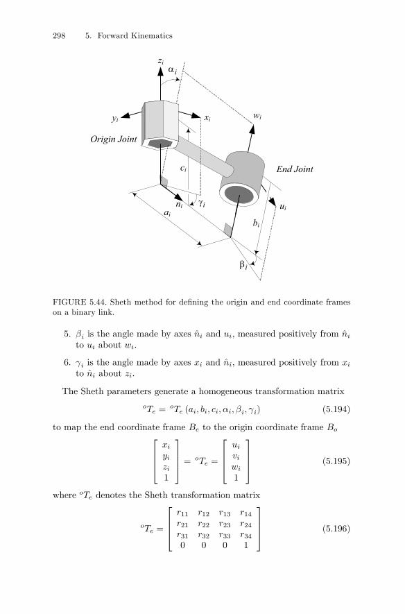
298 5. Forward Kinematics
xi
End Joint
Origin Joint
wi
bi
ni ui
yi
ai
ci
ziiα
iγ
iβ
FIGURE 5.44. Sheth method for defining the origin and end coordinate frameson a binary link.
5. βi is the angle made by axes ni and ui, measured positively from nito ui about wi.
6. γi is the angle made by axes xi and ni, measured positively from xito ni about zi.
The Sheth parameters generate a homogeneous transformation matrix
oTe =oTe (ai, bi, ci, αi, βi, γi) (5.194)
to map the end coordinate frame Be to the origin coordinate frame Bo⎡⎢⎢⎣xiyizi1
⎤⎥⎥⎦ = oTe =
⎡⎢⎢⎣uiviwi
1
⎤⎥⎥⎦ (5.195)
where oTe denotes the Sheth transformation matrix
oTe =
⎡⎢⎢⎣r11 r12 r13 r14r21 r22 r23 r24r31 r32 r33 r340 0 0 1
⎤⎥⎥⎦ (5.196)
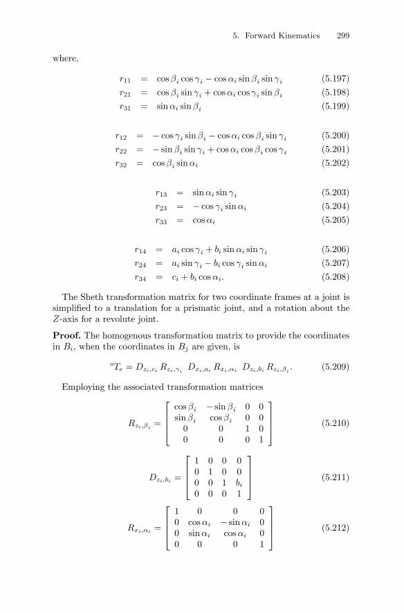
5. Forward Kinematics 299
where,
r11 = cosβi cos γi − cosαi sinβi sin γi (5.197)
r21 = cosβi sin γi + cosαi cos γi sinβi (5.198)
r31 = sinαi sinβi (5.199)
r12 = − cos γi sinβi − cosαi cosβi sin γi (5.200)
r22 = − sinβi sin γi + cosαi cosβi cos γi (5.201)
r32 = cosβi sinαi (5.202)
r13 = sinαi sin γi (5.203)
r23 = − cos γi sinαi (5.204)
r33 = cosαi (5.205)
r14 = ai cos γi + bi sinαi sin γi (5.206)
r24 = ai sin γi − bi cos γi sinαi (5.207)
r34 = ci + bi cosαi. (5.208)
The Sheth transformation matrix for two coordinate frames at a joint issimplified to a translation for a prismatic joint, and a rotation about theZ-axis for a revolute joint.
Proof. The homogenous transformation matrix to provide the coordinatesin Bi, when the coordinates in Bj are given, is
oTe = Dzi,ci Rzi,γi Dxi,ai Rxi,αi Dzi,bi Rzi,βi . (5.209)
Employing the associated transformation matrices
Rzi,βi =
⎡⎢⎢⎣cosβi − sinβi 0 0sinβi cosβi 0 00 0 1 00 0 0 1
⎤⎥⎥⎦ (5.210)
Dzi,bi =
⎡⎢⎢⎣1 0 0 00 1 0 00 0 1 bi0 0 0 1
⎤⎥⎥⎦ (5.211)
Rxi,αi =
⎡⎢⎢⎣1 0 0 00 cosαi − sinαi 00 sinαi cosαi 00 0 0 1
⎤⎥⎥⎦ (5.212)
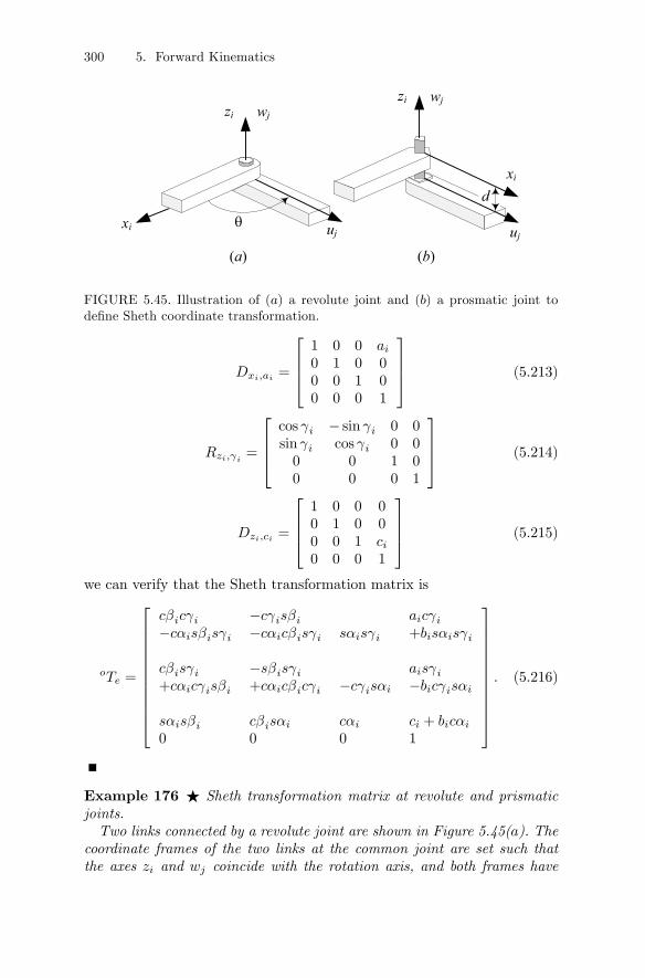
300 5. Forward Kinematics
xi
wjzi
wjzi
ujuj
xi
(a) (b)
θ
d
FIGURE 5.45. Illustration of (a) a revolute joint and (b) a prosmatic joint todefine Sheth coordinate transformation.
Dxi,ai =
⎡⎢⎢⎣1 0 0 ai0 1 0 00 0 1 00 0 0 1
⎤⎥⎥⎦ (5.213)
Rzi,γi =
⎡⎢⎢⎣cos γi − sin γi 0 0sin γi cos γi 0 00 0 1 00 0 0 1
⎤⎥⎥⎦ (5.214)
Dzi,ci =
⎡⎢⎢⎣1 0 0 00 1 0 00 0 1 ci0 0 0 1
⎤⎥⎥⎦ (5.215)
we can verify that the Sheth transformation matrix is
oTe =
⎡⎢⎢⎢⎢⎢⎢⎢⎢⎢⎢⎣
cβicγi −cγisβi aicγi−cαisβisγi −cαicβisγi sαisγi +bisαisγi
cβisγi −sβisγi aisγi+cαicγisβi +cαicβicγi −cγisαi −bicγisαi
sαisβi cβisαi cαi ci + bicαi0 0 0 1
⎤⎥⎥⎥⎥⎥⎥⎥⎥⎥⎥⎦. (5.216)
Example 176 F Sheth transformation matrix at revolute and prismaticjoints.Two links connected by a revolute joint are shown in Figure 5.45(a). The
coordinate frames of the two links at the common joint are set such thatthe axes zi and wj coincide with the rotation axis, and both frames have
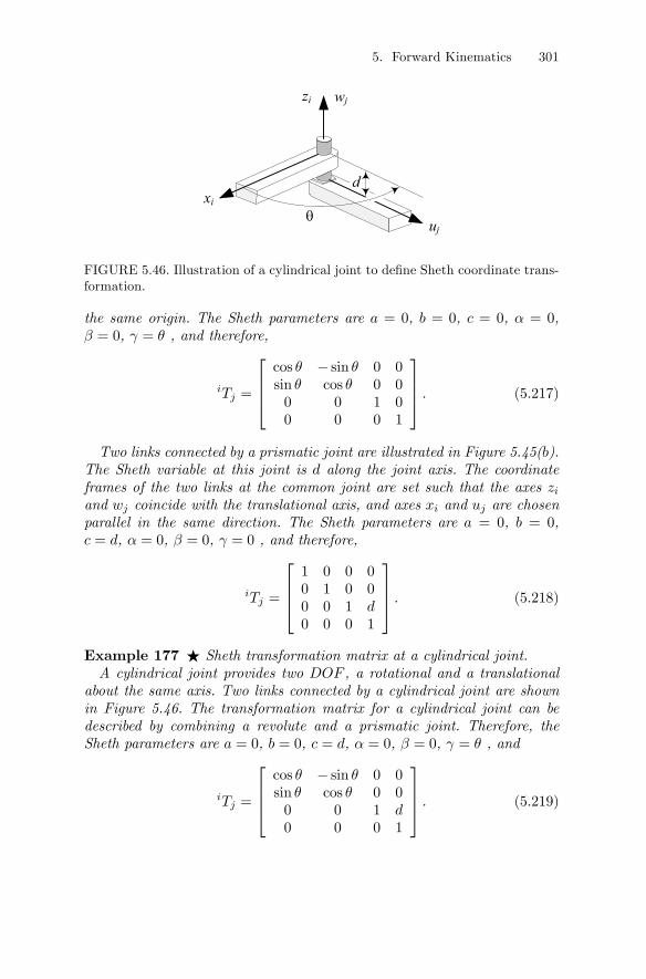
5. Forward Kinematics 301
wjzi
xiθ
d
uj
FIGURE 5.46. Illustration of a cylindrical joint to define Sheth coordinate trans-formation.
the same origin. The Sheth parameters are a = 0, b = 0, c = 0, α = 0,β = 0, γ = θ , and therefore,
iTj =
⎡⎢⎢⎣cos θ − sin θ 0 0sin θ cos θ 0 00 0 1 00 0 0 1
⎤⎥⎥⎦ . (5.217)
Two links connected by a prismatic joint are illustrated in Figure 5.45(b).The Sheth variable at this joint is d along the joint axis. The coordinateframes of the two links at the common joint are set such that the axes ziand wj coincide with the translational axis, and axes xi and uj are chosenparallel in the same direction. The Sheth parameters are a = 0, b = 0,c = d, α = 0, β = 0, γ = 0 , and therefore,
iTj =
⎡⎢⎢⎣1 0 0 00 1 0 00 0 1 d0 0 0 1
⎤⎥⎥⎦ . (5.218)
Example 177 F Sheth transformation matrix at a cylindrical joint.A cylindrical joint provides two DOF , a rotational and a translational
about the same axis. Two links connected by a cylindrical joint are shownin Figure 5.46. The transformation matrix for a cylindrical joint can bedescribed by combining a revolute and a prismatic joint. Therefore, theSheth parameters are a = 0, b = 0, c = d, α = 0, β = 0, γ = θ , and
iTj =
⎡⎢⎢⎣cos θ − sin θ 0 0sin θ cos θ 0 00 0 1 d0 0 0 1
⎤⎥⎥⎦ . (5.219)
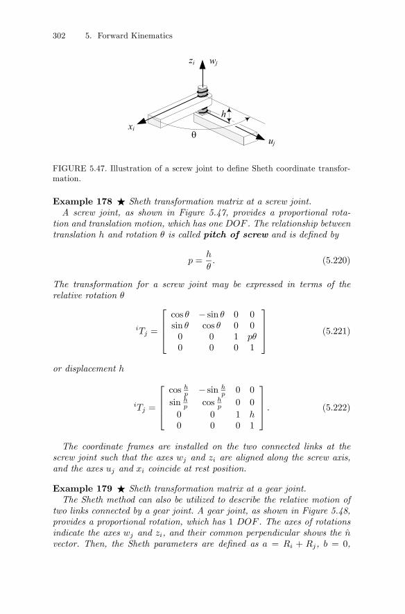
302 5. Forward Kinematics
wjzi
uj
xiθ
h
FIGURE 5.47. Illustration of a screw joint to define Sheth coordinate transfor-mation.
Example 178 F Sheth transformation matrix at a screw joint.A screw joint, as shown in Figure 5.47, provides a proportional rota-
tion and translation motion, which has one DOF . The relationship betweentranslation h and rotation θ is called pitch of screw and is defined by
p =h
θ. (5.220)
The transformation for a screw joint may be expressed in terms of therelative rotation θ
iTj =
⎡⎢⎢⎣cos θ − sin θ 0 0sin θ cos θ 0 00 0 1 pθ0 0 0 1
⎤⎥⎥⎦ (5.221)
or displacement h
iTj =
⎡⎢⎢⎣cos hp − sin h
p 0 0
sin hp cos hp 0 0
0 0 1 h0 0 0 1
⎤⎥⎥⎦ . (5.222)
The coordinate frames are installed on the two connected links at thescrew joint such that the axes wj and zi are aligned along the screw axis,and the axes uj and xi coincide at rest position.
Example 179 F Sheth transformation matrix at a gear joint.The Sheth method can also be utilized to describe the relative motion of
two links connected by a gear joint. A gear joint, as shown in Figure 5.48,provides a proportional rotation, which has 1 DOF . The axes of rotationsindicate the axes wj and zi, and their common perpendicular shows the nvector. Then, the Sheth parameters are defined as a = Ri + Rj, b = 0,
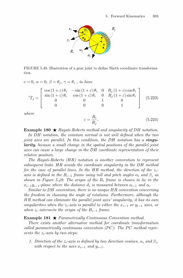
5. Forward Kinematics 303
zi
uj
xi
Ri
Rj
wj
n
iθ
FIGURE 5.48. Illustration of a gear joint to define Sheth coordinate transforma-tion.
c = 0, α = 0, β = θj, γ = θi , to have
iTj =
⎡⎢⎢⎣cos (1 + ε) θi − sin (1 + ε) θi 0 Rj (1 + ε) cos θisin (1 + ε) θi cos (1 + ε) θi 0 Rj (1 + ε) sin θi
0 0 1 00 0 0 1
⎤⎥⎥⎦ (5.223)
where
ε =Ri
Rj. (5.224)
Example 180 F Hayati-Roberts method and singularity of DH notation.In DH notation, the common normal is not well defined when the two
joint axes are parallel. In this condition, the DH notation has a singu-larity, because a small change in the spatial positions of the parallel jointaxes can cause a large change in the DH coordinate representation of theirrelative position.The Hayati-Roberts (HR) notation is another convention to represent
subsequent links. HR avoids the coordinate singularity in the DH methodfor the case of parallel lines. In the HR method, the direction of the zi-axis is defined in the Bi−1 frame using roll and pitch angles αi and βi asshown in Figure 5.49. The origin of the Bi frame is chosen to lie in thexi−1yi−1-plane where the distance di is measured between oi−1 and oi.Similar to DH convention, there is no unique HR convention concerning
the freedom in choosing the angle of rotations. Furthermore, although theHR method can eliminate the parallel joint axes’ singularity, it has its ownsingularities when the zi-axis is parallel to either the xi−1 or yi−1 axes, orwhen zi intersects the origin of the Bi−1 frame.
Example 181 F Parametrically Continuous Convention method.There exists another alternative method for coordinate transformation
called parametrically continuous convention (PC). The PC method repre-sents the zi-axis by two steps:
1. Direction of the zi-axis is defined by two direction cosines, αi and βi,with respect to the axes xi−1 and yi−1.
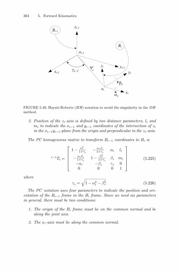
304 5. Forward Kinematics
xi-1
yi-1
zi-1
xi
yi
zi
oi-1
oid
i-1
Bi
Bi-1
i 1−γ
iα
iβ
FIGURE 5.49. Hayati-Roberts (HR) notation to avoid the singularity in the DHmethod.
2. Position of the zi-axis is defined by two distance parameters, li andmi to indicate the xi−1 and yi−1 coordinates of the intersection of ziin the xi−1yi−1-plane from the origin and perpendicular to the zi-axis.
The PC homogeneous matrix to transform Bi−1 coordinates to Bi is
i−1Ti =
⎡⎢⎢⎢⎢⎣1− α2i
1+γi− αiβi1+γi
αi li
− αiβi1+γi
1− β2i1+γi
βi mi
−αi −βi γi 00 0 0 1
⎤⎥⎥⎥⎥⎦ (5.225)
where
γi =
q1− α2i − β2i . (5.226)
The PC notation uses four parameters to indicate the position and ori-entation of the Bi−1 frame in the Bi frame. Since we need six parametersin general, there must be two conditions:
1. The origin of the Bi frame must lie on the common normal and bealong the joint axis.
2. The xi-axis must lie along the common normal.
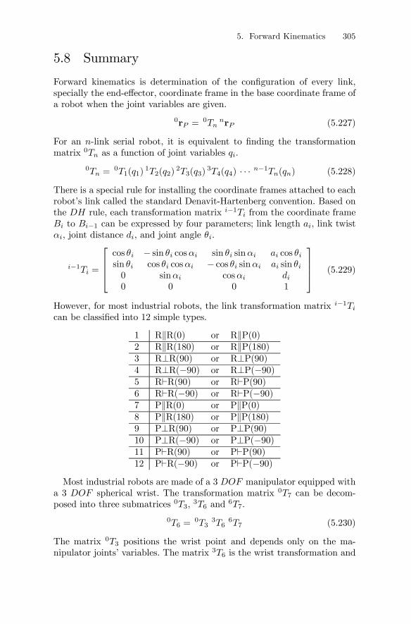
5. Forward Kinematics 305
5.8 Summary
Forward kinematics is determination of the configuration of every link,specially the end-effector, coordinate frame in the base coordinate frame ofa robot when the joint variables are given.
0rP =0Tn
nrP (5.227)
For an n-link serial robot, it is equivalent to finding the transformationmatrix 0Tn as a function of joint variables qi.
0Tn =0T1(q1)
1T2(q2)2T3(q3)
3T4(q4) · · · n−1Tn(qn) (5.228)
There is a special rule for installing the coordinate frames attached to eachrobot’s link called the standard Denavit-Hartenberg convention. Based onthe DH rule, each transformation matrix i−1Ti from the coordinate frameBi to Bi−1 can be expressed by four parameters; link length ai, link twistαi, joint distance di, and joint angle θi.
i−1Ti =
⎡⎢⎢⎣cos θi − sin θi cosαi sin θi sinαi ai cos θisin θi cos θi cosαi − cos θi sinαi ai sin θi0 sinαi cosαi di0 0 0 1
⎤⎥⎥⎦ (5.229)
However, for most industrial robots, the link transformation matrix i−1Tican be classified into 12 simple types.
1 RkR(0) or RkP(0)2 RkR(180) or RkP(180)3 R⊥R(90) or R⊥P(90)4 R⊥R(−90) or R⊥P(−90)5 R`R(90) or R`P(90)6 R`R(−90) or R`P(−90)7 PkR(0) or PkP(0)8 PkR(180) or PkP(180)9 P⊥R(90) or P⊥P(90)10 P⊥R(−90) or P⊥P(−90)11 P`R(90) or P`P(90)12 P`R(−90) or P`P(−90)
Most industrial robots are made of a 3 DOF manipulator equipped witha 3 DOF spherical wrist. The transformation matrix 0T7 can be decom-posed into three submatrices 0T3, 3T6 and 6T7.
0T6 =0T3
3T66T7 (5.230)
The matrix 0T3 positions the wrist point and depends only on the ma-nipulator joints’ variables. The matrix 3T6 is the wrist transformation and
306 5. Forward Kinematics
depends only on the manipulator wrist’s variables. The constant matrix6T7 is the tools transformation matrix. Decomposing 0T7 into submatricesenables us to make the forward kinematics modular.
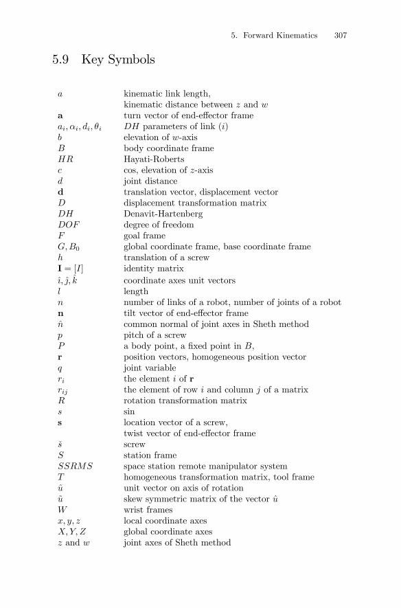
5. Forward Kinematics 307
5.9 Key Symbols
a kinematic link length,kinematic distance between z and w
a turn vector of end-effector frameai, αi, di, θi DH parameters of link (i)b elevation of w-axisB body coordinate frameHR Hayati-Robertsc cos, elevation of z-axisd joint distanced translation vector, displacement vectorD displacement transformation matrixDH Denavit-HartenbergDOF degree of freedomF goal frameG,B0 global coordinate frame, base coordinate frameh translation of a screwI = [I] identity matrixı, j, k coordinate axes unit vectorsl lengthn number of links of a robot, number of joints of a robotn tilt vector of end-effector framen common normal of joint axes in Sheth methodp pitch of a screwP a body point, a fixed point in B,r position vectors, homogeneous position vectorq joint variableri the element i of rrij the element of row i and column j of a matrixR rotation transformation matrixs sins location vector of a screw,
twist vector of end-effector frames screwS station frameSSRMS space station remote manipulator systemT homogeneous transformation matrix, tool frameu unit vector on axis of rotationu skew symmetric matrix of the vector uW wrist framesx, y, z local coordinate axesX,Y,Z global coordinate axesz and w joint axes of Sheth method
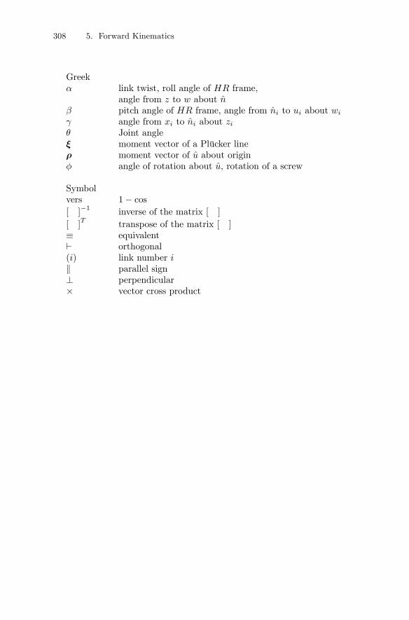
308 5. Forward Kinematics
Greekα link twist, roll angle of HR frame,
angle from z to w about nβ pitch angle of HR frame, angle from ni to ui about wi
γ angle from xi to ni about ziθ Joint angleξ moment vector of a Plücker lineρ moment vector of u about originφ angle of rotation about u, rotation of a screw
Symbolvers 1− cos[ ]−1 inverse of the matrix [ ]
[ ]T transpose of the matrix [ ]
≡ equivalent` orthogonal(i) link number ik parallel sign⊥ perpendicular× vector cross product
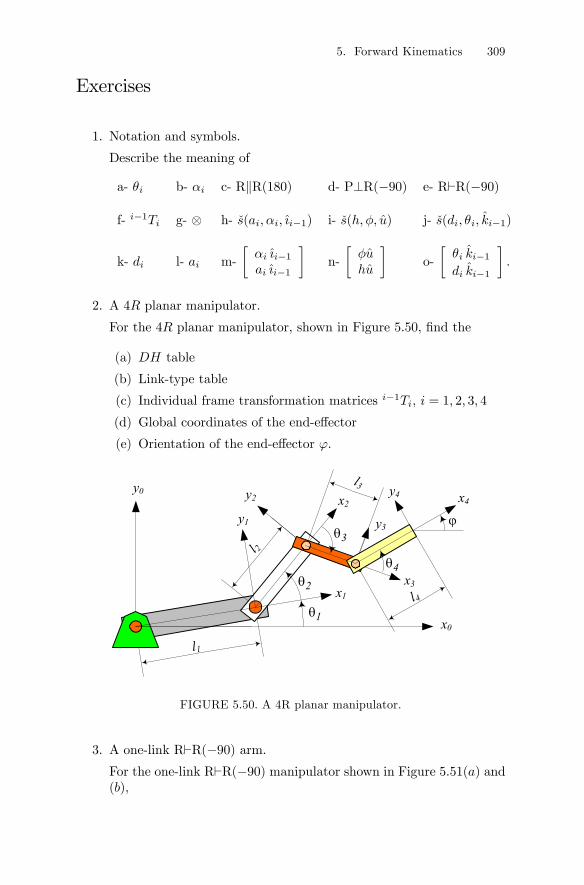
5. Forward Kinematics 309
Exercises
1. Notation and symbols.
Describe the meaning of
a- θi b- αi c- RkR(180) d- P⊥R(−90) e- R`R(−90)
f- i−1Ti g- ⊗ h- s(ai, αi, ıi−1) i- s(h, φ, u) j- s(di, θi, ki−1)
k- di l- ai m-∙αi ıi−1ai ıi−1
¸n-∙φuhu
¸o-∙θi ki−1di ki−1
¸.
2. A 4R planar manipulator.
For the 4R planar manipulator, shown in Figure 5.50, find the
(a) DH table
(b) Link-type table
(c) Individual frame transformation matrices i−1Ti, i = 1, 2, 3, 4
(d) Global coordinates of the end-effector
(e) Orientation of the end-effector ϕ.
x2y2
y0
y1
x1
y3
x0
x4y4
x3
1θ
2θ
l1
l 2
l3
l4
3θ
4θ
ϕ
FIGURE 5.50. A 4R planar manipulator.
3. A one-link R`R(−90) arm.For the one-link R`R(−90) manipulator shown in Figure 5.51(a) and(b),
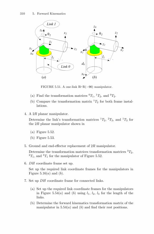
310 5. Forward Kinematics
1θ
l1
z1
z0
z2x1
x0
Link 1
Link 0
l1
z2
z1
z0
x2x1
x0
x2
d0
(a) (b)
1θ
FIGURE 5.51. A one-link R`R(−90) manipulator.
(a) Find the transformation matrices 0T1, 1T2, and 0T2.
(b) Compare the transformation matrix 1T2 for both frame instal-lations.
4. A 2R planar manipulator.
Determine the link’s transformation matrices 1T2, 2T3, and 1T3 forthe 2R planar manipulator shown in
(a) Figure 5.52.
(b) Figure 5.53.
5. Ground and end-effector replacement of 2R manipulator.
Determine the transformation matrices transformation matrices 3T2,2T1, and 3T1 for the manipulator of Figure 5.52.
6. DH coordinate frame set up.
Set up the required link coordinate frames for the manipulators inFigure 5.16(a) and (b).
7. Set up DH coordinate frame for connected links.
(a) Set up the required link coordinate frames for the manipulatorsin Figure 5.54(a) and (b) using l1, l2, l3 for the length of thelinks.
(b) Determine the forward kinematics transformation matrix of themanipulator in 5.54(a) and (b) and find their rest positions.
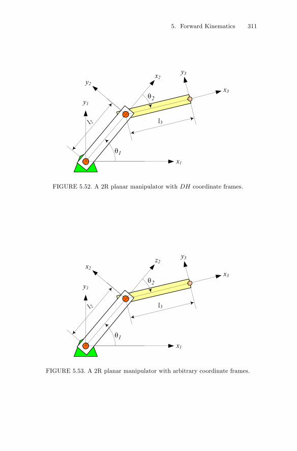
5. Forward Kinematics 311
x3
y3
y1
y2l 2
x2
x1
l3
1θ
2θ
FIGURE 5.52. A 2R planar manipulator with DH coordinate frames.
x3
y3
y1
x2
l 2
z2
x1
l3
1θ
2θ
FIGURE 5.53. A 2R planar manipulator with arbitrary coordinate frames.
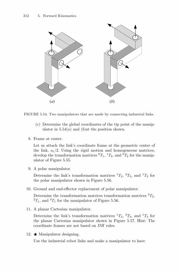
312 5. Forward Kinematics
(a) (b)
FIGURE 5.54. Two manipulators that are made by connecting industrial links.
(c) Determine the global coordinates of the tip point of the manip-ulator in 5.54(a) and (b)at the position shown.
8. Frame at center.
Let us attach the link’s coordinate frame at the geometric center ofthe link, ai/2. Using the rigid motion and homogeneous matrices,develop the transformation matrices 0T1, 1T2, and 0T2 for the manip-ulator of Figure 5.55.
9. A polar manipulator.
Determine the link’s transformation matrices 1T2, 2T3, and 1T3 forthe polar manipulator shown in Figure 5.56.
10. Ground and end-effector replacement of polar manipulator.
Determine the transformation matrices transformation matrices 3T2,2T1, and 3T1 for the manipulator of Figure 5.56.
11. A planar Cartesian manipulator.
Determine the link’s transformation matrices 1T2, 2T3, and 1T3 forthe planar Cartesian manipulator shown in Figure 5.57. Hint: Thecoordinate frames are not based on DH rules.
12. F Manipulator designing.
Use the industrial robot links and make a manipulator to have
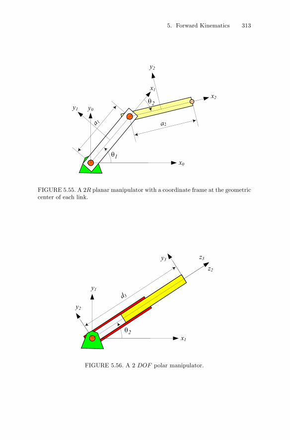
5. Forward Kinematics 313
x2
y2
y0
x1a 1
y1
x0
a2
1θ
2θ
FIGURE 5.55. A 2R planar manipulator with a coordinate frame at the geometriccenter of each link.
z2
y3
y1
y2
d3
z3
x12θ
FIGURE 5.56. A 2 DOF polar manipulator.
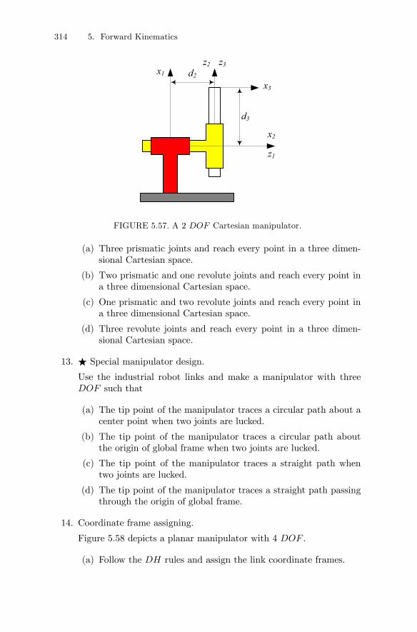
314 5. Forward Kinematics
z2
x3
x1
x2
z3
z1
d2
d3
FIGURE 5.57. A 2 DOF Cartesian manipulator.
(a) Three prismatic joints and reach every point in a three dimen-sional Cartesian space.
(b) Two prismatic and one revolute joints and reach every point ina three dimensional Cartesian space.
(c) One prismatic and two revolute joints and reach every point ina three dimensional Cartesian space.
(d) Three revolute joints and reach every point in a three dimen-sional Cartesian space.
13. F Special manipulator design.
Use the industrial robot links and make a manipulator with threeDOF such that
(a) The tip point of the manipulator traces a circular path about acenter point when two joints are lucked.
(b) The tip point of the manipulator traces a circular path aboutthe origin of global frame when two joints are lucked.
(c) The tip point of the manipulator traces a straight path whentwo joints are lucked.
(d) The tip point of the manipulator traces a straight path passingthrough the origin of global frame.
14. Coordinate frame assigning.
Figure 5.58 depicts a planar manipulator with 4 DOF .
(a) Follow the DH rules and assign the link coordinate frames.
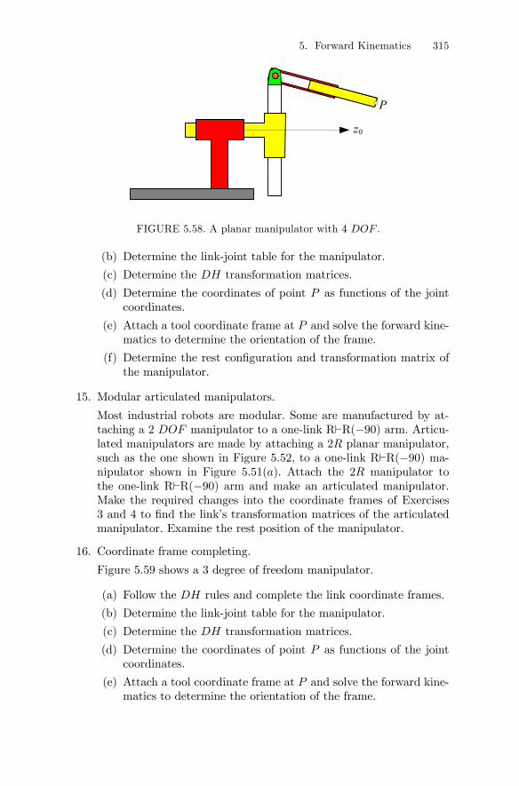
5. Forward Kinematics 315
z0
P
FIGURE 5.58. A planar manipulator with 4 DOF .
(b) Determine the link-joint table for the manipulator.
(c) Determine the DH transformation matrices.
(d) Determine the coordinates of point P as functions of the jointcoordinates.
(e) Attach a tool coordinate frame at P and solve the forward kine-matics to determine the orientation of the frame.
(f) Determine the rest configuration and transformation matrix ofthe manipulator.
15. Modular articulated manipulators.
Most industrial robots are modular. Some are manufactured by at-taching a 2 DOF manipulator to a one-link R`R(−90) arm. Articu-lated manipulators are made by attaching a 2R planar manipulator,such as the one shown in Figure 5.52, to a one-link R`R(−90) ma-nipulator shown in Figure 5.51(a). Attach the 2R manipulator tothe one-link R`R(−90) arm and make an articulated manipulator.Make the required changes into the coordinate frames of Exercises3 and 4 to find the link’s transformation matrices of the articulatedmanipulator. Examine the rest position of the manipulator.
16. Coordinate frame completing.
Figure 5.59 shows a 3 degree of freedom manipulator.
(a) Follow the DH rules and complete the link coordinate frames.
(b) Determine the link-joint table for the manipulator.
(c) Determine the DH transformation matrices.
(d) Determine the coordinates of point P as functions of the jointcoordinates.
(e) Attach a tool coordinate frame at P and solve the forward kine-matics to determine the orientation of the frame.
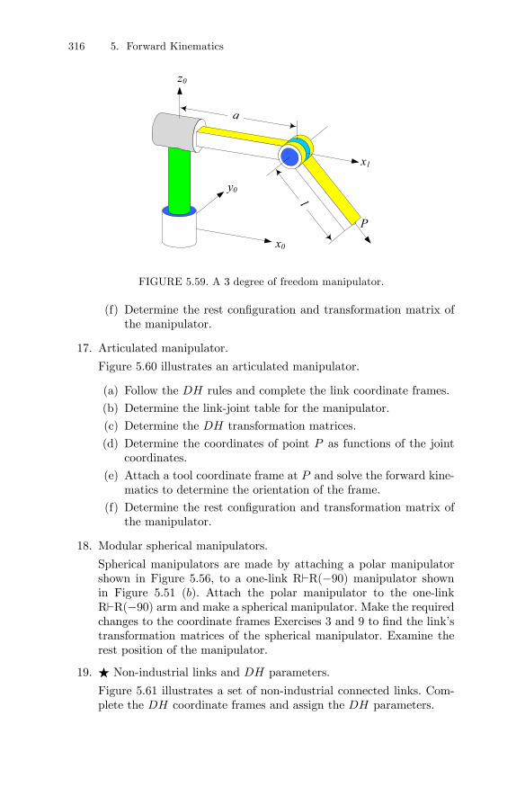
316 5. Forward Kinematics
x0
y0
x1
a
l
z0
P
FIGURE 5.59. A 3 degree of freedom manipulator.
(f) Determine the rest configuration and transformation matrix ofthe manipulator.
17. Articulated manipulator.
Figure 5.60 illustrates an articulated manipulator.
(a) Follow the DH rules and complete the link coordinate frames.
(b) Determine the link-joint table for the manipulator.
(c) Determine the DH transformation matrices.
(d) Determine the coordinates of point P as functions of the jointcoordinates.
(e) Attach a tool coordinate frame at P and solve the forward kine-matics to determine the orientation of the frame.
(f) Determine the rest configuration and transformation matrix ofthe manipulator.
18. Modular spherical manipulators.
Spherical manipulators are made by attaching a polar manipulatorshown in Figure 5.56, to a one-link R`R(−90) manipulator shownin Figure 5.51 (b). Attach the polar manipulator to the one-linkR`R(−90) arm and make a spherical manipulator. Make the requiredchanges to the coordinate frames Exercises 3 and 9 to find the link’stransformation matrices of the spherical manipulator. Examine therest position of the manipulator.
19. F Non-industrial links and DH parameters.
Figure 5.61 illustrates a set of non-industrial connected links. Com-plete the DH coordinate frames and assign the DH parameters.
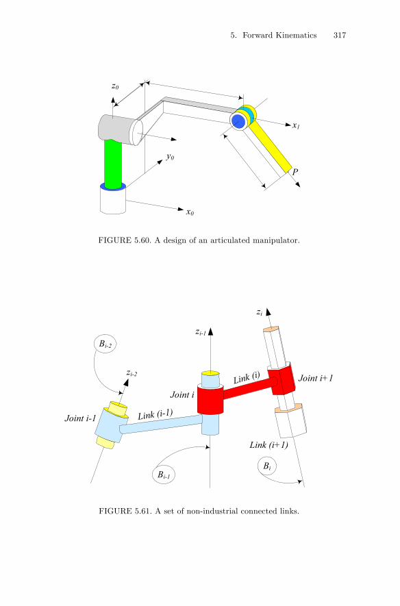
5. Forward Kinematics 317
x0
y0
x1
z0
P
FIGURE 5.60. A design of an articulated manipulator.
zi
Link (i)
Link (i+1)
Joint i-1
zi-2
Bi
Bi-2
Bi-1
Link (i-1)
Joint i
Joint i+1
zi-1
FIGURE 5.61. A set of non-industrial connected links.
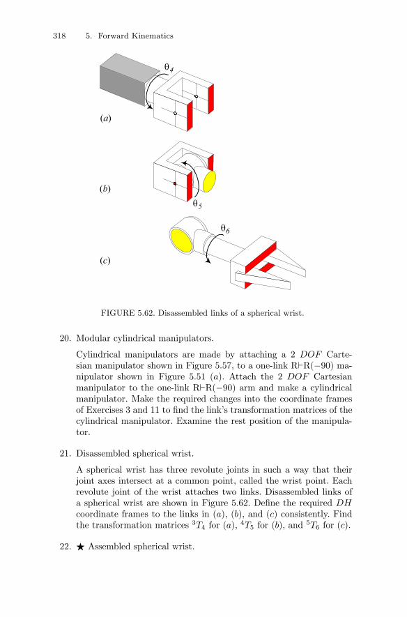
318 5. Forward Kinematics
(a)
(b)
(c)
4θ
5θ
6θ
FIGURE 5.62. Disassembled links of a spherical wrist.
20. Modular cylindrical manipulators.
Cylindrical manipulators are made by attaching a 2 DOF Carte-sian manipulator shown in Figure 5.57, to a one-link R`R(−90) ma-nipulator shown in Figure 5.51 (a). Attach the 2 DOF Cartesianmanipulator to the one-link R`R(−90) arm and make a cylindricalmanipulator. Make the required changes into the coordinate framesof Exercises 3 and 11 to find the link’s transformation matrices of thecylindrical manipulator. Examine the rest position of the manipula-tor.
21. Disassembled spherical wrist.
A spherical wrist has three revolute joints in such a way that theirjoint axes intersect at a common point, called the wrist point. Eachrevolute joint of the wrist attaches two links. Disassembled links ofa spherical wrist are shown in Figure 5.62. Define the required DHcoordinate frames to the links in (a), (b), and (c) consistently. Findthe transformation matrices 3T4 for (a), 4T5 for (b), and 5T6 for (c).
22. F Assembled spherical wrist.
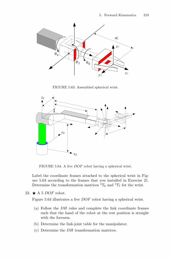
5. Forward Kinematics 319
z7
d7
x7
y7
4θ
5θ 6θ
FIGURE 5.63. Assembled spherical wrist.
x0
y0
z0
FIGURE 5.64. A five DOF robot having a spherical wrist.
Label the coordinate frames attached to the spherical wrist in Fig-ure 5.63 according to the frames that you installed in Exercise 21.Determine the transformation matrices 3T6 and 3T7 for the wrist.
23. F A 5 DOF robot.
Figure 5.64 illustrates a five DOF robot having a spherical wrist.
(a) Follow the DH rules and complete the link coordinate framessuch that the hand of the robot at the rest position is straightwith the forearm.
(b) Determine the link-joint table for the manipulator.
(c) Determine the DH transformation matrices.
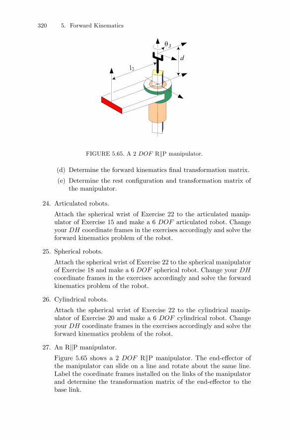
320 5. Forward Kinematics
dl2
3θ
FIGURE 5.65. A 2 DOF RkP manipulator.
(d) Determine the forward kinematics final transformation matrix.
(e) Determine the rest configuration and transformation matrix ofthe manipulator.
24. Articulated robots.
Attach the spherical wrist of Exercise 22 to the articulated manip-ulator of Exercise 15 and make a 6 DOF articulated robot. Changeyour DH coordinate frames in the exercises accordingly and solve theforward kinematics problem of the robot.
25. Spherical robots.
Attach the spherical wrist of Exercise 22 to the spherical manipulatorof Exercise 18 and make a 6 DOF spherical robot. Change your DHcoordinate frames in the exercises accordingly and solve the forwardkinematics problem of the robot.
26. Cylindrical robots.
Attach the spherical wrist of Exercise 22 to the cylindrical manip-ulator of Exercise 20 and make a 6 DOF cylindrical robot. Changeyour DH coordinate frames in the exercises accordingly and solve theforward kinematics problem of the robot.
27. An RkP manipulator.Figure 5.65 shows a 2 DOF RkP manipulator. The end-effector ofthe manipulator can slide on a line and rotate about the same line.Label the coordinate frames installed on the links of the manipulatorand determine the transformation matrix of the end-effector to thebase link.
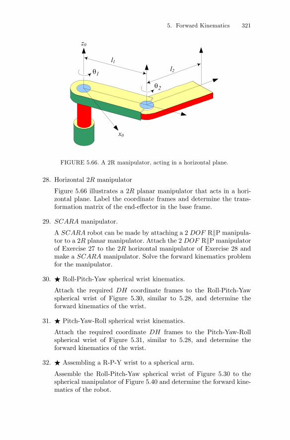
5. Forward Kinematics 321
z0
l1
x0
l21θ
2θ
FIGURE 5.66. A 2R manipulator, acting in a horizontal plane.
28. Horizontal 2R manipulator
Figure 5.66 illustrates a 2R planar manipulator that acts in a hori-zontal plane. Label the coordinate frames and determine the trans-formation matrix of the end-effector in the base frame.
29. SCARA manipulator.
A SCARA robot can be made by attaching a 2 DOF RkP manipula-tor to a 2R planar manipulator. Attach the 2 DOF RkP manipulatorof Exercise 27 to the 2R horizontal manipulator of Exercise 28 andmake a SCARA manipulator. Solve the forward kinematics problemfor the manipulator.
30. F Roll-Pitch-Yaw spherical wrist kinematics.
Attach the required DH coordinate frames to the Roll-Pitch-Yawspherical wrist of Figure 5.30, similar to 5.28, and determine theforward kinematics of the wrist.
31. F Pitch-Yaw-Roll spherical wrist kinematics.
Attach the required coordinate DH frames to the Pitch-Yaw-Rollspherical wrist of Figure 5.31, similar to 5.28, and determine theforward kinematics of the wrist.
32. F Assembling a R-P-Y wrist to a spherical arm.
Assemble the Roll-Pitch-Yaw spherical wrist of Figure 5.30 to thespherical manipulator of Figure 5.40 and determine the forward kine-matics of the robot.

322 5. Forward Kinematics
z0
x5
z1
z2
z3
z4
z5
z6
z7
x0
y0x1
x3
x4
x6
y7
x2
x7
1θ
3θ
2θ
4θ
5θ
6θ 7θ
1 2
3
4
5
6
0
7
Camera
Gripper
x8
y8
z8
a
b
FIGURE 5.67. The space shuttle remote manipulator system (SSRMS) with acamere attached to the link (4).
33. F Assembling a P-Y-R wrist to a spherical arm.
Assemble the Pitch-Yaw-Roll spherical wrist of Figure 5.31 to thespherical manipulator of Figure 5.40 and determine the forward kine-matics of the robot.
34. F SCARA robot with a spherical wrist.
Attach the spherical wrist of Exercise 22 to the SCARA manipulatorof Exercise 29 and make a 7DOF robot. Change yourDH coordinateframes in the exercises accordingly and solve the forward kinematicsproblem of the robot.
35. F Modular articulated manipulators by screws.
Solve Exercise 15 by screws.
36. F Modular spherical manipulators by screws.
Solve Exercise 18 by screws.
37. F Modular cylindrical manipulators by screws.
Solve Exercise 20 by screws.
38. F Spherical wrist kinematics by screws.
Solve Exercise 22 by screws.
5. Forward Kinematics 323
39. F Modular SCARA manipulator by screws.
Solve Exercise 27, 28, and 29 by screws.
40. F Space station remote manipulator system.
Attach a spherical wrist to the SSRMS and make a 10 DOF ro-bot. Solve the forward kinematics of the robot by matrix and screwmethods.
41. F Camera on a space station remote manipulator.
Assume that we attach an inspection camera to link (4) of the spacestation remote manipulator system, as shown in Figure 5.67.
Determine the matrix 8T7 such that x8 points the origin of the gripperframe B7 and z8 be in (x3, x4)-plane and perpendicular to x4. Then,determine the matrices 0T8, 4T8, 3T8, 6T8, 1T8.


![[PPT]SCARA – Forward Kinematics - Zimtok5.com - Home · Web viewSCARA – Forward Kinematics Use the DH Algorithm to assign the frames and kinematic parameters SCARA – Forward](https://img.pdfslide.us/doc/110x75/5b2123fa7f8b9a9b0a8b466a/pptscara-forward-kinematics-home-web-viewscara-forward-kinematics.jpg)