Embed Size (px)
Citation preview
CHEE 311 J.S. Parent 1
5. Equations of State SVNA Chapter 3
Efforts to understand and control phase equilibrium rely on
accurate knowledge of the relationship between pressure,
temperature and
volume for pure
substances and
mixtures.
This PT diagram
details the phase
boundaries of a
pure substance.
It provides no
information
regarding molar
volume.
CHEE 311 J.S. Parent 2
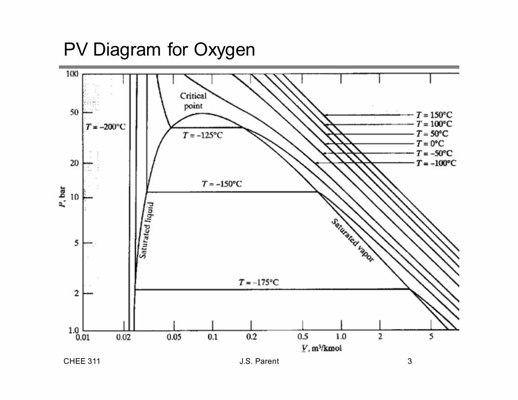
P-V-T Behaviour of a Pure Substance
The pure component PV-
diagram shown here
describes the
relationship between
pressure and molar
volume for the various
phases assumed by the
the substance.
CHEE 311 J.S. Parent 3
PV Diagram for Oxygen
CHEE 311 J.S. Parent 4
Equations of State
Experimental data exists for a great many substances and mixtures
over a wide range of conditions.
� Tabulated P-V-T data is cumbersome to catalogue and use
� Mathematical equations (Equations of State) describing
P-V-T behaviour are more commonly used to represent
segments of the phase diagram, usually gas-phase
behaviour
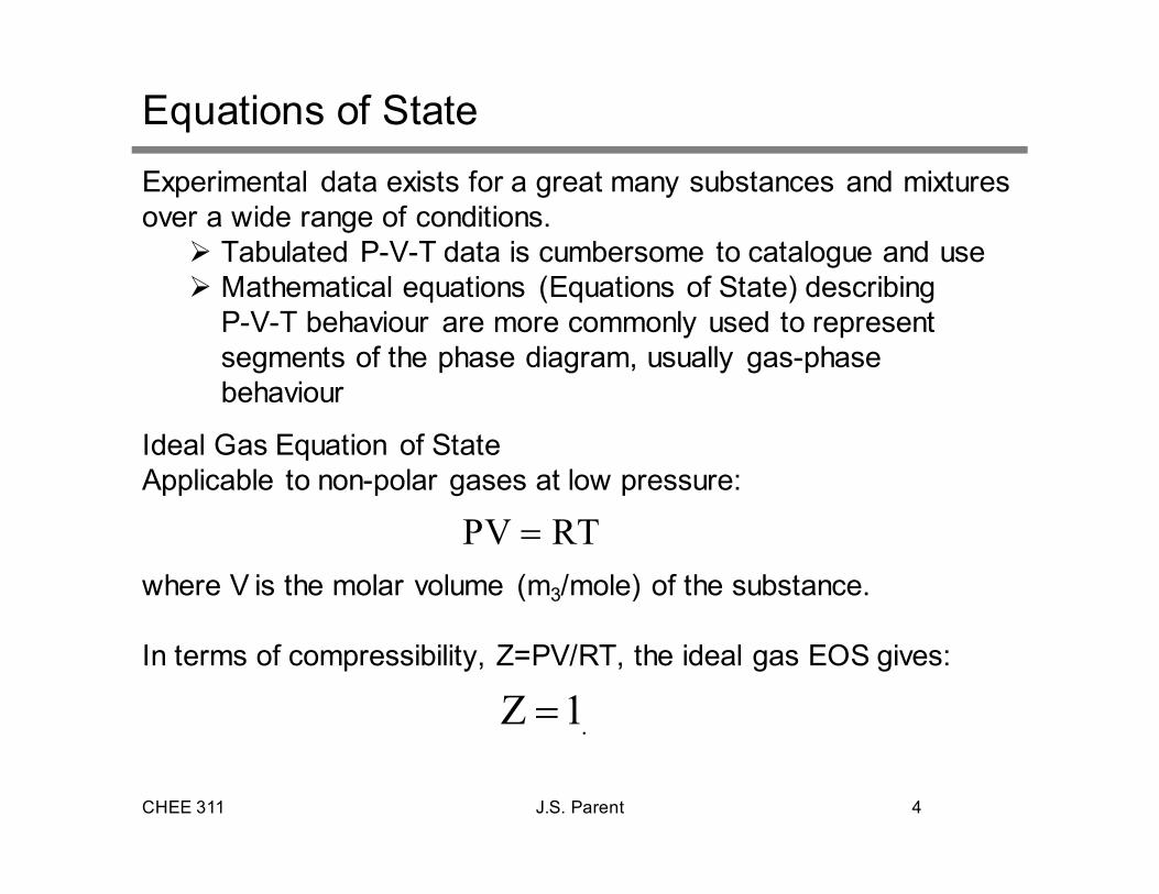
Ideal Gas Equation of State
Applicable to non-polar gases at low pressure:
where V is the molar volume (m3/mole) of the substance.
In terms of compressibility, Z=PV/RT, the ideal gas EOS gives:
PV RT=
.Z 1=
CHEE 311 J.S. Parent 5
Equations of State: Non-ideal Fluids
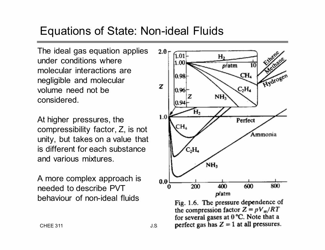
The ideal gas equation applies
under conditions where
molecular interactions are
negligible and molecular
volume need not be
considered.
At higher pressures, the
compressibility factor, Z, is not
unity, but takes on a value that
is different for each substance
and various mixtures.
A more complex approach is
needed to describe PVT
behaviour of non-ideal fluids
CHEE 311 J.S. Parent 6
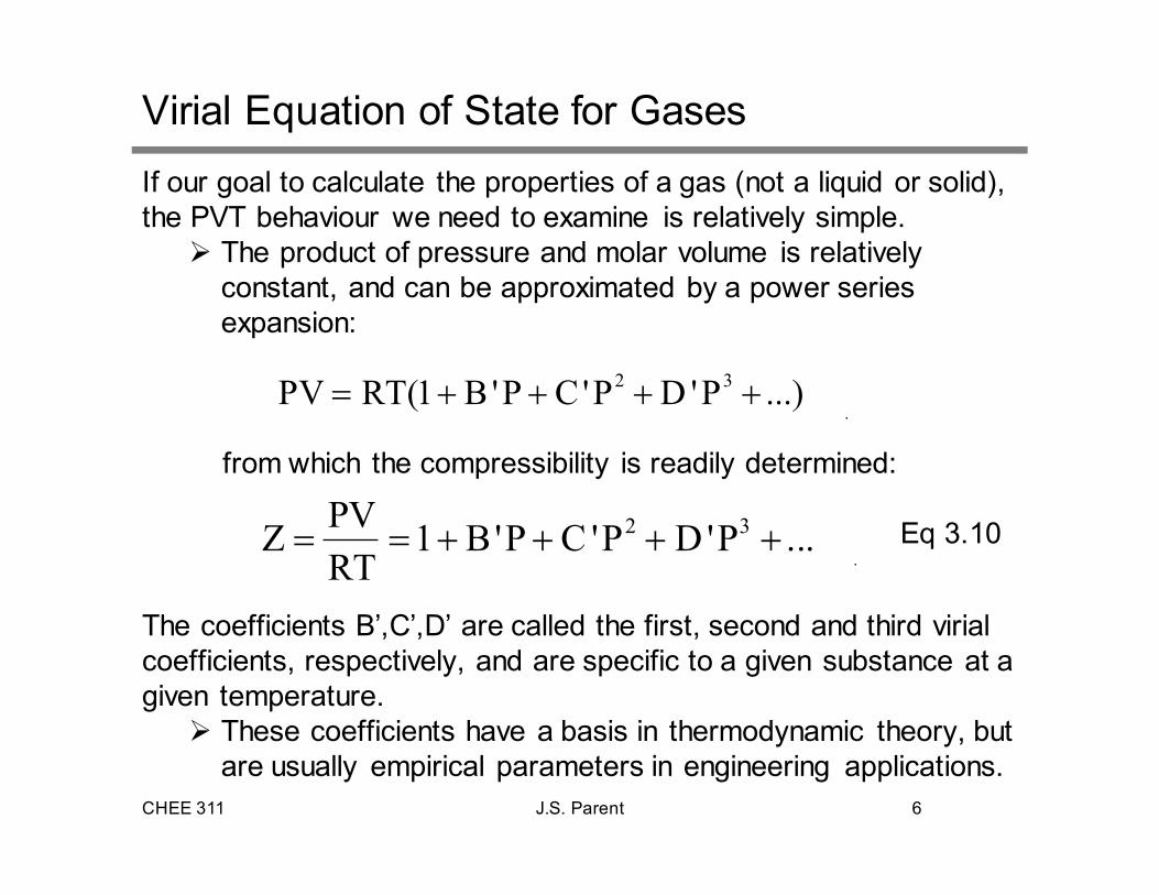
Virial Equation of State for Gases
If our goal to calculate the properties of a gas (not a liquid or solid),
the PVT behaviour we need to examine is relatively simple.
� The product of pressure and molar volume is relatively
constant, and can be approximated by a power series
expansion:
from which the compressibility is readily determined:
Eq 3.10
The coefficients B’,C’,D’ are called the first, second and third virial
coefficients, respectively, and are specific to a given substance at a
given temperature.
� These coefficients have a basis in thermodynamic theory, but
are usually empirical parameters in engineering applications.
.
2 3PV RT(1 B 'P C 'P D 'P ...)= + + + +
.
2 3PVZ 1 B'P C 'P D 'P ...
RT= = + + + +
CHEE 311 J.S. Parent 7
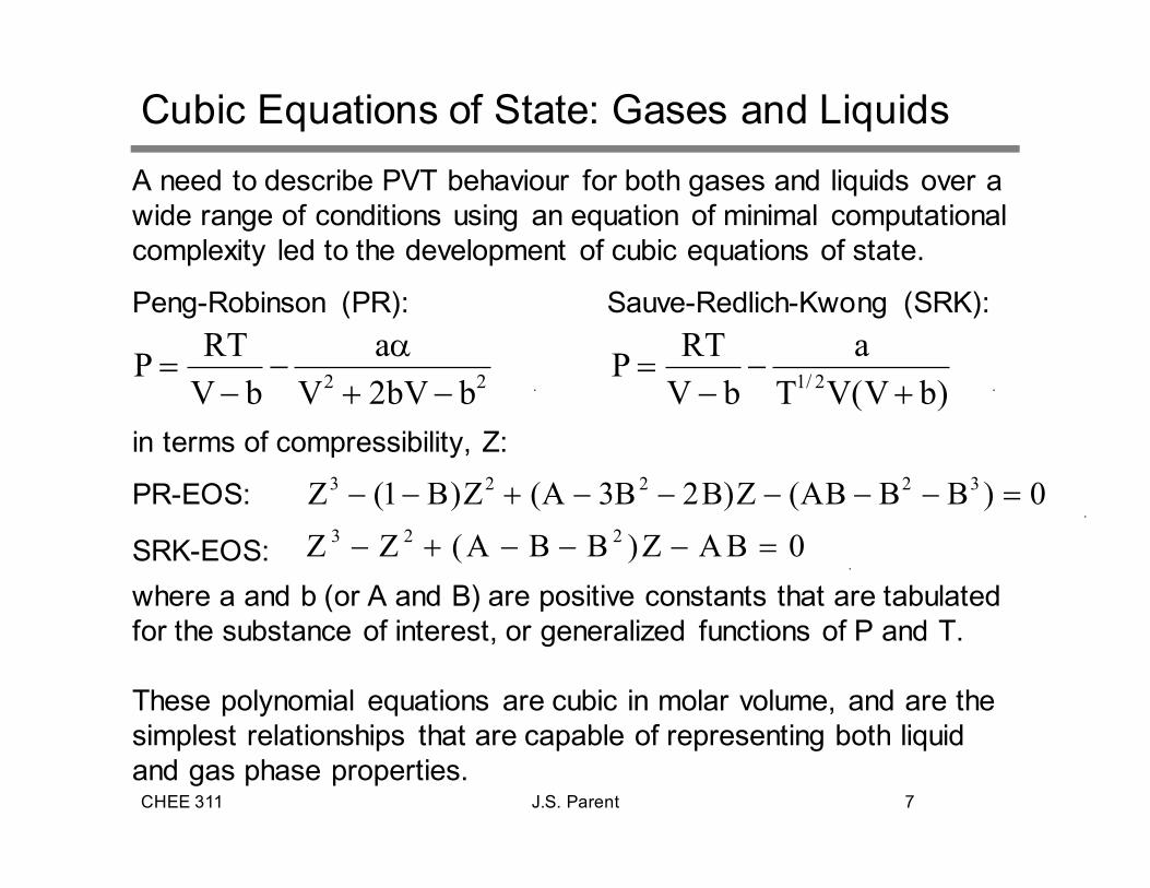
Cubic Equations of State: Gases and Liquids
A need to describe PVT behaviour for both gases and liquids over a
wide range of conditions using an equation of minimal computational
complexity led to the development of cubic equations of state.
Peng-Robinson (PR): Sauve-Redlich-Kwong (SRK):
in terms of compressibility, Z:
PR-EOS:
SRK-EOS:
where a and b (or A and B) are positive constants that are tabulated
for the substance of interest, or generalized functions of P and T.
These polynomial equations are cubic in molar volume, and are the
simplest relationships that are capable of representing both liquid
and gas phase properties.
.2 2
RT aP
V b V 2bV b
α= −
− + − .1/ 2
RT aP
V b T V(V b)= −
− +
.
3 2 2Z Z (A B B )Z AB 0− + − − − =.
3 2 2 2 3Z (1 B)Z (A 3B 2B)Z (AB B B ) 0− − + − − − − − =
CHEE 311 J.S. Parent 8
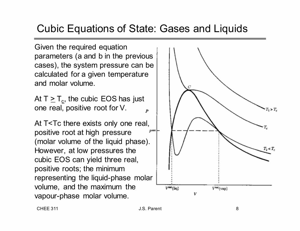
Cubic Equations of State: Gases and Liquids
Given the required equation
parameters (a and b in the previous
cases), the system pressure can be
calculated for a given temperature
and molar volume.
At T > Tc, the cubic EOS has just
one real, positive root for V.
At T<Tc there exists only one real,
positive root at high pressure
(molar volume of the liquid phase).
However, at low pressures the
cubic EOS can yield three real,
positive roots; the minimum
representing the liquid-phase molar
volume, and the maximum the
vapour-phase molar volume.
CHEE 311 J.S. Parent 9
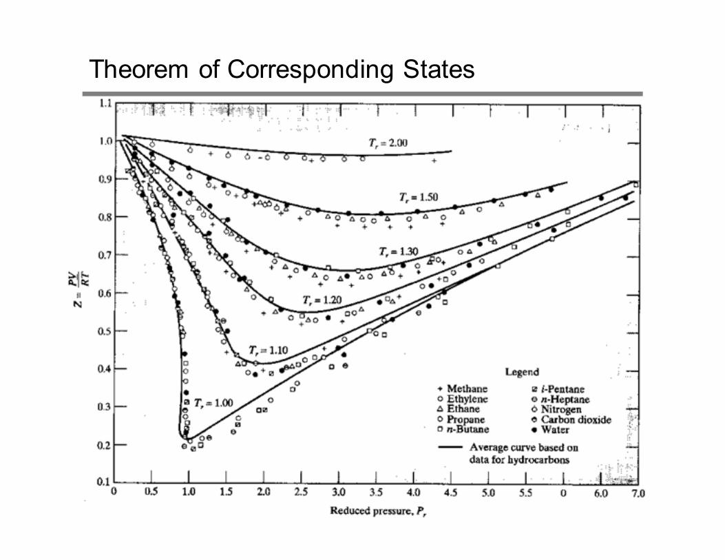
Theorem of Corresponding States
The virial and cubic equations of state require parameters (B’, C’, a,
b, for example) that are specific to the substance of interest. In
fact, the PVT relationships for most non-polar fluids is remarkably
similar when compared on the basis of reduced pressure and
temperature.
Simple fluids aside (argon, xenon, etc), some empiricism is
required to achieve the required degree of accuracy. The three-
parameter theorem of corresponding states is:
� All fluids having the same value of acentric factor, ω, when compared at the same Tr and Pr, have the same value of Z.
The advantage of the corresponding states, or generalized,
approach is that fluid properties can be estimated using very little
knowledge (Tc, Pc and ω) of the substance(s).
r
c
PP
P= r
c
TT
T=
CHEE 311 J.S. Parent 10
Theorem of Corresponding States
CHEE 311 J.S. Parent 11
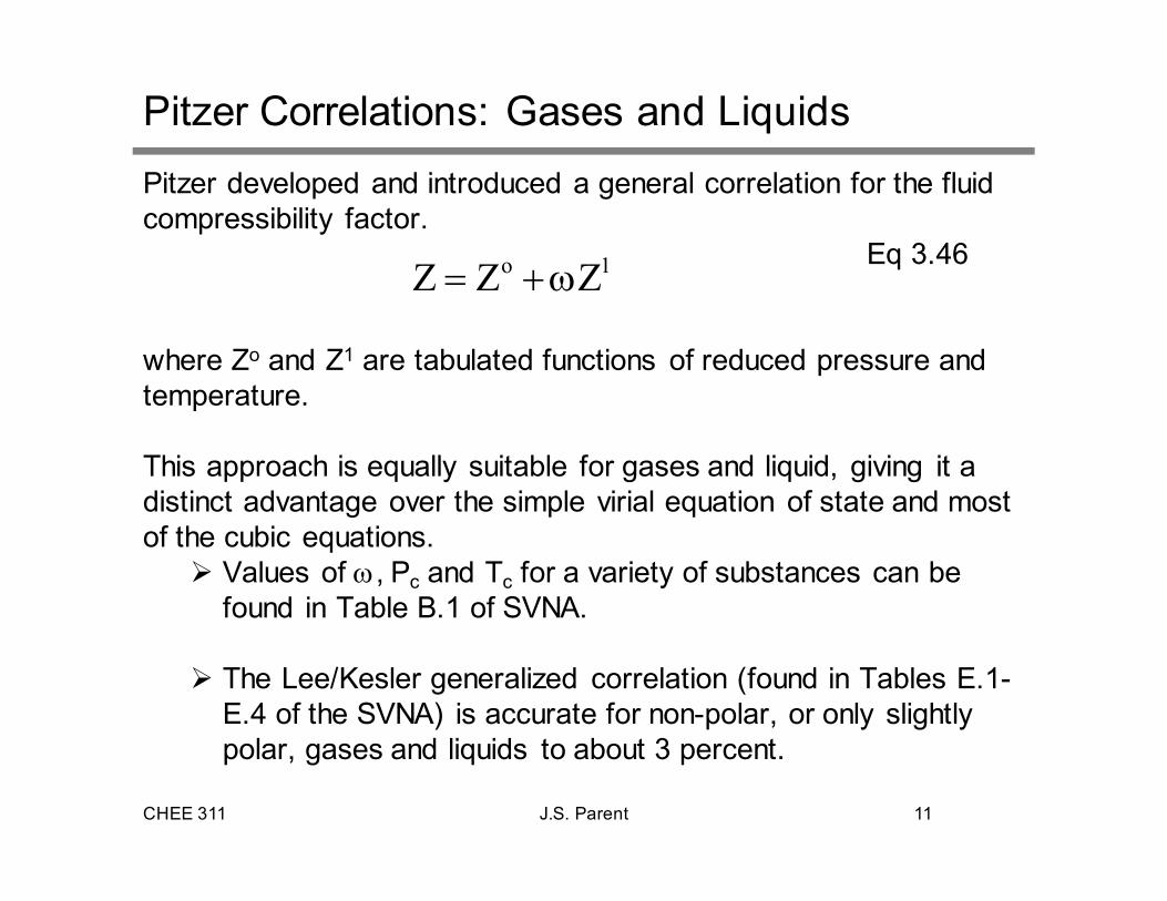
Pitzer Correlations: Gases and Liquids
Pitzer developed and introduced a general correlation for the fluid
compressibility factor.
Eq 3.46
where Zo and Z1 are tabulated functions of reduced pressure and
temperature.
This approach is equally suitable for gases and liquid, giving it a
distinct advantage over the simple virial equation of state and most
of the cubic equations.
� Values of ω, Pc and Tc for a variety of substances can be found in Table B.1 of SVNA.
� The Lee/Kesler generalized correlation (found in Tables E.1-
E.4 of the SVNA) is accurate for non-polar, or only slightly
polar, gases and liquids to about 3 percent.
o 1Z Z Z= +ω
CHEE 311 J.S. Parent 12
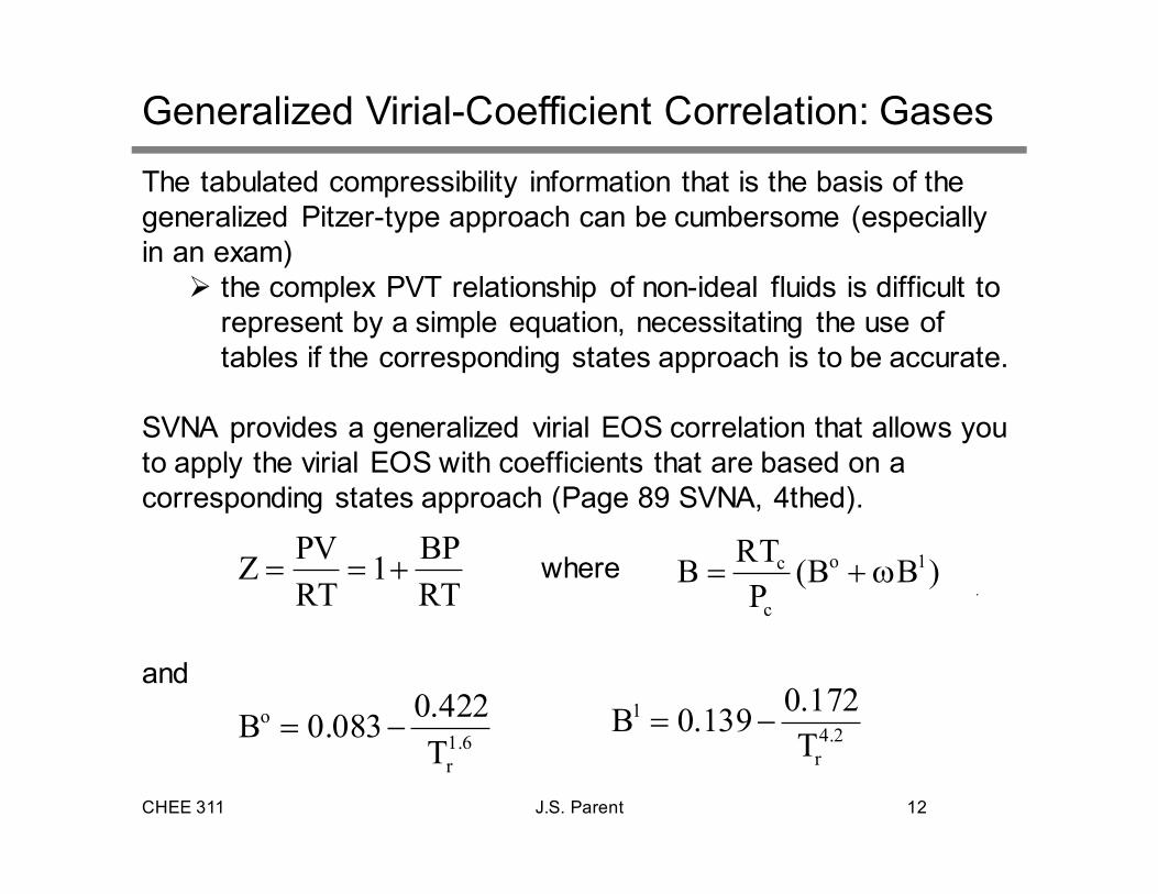
Generalized Virial-Coefficient Correlation: Gases
The tabulated compressibility information that is the basis of the
generalized Pitzer-type approach can be cumbersome (especially
in an exam)
� the complex PVT relationship of non-ideal fluids is difficult to
represent by a simple equation, necessitating the use of
tables if the corresponding states approach is to be accurate.
SVNA provides a generalized virial EOS correlation that allows you
to apply the virial EOS with coefficients that are based on a
corresponding states approach (Page 89 SVNA, 4thed).
where
and
PV BPZ 1
RT RT= = +
.
o 1c
c
RTB (B B )
P= + ω
o
1.6
r
0.422B 0.083
T= −
1
4.2
r
0.172B 0.139
T= −
CHEE 311 J.S. Parent 13
PVT Behaviour of Mixtures
Most equations of state prescribe mixing rules that allow you to
calculate EOS parameters and describe the PVT behaviour of
mixtures.
The Virial EOS,
the composition dependence of the virial coefficient B is:
where y represents the mole fractions in the mixture and the
indices i and j identify the species. Values of Bij are determined
using generalized correlations and/or formulae specifically
developed for the mixture of interest.
� Mixture behaviour will be examined in greater detail later in
the course
PVZ 1 BP
RT= = +
i j ij
i j
B y y B=∑∑
CHEE 311 J.S. Parent 14
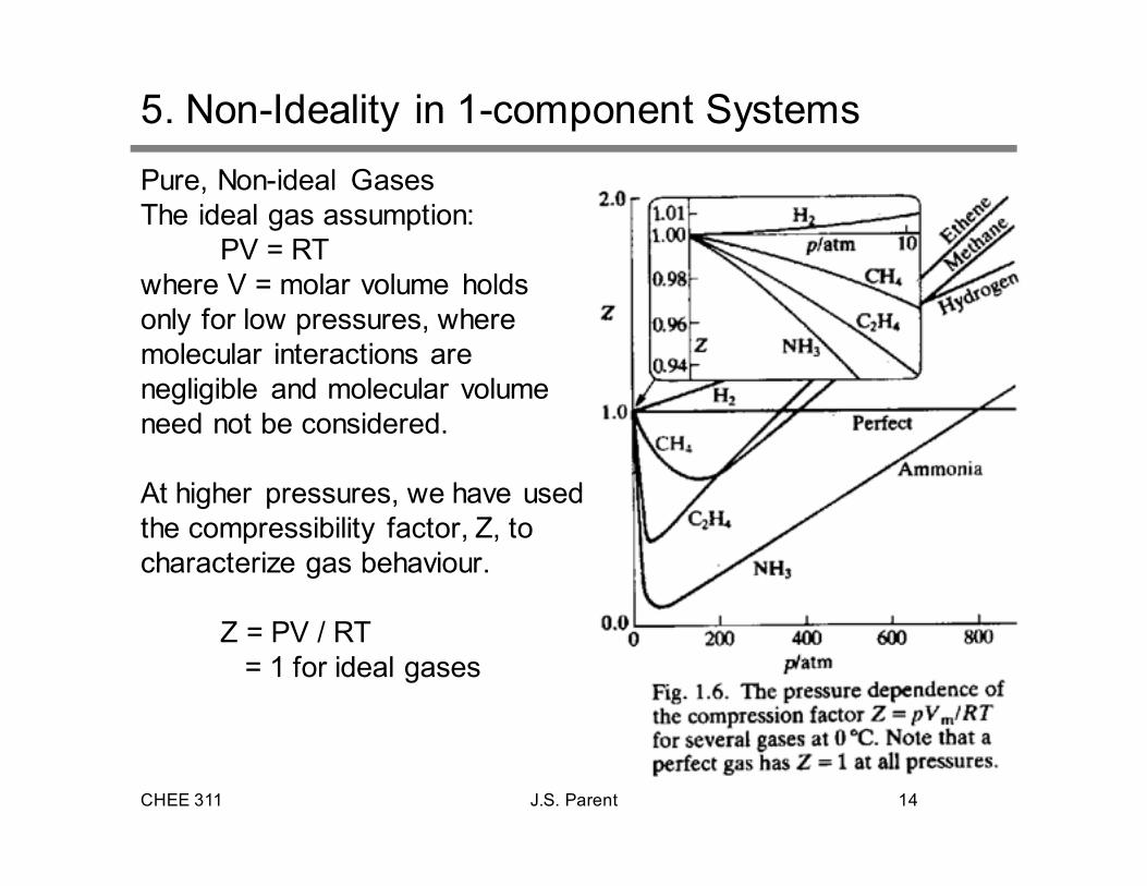
5. Non-Ideality in 1-component Systems
Pure, Non-ideal Gases
The ideal gas assumption:
PV = RT
where V = molar volume holds
only for low pressures, where
molecular interactions are
negligible and molecular volume
need not be considered.
At higher pressures, we have used
the compressibility factor, Z, to
characterize gas behaviour.
Z = PV / RT
= 1 for ideal gases
CHEE 311 J.S. Parent 15
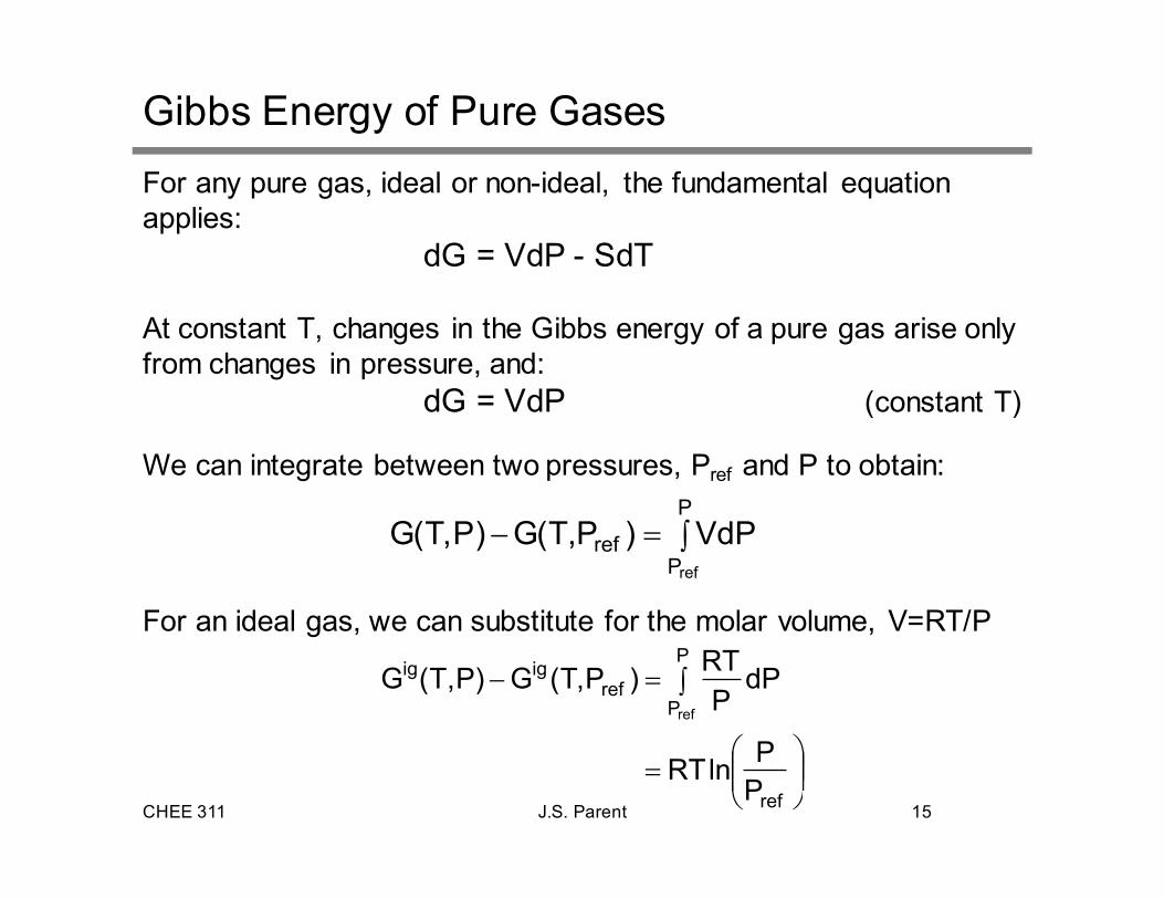
Gibbs Energy of Pure Gases
For any pure gas, ideal or non-ideal, the fundamental equation
applies:
dG = VdP - SdT
At constant T, changes in the Gibbs energy of a pure gas arise only
from changes in pressure, and:
dG = VdP (constant T)
We can integrate between two pressures, Pref and P to obtain:
For an ideal gas, we can substitute for the molar volume, V=RT/P
∫=−P
Pref
ref
VdP)P,T(G)P,T(G
=
∫=−
ref
P
Pref
igig
P
PlnRT
dPP
RT)P,T(G)P,T(G
ref
CHEE 311 J.S. Parent 16
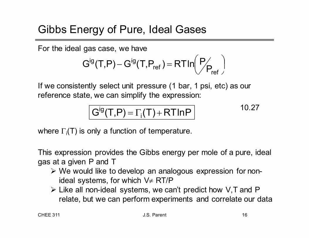
Gibbs Energy of Pure, Ideal Gases
For the ideal gas case, we have
If we consistently select unit pressure (1 bar, 1 psi, etc) as our
reference state, we can simplify the expression:
10.27
where Γi(T) is only a function of temperature.
This expression provides the Gibbs energy per mole of a pure, ideal
gas at a given P and T
� We would like to develop an analogous expression for non-
ideal systems, for which V≠ RT/P� Like all non-ideal systems, we can’t predict how V,T and P
relate, but we can perform experiments and correlate our data
=−
refref
igig
PPlnRT)P,T(G)P,T(G
PlnRT)T()P,T(G iig +Γ=
CHEE 311 J.S. Parent 17
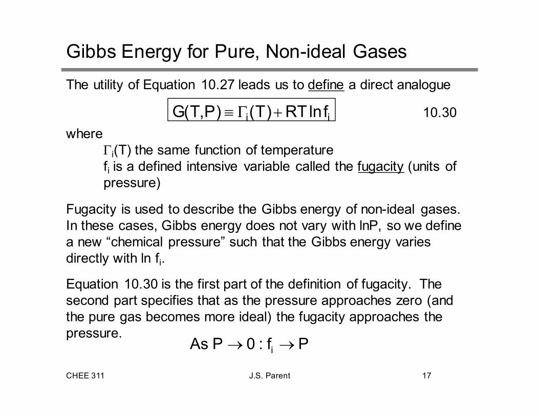
Gibbs Energy for Pure, Non-ideal Gases
The utility of Equation 10.27 leads us to define a direct analogue
10.30
where
Γi(T) the same function of temperaturefi is a defined intensive variable called the fugacity (units of
pressure)
Fugacity is used to describe the Gibbs energy of non-ideal gases.
In these cases, Gibbs energy does not vary with lnP, so we define
a new “chemical pressure” such that the Gibbs energy varies
directly with ln fi.
Equation 10.30 is the first part of the definition of fugacity. The
second part specifies that as the pressure approaches zero (and
the pure gas becomes more ideal) the fugacity approaches the
pressure.
ii flnRT)T()P,T(G +Γ≡
Pf:0PAs i →→
CHEE 311 J.S. Parent 18
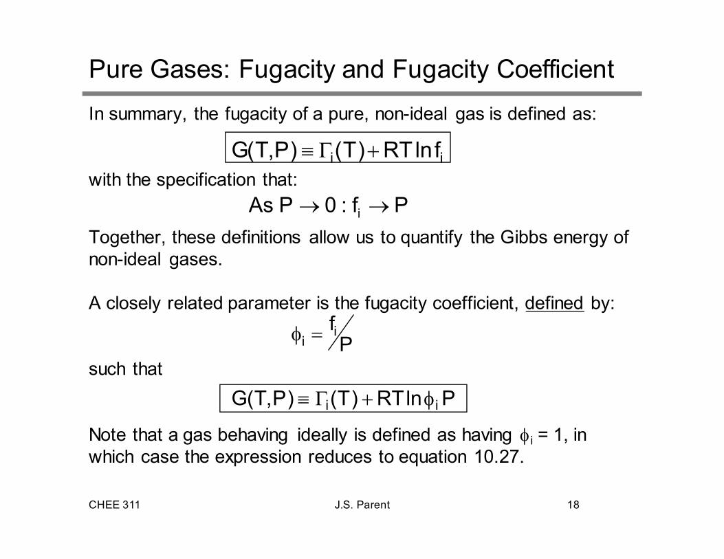
Pure Gases: Fugacity and Fugacity Coefficient
In summary, the fugacity of a pure, non-ideal gas is defined as:
with the specification that:
Together, these definitions allow us to quantify the Gibbs energy of
non-ideal gases.
A closely related parameter is the fugacity coefficient, defined by:
such that
Note that a gas behaving ideally is defined as having φi = 1, in which case the expression reduces to equation 10.27.
Pfi
i =φ
PlnRT)T()P,T(G ii φ+Γ≡
ii flnRT)T()P,T(G +Γ≡
Pf:0PAs i →→
CHEE 311 J.S. Parent 19
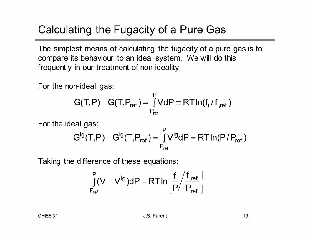
Calculating the Fugacity of a Pure Gas
The simplest means of calculating the fugacity of a pure gas is to
compare its behaviour to an ideal system. We will do this
frequently in our treatment of non-ideality.
For the non-ideal gas:
For the ideal gas:
Taking the difference of these equations:
=∫ −
ref
ref,iiP
P
ig
P
f
P
flnRTdP)VV(
ref
)f/fln(RTVdP)P,T(G)P,T(G ref,ii
P
Pref
ref
≡∫=−
)P/Pln(RTdPV)P,T(G)P,T(G ref
P
P
igref
igig
ref
=∫=−
CHEE 311 J.S. Parent 20
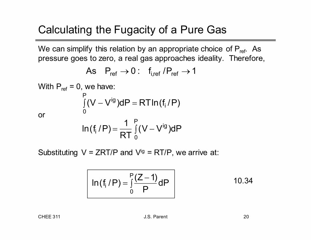
Calculating the Fugacity of a Pure Gas
We can simplify this relation by an appropriate choice of Pref. As
pressure goes to zero, a real gas approaches ideality. Therefore,
With Pref = 0, we have:
or
Substituting V = ZRT/P and Vig = RT/P, we arrive at:
10.34
1P/f:0PAs refref,iref →→
)P/f(lnRTdP)VV( i
P
0
ig =∫ −
∫ −=P
0
igi dP)VV(
RT
1)P/f(ln
∫−
=P
0i dP
P
)1Z()P/f(ln
CHEE 311 J.S. Parent 21
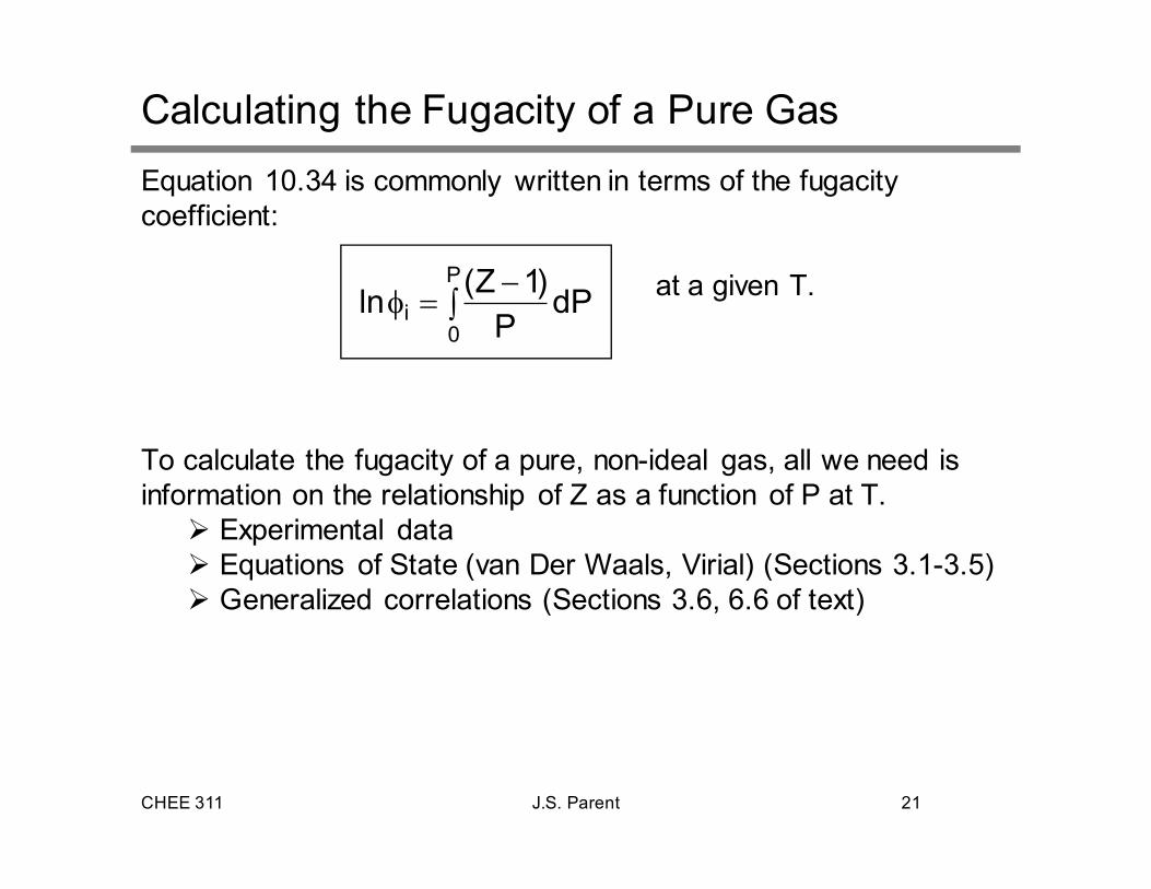
Calculating the Fugacity of a Pure Gas
Equation 10.34 is commonly written in terms of the fugacity
coefficient:
at a given T.
To calculate the fugacity of a pure, non-ideal gas, all we need is
information on the relationship of Z as a function of P at T.
� Experimental data
� Equations of State (van Der Waals, Virial) (Sections 3.1-3.5)
� Generalized correlations (Sections 3.6, 6.6 of text)
∫−
=φP
0i dP
P
)1Z(ln
CHEE 311 J.S. Parent 22
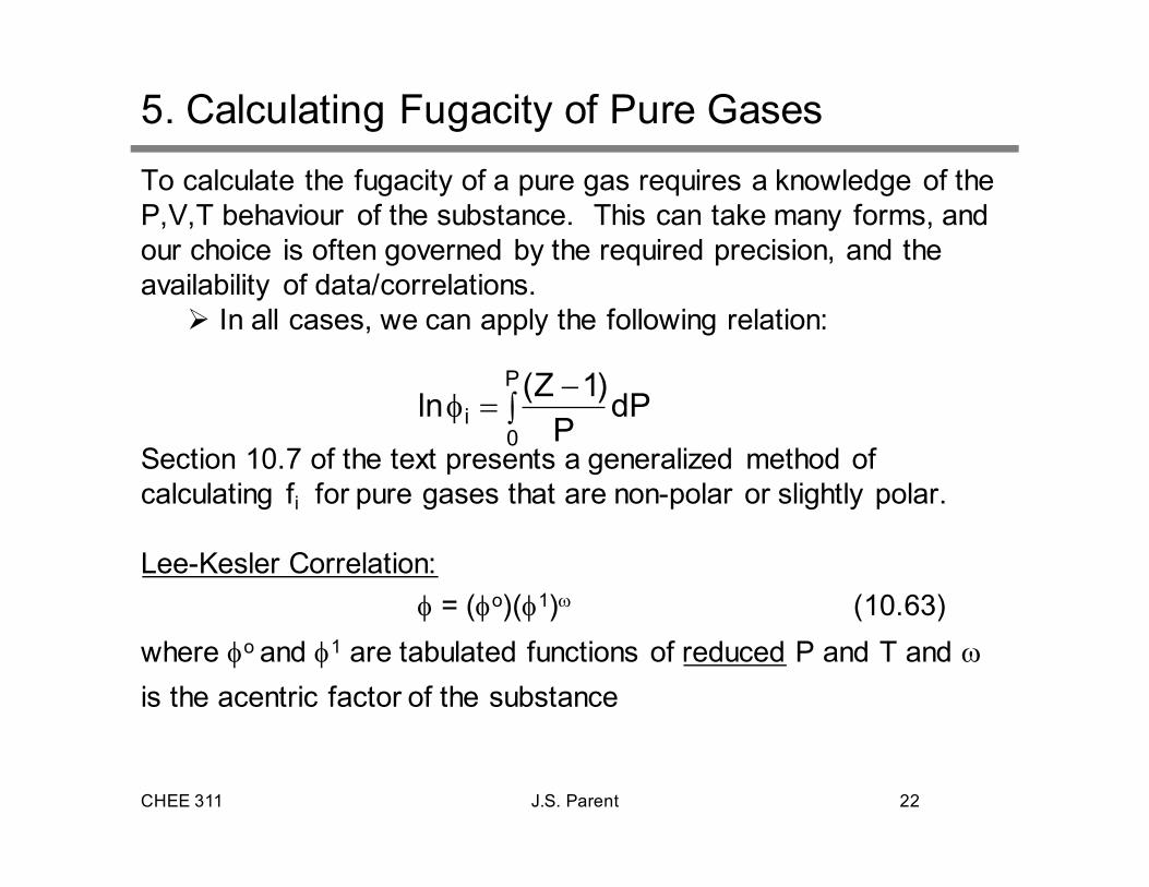
5. Calculating Fugacity of Pure Gases
To calculate the fugacity of a pure gas requires a knowledge of the
P,V,T behaviour of the substance. This can take many forms, and
our choice is often governed by the required precision, and the
availability of data/correlations.
� In all cases, we can apply the following relation:
Section 10.7 of the text presents a generalized method of
calculating fi for pure gases that are non-polar or slightly polar.
Lee-Kesler Correlation:
φ = (φo)(φ1)ω (10.63)
where φo and φ1 are tabulated functions of reduced P and T and ω
is the acentric factor of the substance
∫−
=φP
0i dP
P
)1Z(ln
CHEE 311 J.S. Parent 23
Calculating Fugacity of Pure Gases
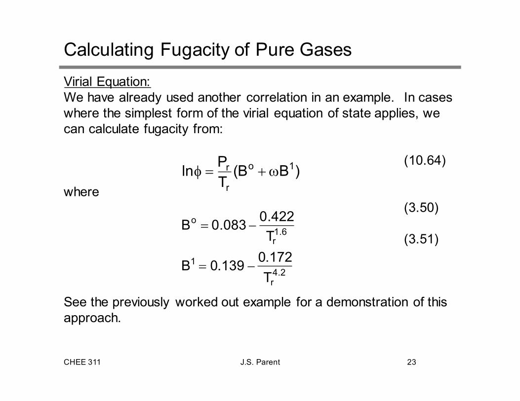
Virial Equation:
We have already used another correlation in an example. In cases
where the simplest form of the virial equation of state applies, we
can calculate fugacity from:
(10.64)
where
(3.50)
(3.51)
See the previously worked out example for a demonstration of this
approach.
)BB(T
Pln 1o
r
r ω+=φ
2.4r
1
6.1r
o
T
172.0139.0B
T
422.0083.0B
−=
−=
CHEE 311 J.S. Parent 24
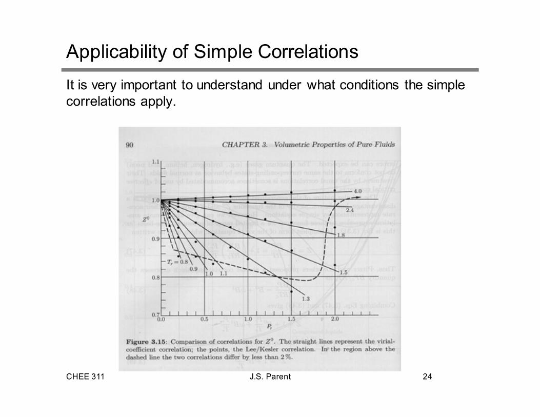
Applicability of Simple Correlations
It is very important to understand under what conditions the simple
correlations apply.
CHEE 311 J.S. Parent 25
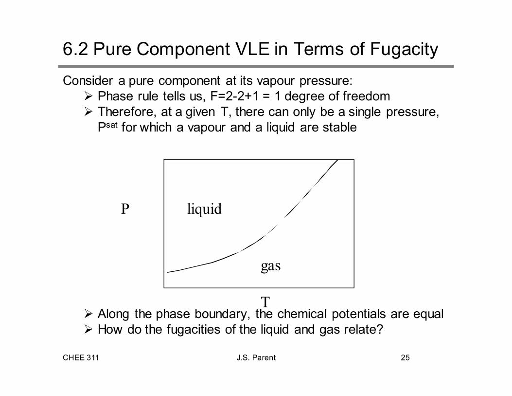
6.2 Pure Component VLE in Terms of Fugacity
Consider a pure component at its vapour pressure:
� Phase rule tells us, F=2-2+1 = 1 degree of freedom
� Therefore, at a given T, there can only be a single pressure,
Psat for which a vapour and a liquid are stable
� Along the phase boundary, the chemical potentials are equal
� How do the fugacities of the liquid and gas relate?
P liquid
gas
T
CHEE 311 J.S. Parent 26
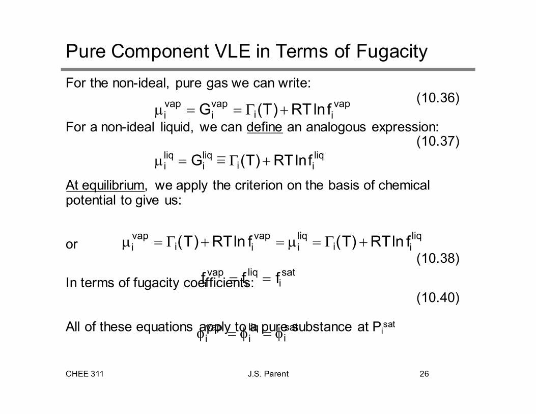
Pure Component VLE in Terms of Fugacity
For the non-ideal, pure gas we can write:(10.36)
For a non-ideal liquid, we can define an analogous expression:(10.37)
At equilibrium, we apply the criterion on the basis of chemical potential to give us:
or(10.38)
In terms of fugacity coefficients:(10.40)
All of these equations apply to a pure substance at Pisat
liqii
liqi
vapii
vapi flnRT)T(flnRT)T( +Γ=µ=+Γ=µ
vapii
vapi
vapi flnRT)T(G +Γ==µ
sati
liqi
vapi fff ==
sati
liqi
vapi φ=φ=φ
liqii
liqi
liqi flnRT)T(G +Γ==µ
CHEE 311 J.S. Parent 27
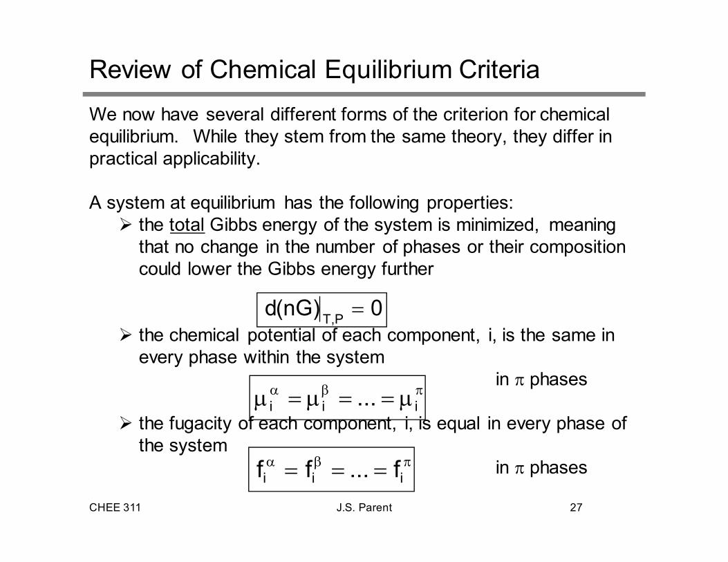
Review of Chemical Equilibrium Criteria
We now have several different forms of the criterion for chemical
equilibrium. While they stem from the same theory, they differ in
practical applicability.
A system at equilibrium has the following properties:
� the total Gibbs energy of the system is minimized, meaning
that no change in the number of phases or their composition
could lower the Gibbs energy further
� the chemical potential of each component, i, is the same in
every phase within the system
in π phases
� the fugacity of each component, i, is equal in every phase of
the system
in π phasesπβα === iii f...ff
πβα µ==µ=µ iii ...
0)nG(dP,T=
CHEE 311 J.S. Parent 28
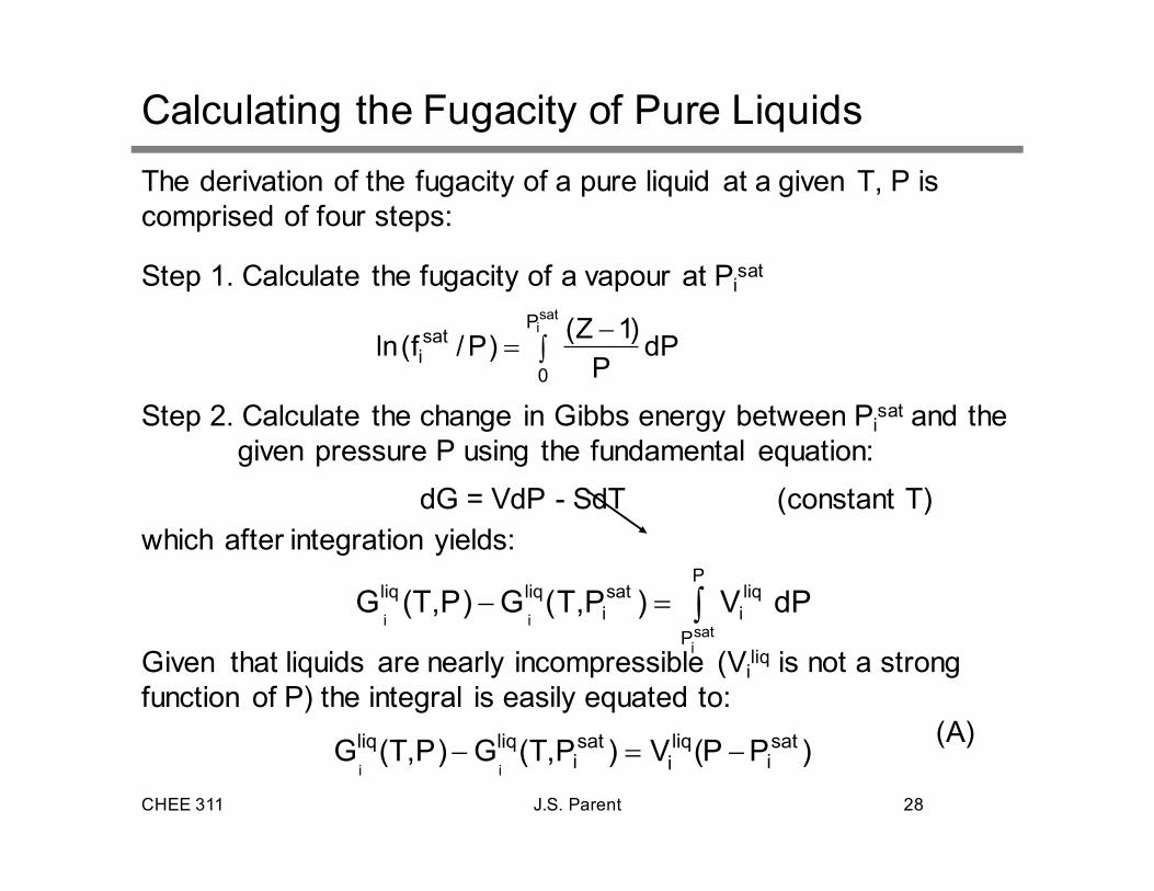
Calculating the Fugacity of Pure Liquids
The derivation of the fugacity of a pure liquid at a given T, P is
comprised of four steps:
Step 1. Calculate the fugacity of a vapour at Pisat
Step 2. Calculate the change in Gibbs energy between Pisat and the
given pressure P using the fundamental equation:
dG = VdP - SdT (constant T)
which after integration yields:
Given that liquids are nearly incompressible (Viliq is not a strong
function of P) the integral is easily equated to:
(A)
∫−
=satiP
0
sati dP
P
)1Z()P/f(ln
dPV)P,T(G)P,T(GP
P
liq
i
sat
i
liqliq
sati
ii ∫=−
)PP(V)P,T(G)P,T(G sati
liqi
sati
liqliq
ii−=−
CHEE 311 J.S. Parent 29
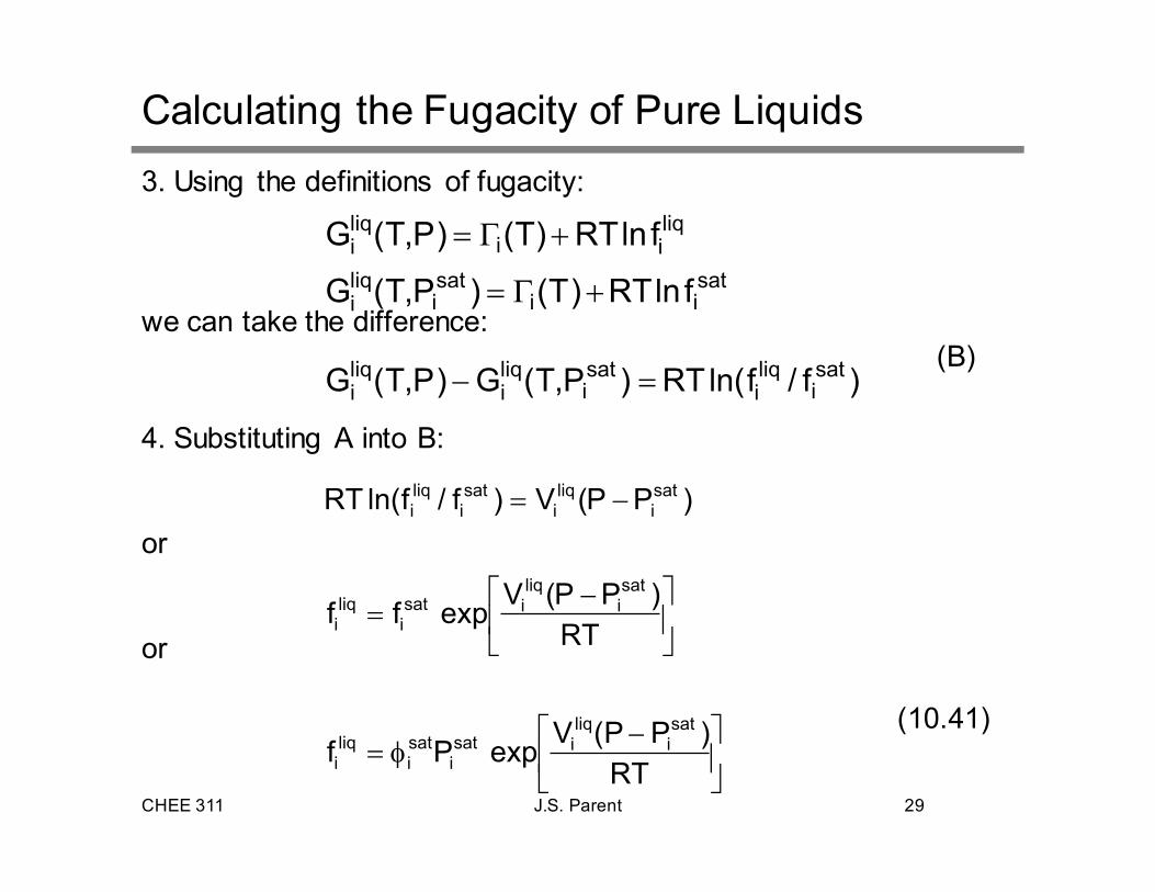
Calculating the Fugacity of Pure Liquids
3. Using the definitions of fugacity:
we can take the difference:
(B)
4. Substituting A into B:
or
or
(10.41)
satii
sati
liqi
liqii
liqi
flnRT)T()P,T(G
flnRT)T()P,T(G
+Γ=
+Γ=
)f/fln(RT)P,T(G)P,T(G sati
liqi
sati
liqi
liqi =−
−φ=
−=
−=
RT
)PP(VexpPf
RT
)PP(Vexpff
)PP(V)f/fln(RT
sati
liqisat
isati
liqi
sati
liqisat
iliqi
sati
liqi
sati
liqi
CHEE 311 J.S. Parent 30
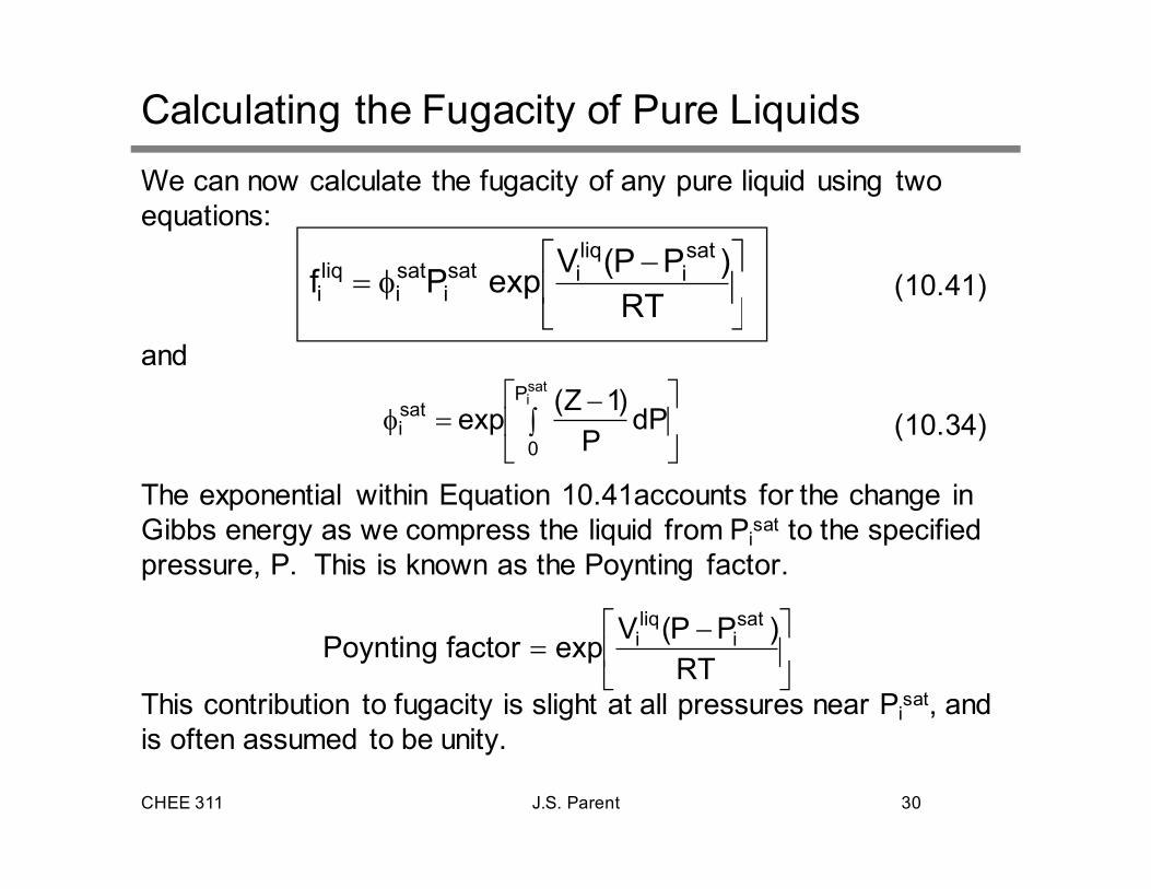
Calculating the Fugacity of Pure Liquids
We can now calculate the fugacity of any pure liquid using two
equations:
(10.41)
and
(10.34)
The exponential within Equation 10.41accounts for the change in
Gibbs energy as we compress the liquid from Pisat to the specified
pressure, P. This is known as the Poynting factor.
This contribution to fugacity is slight at all pressures near Pisat, and
is often assumed to be unity.
−φ=
RT
)PP(VexpPf
sati
liqisat
isati
liqi
∫
−=φ
satiP
0
sati dP
P
)1Z(exp
−=
RT
)PP(VexpfactorPoynting
sati
liqi