1

5. Atomic radiation processes

Einstein coefficients for absorption and emission

oscillator strength

line profiles: damping profile, collisional

broadening, Doppler broadening

continuous absorption and scattering

2

3

A. Line transitionsA. Line transitions

Einstein coefficients

probability that a photon in frequency interval in the solid angle range is absorbed by an atom in the energy level El

with a resulting transition El

Eu

per second:

atomic property ~ no. of incident photons

probability for absorption of photon with

absorption profile

probability for with

probability for transition l u

Blu : Einstein coefficient for absorption

dwabs(ν, ω, l,u) =Blu Iν(ω) ϕ(ν)dν dω4π

4

Einstein coefficients

similarly for stimulated emission

Bul : Einstein coefficient for stimulated emission

and for spontaneous emission

Aul : Einstein coefficient for spontaneous emission

dwst(ν,ω, l ,u) = Bul Iν(ω) ϕ(ν)dν dω4π

dwsp(ν, ω, l,u) =Aul ϕ(ν)dν dω4π

5

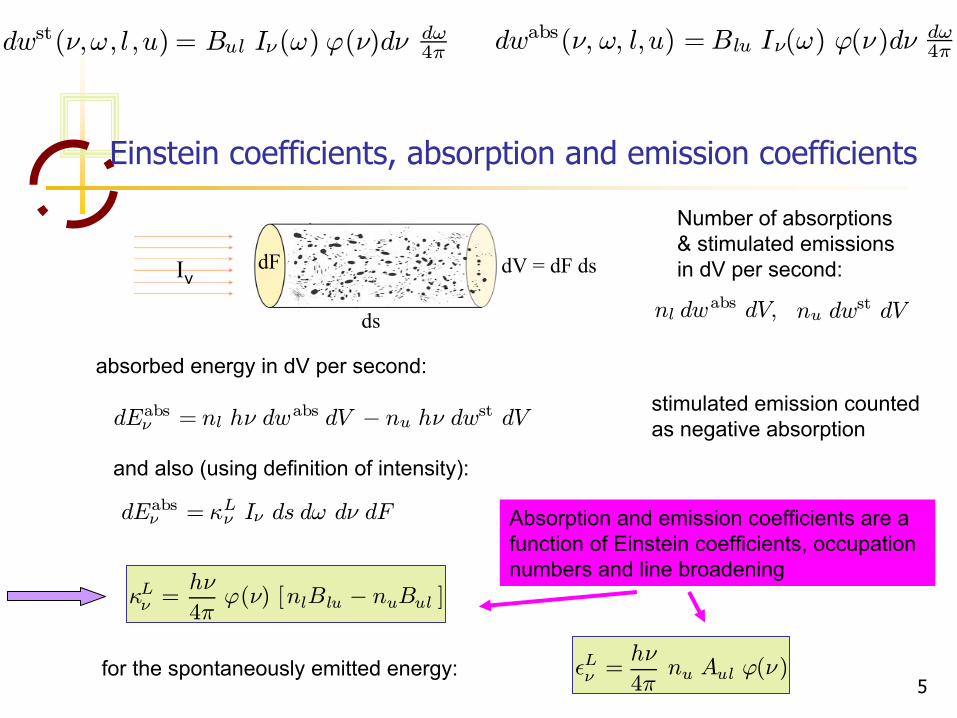
Einstein coefficients, absorption and emission coefficients

Iν dF

ds

dV

= dF

ds

absorbed energy in dV

per second:

dEabsν = nl hν dwabs dV − nu hν dwst dV

and also (using definition of intensity):

for the spontaneously emitted energy:

κLν =hν

4πϕ(ν) [nlBlu − nuBul ]

²Lν =hν

4πnu Aul ϕ(ν)

dwst(ν,ω, l ,u) = Bul Iν(ω) ϕ(ν)dν dω4π dwabs(ν, ω, l,u) =Blu Iν(ω) ϕ(ν)dν dω

4π

dEabsν = κLν Iν ds dω dν dF

Number of absorptions & stimulated emissions in dV

per second:

nu dwst dVnl dw

abs dV,

stimulated emission counted as negative absorption

Absorption and emission coefficients are a function of Einstein coefficients, occupation numbers and line broadening

6

Einstein coefficients are atomic properties do not depend on thermodynamic state of matter

We can assume TE: Sν =²LνκLν

= Bν(T)

Bν(T) =nuAul

nlBlu− nuBul=nunl

AulBlu− nu

nlBul

From the Boltzmann formula:

for hν/kT

<< 1:nunl=gugl

µ1− hν

kT

¶, Bν(T) =

2ν2

c2kT

2ν2

c2kT =

gugl

µ1− hν

kT

¶Aul

Blu− gugl

¡1 − hν

kT

¢Bul

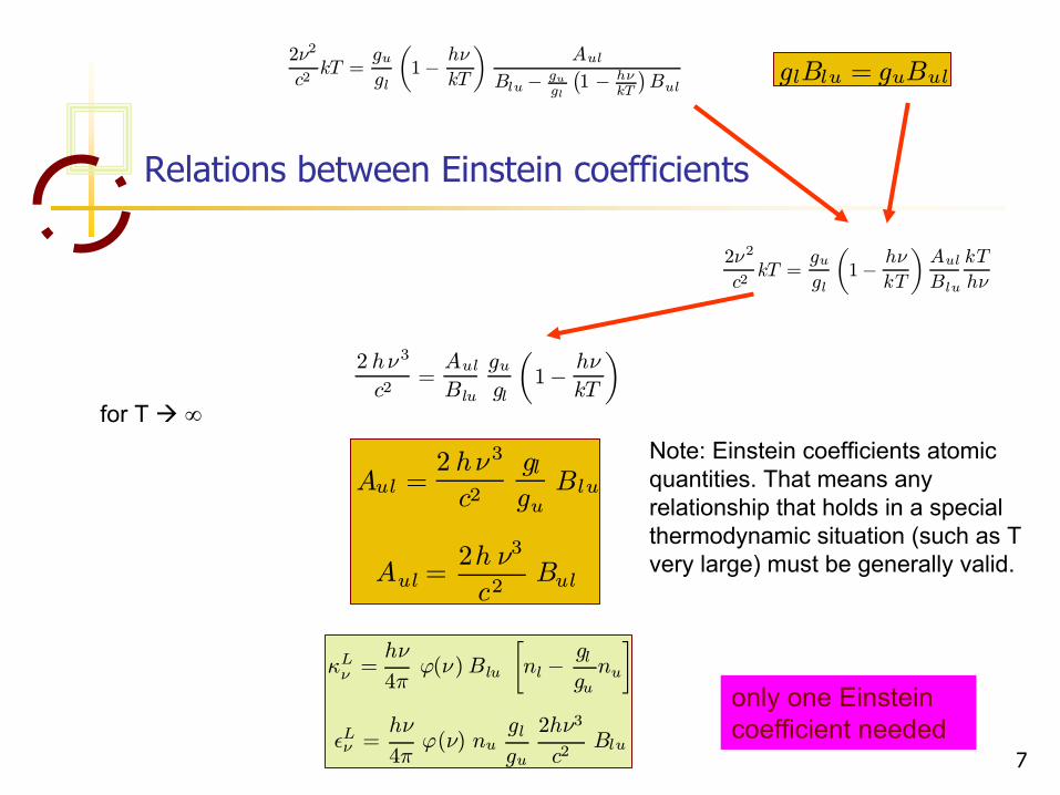
for T ∞ 0 glBlu = guBul

Relations between Einstein coefficients

nu

nl=gu

gle−

hνkT

κLν =hν

4πϕ(ν) [nlBlu − nuBul ] ²Lν =

hν

4πnu Aul ϕ(ν)

7

Relations between Einstein coefficients

2 hν3

c2=AulBlu

gugl

µ1− hν

kT

¶

Aul =2 hν3

c2glguBlu

Aul =2h ν3

c2Bul

κLν =hν

4πϕ(ν)Blu

·nl −

glgunu

¸

²Lν =hν

4πϕ(ν) nu

glgu

2hν3

c2Blu

only one Einstein coefficient needed

Note: Einstein coefficients atomic quantities. That means any relationship that holds in a special thermodynamic situation (such as T very large) must be generally valid.

glBlu = guBul2ν2

c2kT =

gugl

µ1− hν

kT

¶Aul

Blu− gugl

¡1 − hν

kT

¢Bul

2ν2

c2kT =

gugl

µ1− hν

kT

¶AulBlu

kT

hν

for T ∞

8

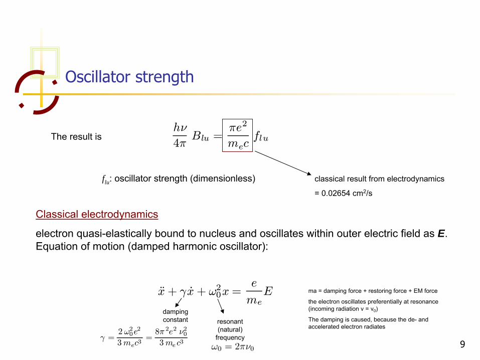
Oscillator strength

Quantum mechanics

The Einstein coefficients can be calculated by quantum mechanics + classical electrodynamics calculation.

Eigenvalue

problem using using

wave function:

Consider a time-dependent perturbation such as an external electromagnetic field (light wave) E(t) = E0

eiωt.

The potential of the time dependent perturbation on the atom is:

Hatom |ψl >= El |ψl > Hatom =p2

2m+ Vnucleus + Vshell

V (t) = eNXi=1

E · ri = E · d d: dipol

operator

[Hatom + V (t)] |ψl >= El |ψl >

with transition probability ∼ | < ψl|d|ψu > |2

9

Oscillator strength

flu : oscillator strength (dimensionless)

hν

4πBlu =

πe2

mecflu

classical result from electrodynamics

= 0.02654 cm2/s

The result is

Classical electrodynamics

electron quasi-elastically bound to nucleus and oscillates within outer electric field as E. Equation of motion (damped harmonic oscillator):

x+ γx+ ω20x=e

meE

damping constant resonant

(natural) frequency

ma = damping force + restoring force + EM force

the electron oscillates preferentially at resonance (incoming radiation ν

= ν0

)

The damping is caused, because the de-

and accelerated electron radiates

γ =2 ω20e

2

3mec3=8π 2e2 ν203mec3

10

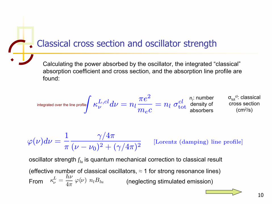
Classical cross section and oscillator strength

Calculating the power absorbed by the oscillator, the integrated

“classical”

absorption coefficient and cross section, and the absorption line profile are found:

nl : number density of absorbers

oscillator strength flu is quantum mechanical correction to classical result

(effective number of classical oscillators, ≈

1 for strong resonance lines)

From (neglecting

stimulated emission)

integrated over the line profile

κLν =hν

4πϕ(ν) nlBlu

σtotcl: classical

cross section (cm2/s)

ZκL,clν dν = nl

πe2

mec= nl σ

cltot

ϕ(ν)dν =1

π

γ/4π

(ν − ν0)2 + (γ/4π)2[Lorentz (damping) line profile]

11

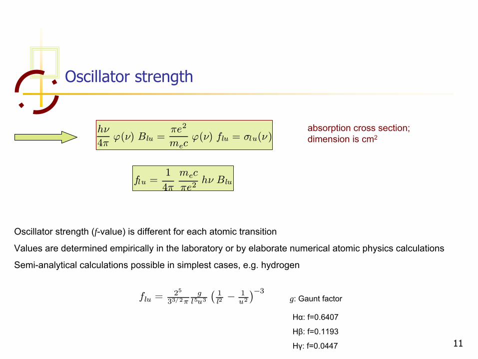
Oscillator strength

hν

4πϕ(ν) Blu =

πe2

mecϕ(ν) flu = σlu(ν)

absorption cross section; dimension is cm2

flu =1

4π

mec

πe2hν Blu

Oscillator strength (f-value) is different for each atomic transition

Values are determined empirically in the laboratory or by elaborate numerical atomic physics calculations

Semi-analytical calculations possible in simplest cases, e.g. hydrogen

flu =25

33/2πg

l5u3

¡1l2− 1

u2

¢−3g: Gaunt factor

Hα: f=0.6407

Hβ: f=0.1193

Hγ: f=0.0447

12

Line profilesLine profiles

line profiles contain information on physical conditions of the gas and chemical abundances

analysis of line profiles requires knowledge of distribution of opacity with frequency

several mechanisms lead to line broadening (no infinitely sharp lines)

-

natural damping: finite lifetime of atomic levels

-

collisional

(pressure) broadening: impact vs

quasi-static approximation

-

Doppler broadening: convolution of velocity distribution with atomic profiles

13

1. Natural damping profile

finite lifetime of atomic levels line width

NATURAL

LINE BROADENING

OR

RADIATION

DAMPING

line broadening

Lorentzian

profile

ϕ(ν) =1

π

Γ/4π

(ν − ν0)2 + (Γ/4π)2

t

= 1 / Aul

(¼

10-8

s in H atom 2 1):

finite lifetime with respect to spontaneous emission

Δ

E t

≥

h/2π

uncertainty principle

Δν1/2

= Γ

/ 2π

Δλ1/2

=

Δν1/2

λ2/c

e.g. Ly α: Δλ1/2

= 1.2 10-4

A

Hα: Δλ1/2

= 4.6 10-4

A

14

Natural damping profile

resonance line

natural line broadening is important for strong lines

(resonance lines) at low densities

(no additional broadening mechanisms)

e.g. Ly α

in interstellar medium

but also in stellar atmospheres

excited line

15

2. Collisional

broadening

a) impact approximation: radiating atoms are perturbed by passing particles at distance r(t). Duration of collision << lifetime in level lifetime shortened line broader

in all cases a Lorentzian profile is obtained (but with larger total Γ

than

only natural damping)

b) quasi-static approximation: applied when duration of collisions >> life time in level

consider stationary distribution of perturbers

r: distance to perturbing atom

radiating atoms are perturbed by the electromagnetic field of neighbour

atoms, ions, electrons, molecules

energy levels are temporarily modified through the Stark -

effect: perturbation is a function of separation absorber-perturber

energy levels affected line shifts, asymmetries & broadening

ΔE(t) = h Δν

= C/rn(t)

16

Collisional

broadening

n = 2

linear Stark effect ΔE ~ F

for levels with degenerate angular momentum (e.g. HI, HeII)

field strength F ~

1/r2

ΔE ~

1/r2

important for H I lines, in particular in hot stars (high number density of free electrons and ions). However , for ion collisional

broadening the quasi-static broadening is also important for strong lines (see below) Γe

~ ne

n = 3

resonance broadeningatom A perturbed by atom A’

of same species

important in cool stars, e.g. Balmer

lines in the Sun

ΔE ~

1/r3 Γe

~ ne

17

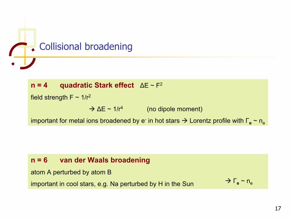
Collisional

broadening

n = 6

van der

Waals broadeningatom A perturbed by atom B

important in cool stars, e.g. Na perturbed by H in the Sun

n = 4

quadratic Stark effect ΔE ~

F2

field strength F ~

1/r2

ΔE ~

1/r4

(no dipole moment)

important for metal ions broadened by e-

in hot stars Lorentz profile with Γe

~ ne

Γe

~ ne

18

Quasi-static approximation

tperturbation

>>

τ

= 1/Aul

perturbation practically constant during emission or absorption

atom radiates in a statistically fluctuating field produced

by ‘quasi-static’

perturbers,

e.g. slow-moving ions

given a distribution of perturbers

field at location of absorbing or emitting atom

statistical frequency of particle distribution

probability of fields of different strength (each producing an energy shift ΔE = h Δν)

field strength distribution function

line broadening

Linear Stark effect of H lines can be approximated to 0st

order in this way

19

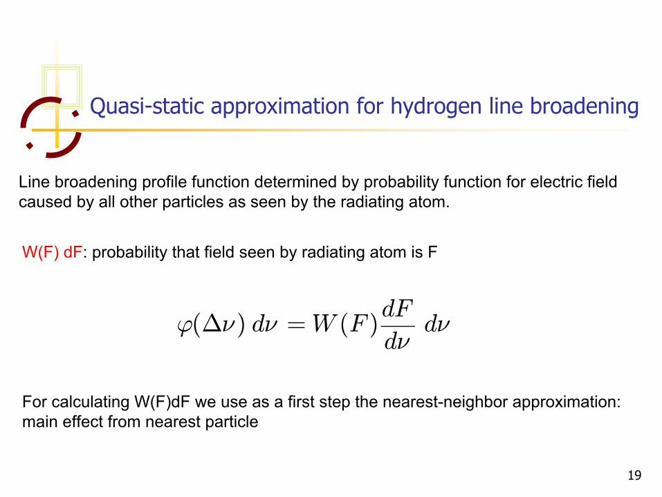
Quasi-static approximation for hydrogen line broadening

Line broadening profile function determined by probability function for electric field caused by all other particles as seen by the radiating atom.

W(F) dF: probability that field seen by radiating atom is F

For calculating W(F)dF

we use as a first step the nearest-neighbor approximation: main effect from nearest particle

ϕ(∆ν) dν =W (F )dF

dνdν

20

Quasi-static approximation – nearest neighbor approximation

assumption: main effect from nearest particle (F ~ 1/r2)

we need to calculate the probability that nearest neighbor is in

the distance range (r,r+dr) = probability that none is at distance < r and one is in (r,r+dr)

relative probability for particle in shell (r,r+dr) N: total uniform particle densityprobability for no particle in (0,r)

Integral equation for W(r) differentiating

differential equation

Normalized solution

Differential equation

21

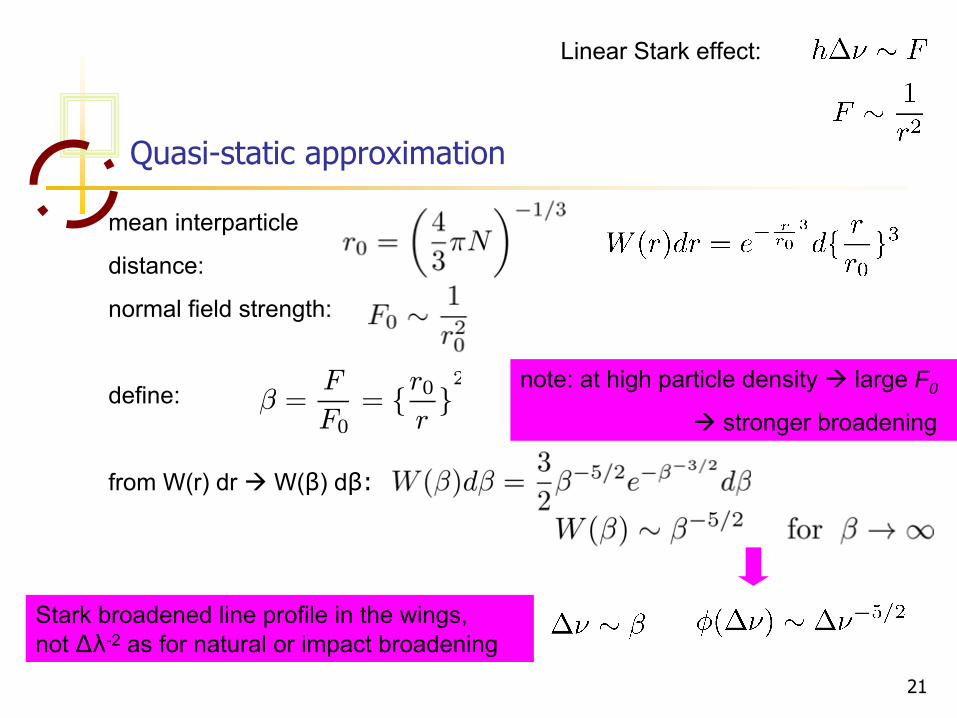
Quasi-static approximation

mean interparticle

distance:

normal field strength:

define:

from W(r) dr

W(β) dβ:

Stark broadened line profile in the wings, not Δλ-2

as for natural or impact broadening

note: at high particle density large F0

stronger broadeningβ =

F

F0= r0

r2

Linear Stark effect:

22

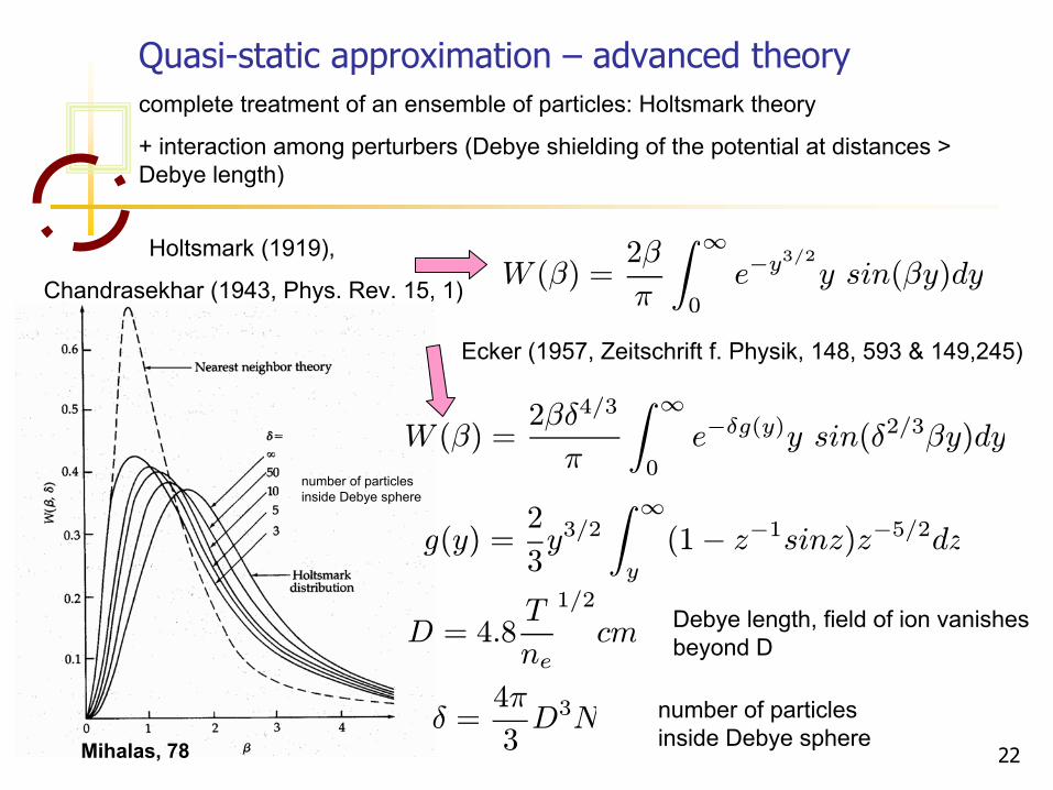
Quasi-static approximation –

advanced theorycomplete treatment of an ensemble of particles: Holtsmark

theory

+ interaction among perturbers

(Debye shielding of the potential at distances > Debye length)

number of particles inside Debye sphere

W (β) =2β

π

Z ∞

0

e−y3/2

y sin(βy)dyHoltsmark

(1919),

Chandrasekhar (1943, Phys. Rev. 15, 1)

W (β) =2βδ4/3

π

Z ∞

0

e−δg(y)y sin(δ2/3βy)dy

g(y) =2

3y3/2

Z ∞

y

(1− z−1sinz)z−5/2dz

δ =4π

3D3N

D = 4.8T

ne

1/2

cm

number of particles inside Debye sphere

Debye length, field of ion vanishes beyond D

Ecker

(1957, Zeitschrift

f. Physik, 148, 593 & 149,245)

Mihalas, 78

23

3. Doppler broadening

radiating atoms have thermal velocity

Maxwellian distribution:

Doppler effect: atom with velocity v emitting at frequency , observed at frequency :

ν0 = ν − νv cos θ

c

P (vx, vy , vz ) dvxdvydvz =³ m

2πkT

´3/2e−

m2kT (v

2x+v

2y+v

2z) dvxdvydvz

24

Doppler broadening

Define the velocity component along the line of sight:

The Maxwellian

distribution for this component is:

P (ξ) dξ =1

π1/2ξ0e−¡

ξξ0

¢2dξ

ξ0 = (2kT/m)1/2 thermal velocity

ν0 = ν − νξ

c

if v/c

<<1 line center

∆ν = ν0 − ν = −νξc= −[(ν − ν0) + ν0 ]

ξ

c≈ −ν0 ξ

c

if we observe at v, an atom with velocity component ξ

absorbs at ν′

in its frame

25

Doppler broadening

line profile for v = 0

profile for v ≠

0

ϕR(ν − ν0) =⇒ ϕR(ν0 − ν0) = ϕ(ν − ν0− ν0ξ

c)

New line profile: convolution

ϕnew(ν − ν0) =

∞Z−∞

ϕ(ν − ν0 − ν0ξ

c) P (ξ) dξ

profile function in rest frame

velocity distribution function

26

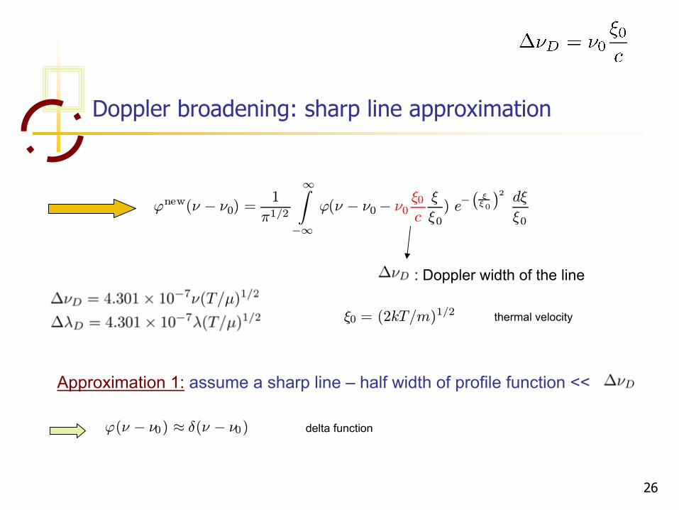
Doppler broadening: sharp line approximation

: Doppler width of the line

ϕnew(ν − ν0) =1

π1/2

∞Z−∞

ϕ(ν − ν0− ν0ξ0c

ξ

ξ0) e−

¡ξξ0

¢2 dξξ0

ξ0 = (2kT/m)1/2 thermal velocity

Approximation 1:

assume a sharp line –

half width of profile function <<

ϕ(ν − ν0) ≈ δ(ν − ν0) delta function

27

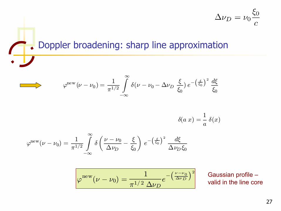
Doppler broadening: sharp line approximation

ϕnew (ν − ν0) =1

π1/2

∞Z−∞

δ(ν − ν0−∆νD ξ

ξ0) e−

¡ξξ0

¢2 dξξ0

δ(a x) =1

aδ(x)

ϕnew(ν − ν0) =1

π1/2

∞Z−∞

δ

µν − ν0∆νD

− ξ

ξ0

¶e−¡

ξξ0

¢2 dξ

∆νD ξ0

ϕnew(ν − ν0) =1

π1/2 ∆νDe−¡ν−ν0∆νD

¢2 Gaussian profile –

valid in the line core

28

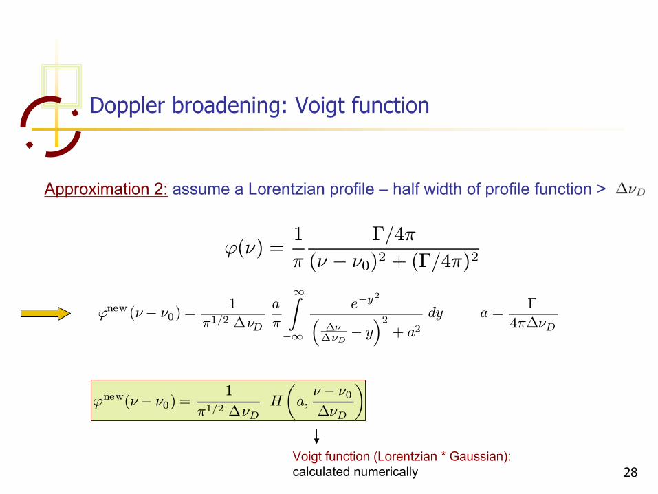
Doppler broadening: Voigt function

Approximation 2:

assume a Lorentzian

profile –

half width of profile function >

ϕnew (ν− ν0) =1

π1/2 ∆νD

a

π

∞Z−∞

e−y2³

∆ν∆νD

− y´2+ a2

dy a =Γ

4π∆νD

ϕnew(ν− ν0) =1

π1/2 ∆νDH

µa,

ν− ν0∆νD

¶

Voigt function (Lorentzian

* Gaussian): calculated numerically

ϕ(ν) =1

π

Γ/4π

(ν − ν0)2 + (Γ/4π)2

29

Voigt function: core Gaussian, wings Lorentzian

normalization:∞Z

−∞H(a, v) dv =

√π

usually α

<<1

max at v=0:

H(α,v=0) ≈

1-α

~ Gaussian ~ Lorentzian

Unsoeld, 68

30

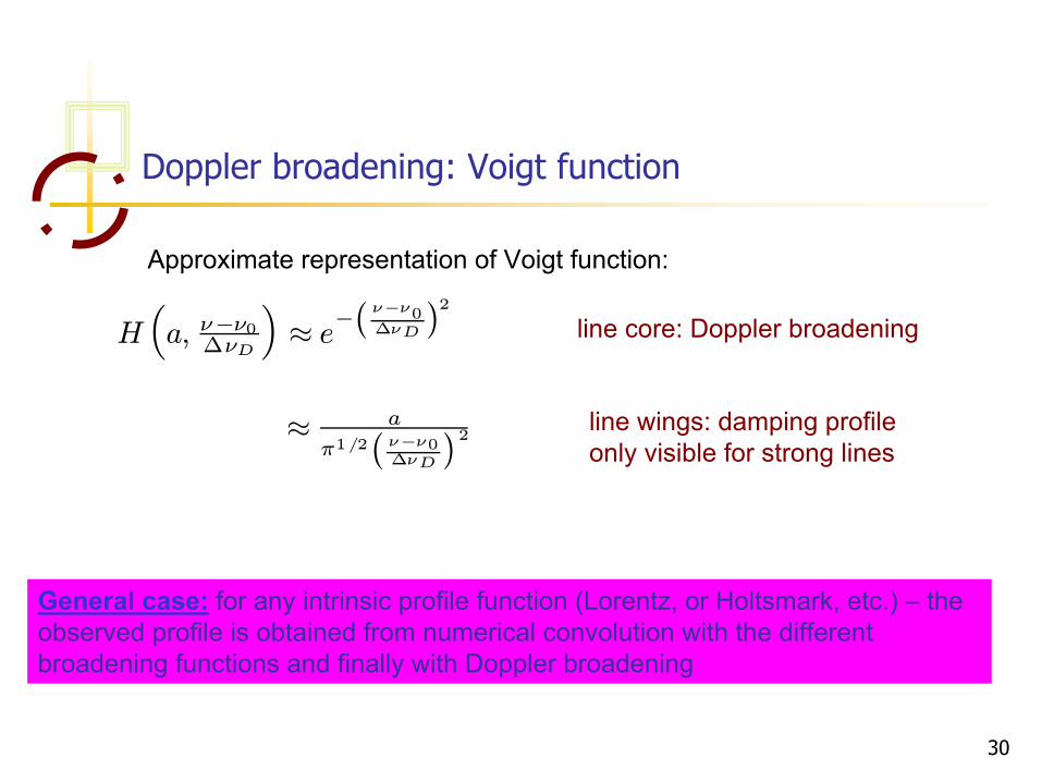
Doppler broadening: Voigt function

Approximate representation of Voigt function:

line core: Doppler broadening

line wings: damping profile only visible for strong lines

General case:

for any intrinsic profile function (Lorentz, or Holtsmark, etc.) –

the observed profile is obtained from numerical convolution with the

different broadening functions and finally with Doppler broadening

H³a, ν−ν0∆νD

´≈ e−

¡ν−ν0∆νD

¢2≈ a

π1/2¡ν−ν0∆νD

¢2

31

General case: two broadening mechanisms

two broadening functions representing

two broadening mechanisms

Resulting broadening function is convolution of the two individual broadening functions

32

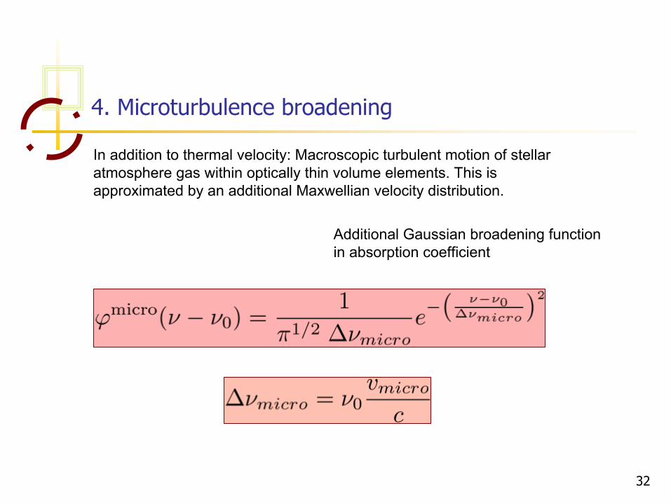
4. Microturbulence

broadening

In addition to thermal velocity: Macroscopic turbulent motion of

stellar atmosphere gas within optically thin volume elements. This is approximated by an additional Maxwellian

velocity distribution.

Additional Gaussian broadening function in absorption coefficient

33

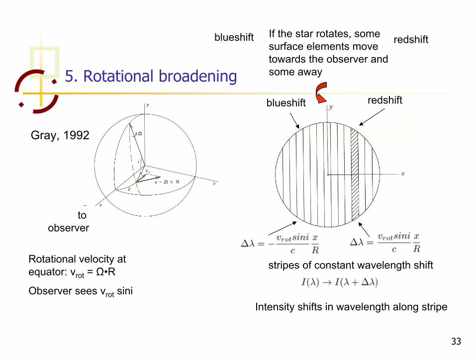
5. Rotational broadening

If the star rotates, some surface elements move towards the observer and some away

to observer

Rotational velocity at equator: vrot

= Ω•R

Observer sees vrot

sini

redshiftblueshift

stripes of constant wavelength shift

Intensity shifts in wavelength along stripe

Gray, 1992

blueshift redshift

34

stellar spectroscopy uses mostly normalized spectra Fλ

/ Fcontinuum

Rotation and observed line profile

integral over stellar disk towards observer, also

integral over all solid angles for one surface element

observed stellar line profile

Sprin

g 20

13

35

M33 A supergiant Keck (ESI)

U, Urbaneja, Kudritzki, 2009, ApJ

740, 1120

Fλ

/Fcontinuum

36

stellar spectroscopy uses mostly normalized spectra Fλ

/ Fcontinuum

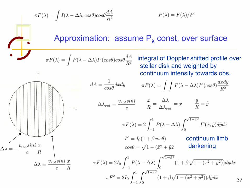
Rotation changes integral over stellar surface

integral over stellar disk towards observer

observed stellar line profile

Correct treatment by numerical integral over stellar surface with intensity calculated by model atmosphere

Gray, 1992

37

Approximation: assume Pλ

const. over surface

integral of Doppler shifted profile over stellar disk and weighted by continuum intensity towards obs.

continuum limb darkening

38

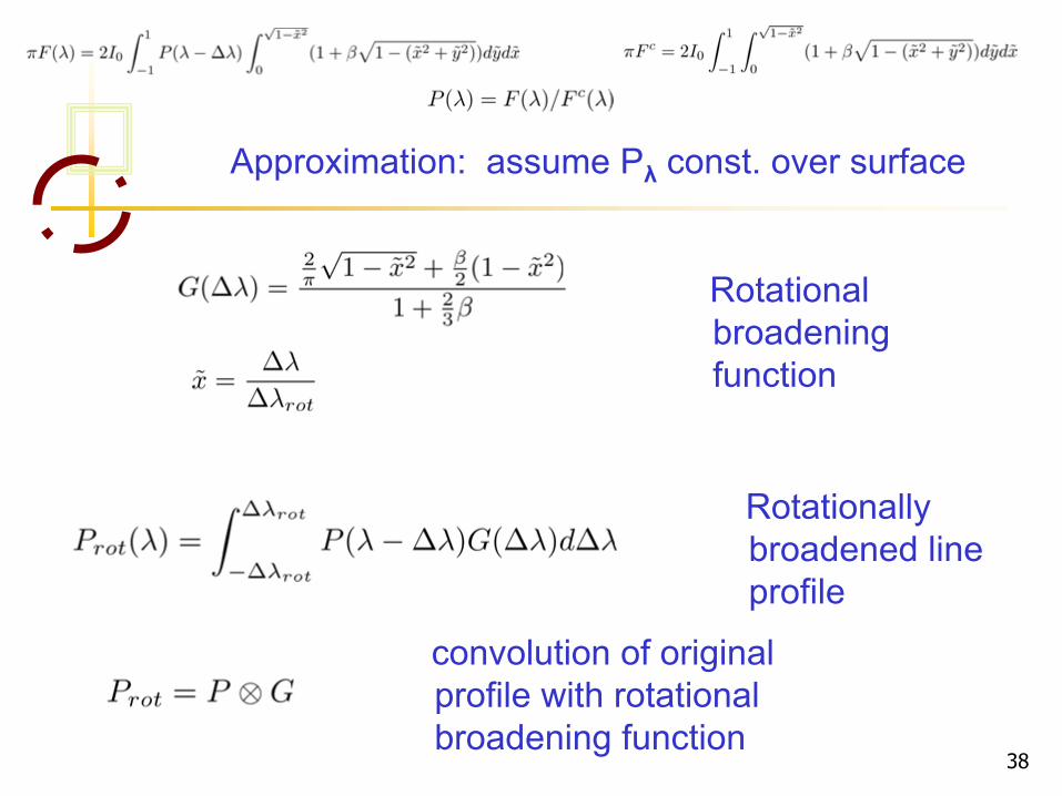
Approximation: assume Pλ

const. over surface

Rotational broadening function

Rotationally broadened line profile

convolution of original profile with rotational broadening function

39

Rotational broadening

Note: Rotational line broadening is not caused by physical processes affecting the absorption coefficient.

It is not the result of radiative

transfer.

It is caused by the macroscopic motion of the stellar surface elements and the Doppler-effect.

40

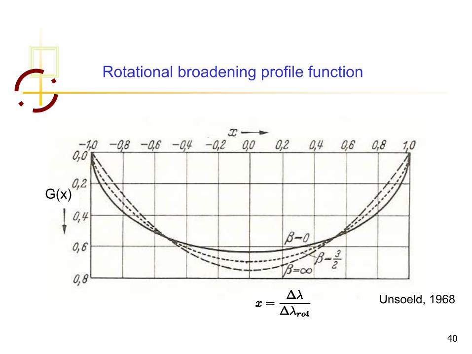
Rotational broadening profile function

G(x)

Unsoeld, 1968

41

Rotationally broadened line profiles

v sini km/s

Note: rotation does not change equivalent width!!!

Gray, 1992

42

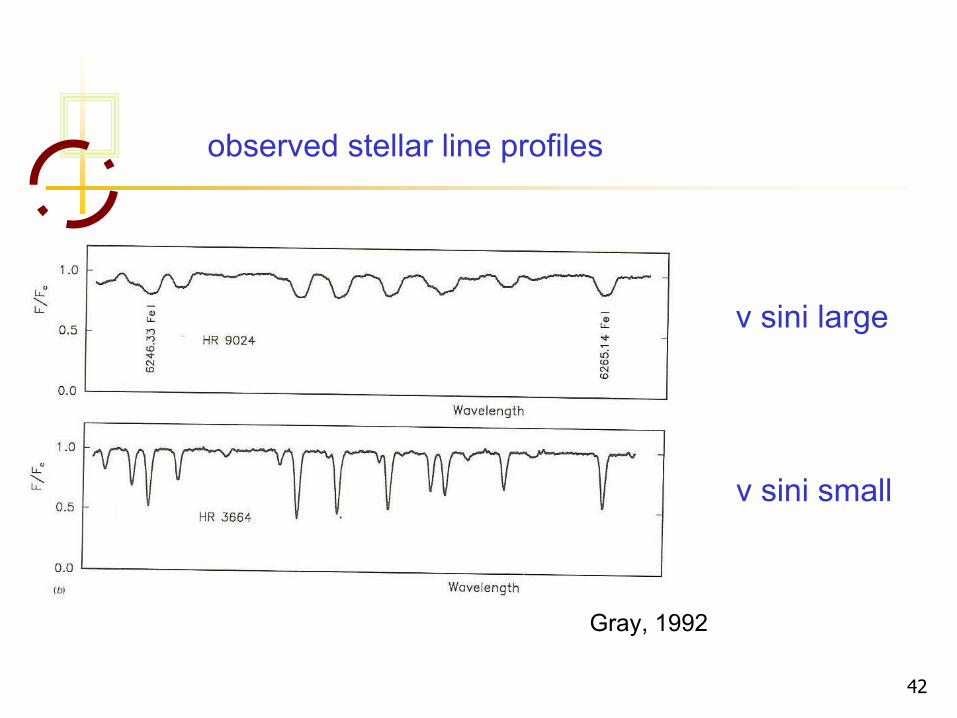
observed stellar line profiles

v sini

large

v sini

small

Gray, 1992

43

Rotationally broadened line profiles

v sini km/s

Note: rotation does not change equivalent width!!!

Gray, 1992

44

observed stellar line profiles

θ

Car, B0V vsini~250 km/s

Schoenberner, Kudritzki

et al. 1988

45

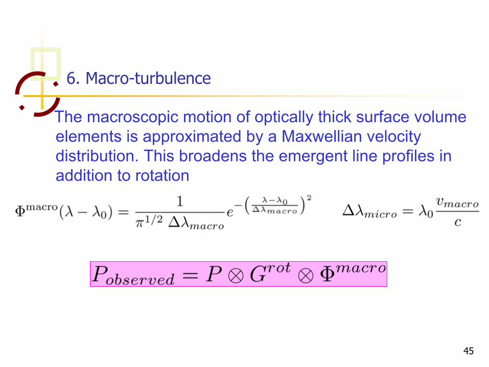
6. Macro-turbulence

The macroscopic motion of optically thick surface volume elements is approximated by a Maxwellian

velocity

distribution. This broadens the emergent line profiles in addition to rotation

46

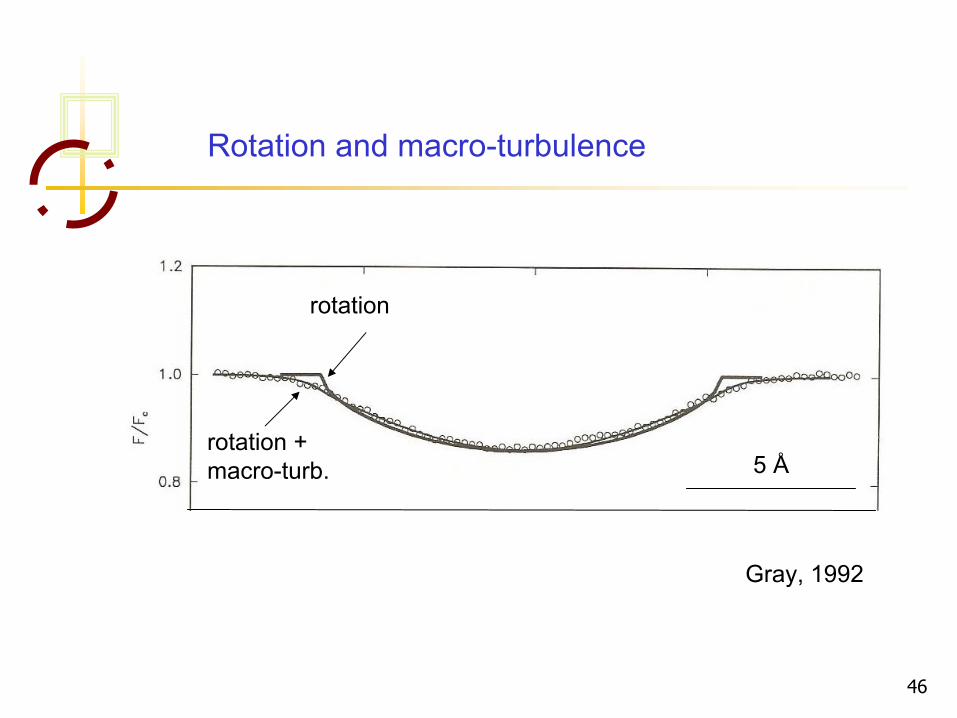
Rotation and macro-turbulence

Gray, 1992

5 Å

rotation

rotation +macro-turb.

47

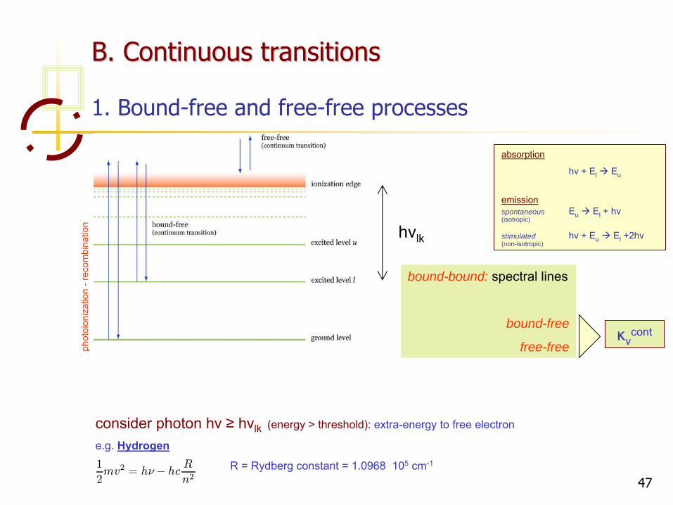
B. Continuous transitionsB. Continuous transitions

1. Bound-free and free-free processes

hνlk

consider photon hν ≥ hνlk

(energy > threshold): extra-energy to free electron

e.g. Hydrogen

R = Rydberg

constant = 1.0968 105

cm-1

absorption

hν

+ El

Eu

emissionspontaneous Eu

El + hν(isotropic)

stimulated hν + Eu

El +2hν(non-isotropic)

phot

oion

izat

ion

-rec

ombi

natio

n

bound-bound: spectral lines

bound-free

free-freeκνcont

1

2mv2 = hν− hc R

n2

48

b-f

and f-f

processes

l continuum Wavelength (A) Edge

1 continuum 912 Lyman

2 continuum 3646 Balmer

3 continuum 8204 Paschen

4 continuum 14584 Brackett

5 continuum 22790 Pfund

Hydrogen

49

b-f

and f-f

processes

for hydrogenic

ions

Gaunt factor ≈

1

for H: σ0

= 7.9 10-18

n cm2

νl

= 3.29 1015

/ n2

Hz

-

for a single transition

-

for all transitions:

κb−fν = nl σlk(ν)

κb− fν =X

elements,ions

Xl

nl σlk(ν)

Kramers

1923

absorption per particle

σlk(ν) = σ0(n)³νlν

´3gbf (ν)

Gray, 92

50

b-f

and f-f

processes

for non-H-like atoms no ν-3

dependence

peaks at resonant frequencies

free-free absorption much smaller

peaks increase with n:

σb-fn (ν) = 2.815× 1029Z 4

n5ν3gbf (ν)

late A

late B

hνn = E∞ − En = 13.6/n2eV

=⇒ ν−3 → n

6

Gray, 92

51

b-f

and f-f

processes

Hydrogen dominant continuous absorber in B, A & F stars (later stars H-)

Energy distribution strongly modulated at the edges:

Vega

Balmer

Paschen

Brackett

52

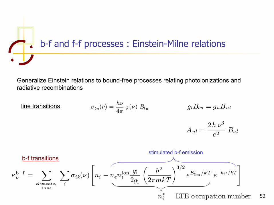
b-f

and f-f

processes : Einstein-Milne relations

Generalize Einstein relations to bound-free processes relating photoionizations

and radiative

recombinations

σlu(ν) =hν

4πϕ(ν) Bluline transitions glBlu = guBul

Aul =2h ν3

c2Bul

b-f

transitions

κb−fν =X

elements,ions

Xi

σik(ν)

"ni − nenIon1

gi2g1

µh2

2πmkT

¶3/2eE

iIon /kT e−hν/kT

#

n∗i LTE occupation number

stimulated b-f

emission

53

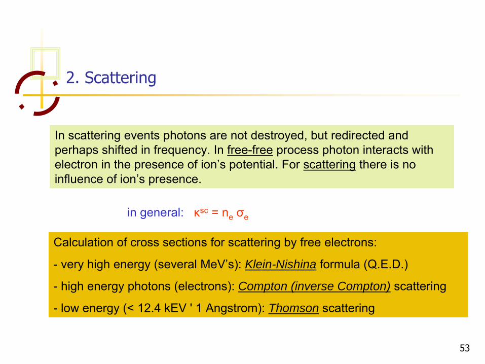
2. Scattering

In scattering events photons are not destroyed, but redirected and perhaps shifted in frequency. In free-free

process photon interacts with electron in the presence of ion’s potential. For scattering

there is no influence of ion’s presence.

Calculation of cross sections for scattering by free electrons:

-

very high energy (several MeV’s): Klein-Nishina formula (Q.E.D.)

-

high energy photons (electrons): Compton (inverse Compton) scattering

-

low energy (< 12.4 kEV

'

1 Angstrom): Thomson scattering

in general:

κsc

= ne

σe

54

Thomson scattering

THOMSON

SCATTERING: important source of opacity in hot OB stars

independent of frequency, isotropic

Approximations:

-

angle averaging done, in reality: σe

σe

(1+cos2

θ) for single scattering

-

neglected velocity distribution and Doppler shift (frequency-dependency)

σe =8π

3r20 =

8π

3

e4

m2e c4= 6.65× 10−25cm2

55

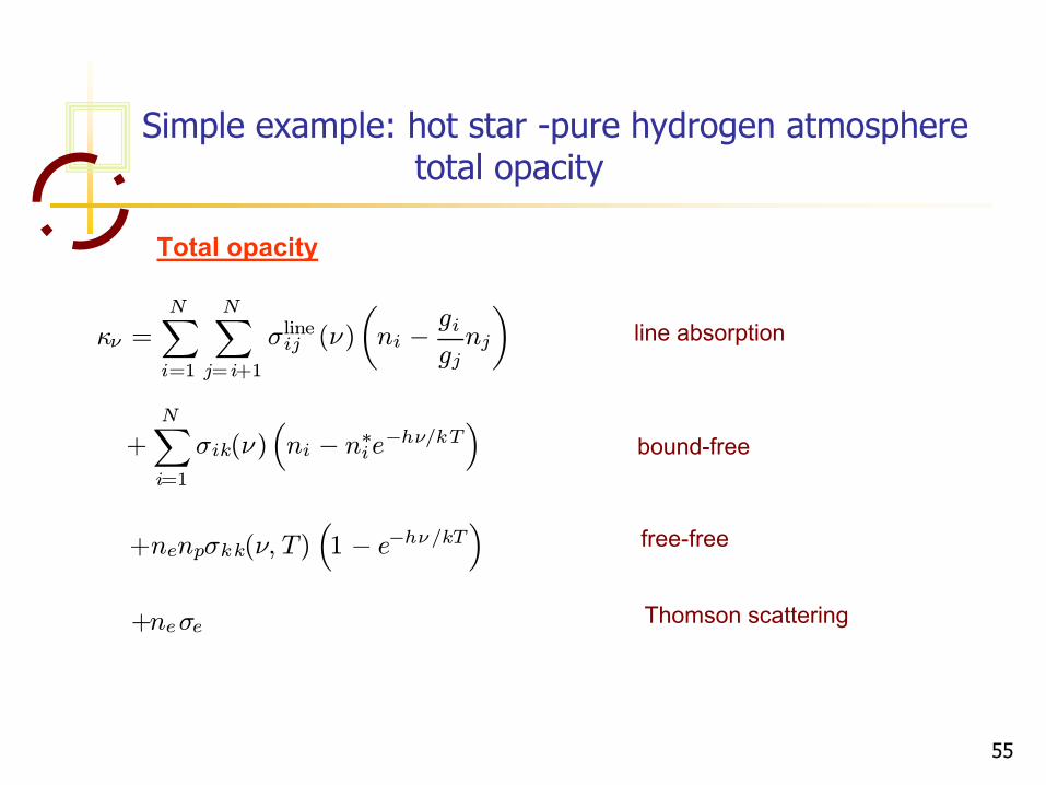
Simple example: hot star -pure hydrogen atmosphere total opacity

Total opacity

κν =NXi=1

NXj= i+1

σlineij (ν)

µni − gi

gjnj

¶

+NXi=1

σik(ν)³ni − n∗ie−hν/kT

´

+nenpσkk(ν, T )³1 − e−hν/kT

´+neσe

line absorption

bound-free

free-free

Thomson scattering

56

Total emissivity

line emission

bound-free

free-free

Thomson scattering

²ν =2hν3

c2

NXi=1

NXj=i+1

σ lineij (ν)gigjnj

+2hν3

c2

NXi=1

n∗iσik(ν)e−hν/kT

+2hν3

c2nenpσkk(ν, T)e

−hν/kT

+neσe Jν

Simple example: hot star -pure hydrogen atmosphere total emissivity

57

Rayleigh scattering –

important in cool stars

RAYLEIGH

SCATTERING: line absorption/emission of atoms and molecules far from resonance frequency: ν

<< ν0

from classical expression of cross section for oscillators:

σ(ω) = fijσkl(ω) = fij σeω4

(ω2 − ω2ij)2+ ω2γ2

for ω << ωij σ(ω) ≈ fij σe ω4

ω4ij + ω2γ2

for γ << ωij σ(ω) ≈ fij σe ω4

ω4ij

σ(ω) ∼ ω4 ∼ λ−4

important in cool G-K stars

for strong lines (e.g. Lyman series when H is neutral) the λ-4

decrease in the far wings can be important in the optical

58

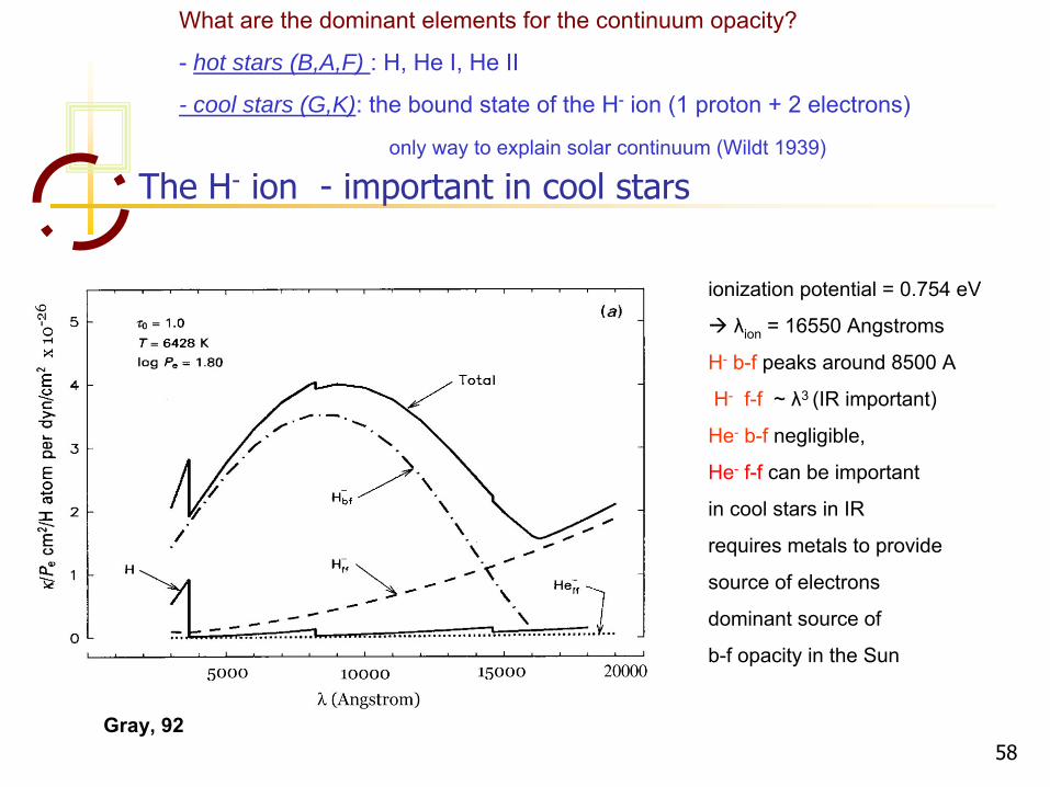
The H-

ion -

important in cool stars

What are the dominant elements for the continuum opacity?

-

hot stars (B,A,F) : H, He I, He II

- cool stars (G,K): the bound state of the H-

ion (1 proton + 2 electrons)

only way to explain solar continuum (Wildt

1939)

ionization potential = 0.754 eV

λion

= 16550 Angstroms

H-

b-f

peaks around 8500 A

H-

f-f

~ λ3 (IR important)

He-

b-f

negligible,

He-

f-f

can be important

in cool stars in IR

requires metals to provide

source of electrons

dominant source of

b-f

opacity in the Sun

Gray, 92

59

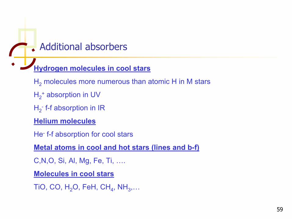
Additional absorbers

Hydrogen molecules in cool stars

H2

molecules more numerous than atomic H in M stars

H2+

absorption in UV

H2-

f-f

absorption in IR

Helium molecules

He-

f-f

absorption for cool stars

Metal atoms in cool and hot stars (lines and b-f)

C,N,O, Si, Al, Mg, Fe, Ti, ….

Molecules in cool stars

TiO, CO, H2

O, FeH, CH4

, NH3

,…

60

Examples of continuous absorption coefficients

Teff

= 5040 K B0: Teff

= 28,000 K

Unsoeld, 68

61

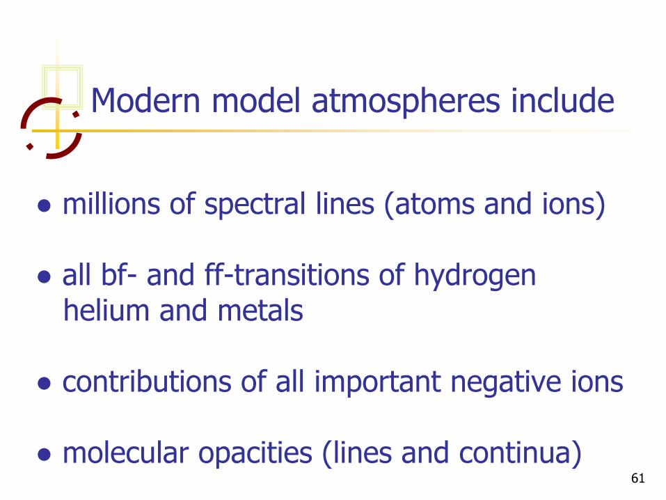
Modern model atmospheres include

millions of spectral lines (atoms and ions)

all bf-

and ff-transitions of hydrogen helium and metals

contributions of all important negative ions

molecular opacities (lines and continua)

Con

cepc

ion

2007

62

complex atomic models for O-stars (Pauldrach et al., 2001)

AWAP 05/19/05 63

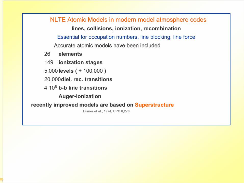
NLTENLTE

AtomicAtomic

ModelsModels

in modern model atmosphere codesin modern model atmosphere codeslines, collisions,

ionization, recombination Essential for occupation numbers, line blocking, line force

Accurate atomic models have been includedAccurate atomic models have been included26

elements149

ionization stages5,000 levels ( + 100,000

)20,000diel. rec. transitions4 106

b-b

line transitionsAuger-ionization

recently improved models are based onrecently improved models are based on

SuperstructureSuperstructureEisner et al., 1974, CPC 8,270

Con

cepc

ion

2007

64

65

Recent Improvements on Atomic Data

•

requires solution of Schrödinger equation

for N-electron system

•

efficient technique:R-matrix method in CC approximation

•

Opacity Project Seaton et al. 1994, MNRAS, 266, 805

•

IRON Project Hummer et al. 1993, A&A, 279, 298

accurate radiative/collisional datato 10% on the mean

66

Confrontation with Reality

Photoionization Electron Collision

Nahar 2003, ASP Conf. Proc.Ser. 288, in press Williams 1999, Rep. Prog. Phys., 62, 1431

high-precision atomic data

67

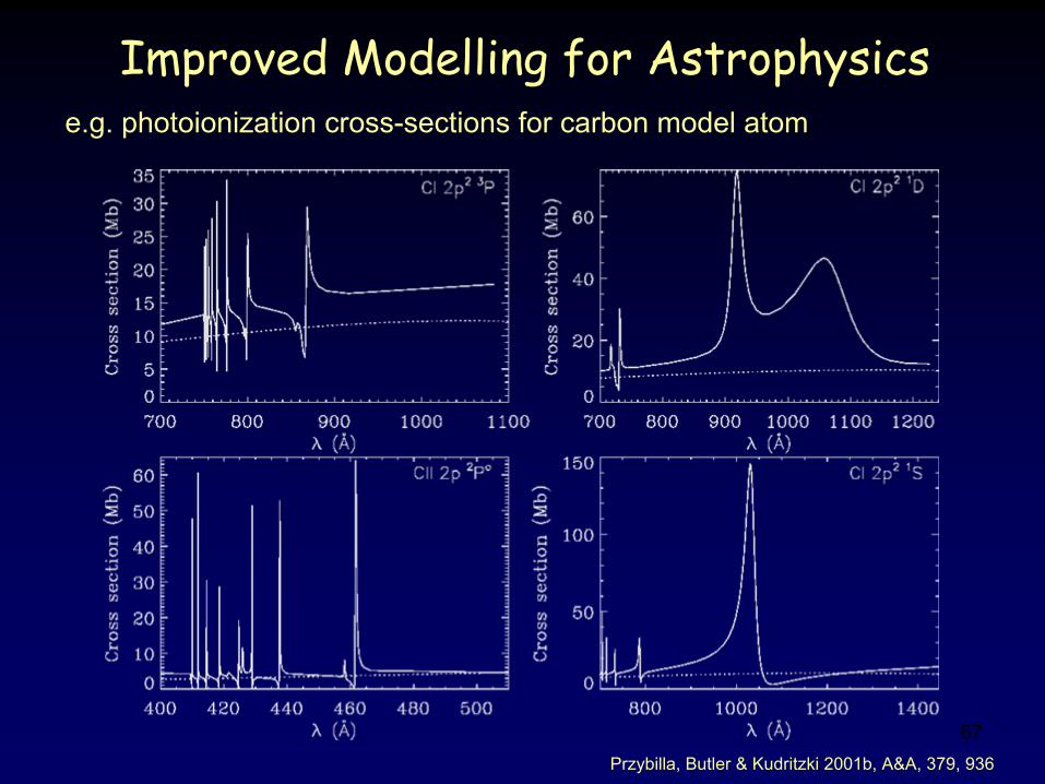
Improved Modelling for Astrophysics

Przybilla, Butler & Kudritzki 2001b, A&A, 379, 936

e.g. photoionization cross-sections for carbon model atom

68

Bergemann, Kudritzki

et al., 2012

Red supergiants, NLTE model atom for FeI

69

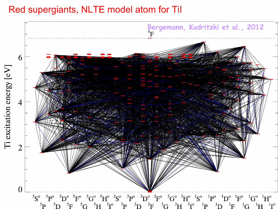
Red supergiants, NLTE model atom for TiI

Bergemann, Kudritzki

et al., 2012

70

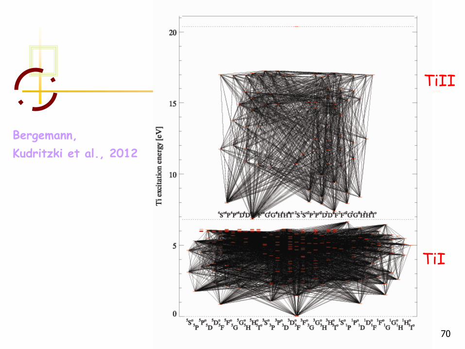
TiI

TiII

Bergemann, Kudritzki

et al., 2012

US

M 2

011

71

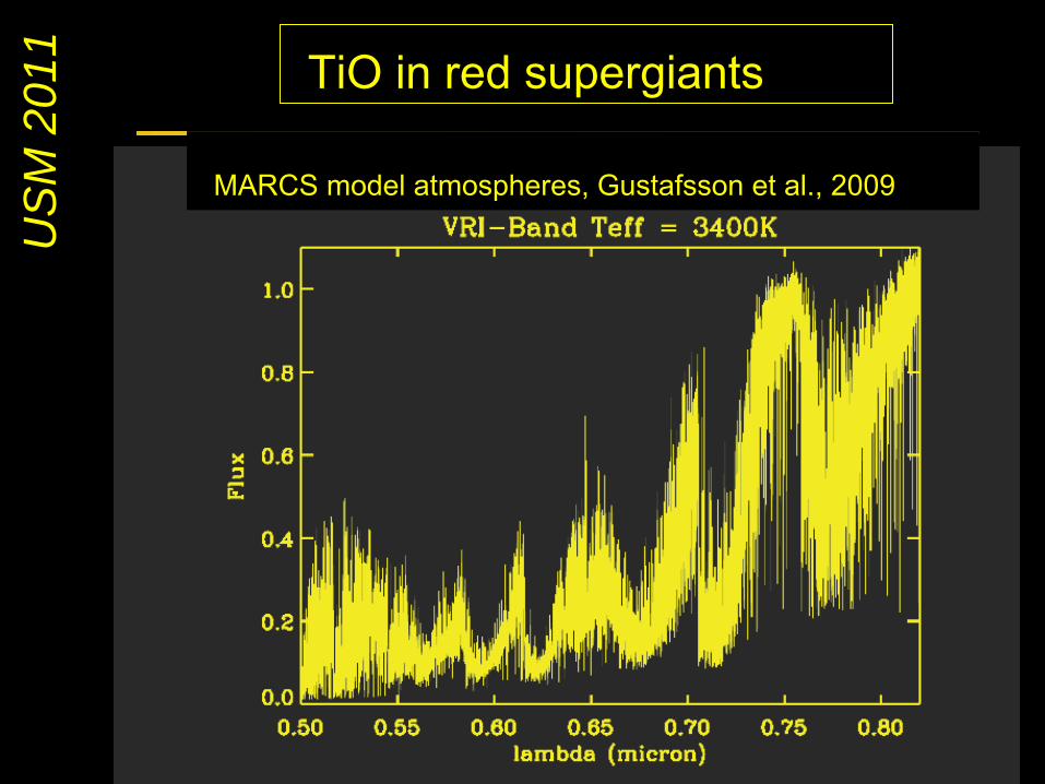
TiO

in red supergiants

MARCS model atmospheres, Gustafsson

et al., 2009

US

M 2

011

72

A small change in carbon abundances…

MARCS modelatmospheres

TiO

in red supergiants

73

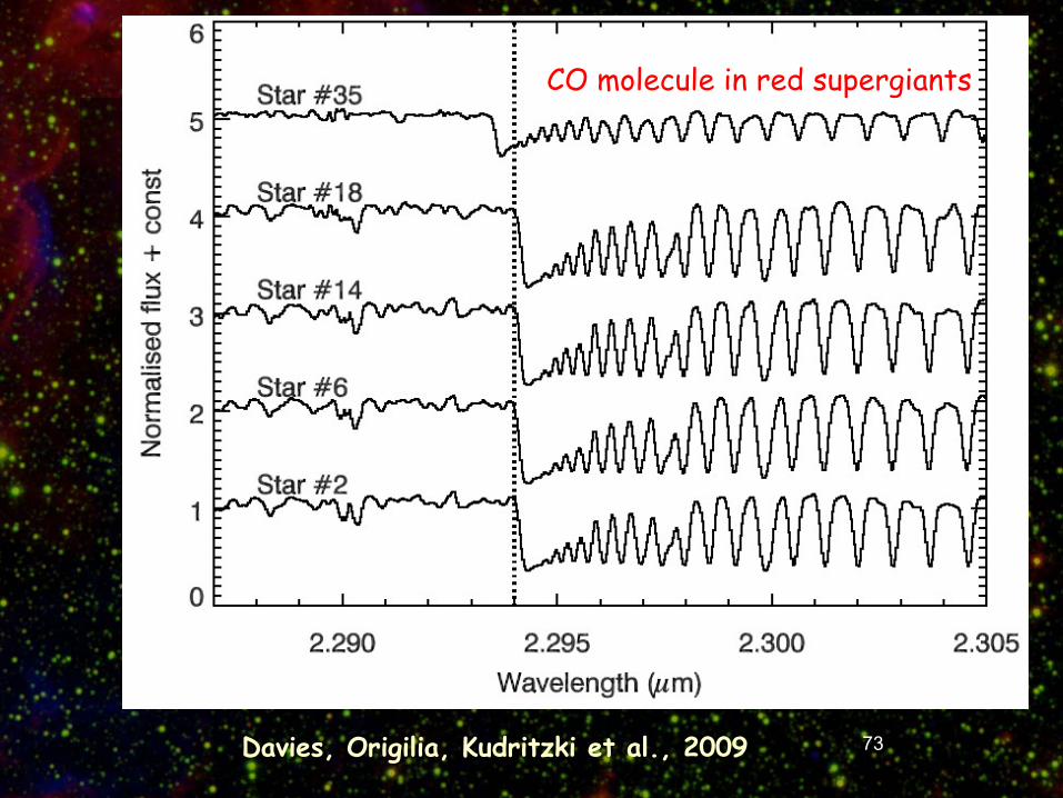
The Scutum RSG clusters

CO molecule in red supergiants

Davies, Origilia, Kudritzki

et al., 2009

74

Rayner, Cushing, Vacca, 2009: molecules in Brown Dwarfs

75

Exploring the substellar temperature regime down to ~550KBurningham et al. (2009)

T9.0 ~ 550K

T8.5 ~ 700K

Jupiter