Embed Size (px)
Citation preview

5 Analysis of stress and strain
5.1 Introduction
Up to the present we have confined our attention to considerations of simple direct and shearing stresses. But in most practical problems we have to deal with combinations of these stresses.
The strengths and elastic properties of materials are determined usually by simple tensile and compressive tests. How are we to make use of the results of such tests when we know that stress in a given practical problem is compounded from a tensile stress in one direction, a compressive stress in some other direction, and a shearing stress in a third direction? Clearly we cannot make tests of a material under all possible combinations of stress to determine its strength. It is essential, in fact, to study stresses and strains in more general terms; the analysis which follows should be regarded as having a direct and important bearing on practical strength problems, and is not merely a display of mathematical ingenuity.
5.2 Shearing stresses in a tensile test specimen
A long uniform bar, Figure 5.1, has a rectangular cross-section of area A . The edges of the bar are parallel to perpendicular axes Ox, QY, Oz. The bar is uniformly stressed in tension in the x- direction, the tensile stress on a cross-section of the bar parallel to Ox being ox. Consider the stresses acting on an inclined cross-section of the bar; an inclined plane is taken at an angle 0 to the yz-plane. The resultant force at the end cross-section of the bar is acting parallel to Ox.
P = Ao,
Figure 5.1 Stresses on an inclined plane through a tensile test piece.
For equilibrium the resultant force parallel to Ox on an inclined cross-section is also P = Ao,. At the inclined cross-section in Figure 5.1, resolve the force Ao, into two components-one

Shearing stresses in a tensile test specimen 95
perpendicular, and the other tangential, to the inclined cross-section, the latter component acting parallel to the xz-plane. These two components have values, respectively, of
Ao, cos 0 and Ao, sin 0
The area of the inclined cross-section is
A sec 0
so that the normal and tangential stresses acting on the inclined cross-section are
A o , sin0 A sec0
T = = o x cos0 sin0
o is the direct stress and T the shearing stress on the inclined plane. It should be noted that the stresses on an inclined plane are not simply the resolutions of ox perpendicular and tangential to that plane; the important point in Figure 5.1 is that the area of an inclined cross-section of the bar is different from that of a normal cross-section. The shearing stress T may be written in the form
T = cr, case sine = + o x sin28
At 0 = 0" the cross-section is perpendicular to the axis of the bar, and T = 0; T increases as 0 increases until it attains a maximum of !4 ox at 6 = 45 " ; T then diminishes as 0 increases further until it is again zero at 0 = 90". Thus on any inclined cross-section of a tensile test-piece, shearing stresses are always present; the shearing stresses are greatest on planes at 45 " to the longitudinal axis of the bar.
Problem 5.1 A bar of cross-section 2.25 cm by 2.25 cm is subjected to an axial pull of 20 kN. Calculate the normal stress and shearing stress on a plane the normal to which makes an angle of 60" with the axis of the bar, the plane being perpendicular to one face of the bar.
Solution
We have 0 = 60", P = 20 kN and A = 0.507 xlO-' m2. Then
o x = 2o lo3 = 39.4 m / m 2 0.507 x
The normal stress on the oblique plane is
o = o x cos2 60' = -$ = 9.85MNIm'

96 Analysis of stress and strain
The shearing stress on the oblique plane is
fo,sin120° = f ( 3 9 . 4 ~ 1 0 6 ) g = 17.05MN/m2
5.3 Strain figures in mild steel; Luder's lines
If a tensile specimen of mild steel is well polished and then stressed, it will be found that, when the specimen yields, a pattern of fine lines appears on the polished surface; these lines intersect roughly at right-angles to each other, and at 45" approximately to the longitudinal axis of the bar; these lines were first observed by Luder in 1854. Luder's lines on a tensile specimen of mild steel are shown in Figure 5.2. These strain figures suggest that yielding of the material consists of slip along the planes of greatest shearing stress; a single line represents a slip band, containing a large number of metal crystals.
Figure 5.2 Liider's lines in the yielding of a steel bar in tension.
5.4 Failure of materials in compression
Shearing stresses are also developed in a bar under uniform compression. The failure of some materials in compression is due to the development of critical shearing stresses on planes inclined to the direction of compression. Figure 5.3 shows two failures of compressed timbers; failure is due primarily to breakdown in shear on planes inclined to the direction of compression.

General two-dimensional stress system 97
Figure 5.3 Failures of compressed specimens of timber, showing breakdown of the material in shear.
5.5 General two-dimensional stress system
A two-dimensional stress system is one in which the stresses at any point in a body act in the same plane. Consider a thin rectangular block of material, abcd, two faces of which are parallel to the xy-plane, Figure 5.4. A two-dimensional state of stress exists if the stresses on the remaining four faces are parallel to the xy-plane. In general, suppose theforces acting on the faces are P, Q, R, S, parallel to the xy-plane, Figure 5.4. Each of these forces can be resolved into components P,, P, etc., Figure 5.5. The perpendicular components give rise to direct stresses, and the tangential components to shearing stresses.
The system of forces in Figure 5.5 is now replaced by its equivalent system of stresses; the rectangular block of Figure 5.6 is in uniform state of two-dimensional stress; over the two faces parallel to Ox are direct and shearing stresses oy and T,~, respectively. The hckness is assumed to be 1 unit of length, for convenience, the other sides having lengths a and b. Equilibrium of the block in the x- andy-directions is already ensured; for rotational equilibrium of the block in the xy- plane we must have
[ T ~ (a x l)] x b = [ T , ~ (b x l)] x a

98 Analysis of stress and strain
Figure 5.4 Resultant force acting on the faces Figure 5.5 Components of resultant forces parallel to 0, and 0,. of a ‘twodimensional’ rectangular block.
ThUS ( U b ) T v = ( U b ) T y x
or ‘IT = 7yx (5.3)
Then the shearing stresses on perpendicular planes are equal and complementary as we found in the simpler case of pure shear in Section 3.3.
Figure 5.6 General two-dimensional Figure 5.7 Stresses on an inclined state of stress. plane in a two-dimensional stress system.
5.6 Stresses on an inclined plane
Consider the stresses acting on an inclined plane of the uniformly stressed rectangular block of Figure 5.6; the inclined plane makes an angle 6 with O,, and cuts off a ‘triangular’ block, Figure 5.7. The length of the hypotenuse is c, and the thickness of the block is taken again as one unit of length, for convenience. The values of direct stress, 0, and shearing stress, T, on the inclined plane are found by considering equilibrium of the triangular block. The direct stress acts along the normal to the inclined plane. Resolve the forces on the three sides of the block parallel to this

Stresses on an inclined plane 99
normal: then
a (c.i) = a, (c case case) + oy (c sine sine) + Tv (c case sine) + TV (c sine case)
This gives
0 = ox cos2 e + 0, Sin2 8 + 2T, sin e COS e (5.4)
Now resolve forces in a direction parallel to the inclined plane:
T. (C 1) = -0, (c case sine) + oY (c sine case) + Txy (c case case) - T ~ (c sine sine)
This gives
T = -0, case sine + oY sine case + Tv(COS2e - sin2e)
The expressions for a and T are written more conveniently in the forms:
a = %(ax + 0,) + %(ax - 0,) cos28 + T~ sin2e
T = -%(ax - oy) sin28 + T~ cos20
The shearing stress T vanishes when
that is, when
These may be written
(5.7)

100 Analysis of stress and strain
In a two-dimensional stress system there are thus two planes, separated by go", on which the shearing stress is zero. These planes are called theprincipalplanes, and the corresponding values of o are called the principal stresses. The direct stress ts is a maximum when
- - do - -(ox - a,,) sin28 + 2TT c o s ~ = o de
that is, when
2 5 w e = - ox - oy
which is identical with equation (5.8), defining the directions of the principal stresses; thus the principal stresses are also the maximum and minimum direct stresses in the material.
5.7 Values of the principal stresses
The directions of the principal planes are given by equation (5.8). For any two-dimensional stress system, in which the values of ox, cry and T~ are known, tan28 is calculable; two values of 8, separated by go", can then be found. The principal stresses are then calculated by substituting these vales of 8 into equation (5.6).
Alternatively, the principal stresses can be calculated more directly without finding the principal planes. Earlier we defined a principal plane as one on which there is no shearing stress; in Figure 5.8 it is assumed that no shearing stress acts on a plane at im angle 8 to QY.
Figure 5.8 A principal stress acting on an inclined plane; there is no shearing stress T associated with a principal stress o.
For equilibrium of the triangular block in the x-direction,
~ ( c case) - 0, (c case) = T~ (c sine)
and so o-o,= ~ , t a n e (5.10)

Maximum shearing stress
For equilibrium of the block in the y-direction
101
and thus
o - oy = T,COte (5.1 1)
On eliminating 8 between equations (5.10) and (5.1 1); by multiplying these equations together, we get
(0 - 0,) (o - oy) = T2xv
This equation is quadratic in o; the solutions are ~~
o, = + (ox + oy) + +,(crx - c r y ) 2 + 4 7 ~ = maximum principal stress
(5.12)
which are the values of the principal stresses; these stresses occur on mutually perpendicular planes.
5.8 Maximum shearing stress
The principal planes define directions of zero shearing stress; on some intermediate plane the shearing stress attains a maximum value. The shearing stress is given by equation (5.7); T attains a maximum value with respect to 0 when
i.e., when
The planes of maximum shearing stress are inclined then at 45" to the principal planes. On substituting this value of cot 28 into equation (5.7), the maximum numerical value of T is

102 Maximum shearing stress
Tm, = /[+(ox - 41' + [%I2 (5.13)
But from equations (5.12),
where o, and o2 are the principal stresses of the stress system. Then by adding together the two equations on the right hand side, we get
and equation (5.13) becomes
1 T"ax = T(0, - 0 2 ) (5.14)
The maximum shearing stress is therefore half the difference between the principal stresses of the system.
Problem 5.2 At a point of a material the two-dimensional stress system is defined by
ox = 60.0 MN/m2, tensile
oy = 45.0 MN/m2, compressive
T, = 37.5 MN/m2, shearing
where ox, o,,, 'I, refer to Figure 5.7. Evaluate the values and directions of the principal s&esses. What is the greatest shearing stress?
Solution
Now, we have
-Lo * ( +d y ) = + (60.0 - 45.0) = 7.5 MN/m'
+(ox - o Y ) = 4 (60.0 + 45.0) = 52.5 MN/m2

Mohr's circle of stress
Then, from equations (5.12),
oI = 7.5+ [ ( 5 2 5 ) 2 + (375)2]i = 7.5+64.4 = 71.9MN/m2
0 2 = 7.5 - [(525)2 + (375)2]' = 7.5 - 64.4 = -56.9MN/m2 I
103
From equation (5.8)
Thus,
28 = tar-' (0.714) = 35.5" or 215.5"
Then
€4 = 17.8" or 107.8'
From equation (5.14)
T , , , ~ = L(ol - 02) = 1(71.9+56.9) = 64.4 MN/m* 2 2
This maximum shearing stress occurs on planes at 45 " to those of the principal stresses.
5.9 Mohr's circle of stress
A geometrical interpretation of equations (5.6) and (5.7) leads to a simple method of stress analysis. Now, we have found already that
Take two perpendicular axes 00, &, Figure 5.9; on h s co-ordinate system set off the point having co-ordinates (ox, TJ and (o,,, - TJ, corresponding to the known stresses in the x- andy-directions. The line PQ joining these two points is bisected by the Oa axis at a point 0'. With a centre at 0', construct a circle passing through P and Q. The stresses o and T on a plane at an angle 8 to Oy are found by setting off a radius of the circle at an angle 28 to PQ, Figure 5.9; 28 is measured in a clockwise direction from 0' P.

104 Analysis of stress and strain
Figure 5.9 Mohr's circle of stress. The points P and Q correspond to the stress states (ox, rv) and (o,,, - rv) respectively, and are diametrically opposite;
the state of stress (0, r) on a plane inclined at an angle 0 to 9, is given by the point R.
The co-ordinates of the point R(o, T) give the direct and shearing stresses on the plane. We may write the above equations in the forms
o - Z(or 1 + o,,) = +(or - O , ) C O S ~ ~ + T~ sin20
-r = l(or-a,)sin2e-T,cos2e 2
Square each equation and add; then we have
[,-L(q+ 2 0 y ) r + T 2 = [+(ox- O.")l'+[.^l' (5.15)
Thus all corresponding values of o and T lie on a circle of radius
r +-oy) ] + T L
with its centre at the point (%[or + a,,], 0), Figure 5.9.
This circle defining all possible states of stress is known as Mohr's Circle ofstress; the principal stresses are defined by the points A and E, at which T = 0. The maximum shearing stress, which is given by the point C, is clearly the radius of the circle.
Problem 5.3 At a point of a material the stresses forming a two-dimensional system are shown in Figure 5.10. Using Mohr's circle of stress, determine the magnitudes and directions of the principal stresses. Determine also the value of the maximum shearing stress.

Mohr’s circle of stress 105
Figure 5.10. Stress at a point.
Solution
FromFigure 5.10, the shearing stresses acting in conjunction with (T, are counter-clockwise, hence, T~ is said to be positive on the vertical planes. Similarly, the shearing stresses acting in conjunction with T~ are clockwise, hence, T~ is said to be negative on the horizontal planes.
On the (T - T diagram of Figure 5.1 1, construct a circle with the line joining the point (ox, T ~ ) or (50,20) and the point ((T,,, - T ~ ) or (30,-20) as the diameter, as shown by A and B, respectively
Figure 5.11 Problem 5.3.
The principal stresses and their directions can be obtained from a scaled drawing, but we shall calculate (T,, (T, etc.
DA = 20 MPa OD = (3, = 50 MPa OG = cry = 30MPa

106 Analysis of stress and strain
= 40 MPa (OD + OG) - (50 + 30) 2 2
CD = OD - OC = 50 - 40 = 10MPa
o c = - -
A C ~ = CD' + D A ~
= I O 2 + 202
or AC = 22.36 MPa
crl = OE = OC + AC = 40 + 22.36
cr, = 62.36 MPa
o2 = OF = OC - AC
= 40 - 22.36
or c2 = 17.64 MPa
28 = tan-' (z) = tan-' (E) = 63.43'
:. 8 = 31.7" see below
Maximum shear stress = T~~ = AC = 22.36 MPa which occurs on planes at 45 O to those of the principal stresses.

Mohr’s circle of stress 107
At a point of a material the two-dimensional state of stress is shown in Figure 5.12. Determine o,, ozr 8 and T-
Problem 5.4
Figure 5.12 Stress at a p i n t .
Solution
On the o-T diagram of Figure 5.13, construct a circle with the line joining the point (o* T,) or (30, 20) to the point (cry, -7,) or (-10, -20), as the diameter, as shown by the points A and B respectively. It should be noted that T~ is positive on the vertical planes of Figure 5.12, as these shearing stresses are causing a counter-clockwise rotation; vice-versa for the shearing stresses on the horizontal planes.
Figure 5.13 Problem 5.4.
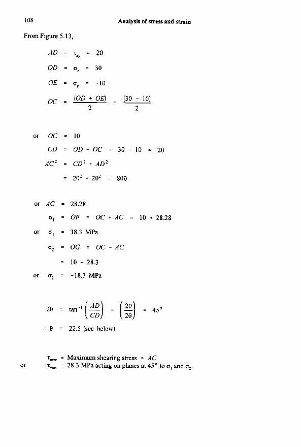
108 Analysis of stress and strain
From Figure 5.13,
AD = = 20
OD = ox = 30
OE = o,, = -10
oc = - (OD + OE) - (30 - 10) 2 2
or OC = 10
CD = OD - OC = 30 - 10 = 20
AC2 = CD2 + AD2
= 202 + 202 = 800
or AC = 28.28
o1 = OF = OC + AC = 10 + 28.28
or (rl = 38.3 MPa
ct = OG = OC - AC
= 10 - 28.3
or o2 = -18.3 MPa
:. 8 = 22.5 (see below)
T- = Maximushearingstress = AC L~ = 28.3 MPa acting on planes at 45" to o, and 02. or

Strains in an inclined direction 109
5.10 Strains in an inclined direction
For two-dimensional system of strains the direct and shearing strains in any direction are known if the dxect and shearing strains in two mutually perpendicular directions are given. Consider a rectangular element of material, OABC, in the xy-plane, Figure 5.14, it is required to find the direct and shearing strains in the direction of the diagonal OB, when the direct and shearing strains in the directions Ox, Oy are given. Suppose E, is the strain in the direction Ox, E, the strain in the direction Oy, and y, the shearing strain relative to Ox and Oy.
Figure 5.14 Strains in an inclined direction; strains in the directions 0, and 0, and defined by E,, E, and y,, lead to strains E , y along the inclined direction OB.
All the strains are considered to be small; in Figure 5.14, if the diagonal OB of the rectangle is taken to be of unit length, the sides OA, OB are of lengths sine, cos0, respectively, in which 8 is the angle OB makes with Ox. In the strained condition OA extends a small amount E~ sine, OC extends a small amount E, cod , and due to shearing strain OA rotates through a small angle y,.

110 Analysis of stress and strain
If the point B moves to point B', the movement of B parallel to Ox is
E, cos0 + y,,, sine
and the movement parallel to Oy is
E,, sine
Then the movement of B parallel to OB is
Since the strains are small, this is equal to the extension of the OB in the strained condition; but OB is of unit length, so that the extension is also the direct strain in the direction OB. If the direct strain in the direction OB is denoted by E, then
This may be written in the form
2 2 E = E, cos 8 +E,, sin 8 + y, s inecose
and also in the form
This is similar in form to equation (5.6), defining the direct stress on an inclined plane; E, and E~
replace ox and o,,, respectively, and %yv replaces T ~ . To evaluate the shearing strain in the direction OB we consider the displacements of the point
D, the foot of the perpendicular from C to OB, in the strained condition, Figure 5.10. The point D, is displaced to a point 0'; we have seen that OB extends an amount E, so that OD extends an amount
2 E OD = E cos e
During straining the line CD rotates anti-clockwise through a small angle
E, cos2e - E COS* e = (E, - E) cote
cos0 sine
At the same time OB rotates in a clockwise direction through a small angle
(E, case + y sine) sine - (E,, sine) cose

Mohr's circle of strain 1 1 1
The amount by whch the angle ODC diminishes during straining is the shearing strain y in the direction OB. Thus
y = - (E, - E) cote - (E, case + y, sine) sine + ( E ~ sine) case
y = -2 (~ , - E ~ ) case sine + y, (cos2 e - sin2 e) On substituting for E from equation (5.16) we have
which may be written
= - 1 (&, - sin28 + COS^ (5.17) 2
This is similar in form to equation (5.7) defining the shearing stress on an inclined plane; a, and oy in that equation are replaced by E, and respectively, and T, by %y,.
5.11 Mohr's circle of strain
The direct and shearing strains in an inclined direction are given by relations which are similar to equations (5.6) and (5.7) for the direct and shearing stresses on an inclined plane. This suggests that the strains in any direction can be represented graphically in a similar way to the stress system. We may write equations (5.16) and (5.17) in the forms
1 1 1 E - -(ex + E,,) = -(E, - E,,)COS~B + -y
2 2 2 ?
1 1 1 2 2 2
-Y = --(E* - &,,)sin2e + --~,cos~B
Square each equation, and then add; we have
2 2 2 2
[E -+(Ex+..)] + [+Y] = [$(Ex- E.)] + [ + Y X Y ]
1 Thus all values of E and ZY lie on a circle of radius
with its centre at the point
Thls circle defining all possible states of strain is usually called Mohr's circle of strain. For given

112 Analysis of stress and strain
values of E,, E~ and y, it is constructed in the following way: two mutually perpendicular axes, E
and %y, are set up, Figure 5.15; the points (E~, %y,) and (E~, - %yv) are located; the line joining these points is a diameter of the circle of strain. The values of E and %y in an inclined direction making an angle 8 with Ox (Figure 5.10) are given by the points on the circle at the ends of a diameter makmg an angle 28 with PQ; the angle 28 is measured clockwise.
We note that the maximum and minimum values of E, given by E, and F+ in Figure 5.15, occur when %y is zero; E,, F+ are calledprincipal strains, and occur for directions in whch there is no shearing strain.
Figure 5.15 Mohr’s circle of strain; the diagram is similar to the circle of stress, except that %y is plotted along the ordinates and not y.
An important feature of h s strain analysis is that we have nof assumed that the strains are elastic; we have taken them to be small, however, with this limitation Mohr’s circle of strain is applicable to both elastic and inelastic problems.
5.12 Elastic stress-strain relations
When a point of a body is acted upon by stresses ox and oy in mutually perpendicular directions the strains are found by superposing the strains due to o, and oy acting separately.
Figure 5.16 Strains in a two-dimensional linear-elastic stress system; the strains can be regarded as compounded of two systems corresponding to uni-axial tension in the x- and y- directions.
The rectangular element of material in Figure 5.16(i) is subjected to a tensile stress ox in the x direction; the tensile strain in the x-direction is

Elastic stressstrain relations ! 13
and the compressive strain in the y-direction is
in which E is Young's modulus, and v is Poisson's ratio (see section 1.10). If the element is subjected to a tensile stress oy in the y-direction as in Figure 5.12(ii), the compressive strain in the x-direction is
-- v=Y
E
and the tensile strain in the y-hection is
- =Y
E
These elastic strains are small, and the state of strain due to both stresses ox and oy, acting simultaneously, as in Figure 5.16(iii), is found by superposing the strains of Figures 5.16(i) and (ii); taking tensile strain as positive and compressive strain as negative, the strains in the x- andy- directions are given, respectively, by
=Y - - VOX EY = -
E E
On multiplying each equation by E, we have
(5.18)
(5.19)
These are the elastic stress-strain relations for two-dimensional system of direct stresses. When
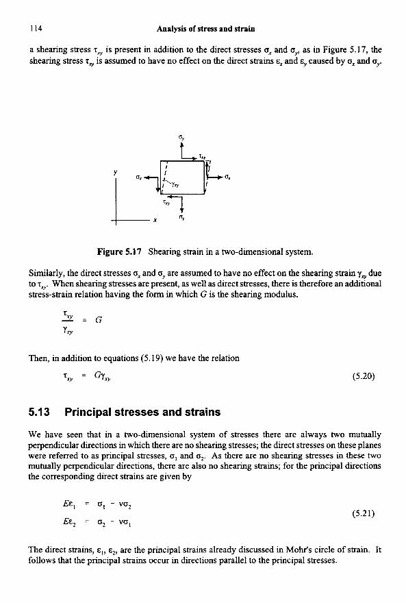
114 Analysis of stress and strain
a shearing stress T~ is present in addition to the direct stresses IS, and cry, as in Figure 5.17, the shearing stress T~ is assumed to have no effect on the direct strains E, and E~ caused by ox and oy.
Figure 5.17 Shearing strain in a two-dimensional system.
Similarly, the direct stresses IS, and isy are assumed to have no effect on the shearing strain y, due to T ~ . When shearing stresses are present, as well as direct stresses, there is therefore an additional stress-strain relation having the form in which G is the shearing modulus.
5 - G - -
y,
Then, in addition to equations (5.19) we have the relation
‘5q = e x . ” (5.20)
5.1 3 Principal stresses and strains
We have seen that in a two-dimensional system of stresses there are always two mutually perpendicular directions in which there are no shearing stresses; the direct stresses on these planes were referred to as principal stresses, IS, and IS*. As there are no shearing stresses in these two mutually perpendicular directions, there are also no shearing strains; for the principal directions the corresponding direct strains are given by
E E ~ = 0 , - vo2
E E ~ = o2 - v q (5.21)
The direct strains, E,, E,, are the principal strains already discussed in Mohr‘s circle of strain. It follows that the principal strains occur in directions parallel to the principal stresses.

Relation between E, C and Y 115
5.14 Relation between E, G and v
Consider an element of material subjected to a tensile stress ci, in one direction together with a compressive stress oo in a mutually perpendicular direction, Figure 5.18(i). The Mohr's circle for this state of stress has the form shown in Figure 5.18(ii); the circle of stress has a centre at the origin and a radius of 0,. The direct and shearing stresses on an inclined plane are given by the co- ordinates of a point on the circle; in particular we note that there is no direct stress when 28 = 90°, that is, when 8 = 45" in Figure 5.18(i).
Figure 5.18 (i) A stress system consisting of tensile and compressive stresses of equal magnitude, but acting in mutually perpendicular directions.
(ii) Mohr's circle of stress for this system.
Moreover when 8 = 45 O , the shearing stress on this plane is of magnitude o0. We conclude then that a state of equal and opposite tension and compression, as indicated in Figure 5.18(i), is equivalent, from the stress standpoint, to a condition of simple shearing in directions at 45", the shearing stresses having the same magnitudes as the direct stresses (T, (Figure 5.19). This system of stresses is called pure shear.
Figure 5.19 Pure Shear. Equality of (i) equal and opposite tensile and compressive stresses and (ii) pure shearing stress.
If the material is elastic, the strains E, and E~ caused by the direct stresses (T, are, from equations (5.1%

116 Analysis of stress and strain
1 =0
E E E,, = - (-Oo - VQ0) = -- (1 + V)
If the sides of the element are of unit length, the work done in drstorting the element is 2
1 1 0 0
2 2 ' ' E = - O o E x - d E = - ( ( l + V ) (5.22)
per unit volume of the material. In the state of pure shearing under stresses o,, the shearing strain is given by equation (5.20),
0 0 Y, = -
G
The work done in distorting an element of sides unit length is 2
1 0 0
2 2G w = - boy, = - (5.23)
per unit volume of the material. As the one state of stress is equivalent to the other, the values of work done per unit volume of the material are equal. Then
2 2 0 0 0 0 - ( l + v ) = - E 2G
and hence
E = 2G(1 + V) (5.24)
Thus v can be calculated from measured values E and G.
the form The shearing stress-strain relation is given by equation (5.20), which may now be written in
Ey, = 2(1 + v)r, (5.25)

Relation between E, G and v
For most metals v is approximately 0.3; then, approximately,
E = 2(1 + v)G = 2.6G
117
(5.26)
Problem 5.5 From tests on a magnesium alloy it is found that E is 45 GNIm’ and G is 17 GN/m*. Estimate the value of Poisson’s ratio.
Solution
From equation (5.24),
v = - - E 1 = - - 45 1 = 1.32 - 1 2G 34
Then
v = 0.32
Problem 5.6 A thm sheet of material is subjected to a tensile stress of 80 MNIm’, in a certain direction. One surface of the sheet is polished, and on this surface fme lines are ruled to form a square of side 5 cm, one diagonal of the square being parallel to the direction of the tensile stresses. If E = 200 GN/m’, and v = 0.3, estimate the alteration in the lengths of the sides of the square, and the changes in the angles at the comers of the square.
Solution
The diagonal parallel to the tensile stresses increases in length by an amount
The diagonal perpendicular to the tensile stresses diminishes in length by an amount
0.3 (28.3 x = 8.50 x m
The change in the corner angles is then
1 1 - [(28.3 + 8.50)10-6] - = 52.0 x radians = 0.0405” 0.05 fi

118 Analysis of stress and strain
The angles in the line of pull are diminished by h s amount, and the others increased by the same amount. The increase in length of each side is
1 - [(28.3 - 8.50)10-6] = 7.00 x 1O-6 m 2 4
5.1 5 Strain ‘rosettes’
To determine the stresses in a material under practical loadmg conditions, the strains are measured by means of small gauges; many types of gauges have been devised, but perhaps the most convenient is the electrical resistance strain gauge, consisting of a short length of fine wire which is glued to the surface of the material. The resistance of the wire changes by small amounts as the wire is stretched, so that as the surface of the material is strained the gauge indicates a change of resistance which is measurable on a Wheatstone bridge. The lengths of wire resistance strain gauges can be as small as 0.4 mm, and they are therefore extremely useful in measuring local strains.
Figure 5.20 Finding the principal strains in a two-dimensional system by recording three linear strains, E,, E, and E, in the vicinity of a point.
The state of strain at a point of a material is defined in the two-dimensional case if the direct strains, E, and E ~ , and the shearing strain, y9, are known. Unfortunately, the shearing strain y, is not readily measured; it is possible, however, to measure the direct strains in three different directions by means of strain gauges. Suppose E,, E, are the unknown principal strains in a two-
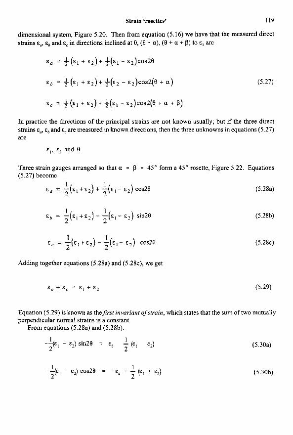
Strain 'rosettes' 119
dimensional system, Figure 5.20. Then from equation (5.16) we have that the measured direct strains E,, and E, in directions inclined at 0, (e + a), (e + a + p) to E, are
E, = + E 2 ) + - E ~ ) C O ~
& b = +-(E1 + c 2 ) + +(c2 - E ~ ) c o s ~ ( ~ + a) (5.27)
E, = +(c l + c 2 ) + +(cl - E ~ ) c o s ~ ( ~ + a + p)
In practice the directions of the principal strains are not known usually; but if the three direct strains E,, and E, are measured in known directions, then the three unknowns in equations (5.27) are
e l , e2 and 8
Three strain gauges arranged so that a = p = 45" form a 45" rosette, Figure 5.22. Equations (5.27) become
1 1 2 2
E, = - ( E ~ + E ~ ) + - (E] - E ~ ) COSB (5.28a)
(5.28b) 1 1 2 2
= - ( E ~ + E ~ ) - -(E] - E ? ) sin28
(5.28~) 1 1 2 2
E, = E ~ ) C O S ~ C I
Adding together equations (5.28a) and (5.28c), we get
E, + E, = E, + E * (5.29)
Equation (5.29) is known as thefirst invariant ofstrain, which states that the sum of two mutually perpendicular normal strains is a constant.
From equations (5.28a) and (5.28b).
1 1 - e2) sin28 = eh - (el - e 2 )
1 - EJ COSD = - E , + 1 (el + e2)
(5.3 Oa)
(5.30b)

120
Dividing equation (5.30a) by (5.30b), we obtain
Analysis of stress and strain
1 ‘h - $ 1 + ‘2)
-Ea + $1 + ‘2)
tan20 = (5.31) 1
Substituting equation (5.29) into (5.31)
(5.32) (‘a - 2Eb + ‘ c ) tan20 =
(Ea - E,)
To determine E, and c2 in terms of the known strains, namely E, E~ and E,, put equation (5.32) in the form of the mathematical triangle of Figure 5.2 1.
Figure 5.21 Mathematical triangle from equation (5.32).
2 2 2 2 2 * + 4 E h + E, - 4EaEh - 4ebE, + 2EaE, + Ea 4. Eb - 2EaEh
= fi /(‘a - ‘ b y + (&c - ‘h)2
Ea - ‘c
fi /(&a - ‘ b y + (‘E - ‘ b y
:. c o s 2 0 = (5.33)
Ea - 2 E b + E,
and sin28 = (5.34) fi /(‘a - ‘h)Z + (&c - ‘ b y

Strain 'rosettes' 121
Substituting equations (5.33) and (5.34) into equations (5.30a) and (5.30b) and solving,
fi (5.35) 1 '1 = #a + ~ c ) + 1 /(&a - & b y + (E, - ~ h y
E2 = 3, + Ec) - - fi $/(Ea - Eby + kc - EJ (5.36) 2
8 is the angle between the directions of E, and E,, and is measured clockwise from the direction of E,.
Figure 5.22 A 45" strain rosette. Figure 5.23 Alternative arrangements of 120" rosettes.
The alternative arrangements of gauges in Figure 5.23 correspond to 120" rosettes. On putting a = f3 = 120" inequations(5.27), we have
(5.37a) 1 1 2 2
1 1 2 2
1 1 2
E, = - ( E ~ + E ~ ) + - ( E ~ - E ~ ) COS^^
& b = --(cl+ c 2 ) - - ( E ~ - 2 -cos28- -sin20 (5.37b) 2
(5.37c)
E ,i: . " I E )[; v 2
E, = -(cl t c 2 ) - ?(E' - 2 -COS 28 + --sin20

122 Analysis of stress and strain
Equations (5.37b) and (5.37~) can be written in the forms
2 1 2
Adding together equations (5.37a), (5.38a) and (5.38b), we get:
3 2
EU + Eh + Ec = - (E, + E*)
or
2 3
El + E2 = - (En + Eh + E c )
Taking away equation (5.38b) from (5.38a),
Taking away equation (5.38b) from (5.37a)
Dividing equation (5.41) by (5.40)
or
(5.38a)
(5.38b)
(5.39)
(5.40)
(5.41)
(5.42)

Strain ‘rosettes’ 123
To determine E, and E* in terms of the measured strains, namely E,, E~ and E,, put equation (5.42) in the form of the mathematical triangle of Figure 5.24.
1 & I = -(Eu + & b + E‘) + -
3 3 1

124
These give
Analysis of stress and strain
E o1 = - (El + ve,)
(€2 i. V&*)
1 - 3
E o2 = - 1 - 9
(5.47)
Equations (5.18) and (5.47) are for the plane stress condition, which is a two-dimensional system of stress, as discussed in Section 5.12.
Another two-dimensional system is known as a plane strain condition, which is a two- dimensional system of strain and a three-dimensional system of stress, as in Figure 5.25, where
o vox E E E
EL = 0 = I - - - v o y _. (5.48a)
vox voz €y - - - O Y - - - -
E E E (5.48b)
VC (5.48~) ox v=y - 2
Ex = - - - E E E
Figure 5.25 Plane strain condition.
From equation (5.48a)
0, = v (ox + cy) (5.49)
Strain ‘rosettes’
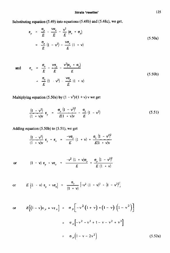
Substituting equation (5.49) into equations (5.48b) and (5.48c), we get,
= - ( l or -2)--(1 v‘Y + v ) E E
Multiplying equation (5.50a) by (1 - ?)/( 1 + v) v we get
Adding equation (5.50b) to (5.51), we get
(1 - ”) -VO Oy (1 - v’y - & + & = - 2 ( l + v ) + (1 + v)v E E(l + v)v
-2 (1 + v)oy oy (1 - 2y or (1 - v) EY + VEX = +
E E ( l + v )
or E [(1 - v) + V E ~ ] = - OY [-v’ (1 + v)’ + (1 - v’y] (1 + v)
or E [( 1 - v ) + V E , ] = o, , [ -v2(1 + v ) + ( 1 - v ) (1 - v
= o y [ - v 2 - v 3 + l - v - v 2 + v 31
= o,( l - v - 2 v 2 )
125
(5.50a)
(5.5 Ob)
(5.51)
(5.52a)

126 Analysis of stress and strain
= c r y (1+ v ) ( l - 2v)
E[(1- V) E,,+ V E X 1 :. cry =
(1 + v) (1 - 2v)
Similarly
E [ ( l - v) E, + V E y l ox =
(1 + v) (1 - 2v) (5.52b)
Obviously the values of E and v must be known before the stresses can be estimated from either equations (5.19), (5.47) or (5.52).
5.1 6 Strain energy for a two-dimensional stress system
If G, and o2 are the principal stresses in a two-dimensional stress system, the corresponding principal strains for an elastic material are, from equations (5.21),
1 = 2 (GI - vo2)
Consider a cube of material having sides of unit length, and therefore having also unit volume. The edges parallel to the direction of o, extend amounts E,, and those parallel to the direction of G, by amounts E*. The work done by the stresses o, and o, during straining is then
1 1 w = - o l & i + - o & 2 2 2 2
per unit volume of material. On substituting for E, and E, we have
This is equal to the strain energy Uper unit volume; thus
1 7 ’ u = - [o; + 0; - 2voi 02] 2E
(5.53)

Three dimensional stress systems 127
5.1 7 Three-dimensional stress systems
In any two-dimensional stress system we found there were two mutually perpendicular directions in which only direct stresses, o1 and 02, acted; these were called the principal stresses. In any three- dimensional stress system we can always find three mutually perpendicular directions in which only direct stresses, ol, o2 and o, in Figure 5.26, are acting. No shearing stresses act on the faces of a rectangular block having its edges parallel to the axes 1, 2 and 3 in Figure 5 .26 . These direct stresses are again called principal stresses.
If o1 > o2 > (r,, then the three-dimensional stress system can be represented in the form of Mohr's circles, as shown in Figure 5.27. Circle a passes through the points o1 and o2 on the o-axis, and defines all states of stress on planes parallel to the axis 3 , Figure 5.26, but inclined to axis 1 and axis 2 , respectively.
Figure 5.26 Principal stresses in a three-dimensional system.
Figure 5.27 Mohr's circle of stress for a three- Figure 5.28 Two-dimensional stress dimensional system; circle a is the Mohr's circle of the system as a particular case of a three- two-dimensional system ol, 0,; b corresponds to o,, o3 dimensional system with one of the and c to o,, ol. The resultant direct and tangential stress three principal stresses equal to zero. on any plane through the point must correspond to a point P lying on or between the three circles.

128 Analysis of stress and strain
Circle c, having a diameter (a, - aJ, embraces the two smaller circles. For a plane inclined to all three axes the stresses are defined by a point such as P within the shaded area in Figure 5.27. The maximum shearing stress is
and occurs on a plane parallel to the axis 2. From our discussion of three-dimensional stress systems we note that when one of the
principal stresses, a3 say, is zero, Figure 5.28, we have a two-dimensional system of stresses cr,, a2; the maximum shearing stresses in the planes 1-2,2-3,3-1 are, respectively,
Suppose, initially, that cr, and a2 are both tensile and that a, > a,; then the greatest of the three maximum shearing stresses is ?4 a, which occurs in the 2-3 plane. If, on the other hand, a, is tensile and a2 is compressive, the greatest of the maximum shearing stresses is % (ar - 0,) and occurs in the 1-2 plane.
We conclude from this that the presence of a zero stress in a direction perpendicular to a two- dimensional stress system may have an important effect on the maximum shearing stresses in the material and cannot be disregarded therefore. The direct strains corresponding to ci,, a, and a3 for an elastic material are found by taking account of the Poisson ratio effects in the three directions; the principal strains in the directions 1 , 2 and 3 are, respectively,
1 E
E2 = - (a2 - vag - V a l )
1 E
E3 = - (a3 - V a l - VOz)
The strain energy stored per unit volume of the material is
1 1 1 u = - a l & l + - a & + - a 3 3 & 2 2 2 z 2
In terms of a,, a2 and a3, this becomes

Volumetric strain in a material under hydrostatic pressure 129
5.18 Volumetric strain in a material under hydrostatic pressure
A material under the action of equal compressive stresses (s in three mutually perpenlcular directions, Figure 5.29, is subjected to a hydrostatic pressure, 0. The term hydrostatic is used because the material is subjected to the same stresses as would occur if it were immersed in a fluid at a considerable depth.
Figure 5.29 Region of a material under a hydrostatic pressure.
If the initial volume of the material is V,, and if h s diminishes an amount 6 Vdue to the hydrostatic pressure, the volumetric strain is
6V - vo
The ratio of the hydrostatic pressure, 0, to the volumetric strain, 6Y,’Vo, is called the bulk modulus of the material, and is denoted by K. Then
(s K = - (5 .55) [:)
If the material remains elastic under hydrostatic pressure, the strain in each of the three mutually perpendicular directions is
0 v0 v(s E = - - + + - + - E E E
(s = -- (1 - 2v)
E

130
because there are two Poisson ratio effects on the strain in any of the three directions. If we consider a cube of material having sides of unit length in the unstrained condition, the volume of the strained cube is
Analysis of stress and strain
(1 - E)3
Now E is small, so that this may be written approximately
1 - 3 E
The change in volume of a unit volume is then
3 E
which is therefore the volumetric strain. Then equation (5.55) gives the relationship
0 - 0 - E K = - - - - - 3 ~ 3(1 - 2 ~ )
We should expect the volume of a material to diminish under a hydrostatic pressure. In general, if K is always positive, we must have
1 - 2 v > o
or
1 v < - 2
Then Poisson's ratio is always less than %. For plastic strains of a metallic material there is a negligible change of volume, the Poisson's ratio is equal to %, approximately.
5.19 Strain energy of distortion
In the three-dimensional stress system of Figure 5.22 we may consider the principal stress 0, to be the resultant of stresses
and stresses
1 3 - (20, - 0 2 - 0 3 )

Strain energy of distortion
since
1 1 3 3 - (GI + Is2 + 03) + - (20, - G2 - 03) = 0,
131
Similarly, we write
1 1 3
o2 = - (0, + 0* + 03) + (202 - (r3 - 0))
1 1 3
0 3 = - (0, + o2 + 03) + 7 (203 - 0, - 02)
Now, the component '13 (oI + o2 + u2) which occurs in cl, o2 and 03, represents a hydrostatic tensile stress; the strains associated with this stress give rise to no distortion, i.e., a cube of material under stress Y3 (oI + o2 + 03) in three mutually perpendicular directions is strained into a cube. The remaining components of oI, o2 and 03, are
The strain energy associated with these stresses, which are the only stresses giving rise to distortion, is called the strain energy of distortion. The strains due to these distorting stresses are
1 1 3E 6G E ,
= - (1 + v) (20, - 0* - 03) = - [(o, - 02) + (0, - G3)]
1 1 3E 6G E 2 = - (1 + v) (20, - G3 - 0,) = - [(02 - 03) + (c2 - GI)]
1 1 3E 6G E 3
= - (1 + v) (203 - 0, - G 2 ) = - [(03 - 0]) + (a3 - 02)]
The strain energy of distortion is therefore
1 36G
U[) = - [pol - o2 - G3)2 + (202 - (T3 - 0,y + (2D3 - 0, - 02r]
per unit volume. Then
(5 .56)

132
For a two-dimensional stress system, 0, (say) = 0, and U, reduces to
Analysis of stress and strain
1 UD = 12G [(GI - 0*)2 + 0: + 43
We shall see later that the strain energy of distortion plays an important part in the yielding of ductile materials under combined stresses.
5.20 Isotropic, orthotropic and anisotropic
A material is said to be isotropic when its material properties are the same in all directions. An orthotropic material is said to exhlbit symmetric material properties about three mutually perpendicular planes. In two dimensions, typical orthotropic materials are in the form of many composites. An anisotropic material is a material that ef ibi ts different material properties in all directions.
5.21 Fibre composites
Fibre composites are very important for structures which require a large strength:weight ratio, especially when the weight of the structure is at a premium. They are likely to become even more important in the 2 1 st century and will probably revolutionise the design and construction of aircraft, rockets, submarines and warships.
To represent the elasticity of a composite, tensile modulus is used in preference to Young’s modulus of elasticity. Additionally, as most composites are usually assumed to be of orthotropic form, their material properties in one direction, (say) ‘x’ are likely to be different to a direction perpendicular to the ‘x’ direction, (say) ‘y’. Composites usually consist of several layers of fibre matting, set in a resin, as shown by Figure 5.30. To gain maximum strength the layers of fibre matting are laid in different directions. In this Chapter, the term lamina or ply will be used to describe a single layer of the composite structure and the term laminate or composite will be used to define the entire mixture of plies and resin.
If the material properties of the fibre composite are orthogonal, the following relationship applies:
V, Ey = V, E, (5.57)
Figure 5.30 Five layers of fibre reinforcement.
Fibre composites 133
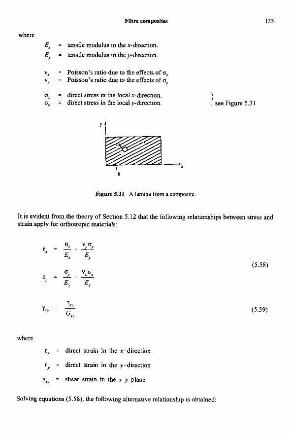
where E, = tensile modulus in the x-direction. E,, = tensile modulus in the y-direction.
vx = Poisson's ratio due to the effects of ox vv = Poisson's ratio due to the effects of cy
ox = duect stress in the local x-direction. oy = direct stress in the localy-direction. 1 see Figure 5.3 1
Figure 5.31 A lamina from a composite.
It is evident from the theory of Section 5.12 that the following relationshps between stress and strain apply for orthotropic materials:
ox vyo,, e x = - - -
Ex Ey
= y - vx',
E y E x
( 5 . 5 8 ) o
&Y
(5 .59) - 5 Y, - -
GXV
where
ex = direct strain in the x-direction
E" = direct strain in the y-direction
y, = shear strain in the x-y plane
Solving equations (5.58), the following alternative relationship is obtained:

134 Analysis of stress and strain
In matrix form, equations (5.58) and (5.59) can be written as
where [s] is the compliance matrix.
From equations (5.59) and (5.60)
(5.60)
(5.61)
(5.62)
(5.63)
where

Fibre composites 135
Q66 = Gx.v = shear modulus
(5.64)
[Q] = thestifiessmatrix
= the inverse of [SI
The problem with the above relationships are that they are all in the local co-ordinate system of the lamina, namely x and y. However, as each layer of fibres may have a different direction for its local co-ordinate system, it will be necessary to refer all relationships to a fixed global system, namely, X and Y, as shown by Figure 5.3 1.
Now from equations (5.4) and (5.5)
2 o x = o x cos2 e + o y sin e + 2r, sine case o y = o x + 90° = o x sin2 8 + a y cos 8 - 2 r m sin0 cos0
T~ = - o x sin6 cos6 + m y sine cos6 + r X Y
(5 .65) 2
where ox, oy and 'I, are local stresses and ox, o, and r, are global or reference stresses; in matrix form equations (5.65) appear as:
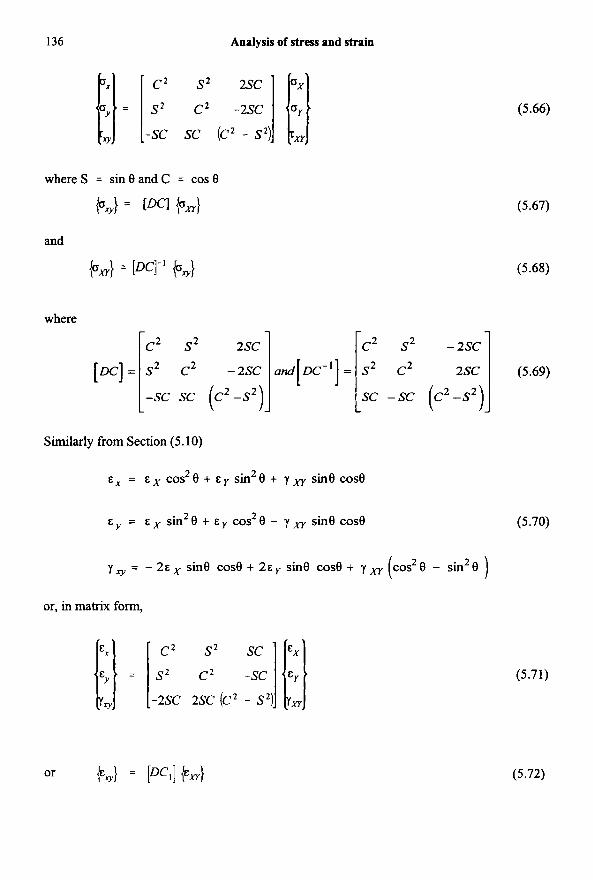
136 Analysis of stress and strain
= Ei c’ s2 2sc s’ c’ -2sc : -sc sc (c’ - s
(5.66)
(5.67)
(5.68)
where
c2 s2 2sc c2 s2 - 2sc
-sc sc (c2-s2)
Similarly from Section (5.10)
E, = E X cos 8 + E y sin e + yxr sine wse 2 2
E~ = E~ sin2e + c y ms2e - y x r sine case (5.70)
1 yxy = - 2 E x sine COS^ + 2cy sine case + yxr ws2e - sin2e ( or, in matrix form,
- -
c2 s’ sc s’ c’ -sc -2sc 2sc (c’ - s’
(5.71)
(5.72)

Fibre composites
Now from equation (5.63),
(4 = rQl{Ew]
(4 = [QI [ m I ] { E X Y I
(4 = [4{4
but from equation (5.72),
but from equation (5.67),
... [DC] (0 X Y ) = [Q] [DCI] {EH)
or
( ~ H ) = [XI-' [e] [ W ] ( ~ r n )
or
( O H ] = [Q']{EH)
where
[Q'] =
1 1 1 711 412 416
1 I 1 721 q22 q 2 6
1 1 1 761 q62 966
137
(5.73)
(5.74)
qll I 1 = - [E, cos4 e + E~ sin4 e + (2v, E,, + 4 y ~ ) cos2~sin28]
Y
1 I 1 Y
qI2 = qZ1 = - [v, E,, ( C O S ~ B + sin4e) + (E, + E" - 4yG) cos2e sin20]

138 Analysis of stress and strain
I 1
Y 916 I - - q61 = - [cos3e sine (Ex - v$,, - 2yG) - cos8 sin3@ (E,, - v$,,, - 2yG)]
q22 I 1 = - [Ev cos4 8 + E, sin4 e + sin2B cos2 e (2v& + 4yG)]
Y .
q26 1 - - q62 I 1 = - [COS e sin3 8 (Ex - vg,, - 2yG) - cos3 8 sin 8 (Ev - v, E,, - 2yG)]
Y
1 1 . = - [sm2e cos2 e ( E ~ + E, - 2vx E, - 2yG) + y~ (cos4 e + sin4 e)] 966
Y
where
y = (1 - vr v,)
Similarly, to obtain the global strains of the lamina or ply of Figure 5.32 in terms of the global stresses, consider equation (5.61), as follows.
Now
(Em) = ['J +rv}
so that from equation (5.67)
(Ex,} = [SI WI (oxy}
and from equation (5.72)
(5.75)
where

I 11 ';2 ','6
[''I = 1:; Si, si,- 'l2 si,a
(i) Section through the laminate (ii) strain distribution (iii) stress distribution
Figure 5.33 In-plane stresses and strains in a laminate.
= [Del]' 1'1 [''I
140 Analysis of stress and strain
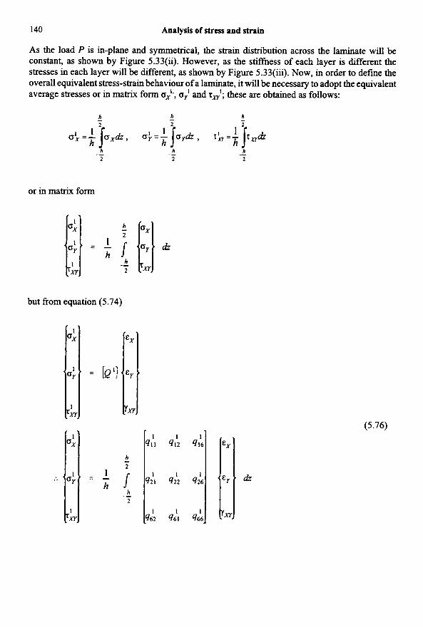
As the load P is in-plane and symmetrical, the strain distribution across the laminate will be constant, as shown by Figure 5.33(ii). However, as the stiffness of each layer is different the stresses in each layer will be different, as shown by Figure 5.33(iii). Now, in order to define the overall equivalent stress-strain behaviour of a laminate, it will be necessary to adopt the equivalent average stresses or in matrix form o,',, o; and T ~ ' ; these are obtained as follows:
h h h 2 2 2
-_ -- -_
or in matrix form
but from equation (5.74)
(5.76)
In-plane equations for a symmetric laminate or composite 141
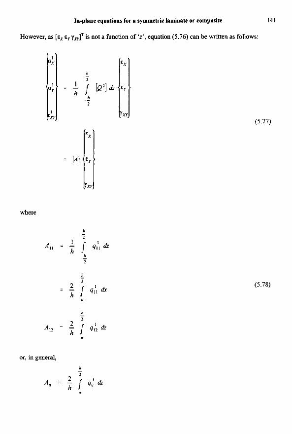
However, as [ E ~ E, yH]' is not a function of 'z', equation (5.76) can be written as follows:
where
h 2
--
h -
or, in general,
(5.77)
(5.78)

142 Analysis of stress and strain
For the kth lamina of the laminate, the q1 terms are constant, hence the integrals for the A terms can be replaced by summations:
(5.79)
and similarly for the other values of A,,
where
h,
q,,(k) = kth value of qi I
v,
= thickness of the kth lamina or ply
= (2hJh) = the volume fraction in the kth lamina
Once the srzfiness matrix [ A ] is obtained, it can be inverted to obtain the compliance matrix [a] and hence, the equivalent material for the laminate properties are as follows:
E , = - , 1 E , = - - , 1 G x y = - 1 , v x = - -a12 and vY = - -a12 a, I a22 a66 a , 1 a22
Experience has shown that the diagonal terms in the laminate's stiffness matrix are considerably larger than the off-diagonal terms, so that E, etc. can be approximated by
E, c v k EX(kC) Cos40k
where k refers to the kth lamina of the laminate.
5.23 Equivalent elastic constants for problems involving bending and twisting
For problems in this category, the equivalent stress resultants for the laminate are o i , o;, Tmi, M i , M; and Mml, where the former three symbols are in-plane and the latter three are out-of-plane bending and twisting terms.
Equivalent elastic constants for problems involving bending and twisting 143
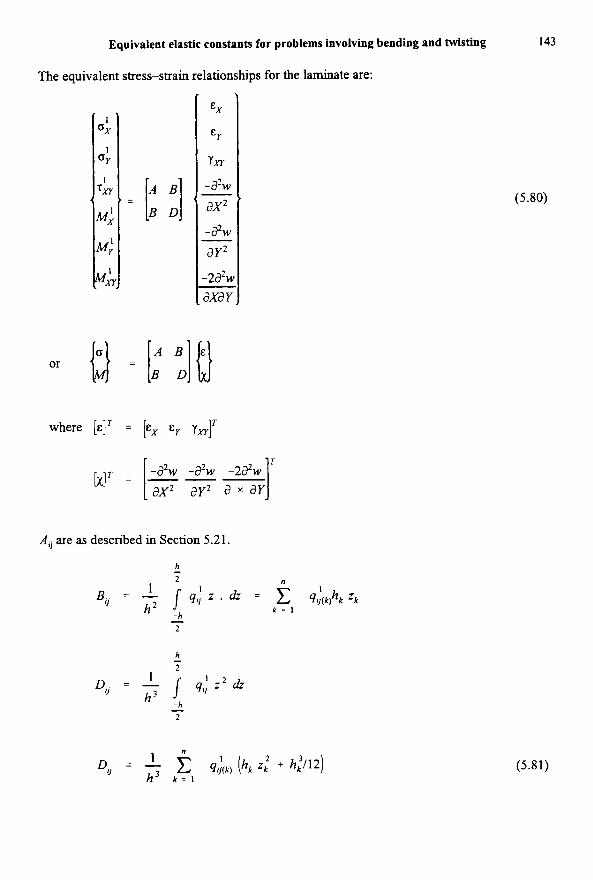
The equivalent stress-strain relationships for the laminate are:
or [ =
A B D B1 ax2 - 2 W
ay2
-2a2w axay
B D A "It1 where [E]' = [E, yX]'
r -gW -aZw -2a2w
A , are as described in Section 5.21.
h -
h 2 -
1 D, = - 1 ql; z 2 dz h 3 -h -
2
1 1 D , , = - ? h 3 k = i q r / ( k ) (hk 'k' +
(5.80)
(5.81)

144 Analysis of stress and strain
where
w = out-of-plane deflection
n
k = thekthplyorlamina
z,
= number of laminates or plies
= distance of the centre plane of the kth ply
For symmetrical laminates, B, = 0, however, for design purposes, the following relationship is often used:
where
[u] = [A]-' (see Section 5.21)
Another way of looking at the components of [D] are as follows:
(5.82)
where k = thekthply
I, = the second moment of area of the kth ply or lamina about the neutral axis of the laminate or composite
the second moment of area of the entire laminate or composite about the neutral axis
1- =
5.24 Yielding of ductile materials under com bined stresses
It was noted in Section 5.3 that when a polished bar of mild steel is loaded in tension, strain figures are observable on the surface of the bar after the yield point has been exceeded. The figures take the form of 'lines' inclined at about 45" to the axis of the bar; tfus direction corresponds to the planes of maximum shearing stress in the bar; the 'lines' are, in fact, bands of metal crystals

Yielding of ductile materials under combined stresses 145
shearing over similar bands. That yieldmg takes place in this way suggests that the crystal structure of the metal is relatively weak in shear; yielding takes the form of sliding of one crystal plane over another, and not the tearing apart of two crystal planes.
This form of behaviour-yielding by a shearing action-is typical of ductile materials. We note firstly that ifa material is subjected to a hydrostatic pressure (I, the three principal stresses (I,, cr2 and (I, in a three-dimensional system are each equal to (I. A state of stress of h s sort exists in a solid sphere of material subjected to an external pressure (I, Figure 5.34. As the three principal stresses are equal in magnitude, there are no shearing stresses in the material; if yielding is governed by the presence of shearing on some planes in a material, then no yielding is theoretically possible when the material is under hydrostatic pressure.
Figure 5.34 A solid sphere of material under hydrostatic pressure.
For a two-dimensional stress system one of the three principal stresses of a three-dimensional system is zero. We consider now the yielding of a mild steel under different combinations of the principal stresses, (I, and 02, of a two-dimensional system; in discussing the problem we keep in mind the presence of a zero stress perpendicular to the plane of (I, and 02, Figure 5.27.
Figure 5.35 Yield envelope of a two Figure 5.36 In a two-dimensional stress system, one of the three principal stresses -
(aj say) is zero. dimensional stress system when the material yields according to the maximum shearing
stress criterion.

146 Analysis of stress and strain
Suppose we conduct a simple tension test on the material; we may put o2 = 0, and yielding occurs when o, = cry, (say)
This yielding condition corresponds to the point A in Figure 5.35. If the material has similar properties in tension and compression, yielding under a compressive stress o, occurs when o, = -cry; this condition corresponds to the point C in Figure 5.35. We could, however, perform the tension and compression tests in the direction of oz, Figure 5.35; if the material is isotropic -that is, it has the same properties in all directions-yielding occurs at the yield stress oy; we can thus derive points B and D in the yield diagram, Figure 5.35.
We consider now yielding of the material when both Q, and 02, Figure 5.36, are present; we shall assume that yielding of the mild steel occurs when the maximum shearing stress attains a critical value; from the simple tensile test, the maximum shearing stress at yielding is
1 %l, = y or
which we shall take as the critical value. Suppose that o, > 02, and that both principal stresses are tensile; the maximum shearing stress is
1 1 2
T,, = - (ol - 0) = 2 o1
and occurs in the 3-1 plane of Figure 5.36; T- attains the critical value when
1 - 1 T o1 - - or, or o1 = or 2
Thus, yielding for these stress conditions is unaffected by oz. In Figure 5.35, these stress conditions are given by the line AH. If we consider similarly the case when o1 and o2 are both tensile, but o2 > (I,, yielding occurs when o2 = ay, giving the line BH in Figure 5.35.
Figure 5.37 Plane of yielding when both Figure 5.38 Plane of yielding when the principal stresses tensile and (J, > 02. principal stresses are of opposite sign.
By making the stresses both compressive, we can derive in a similar fashion the lines CF and DF of Figure 5.36.

Yielding of ductile materials under combined stresses I47
But when 6, is tensile and o2 is compressive, Figure 5.36, the maximum shearing stress occurs in the 1-2 plane, and has the value
Yielding occurs when
1 (ol - 02) = - 1 cy, or o1 - o2 = oy
2
This corresponds to the line AD of Figure 5.36. Similarly, when o, is compressive and o2 is tensile, yielding occurs when corresponding to the line BC of Figure 5.36.
The hexagon AHBCFD of Figure 5.36 is called a yield locus, because it defines all combinations of 6, and o2 giving yieldmg of mild steel; for any state of stress within the hexagon the material remains elastic; for this reason the hexagon is also sometimes called a yield envelope. The criterion ofyielding used in the derivation of the hexagon of Figure 5.36 was that of maximum shearing stress; the use of h s criterion was first suggested by Tresca in 1878.
Not all ductile metals obey the maximum shearing stress criterion; the yielding of some metals, including certain steels and alloys of aluminium, is governed by a critical value of the strain energy of distortion. For a two-dimensional stress system the strain energy of distortion per unit of volume of the material is given by equation (5.83). In the simple tension test for which o2 = 0, say, yielding occurs when 6, = oy. The critical value of U, is therefore
2 1 1 GY
6G 6G 6G u, = - [o: - G I o2 + o;] = - [o; - cy (0) + 021 = -
Then for other combinations of o1 and 02, yielding occurs when
(5.83) 2 2 2 o1 - GI o2 + o2 = oy
The yield locus given by this equation is an ellipse with major and minor axes inclined at 45 O to the directions of oI and 02, Figure 5.39. This locus was first suggested by von Mises in 1913.
For a three-dimensional system the yield locus corresponding to the strain energy of distortion is of the form
(ol - 02)' + (02 - 03)2 + (03 - o,r = constant
l k s relation defines the surface of a cylinder of circular cross-section, with its central axis on the line 0, = o2 = 0,; the axis of the cylinder passes through the origin of the o,, 02, u, co-ordinate

148 Analysis of stress and strain
system, and is inclined at equal angles to the axes (I~, o2 and (I~, Figure 5.40. When (I, is zero, critical values of 6, and cr2 lie on an ellipse in the cs,-02 plane, corresponding to the ellipse of Fimre 5.39.
Figure 5.39 The von Mises yield locus for a Figure 5.40 The von Mises yield locus for a two-dimensional system of stresses. three-dimensional stress system.
I
Figure 5.41 The maximum shearing stress (or Tresca) yield locus for a three-dimensional stress system.
When a material obeys the maximum shearing stress criterion, the three-dimensional yield locus is a regular hexagonal cylinder with its central axis on the line (I, = c2 = o3 = 0, Figure 5.40. When o3 is zero, the locus is an irregular hexagon, of the form already discussed in Figure 5.36.
The surfaces of the yield loci in Figures 5.40 and 5.41 extend indefinitely parallel to the line crI = (I* = 03, which we call the hydrostatic stress line. Hydrostatic stress itself cannot cause yielding, and no yielding occurs at other stresses provided these fall within the cylinders of Figures 5.40 and 5.41.

Elastic breakdown and failure of brittle material 149
The problem with the maximum principal stress and maximum principal strain theories is that they break down in the hydrostatic stress case; this is because under hydrostatic stress, failure does not occur as there is no shear stress. It must be pointed out that under uniaxial tensile stress, all the major theories give the same predictions for elastic failure, hence, all apply in the uniaxial case. However, in the case of a ductile specimen under pure torsion, the maximum shear stress theory predicts that yield occurs when the maximum shear reaches 0.5 cry, but in practice, yield occurs when the maximum shear stress reaches 0.577 of the yield stress. This last condition is only satisfied by the von Mises or &stortion energy theory and for this reason, this theory is currently very much in favour for ductile materials.
Another interpretation of the von Mises or distortion energy theory is that yield occurs when the von Mises stress, namely om, reaches yield.
In three dimensions, o,, is calculated as follows:
CYUrn = Ac1 - 02), +(ol - “ 3 ) 2 + ( O Z - “:)]/J;
In two-dimensions, o3 = 0, therefore equation (5.84) becomes:
(5.84)
2 “urn = /(“? + “ 2 - “ 1 “ 2 ) (5.85)
5.25 Elastic breakdown and failure of brittle material
Unlike ductile materials the failure of brittle materials occurs at relatively low strains, and there is little, or no, permanent yielding on the planes of maximum shearing stress.
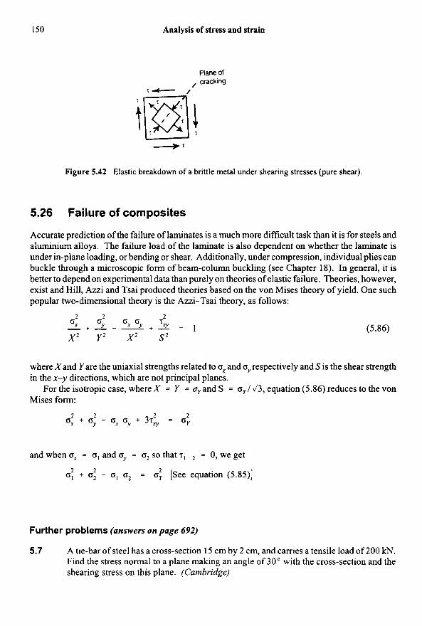
Some brittle materials, such as cast iron and concrete, contain large numbers of holes and microscopic cracks in their structures. These are believed to give rise to high stress concentrations, thereby causing local failure of the material. These stress concentrations are llkely to have a greater effect in reducing tensile strength than compressive strength; a general characteristic of brittle materials is that they are relatively weak in tension. For this reason elastic breakdown and failure in a brittle material are governed largely by the maximum principal tensile stress; as an example of the application of this criterion consider a concrete: in simple tension the breaking stress is about 1.5 MN/m2, whereas in compression it is found to be about 30 MN/m2, or 20 times as great; in pure shear the breaking stress would be of the order of 1.5 MN/m2, because the principal stresses are of the same magnitude, and one of these stresses is tensile, Figure 5.42. Cracking in the concrete would occur on planes inclined at 45” to the directions of the applied shearing stresses.
150 Analysis of stress and strain
Figure 5.42 Elastic breakdown of a brittle metal under shearing stresses (pure shear).
5.26 Failure of composites
Accurate prediction of the failure of laminates is a much more difficult task than it is for steels and aluminium alloys. The failure load of the laminate is also dependent on whether the laminate is under in-plane loading, or bending or shear. Additionally, under compression, individual plies can buckle through a microscopic form of beam-column buckling (see Chapter 18). In general, it is better to depend on experimental data than purely on theories of elastic failure. Theories, however, exist and Hill, Ami and Tsai produced theories based on the von Mises theory of yield. One such popular two-dimensional theory is the Azzi-Tsai theory, as follows:
2 2 2
(5.86) ox cy - + - = ox ay Txy , - + - - x 2 Y Z x2 s2
where Xand Yare the uniaxial strengths related to ox and o,, respectively and S is the shear strength in the x-y directions, whch are not principal planes.
For the isotropic case, where X = Y = or and S = or/ J3, equation (5.86) reduces to the von Mises form:
2 2 2 2 0, + oy - 0, 0." + 3Tv = or
andwheno, = o, ando, = o , so tha t~ , . , = 0,weget 2 2 2 o, + oz - o, o2 = or [See equation (5 .85 ) ]
Further problems (answers on page 692)
5.7 A tie-bar of steel has a cross-section 15 cm by 2 cm, and carries a tensile load of 200 kN. Find the stress normal to a plane making an angle of 30" with the cross-section and the shearing stress on this plane. (Cambridge)

Further problems 151
5.8 A rivet is under the action of shearing stress of 60 MN/mz and a tensile stress, due to contraction, of 45 MN/m2. Determine the magnitude and direction of the greatest tensile and shearing stresses in the rivet. (RNEC)
5.9 A propeller shaft is subjected to an end thrust producing a stress of 90 MN/m2, and the maximum shearing stress arising from torsion is 60 MN/m2. Calculate the magnitudes of the principal stresses. (Cambridge)
At a point in a vertical cross-section of a beam there is a resultant stress of 75 MN/m2, whch is inclined upwards at 35 " to the horizontal. On the horizontal plane through the point there is only shearing stress. Find in magnitude and direction, the resultant stress on the plane which is inclined at 40 " to the vertical and 95 " to the resultant stress. (Cambridge)
5.1 0
5.11 A plate is subjected to two mutually perpendicular stresses, one compressive of 45 MN/m2, the other tensile of 75 MN/m2, and a shearing stress, parallel to these directions, of 45 MN/m2. Find the principal stresses and strains, taking Poisson's ratio as 0.3 and E = 200 GN/m2. (Cambridge)
5.1 2 At a point in a material the three principal stresses acting in directions Ox, O,,, O,, have the values 75, 0 and -45 MN/m2, respectively. Determine the normal and shearing stresses for a plane perpendicular to the xz-plane inclined at 30" to the xy-plane. (Cam bridge)