4/RT/12 Firm Credit in Europe: A Tale of Three Crises

4/RT/12

Firm Credit in Europe:

A Tale of Three Crises

Sarah Holton, Martina Lawless and Fergal McCann

1

Firm credit in Europe: A tale of three crises

Sarah Holton, Martina Lawless and Fergal McCann∗

Central Bank of Ireland

June 29, 2012

Abstract

This paper analyses the effects of the recent euro area economic, financial and debt crisis on SMEs’

access to bank finance. We use a survey on access to finance of SMEs in the euro area carried out by

the European Central Bank during 2009 and 2010 to examine the impact of macroeconomic factors

on developments in loan applications and approvals as well as changes in credit terms and conditions.

At the country level, we identify three distinct aspects of the recent crisis in Europe affecting firm

credit through different channels. A weak real economy is found to affect the demand for bank financ-

ing. Financial conditions (proxied by the median credit default swap for banks in each country and

sovereign yields) predominantly affect the probability of loan rejection and the terms and conditions

of credit rather than the demand for credit. We interpret this as evidence of a bank balance sheet

channel negatively impacting credit provision. Crucially, the level of debt overhang affects all aspects

of SME financing, with suggestive evidence that the effect on credit rejection operates through the

bank balance sheet channel, as opposed to being due to the borrower balance sheet.

∗We thank Patrick Honohan, Kieran McQuinn and participants of the Central Bank of Ireland’s con-

ference on the Irish SME Lending Market for helpful comments. The views expressed in this paper are

our own, and do not necessarily reflect the views of the Central Bank of Ireland or the ESCB. E-mail:

[email protected], [email protected] or [email protected].

Non Technical Summary

This paper analyses the effects of the recent euro area economic, financial and debt crisis on SMEs’

access to bank finance. We use a survey on access to finance of SMEs in the euro area (SAFE) carried

out by the European Central Bank (ECB) during 2009 and 2010, which allows us to separate banks’

supply of loans from firms’ demand for credit. It also provides a distinction between firms’ perception

of the availability of finance and their actual experience obtaining credit and the terms and conditions

at which they receive it. We can then test what micro level firm characteristics and macroeconomic

factors affect each of these different components of credit access.

We consider a range of real, financial and debt stock variables that can influence access to finance

and discuss their possible impact on supply, demand, and credit conditions. We delineate the European

crisis into three distinct components: the real economy, the sovereign/financial sector, and private

sector debt overhang. We use GDP growth to capture real economic effects, and use sovereign bond

yields and banks’ credit default swaps (CDS) to capture the impact of financial variables on credit

conditions and loan supply. We also include total private sector indebtedness and sector level debt

measures to capture debt overhang. These two distinct measures represent different aspects relating

to banks’ and firms’ balance sheets.

Overall, we find that larger and older firms face the lowest risk of having loan applications rejected,

but that age and size are less important for firms’ perceptions of credit availability than they were for

actual experience of obtaining a loan. Two key variables in explaining perceptions of a reduction in

credit availability were if the firm reported a deterioration in profits or negative prospects.

The real economy is shown to affect demand for credit, but not the supply or conditions. We also

find that sovereign yields and bank CDS levels affect both the quantity supplied as well as the terms

and conditions such finance. Of the macroeconomic variables, most significantly we find that the level

of private sector indebtedness affects all aspects of SME financing: credit supply (captured by loan

rejections and terms and conditions) and demand.

The importance of the measure of debt overhang points to the hugely damaging and long-lasting

effect of credit booms which has been identified previously by authors such as Reinhart and Rogoff

(2009). From a policy perspective, one can conclude that the sovereign and financial crisis is spilling

over into the real economy through tougher credit supply conditions being imposed on potential borrow-

ers. In this way it is likely to be causing a credit crunch unexplained by borrower-level characteristics.

However, the chief culprit in the decline of credit, from a supply and demand perspective, has been

the credit bubble of the last decade which created a large and debilitating debt overhang in many euro

area economies. This over-indebtedness is affecting borrowers’ demand for financing and is affecting

supply decisions through a bank balance sheet channel and terms and conditions of financing through

a borrower balance sheet channel. The findings point to a worrying and potentially long-lasting impact

of the credit boom on countries with highly indebted private sectors.

1 Introduction

Europe has been experiencing serious economic turmoil in recent years putting financial markets and

sovereign debt markets under almost unprecendented pressure. This paper looks at how these events

have affected firms’ financing across the euro area by examining loan applications, rejection rates and

changes in the terms and conditions of lending. Our paper exploits cross-country micro-level data on

European Small and Medium Enterprises (SMEs) to identify country-level characteristics that have

driven changes in credit supply and demand. We identify three separate but connected aspects of

the European crisis that have affected lending: a real economic crisis (measured by real GDP), a

financial/sovereign crisis (sovereign bond yields, banks’ CDS) and a private sector debt overhang crisis

(private credit to GDP and sector debt to output).

Past studies have emphasised the importance of separating supply and demand drivers of credit

growth (Adrian and Shin, 2009) and analysed the extent to which credit provision is affected by bank

and firm balance-sheet strength. Changes in credit supply related to banks’ balance sheets are classified

as the bank lending or pure supply side channel and those related to firms’ balance sheets are often

referred to simply as the balance sheet channel (Bernanke and Gertler, 1995). Recent literature using

loan application data identifies evidence of this bank lending channel that operates independently of

firms’ balance sheet quality (Jimenez, Ongena, Peydro, and Saurina (Forthcoming)), and that this

becomes more active during times of crisis (Jimenez, Ongena, Peydro, and Saurina, 2012).

As comparable micro data across countries is rarely available, it has been difficult to examine the

relative impact of macroeconomic factors and the channels through which they operate on the supply

and demand for credit. The survey data we use allow us to separate supply and demand, while the

cross-country nature of our data allows us to identify specific country and time-varying drivers of crisis-

era shifts in credit supply and demand, thus filling this gap. We focus on bank credit as it has been

shown to be the chief form of financing available to SMEs (Beck, Demirguc-Kunt, and Maksimovic,

2008).

One striking finding relates to the notable impact of debt overhang on all aspects of SME financing

(the supply side measures of loan rejection and credit terms and condition, and also demand for loans).

This suggests that countries with the largest accumulated pre-crisis debt levels will face more credit

rationing and tightened supply-side conditions.1 A high ratio of private credit to GDP can lead to

bank and borrower-level deleveraging requirements through the bank lending and borrower balance

sheet channels respectively (both Ciccarelli, Maddaloni, and Peydro (2010) and Jimenez, Ongena,

1Similar to Stiglitz and Weiss (1981) we mean credit rationing as the excess demand for loanable funds

which is not satisfied as “banks deny loans to borrowers who are observationally indistinguishable from those

who receive loans.”

1

Peydro, and Saurina (Forthcoming) distinguish between these channels). Our evidence suggests that

the effect of debt overhang on credit mainly comes through the banks’ balance sheets (pure supply

channel) rather than the borrowers’ balance sheet, as it is total bank credit to the private sector that

has a statistically significant effect on supply, and not the levels of debt in the specific sectors.

Beyond our findings on debt overhang, we also find distinct effects of the real and sovereign/financial

crises. A weaker real economy is primarily associated with lower credit demand. Financial and

sovereign factors mostly lead to tighter supply conditions, both through credit rationing and higher

interest rates and lower available loan amounts. This provides evidence of a micro-level lending channel

through which sovereign and financial problems can cause heterogeneity in monetary policy transmis-

sion in the euro area and can exacerbate recessions by constraining credit provision to the real economy.

The concern that “transmission is threatened” in countries where “sovereign debt and bank funding

markets have virtually seized up” (Bini Smaghi, 2011) appears to be validated by our findings.

Our identification of supply side drivers of adverse credit conditions which are not explained by

borrower-level characteristics has implications outlined in a large literature on the impact of such

problems on the real economy. Campello, Graham, and Harvey (2010) show that firms that are

financially constrained planned lower employment and technology, capital and marketing expenditure

than matched unconstrained firms, while Mach and Wolken (2011) show that credit constraints are of

vital importance in predicting which small firms exit the market.

The paper is organised as follows: Section 2 discusses the literature and section 3 describes the

data used. Section 4 reports results on the firm and country characteristics affecting different elements

of credit access and section 5 concludes.

2 Literature, Theory and Testable Hypotheses

In this section, we briefly review some of the literature on the credit channel of monetary policy and

the theories relevant to the supply and demand of credit to provide a framework for understanding

which macroeconomic explanatory variables may affect either supply of credit, demand for credit, or

both, before we test our hypotheses in Section 4.

2.1 Credit Channel literature and disentangling credit supply and demand

The credit channel literature deals with “imperfect information and other “frictions” in credit markets”

and is concerned with the effectiveness of the monetary policy transmission mechanism in providing

finance to the real economy (Bernanke and Gertler (1995)). The credit channel includes two other

channels already mentioned, namely the bank lending channel and the balance sheet channel which

2

deal with the impact of banks’ and borrowers’ balance sheets respectively on the supply of credit.

Peek and Rosengren (1995) provide an overview of the bank lending channel and highlight the effect

of banking structures on lending to firms.

One of the challenges faced by this literature relates to problems in delineating between supply and

demand effects in analysing movements in credit (Kashyap and Stein, 2000). Certain contributions have

focused on distinguishing between these supply and demand effects, using firm level data (Kashyap,

Stein, and Wilcox, 1993), firm and bank data together (Albertazzi and Marchetti, 2010) and bank

lending survey data (Hempell and Kok Sorensen (2010), Ciccarelli, Maddaloni, and Peydro (2010)

and Del Giovane, Eramo, and Nobili (2010)). Using loan application data for Spain, which includes

information on both firm and bank balance sheets, Jimenez, Ongena, Peydro, and Saurina (2012) find

evidence that the bank lending channel is strongest since the onset of the global financial crisis.

Our paper adds to this literature by identifying country level factors which impact on supply and

demand and by showing that weaker sovereigns and banks, as well as a more indebted private sector,

are associated with tighter credit conditions being imposed on SME borrowers. Both Mishkin (1995)

and Bernanke and Gertler (1995) highlight that because “asymmetric information can be particularly

pronounced for small companies” they are more likely to be “bank-dependent”. This makes the

bank lending channel all the more relevant for SMEs, as emphasied by Beck, Demirguc-Kunt, and

Maksimovic (2008).

2.2 Factors affecting supply and demand

We examine three groups of macroeconomic effects on the SME credit market - developments in the

real economy, financial and sovereign variables and the effect of private sector debt overhang. This

subsection reviews previous research on how these aggregate factors can influence supply and demand

for credit at the firm level.

Real economy: The importance of the link between finance and the real economy is well doc-

umented. Previous work has identified the role of the banking sector in propagating real economy

crises (Bernanke, 1983) and in contributing to real economy growth (see Rajan and Zingales (1998)

for the effect of finance on growth and Wurgler (2000) for the role of finance in efficiently allocating

capital to growth sectors). To capture the importance of the real economy we look at changes in

economic activity in each country, which could affect both the supply of and the demand for loans, as

well as credit conditions. Changes in economic growth can affect firms’ output expectations and their

expected returns on investment, which will alter their demand for credit (Lown and Morgan, 2006).

GDP growth will also affect the supply of credit to firms. A negative GDP growth shock can adversely

affect firms’ asset values, income and prospects and so would make lending riskier. As these factors

3

may impact the quality of the private sector balance sheet and affect their credit worthiness they could

be classified as the balance sheet channel (Bernanake and Gertler, 1995). If an economic shock affects

banks’ balance sheets and their ability to lend to other sectors, the impact could be through the bank

lending channel.

Financial and sovereign: Financial and sovereign variables are also thought to have an impor-

tant impact on monetary transmission and the credit channel. Sovereign bonds are expected to impact

the supply and terms and conditions of credit offered by banks. Gonzalez-Paramo (2011) outlines three

main channels by which sovereign bonds affect bank financing. First the yield on sovereign bonds serves

as a benchmark, either explicitly or implicitly, for interest rates on loans charged by banks, and are

generally seen as a floor for private sector funding costs (price channel). Secondly, given that sovereign

bonds are the predominant source of collateral used in refinancing operations with the Eurosystem

and in the interbank market, when the value of banks’ collateral declines they must either reduce

the amount they borrow or provide more collateral. Restricted access to funds for banks will have

implications for their ability to finance the private sector (liquidity channel). Finally a decrease in the

price of sovereign bonds held by banks causes a decline in the value of their assets, and reduces their

capital base, which could ultimately restrict the supply of credit to the private sector (balance sheet

channel). Therefore we would expect the yields of government bond yields to have an effect on the

supply and conditions of firm financing, particularly from banks, which is the focus of this paper.

When banks’ risk and costs of funding rise, they impact the price and quantity of credit they can

provide to the real economy. For this reason we use credit default swaps spreads on bank bonds to

capture stress in financial markets and the banking sector. CDS is expected to impact the supply and

terms and conditions of bank financing as funding costs will be higher for banks with high CDS prices.

Debt overhang: To capture the effect of indebtedness levels in different countries we use the

outstanding stock of credit to the private sector over GDP. Private debt to GDP can impact either the

supply of or the demand for credit. As stated in the introduction, debt overhang can create a need to

deleverage, thus decreasing the incentive to invest and reducing demand for credit (Rogoff, 2011). On

the supply side, banks that have a large loan book and need to reduce the size of their balance sheet in

order to improve their capital ratios will have to deleverage, “by selling some of their assets or reducing

their lending” (Blanchard, 2008). If the latter is the method used by banks, we should see that debt

overhang leads to supply restrictions and tough credit conditions through the banks balance sheets.

Alternatively, the accumulation of debt may lead to uncreditworthy borrowers being rejected in their

loan applications. In this instance, the “borrower balance sheet channel” is said to be operating.

Given that our measure of debt overhang is at the country level, it is not possible to distinguish

between the aforementioned bank and borrower balance sheet effects. We therefore use an additional

measure of debt overhang at the sector-country level, under the assumption that this helps capture

4

problems on the borrower side. This measure allows for a more specific classification of corporate

indebtedness than private debt to GDP, which gives an aggregate picture of debt overhang in the

banking and general private sector. If we find that, controlling for this measure on the borrower

side, there is still an effect of debt overhang (at the country level) on credit supply or conditions, the

suggestion is that the bank balance sheet channel is in operation. If on the other hand we only see

an effect of the sector-country-time varying measure of debt overhang, this would indicate that supply

restrictions are being driven by borrower balance sheet problems.

3 Data

3.1 Survey on Access to Finance of Small and Medium Enterprises (SAFE)

Since 2009, the ECB has conducted half-yearly waves of the SAFE survey of euro area SMEs. The aim

of the survey is to provide information on the financing needs of SMEs, their experience in attempting to

access finance, along with information on their perceptions of current economic and financial conditions.

The survey also asks firms about changes in their turnover, employment, ownership type, age and

sector of activity. As one can see from Table 1, the majority of the sample comes from four countries:

Germany, Spain, France and Italy, for whom the sample of firms is representative. The overall sample

for all countries is also representative of euro area SMEs, but for individual countries apart from those

already mentioned, the samples are not representative.2

Figures 1 and 2 give an indication of the breakdown of the data. We see that over a third of firms

can be categorised as service firms, with a quarter in manufacturing and a quarter in retail. In terms

of size, one third of firms can be considered micro and small respectively, with a quarter of the sample

being medium firms and 8% large firms.3 In Figure 2, the age profile of firms is detailed. We see

that almost three quarters of firms have been in existence for over ten years. In terms of ownership,

half of firms in the sample are owned by multiple owners who are either family members or business

partners, while a further quarter are sole traders. Public shareholding, venture capital and “other

firms or business associates” make up the other quarter of the sample.

There are a number of questions that we use as dependent variables in our analysis, all of which

are outlined in Table 2. Firms are asked the following question, which we use as a measure of changes

in loan demand:

For each of the following types of external financing, please tell me if your needs increased,

2The sample was stratified by firm size class, economic activity and country.3A micro firm in this instance is a firm with less than 10 employees. Small firms have between 10 and 49

employees, medium firms have between 50 and 250 employees, while large firms have over 250.

5

remained unchanged or decreased over the past 6 months.

We focus on the reported demand for bank loans and define a dummy variable that equals 1 if demand

has decreased and 0 if demand has remained unchanged or has increased.

On loan supply, firms are asked:

If you applied and tried to negotiate for this type of financing over the past 6 months,

did you: Receive all the financing you requested; receive only part of the financing you

requested; refuse to proceed because of unacceptable costs or terms and conditions; or

have you not received anything at all?

We code as “Rejected” all firms who received less than 75% of the requested financing, refused to

proceed or received nothing at all. Only firms that received all or more than 75% of requested financing

are coded as “Not Rejected”. This is our measure of credit supply that will be used in the next section.

Firms were also asked to give their opinion on the availability of finance. This question is useful

in that it allows us to include credit perceptions from firms that did not formally apply for a loan and

therefore captures any potentially discouraged borrowers. This is based on a question for bank loans,

with firms asked:

Would you say that their availability has improved, remained unchanged or deteriorated

for your firm over the past 6 months?

We use a dummy variable equal to 1 if firms report a deterioration in loan availability, and 0 otherwise.

Firms are also asked two questions about lending conditions:

We will now consider the terms and conditions of the bank financing (including bank loans,

overdraft and credit lines) available to your firm. For each of the following items, could

you please indicate whether they were increased, remained unchanged or were decreased

over the past 6 months?

We will utilise the answers to this question for “level of interest rate” and “size of loan available” as

two measures of lending conditions.

Finally, we also consider the perception of firms. Firms are asked:

For each of the following factors, would you say that they have improved, remained un-

changed or deteriorated over the past 6 months? - Willingness of banks to provide a

loan.

Table 3 gives the share of firms in each country that take a 1 for each dummy that will be used

as a dependent variable in our analysis. For example, 40.9% of Irish firms were rejected for a loan

6

according to the data. Increases in interest rates on loans appear to be a very prevalent constraint,

with roughly 60% of respondents reporting an increase in Portugal, Ireland, Greece and Spain.

The firm characteristics used as explanatory variables include indicators of firm size (measured

by employment), an indicator of profits, a dummy if the firm is a subsidiary (as opposed to a stand-

alone business), age, perception of future prospects as improving or unchanged, ownership structure,

measures of access to public funds, and change in capital. Details of these explanatory variables are

provided in Tables 4 and 5.

3.2 Country-level Explanatory Variables

To capture the effect of economic activity we use the percentage change in seasonally adjusted GDP for

each country over the 6 month period for each survey wave (GDP Change). For sovereign yields, we use

the average level of the 10 year benchmark government bond yield for each country over the 6 month

survey periods (GB10Y). To capture the extent to which stress in the financial sector affects firms’

access to finance, we use the log of the price of the median Credit Default Swap (CDS) on bank bonds

in different countries (Log CDS (Median)) for each period. This variable is collected from Thompson

Reuters. We use two measures to capture the effect of indebtedness levels; we use the outstanding

stock of credit to the private sector over GDP (Private Debt to GDP) in different countries. To capture

variation in debt across sectors, we use the percentage of outstanding loans in each sector relative to

the total output of the sector (Debt to Output). Summary statistics for the macroeconomic variables

along with the dependent variables are shown in Table 7.

4 Results

4.1 Empirical Methodology

For each question on credit supply and demand reported in Table 2, our base specification is a probit

regression including all of the explanatory variables of Tables 4 and 5. In the initial specification

we include a vector of country dummies to control for unobserved country specific factors that may

influence firms’ responses. We then replace the country dummies in the second specification with the

macroeconomic variables outlined in Table 6.

The inclusion of all the above explanatory variables in a single regression poses multicollinearity

concerns. Hendry (1995) recommends that in such circumstances the most reliable approach is by

beginning with “the most general model entailed by the available theoretical and data information,

and sequentially testing to see whether or not the claimed restrictions are satisfied by the evidence.”

For this reason, the stepwise procedure that we adopt begins with the most general form of the model,

7

including all of the possible explanatory variables and then systematically tests the effect of dropping

each variable and combination of variables to move to a limited set of variables with minimal loss of

information. The firm-level characteristics of Tables 4 and 5 were included in all specifications with the

stepwise algorithm only being applied to the set of macroeconomic variables, with a significance level

of 5 per cent used as the level at which regressors were excluded. Additional specifications (reported

in the Appendix) show results from models entering each macroeconomic variable separately initially

followed by a specification with all of the variables entered simultaneously to examine which remain

statistically significant.

For the analysis we pool all the observations from the 11 countries outlined in Table 1 across the 4

survey periods during 2009 and 2010. This gives a total of 23,724 observations. It is likely that there

is correlation between the observations from specific countries and time periods. For this reason all

standard errors are clustered at the country-time level.

4.2 Firm Characteristics and Variation Across Countries

Table 8 reports the results of the probit regressions for all five dependent variables regressed on just

the country dummies and the firm level characteristics. Column (1) shows that larger and older firms

were the least likely to have their application for a bank loan rejected. Access to other sources of funds,

either from a public source or in terms of the firm’s own capital, also reduced the probability of loan

rejection. Firms that were subsidiaries or that had unchanged prospects (relative to deteriorated) were

also less likely to have been rejected. The country dummies in the loan rejection regression are mostly

significant - they are positive for five countries (Spain, Ireland, Greece, Netherlands and Portugal),

showing a higher probability of credit being refused to firms from these countries relative to Germany

even after controlling for firm performance.

Column (2) of Table 8 analyses firms’ credit perceptions. This is a useful exercise as it includes firms

that did not formally apply for a loan and therefore captures any potentially discouraged borrowers.

As we can see, contrary to the results for firms’ experience, size is not a significant characteristic for

firms’ perceptions of credit availability and age is much less important than it is for actual experience

of obtaining a loan. This echoes the findings of Artola and Genre (2011). A decline in profits over the

previous six months is significantly related to a firm reporting a reduction in credit availability, as are

negative firms prospects. Access to alternative funds and own capital position have similar effects on

perception as on actual rejection. Only Greek and Irish firms are significantly more likely to report

deteriorations in credit availability relative to Germany.

We analyse changes in demand for bank loans in column (3) of Table 8. We can see that smaller

firms are the least likely to have reduced their demand for loans, whereas older firms are more likely

8

to have reduced their demand. This perhaps suggests that smaller, younger firms may have higher

growth potential and need more finance to invest in growth, as suggested in Becchetti and Trovato

(2002). Firms that have had an improvement in their capital positions are also more likely to have had

a decrease in credit demand. Firms in Spain, Ireland, Finland and the Netherlands are more likely to

have had a decrease in demand relative to Germany.

In relation to the terms and conditions of credit which are shown in columns (4) and (5) of Table 8,

we can see that improved access to public funds makes it less likely that a firm has had an increase in

their interest rate and more likely that they have had an increase in the size of loan facilities available

to them. One of the only other relevant firm indicators is that a fall in profits is associated with an

increase in interest rates, but only marginally so. Of all the country dummies that are significant for

the terms and conditions of credit in columns (4) and (5), they all indicate more adverse conditions

than in Germany, in that they are more likely to have seen increases in interest rates and less likely to

have seen increases in loan sizes.

4.3 Effects of the Macroeconomic Variables

Table 9 focuses on country-level determinants of credit supply, demand and conditions. Column (1)

shows that the variables that significantly explain rejection of loan applications are the government

bond yield and private sector debt to GDP. If we look at Table A1 in the appendix, we find that, when

entered separately, all the macro variables are significant. When all of the macroeconomic indicators are

entered simultaneously in the final column, however, we see that the debt overhang effect dominates,

with private debt to GDP the only variable that remains significant. The results of the pooled and

stepwise specifications therefore do not give dramatically different results, with debt overhang coming

through clearly in both as a key variable. The stepwise approach differs in also emphasising the effect

of the bond yield, which had been insignificant when combined with the full range of country variables.

The findings suggest that there are credit market tensions related to the banking crisis, unexplained

by borrower-level determinants.

The perceived deterioration in lending is associated primarily with higher levels of bank funding

costs, as the CDS spread is the only significant macro variable in Column (2) of the stepwise results.

When all of the macroeconomic measures are entered together, in Table A2, no one factor dominates.

The stepwise approach, on the other hand, allows us to single out the bank CDS variable as the most

significant factor indicating that problems in the financial sector are associated with perceptions. This

may reflect the fact that banks that bad performers, reflected in the CDS are not lending to the real

economy and this is impacting firms’ perceptions.

Turning to demand for credit, Column (3) of Table 9 shows that, as expected, lower GDP growth

9

and high levels of outstanding debt in the economy have a significant dampening effect on demand for

credit. In addition, we see that the sector’s debt to output ratio has an unexpected negative coefficient,

indicating that sectors with large outstanding debt are least likely to have decreased this demand. It

is possible that this is due to an ongoing need in these sectors to roll-over loans. In Column (6) of

Table A3, when the country level variables were entered together, the most significant effect comes

from the change in GDP and from the outstanding debt stock. We thus find that economic prospects

and over-indebtedness are primarily impacting firms’ appetite for financing, rather than the sovereign

and financial crisis.

Country and sector measures of debt overhang are associated with higher interest rates being

charged, as is a higher cost of bank funding (column (4) of Table 9). High government bond yields

are the sole significant macro variable in reducing loan size (column (5) of Table 9). In the pooled

results for interest rates in Table A4, the same results hold, with the dominant effect coming from the

outstanding debt measures, particularly the country level debt stock, and from the bank CDS measure.

This indicates that banks’ increased costs of funding (captured by CDS) are being passed on to firms

through higher rates. Table A5 showing results for loan size is also consistent with the stepwise results,

as the final column when all variables are jointly entered into the specification shows that the negative

effect of the government bond yield dominates. This finding shows a liquidity channel through which

movements in sovereign yields, which are exogenous to firms themselves, can restrict access to finance.

The effects of the three crises identified in the introduction can be summarised thus: weakness in

the real economy is shown to most robustly affect demand for credit; a weak sovereign or banking sector

affects the supply and terms of conditions of credit, but does not impact on demand; an over-indebted

private sector affects credit flows through supply, demand and conditions.

5 Conclusions

This paper assesses the effect of three aspects of the recent euro area crisis on supply and demand

(through rejection rates and terms and conditions) of bank credit for small and medium firms. It

combines firm micro data from the ECB’s SAFE survey with macroeconomic variables, focusing on

simultaneous crises in the real economy (proxied by GDP), the financial/sovereign market and the

effects of private sector indebtedness. The cross-country dimension of the data allows us to contribute

to the literature on firm level determinants of financing obstacles by highlighting how country level

factors influence firms’ interactions with the credit market. In particular, it allows us to identify the

country-level characteristics behind the literature’s finding that the supply side of the bank lending

channel becomes more active during times of crisis.

In line with previous studies, we find that larger and older firms face the lowest risk of having loan

10

applications rejected. Firms that have potential access to other sources of funds also encountered a

reduction in the probability of loan rejection. Age and size are less important for firms’ perceptions

of credit availability than they were for actual experience of obtaining a loan. Two key variables in

explaining perceptions of a reduction in credit availability were if the firm reported falls in profits over

the previous six months or negative prospects for the forthcoming six months.

We find that the level of private sector indebtedness negatively affects all aspects of SME credit:

demand, supply and terms and conditions of financing. We also find that, as predicted, the financial

variables, namely sovereign yields and bank CDS levels, affect the supply and terms and conditions of

bank financing. The real economy is shown to have an effect on demand for credit only.

From a policy perspective, one can conclude that the sovereign and financial crisis did affect the

transmission of monetary policy in the euro area over the period in question and that tensions are

spilling over into the real economy through tougher credit conditions being imposed on potential

borrowers. The literature has already identified a number of detrimental effects on growth potential of

such constraints. We thus have identified a potential negative feedback effect that will hamper recovery

in the euro area. Our results on debt overhang point to the hugely damaging and long-lasting effect

of credit booms which has been identified previously by authors such as Reinhart and Rogoff (2009).

11

References

Adrian, T., and H. S. Shin (2009): “Prices and Quantities in the Monetary Policy Transmission

Mechanism,” International Journal of Central Banking, 5(4), 131–142.

Albertazzi, U., and D. J. Marchetti (2010): “Credit supply, flight to quality and evergreening: an

analysis of bank-firm relationships after Lehman,” Temi di discussione (Economic working papers)

756, Bank of Italy, Economic Research Department.

Artola, C., and V. Genre (2011): “Euro Area SMEs Under Financial Constraints: Belief or

Reality?,” Working Paper Series 3650, CESifo.

Becchetti, L., and G. Trovato (2002): “The Determinants of Growth for Small and Medium

Enterprises: The Role of the Availability of External Finance,” Small Business Economics, 19,

291–306.

Beck, T., A. Demirguc-Kunt, and V. Maksimovic (2008): “Financing patterns around the

world: Are small firms different?,” Journal of Financial Economics, 89(3), 467–487.

Bernanke, B. S. (1983): “Nonmonetary Effects of the Financial Crisis in Propagation of the Great

Depression,” American Economic Review, 73(3), 257–76.

Bernanke, B. S., and M. Gertler (1995): “Inside the Black Box: The Credit Channel of Monetary

Policy Transmission,” The Journal of Economic Perspectives, 9(4), 27–48.

Bini Smaghi, L. (2011): “One size fits all?,” Speech at the 16th annual conference of the german-

british forum the european central bank in a global perspective central banking and the challenge

of rising inflation, Annual Conference of the German-British Forum.

Campello, M., J. R. Graham, and C. R. Harvey (2010): “The real effects of financial constraints:

Evidence from a financial crisis,” Journal of Financial Economics, 97(3), 470–487.

Ciccarelli, M., A. Maddaloni, and J.-L. Peydro (2010): “Trusting the Bankers: A New Look

at the Credit Channel of Monetary Policy,” Working Paper Series 1228, European Central Bank.

Del Giovane, P., G. Eramo, and A. Nobili (2010): “Disentangling Deamnd and Supply in Credit

Developments: a Survey-based Analysis for Italy,” Working Paper Series 764, Banca d’Italia.

Hempell, H. S., and C. Kok Sorensen (2010): “The impact of Supply Constraints on Bank

Lending in the Euro Area: Crisis induced Crunching?,” Working Paper Series 1262, European

Central Bank.

12

Hendry, D. F. (1995): Dynamic Econometrics, no. 9780198283164 in OUP Catalogue. Oxford Uni-

versity Press.

Jimenez, G., S. Ongena, J. Peydro, and J. Saurina (2012): “Credit Supply versus Demand:

Bank and Firm Balance-Sheet Channels in Good and Crisis Times,” Discussion Paper 2012-005,

Tilburg University, Center for Economic Research.

(Forthcoming): “Credit Supply and Monetary Policy: Identifying the Bank Balance-Sheet

Channel with Loan Applications,” American Economic Review.

Kashyap, A., and J. Stein (2000): “What do a Million Observations on Banks Say about the

Transmission of Monetary Policy?,” American Economic Review, 90(3), 407–428.

Kashyap, A., J. Stein, and D. Wilcox (1993): “Monetary Policy and Credit Conditions: Evidence

from the Composition of External Finance,” American Economic Review, 83(1), 78–98.

Mach, T. L., and J. D. Wolken (2011): “Examining the impact of credit access on small firm

survivability,” Finance and Economics Discussion Series 2011-35, Board of Governors of the Federal

Reserve System (U.S.).

Mishkin, F. S. (1995): “Symposium on the Monetary Transmission Mechanism,” The Journal of

Economic Perspectives, 9(4), 3–10.

Peek, J., and E. S. Rosengren (1995): “Is Bank Lending Important for the Transmission of

Monetary Policy? An Overview,” New England Economic Review, pp. 3–10.

Rajan, R. G., and L. Zingales (1998): “Financial Dependence and Growth,” American Economic

Review, 88(3), 559–86.

Reinhart, C. M., and K. S. Rogoff (2009): This Time Is Different: Eight Centuries of Financial

Folly. Princeton University Press, Princeton, NJ.

Wurgler, J. (2000): “Financial markets and the allocation of capital,” Journal of Financial Eco-

nomics, 58(1-2), 187–214.

13

Figure 1: Composition of the survey across 4 waves

Table 1: Sample size by survey wave and country.

H1 2009 H2 2009 H1 2010 H2 2010 Total

Austria 224 203 200 500 1,127

Belgium 220 202 203 517 1,142

Germany 1,003 1,001 1,000 1,000 4,004

Spain 1,012 1,004 1,000 1,000 4,016

Finland 111 100 100 500 811

France 1,000 1,001 1,003 1,004 4,008

Greece 220 200 200 500 1,120

Ireland 110 101 100 500 811

Italy 1,006 1,004 1,000 1,000 4,010

Netherlands 323 252 256 502 1,333

Portugal 327 252 250 509 1,338

Total 5,556 5,320 5,312 7,532 23,720

14

Figure 2: Other characteristics across 4 waves

15

Table 2: Dependent variables

Variables Source Coding

Loan Rejection

dummy

If you applied and tried to negotiate for a

bank loan in the past 6 months, did you:

Binary variable:

1. Got everything 0 = if applied and got all (1)or most(5)

5. Got most (between 75% and 99%)** 1 = got less than 75%, Refused because

6. Only got a limited part of it (between

1% and 74%)**;

the cost was too high(3), rejected(4)

3. Refused because the cost was too high;

4. Rejected

2. Got part*;

*only included in the first 2 surveys

**only included from the third survey on

Perceived loan avail-

ability deterioration

dummy

For bank loans, would you say that their

availability has:

Binary variable:

1. Improved 0 = if improved (1), remained unchanged

(2)

2. Remained unchanged 1 = deteriorated(3)

3. Deteriorated

Loan demand de-

crease dummy

For bank loans, please tell me if your needs

have:

Binary variable:

1. Increased 0 = increased(1), remained unchanged (2)

2. Remained unchanged 1 = decreased (3)

3. Decreased

Interest rate increase

dummy

We will now consider the terms and con-

ditions of the bank financing available to

your firm, for the level of interest rates,

were they:

Binary variable:

1. Increased by the bank 0 = remained unchanged(2), decreased (3)

2. Remained unchanged 1 = increased by the bank (1)

3. Decreased by the bank

Loan size increase

dummy

We will now consider the terms and con-

ditions of the bank financing available to

your firm, for the size of loan or credit line,

was it:

Binary variable:

1. Increased by the bank 0 = remained unchanged(2), decreased (3)

2. Remained unchanged 1 = increased by the bank (1)

3. Decreased by the bank 16

Table 3: Percentage of total responses per country with dependent variable equal to one.

Country Loan Perceived Demand Int Rate Loan Size

Rejection Deterioration Decrease Increase Increase

Austria 9.9 23.5 20.2 33.5 20.5

Belgium 11.2 18.8 17.3 37.5 23.9

Germany 16.4 25.2 20.2 26.4 21.8

Spain 31.2 37.4 19.3 68.4 19.0

Finland 7.5 11.7 21.9 44.8 16.7

France 14.4 20.9 42.0 28.2 20.4

Greece 32.3 43.7 18.9 61.9 14.2

Ireland 40.9 47.8 19.9 59.4 10.7

Italy 18.0 25.0 16.2 40.8 16.9

Netherlands 32.9 32.9 23.6 43.8 21.7

Portugal 23.0 31.5 18.7 60.5 13.6

Total 20.8 28.3 18.2 44.8 18.8

17

Table 4: Explanatory variables: firm level

Variables Source Coding

Firm size How many persons does your company currently Categorical variable:

employ in full time or part time in your country in 1. From 1 to 9 employees

all locations? 2. From 10 to 49 employees

3. From 50 to 249 employees

4. From 50 to 249 employees

5. 250 or more employees

Age of firm In which year was your firm registered? Categorical variable:

1. 10 or more years

2. 5 years or more but less than 10

3. 2 years or more but less than 5

4. Less than 2 years

Profit fall Please tell me whether your profit has: Binary variable:

1. Increased 0 = increased(1), remained unchanged (2)

2. Remained unchanged 1 = decreased (3)

3. Decreased

Subsidiary How would you characterise your enterprise? Is it... Binary variable

dummy 1. part of a profit-oriented enterprise (e.g. subsidiary

or branch) not taking fully autonomous financial de-

cisions

0 = an autonomous profit-oriented enter-

prise (2), a non-profit enterprise (founda-

tion, association, semi-government) (3)

2. an autonomous profit-oriented enterprise, making

independent financial decisions

1 = part of a profit-oriented enterprise (e.g.

subsidiary or branch) not taking fully

3. a non-profit enterprise (foundation, association,

semi-government)

autonomous financial decisions

Prospects For your firm-specific outlook with respect to your Binary variables:

sales and profitability or business plan, insofar as it Improved prospects:

affects the availability of external financing would 0 = remained un-

changed(2),deteriorated(3)

you say that over the past 6 months it has: 1 = Improved (1)

1. Improved Unchanged prospects:

2. Remained unchanged 0 = Improved(1), deteriorated (3)

3. Deteriorated 1 = remained unchanged (2)

Deteriorated prospects:

0 = improved (1), remained unchanged (2)

1 = deteriorated (3)

18

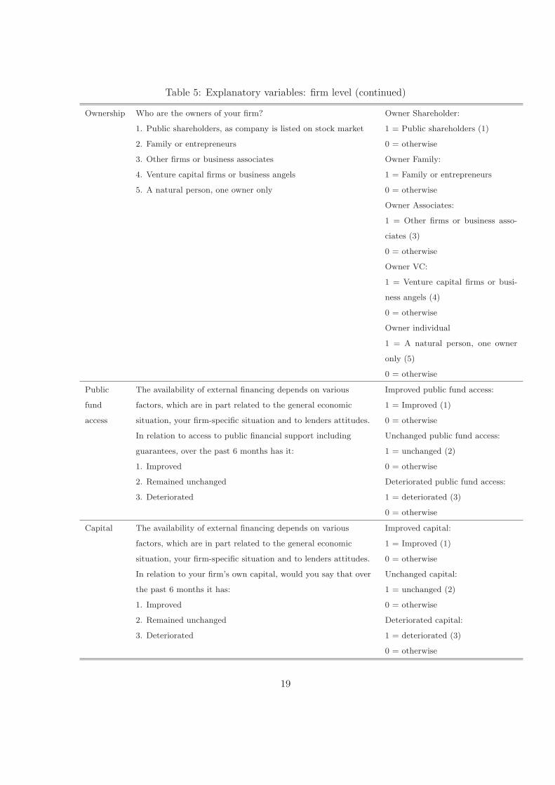
Table 5: Explanatory variables: firm level (continued)

Ownership Who are the owners of your firm? Owner Shareholder:

1. Public shareholders, as company is listed on stock market 1 = Public shareholders (1)

2. Family or entrepreneurs 0 = otherwise

3. Other firms or business associates Owner Family:

4. Venture capital firms or business angels 1 = Family or entrepreneurs

5. A natural person, one owner only 0 = otherwise

Owner Associates:

1 = Other firms or business asso-

ciates (3)

0 = otherwise

Owner VC:

1 = Venture capital firms or busi-

ness angels (4)

0 = otherwise

Owner individual

1 = A natural person, one owner

only (5)

0 = otherwise

Public The availability of external financing depends on various Improved public fund access:

fund factors, which are in part related to the general economic 1 = Improved (1)

access situation, your firm-specific situation and to lenders attitudes. 0 = otherwise

In relation to access to public financial support including Unchanged public fund access:

guarantees, over the past 6 months has it: 1 = unchanged (2)

1. Improved 0 = otherwise

2. Remained unchanged Deteriorated public fund access:

3. Deteriorated 1 = deteriorated (3)

0 = otherwise

Capital The availability of external financing depends on various Improved capital:

factors, which are in part related to the general economic 1 = Improved (1)

situation, your firm-specific situation and to lenders attitudes. 0 = otherwise

In relation to your firm’s own capital, would you say that over Unchanged capital:

the past 6 months it has: 1 = unchanged (2)

1. Improved 0 = otherwise

2. Remained unchanged Deteriorated capital:

3. Deteriorated 1 = deteriorated (3)

0 = otherwise

19

Table 6: Explanatory variables: macro level

GDP Change Gross domestic product, Constant prices, seasonally adjusted,

Eurostat

The percentage change in GDP over

the half year period for each survey

round

GB10Y Yield of the benchmark 10 Year Datastream Government Index 6 months average over the half year

period for each survey round

Log CDS

(Median)

Credit default swaps on banks bonds in each country Log of the price of the median bank

CDS for each period.

Private Debt

to GDP

Total stock of euro area private sector debt (loans and debt se-

curities) from Monetary Financial Institutions’ (MFIs excluding

ECB) balance sheets in each country, Gross domestic product

at market prices from ESA95 National Accounts, quarterly

The stock of debt at the end of each

half year in question divided by to-

tal GDP in that half year

Debt to Out-

put

Quarterly outstanding amount of loans to domestic non financial

corporations by NACE classification for the following categories

(with NACE definition in brackets):

Loans to each sector outstanding at

the end of each 6 month period

i)manufacturing, ii)construction, iii)wholesale and retail trade

(wholesale and retail trade, repair of motor vehicles and mo-

torcycles) iv) transport (transport and storage, information and

communication ) v) other (accommodation and food service ac-

tivities and education; human health and social work activities;

arts, entertainment and recreation; other service activities; ac-

tivities of households as employers; undifferentiated good)

divided by the output of that sector

in that year, for each country

Annual output of non financial corporations by NACE classi-

fication for the following categories (with NACE definition in

brackets):

i)manufacturing, ii)construction, iii)wholesale and retail trade

(wholesale and retail trade, repair of motor vehicles and mo-

torcycles) iv) transport (transport and storage, information and

communication ) v) other (accommodation and food service ac-

tivities and education; human health and social work activities;

arts, entertainment and recreation; other service activities; ac-

tivities of households as employers; undifferentiated good)

20

Table 7: Summary Statistics for Dependent and Macroeconomic Variables

Variable Mean Min Max Stand. Dev.

Loan Rejection 0.21 0.00 1.00 0.41

Perceived Deterioration 0.28 0.00 1.00 0.45

Demand Decrease 0.15 0.00 1.00 0.36

Interest Increase 0.45 0.00 1.00 0.50

Loan Size 0.19 0.00 1.00 0.39

GDP -0.15 -6.96 3.35 1.81

GB10Y 3.92 2.49 10.75 1.29

Log CDS (Median) 5.06 4.40 6.75 0.53

Private Debt to GDP 7.60 4.27 14.04 2.72

Debt to Output 77.43 6.52 429.43 102.42

21

Table 8: Firm Characteristics and Country Effects Relative to Germany

(1) (2) (3) (4) (5)Bank Perceived Demand Interest Loan SizeReject Deterioration Decrease Increase Increase

1 to 9 employees (d) 0.134∗∗∗ 0.0206 -0.0301∗∗∗ -0.0449 -0.0272(6.39) (1.21) (-2.70) (-1.37) (-1.54)

10 to 49 employees (d) 0.0465∗∗ -0.00502 -0.00686 -0.000228 0.0151(2.06) (-0.39) (-0.74) (-0.01) (0.76)

Profit Margin Fall (d) 0.000917 0.0370∗∗∗ -0.0162∗ 0.0397∗ -0.0119(0.05) (4.03) (-1.74) (1.95) (-0.77)

Subsidiary vs Independent (d) -0.0508∗∗ -0.0308 0.00471 -0.00657 0.0170(-2.24) (-1.63) (0.37) (-0.22) (0.80)

Age > 10 (d) -0.0759∗∗∗ -0.0220∗ 0.0212∗∗∗ 0.0342 0.00179(-4.20) (-1.68) (3.09) (1.14) (0.09)

Improved prospects (d) 0.0147 -0.0490∗∗ -0.00307 -0.0244 0.0171(0.55) (-2.56) (-0.21) (-0.85) (0.87)

Unchanged prospects (d) -0.0678∗∗∗ -0.119∗∗∗ -0.0152 -0.0214 -0.0223(-3.30) (-6.66) (-1.47) (-1.18) (-1.25)

Owner Shareholder (d) -0.00388 -0.0312 -0.00130 -0.00710 -0.000680(-0.09) (-1.62) (-0.08) (-0.15) (-0.02)

Owner Family (d) -0.0448∗ -0.0376∗∗∗ -0.00389 0.0186 -0.0176(-1.92) (-3.29) (-0.37) (0.89) (-1.10)

Owner Associates (d) -0.0244 -0.0462∗∗∗ -0.0106 -0.0587∗ -0.0474∗∗

(-0.65) (-2.85) (-0.86) (-1.73) (-2.29)Owner VC (d) 0.00321 0.0575 -0.0101 0.0527 -0.167∗∗∗

(0.07) (1.15) (-0.37) (0.69) (-11.14)Improved public fund access (d) -0.190∗∗∗ -0.217∗∗∗ 0.0106 -0.164∗∗∗ 0.0979∗∗∗

(-11.87) (-13.37) (0.64) (-6.85) (4.22)Unchanged public fund access (d) -0.182∗∗∗ -0.271∗∗∗ -0.0157∗ -0.136∗∗∗ 0.00539

(-9.16) (-18.26) (-1.65) (-7.58) (0.29)Improved capital (d) -0.130∗∗∗ -0.123∗∗∗ 0.139∗∗∗ -0.0416 0.0367

(-6.59) (-8.50) (8.84) (-1.50) (1.59)Unchanged capital (d) -0.0909∗∗∗ -0.131∗∗∗ 0.0214∗∗ -0.0348 -0.0184

(-4.21) (-9.17) (2.16) (-1.63) (-1.15)Austria (d) -0.0823 -0.00959 0.0101 -0.00803 -0.0471∗∗∗

(-1.33) (-0.50) (0.44) (-0.19) (-3.17)Belgium (d) -0.113∗∗∗ -0.0632∗∗∗ -0.00134 0.0500 -0.0263

(-4.30) (-3.35) (-0.08) (1.36) (-1.34)Spain (d) 0.0607∗∗ -0.0347 0.0325∗∗∗ 0.393∗∗∗ -0.0208

(2.10) (-1.10) (2.88) (16.69) (-1.32)Finland (d) -0.103∗∗∗ -0.0979∗∗∗ 0.0503∗∗∗ 0.0853∗∗∗ -0.0514∗∗∗

(-3.64) (-2.60) (3.57) (2.62) (-3.00)France (d) -0.0538 -0.0926∗∗∗ -0.0256∗∗ -0.00103 -0.0424∗∗∗

(-1.54) (-3.13) (-2.05) (-0.04) (-2.93)Greece (d) 0.156∗∗ 0.0782∗∗∗ 0.0112 0.268∗∗∗ -0.0706∗∗∗

(2.38) (3.37) (0.33) (10.34) (-3.10)Ireland (d) 0.0983∗ 0.117∗∗∗ 0.0315∗∗ 0.222∗∗∗ -0.110∗∗∗

(1.89) (2.83) (2.27) (5.49) (-6.07)Italy (d) 0.0117 -0.0708∗∗∗ -0.0307∗∗∗ 0.128∗∗∗ -0.0307

(0.38) (-5.20) (-2.58) (3.43) (-1.39)Netherlands (d) 0.171∗∗∗ 0.0198 0.0438∗∗ 0.0920 -0.0296

(3.69) (0.62) (2.00) (0.82) (-0.80)Portugal (d) 0.0700∗ 0.0250 0.00873 0.312∗∗∗ -0.112∗∗∗

(1.81) (0.56) (0.24) (11.22) (-4.40)

N 2,999 8,041 9,168 4,019 3,994r2 p 0.164 0.191 0.0474 0.148 0.0311

Marginal effects; t statistics in parentheses(d) for discrete change of dummy variable from 0 to 1∗

p < .1, ∗∗

p < .05, ∗∗∗

p < .01

22

Table 9: Stepwise Method of Including Country Variables(1) (2) (3) (4) (5)

Loan Perceived Demand Int Rate LoanRejection Deterioration Decrease Increase Increase

GDP Change -0.0115∗∗

(-2.47)GB10Y 0.0269∗∗∗ -0.0145∗∗

(3.93) (-2.25)Log CDS Spread (Median) 0.0730∗∗∗ 0.105∗∗∗

(4.77) (3.50)Private Debt to GDP 0.0120∗∗∗ 0.00804∗∗∗ 0.0403∗∗∗

(3.63) (5.23) (9.91)Debt to Output -0.000312∗∗ 0.000805∗∗

(-1.98) (2.23)1 to 9 employees (d) 0.145∗∗∗ 0.0295 -0.0129

(5.02) (1.60) (-0.65)10 to 49 employees (d) 0.0531∗∗ -0.000734 0.0253∗∗ 0.0292 0.0189

(2.27) (-0.05) (2.28) (1.16) (1.08)Profit Margin Fall (d) -0.00288 0.0435∗∗∗ -0.0104 0.0322 -0.0153

(-0.14) (3.08) (-1.14) (1.52) (-0.95)Subsidiary Dummy (d) -0.0486 -0.00572 -0.0148 -0.0269 0.0233

(-1.63) (-0.26) (-1.16) (-0.80) (0.86)Age > 10 (d) -0.0769∗∗∗ -0.0215 0.0259∗∗∗ 0.0413∗ 0.0151

(-3.49) (-1.44) (2.86) (1.88) (0.92)Improved prospects (d) -0.0581∗∗∗ 0.00372 -0.0516∗ 0.0249

(-2.98) (0.28) (-1.71) (1.06)Unchanged prospects (d) -0.0770∗∗∗ -0.124∗∗∗ -0.0190∗ -0.0414∗ -0.0144

(-3.00) (-8.03) (-1.80) (-1.68) (-0.77)Owner Shareholder (d) -0.0543 0.384∗∗∗

(-0.85) (2.89)Owner Family (d) -0.0988 0.00516 -0.00535 0.0292 0.253∗∗∗

(-1.44) (0.19) (-0.32) (0.71) (3.24)Owner Associates (d) -0.0710 -0.00784 -0.0101 -0.0527 0.306∗∗

(-1.20) (-0.26) (-0.55) (-1.14) (2.43)Owner VC (d) 0.121∗ -0.00977 0.0346

(1.92) (-0.28) (0.41)Improved public fund access (d) -0.182∗∗∗ -0.209∗∗∗ 0.0132 -0.144∗∗∗

(-10.46) (-14.00) (0.89) (-4.51)Unchanged public fund access (d) -0.188∗∗∗ -0.271∗∗∗ -0.00891 -0.122∗∗∗ -0.0834∗∗∗

(-9.78) (-20.12) (-0.94) (-5.60) (-3.68)Improved capital (d) -0.126∗∗∗ 0.140∗∗∗ -0.0563∗

(-5.31) (7.40) (-1.74)Unchanged capital (d) -0.108∗∗∗ -0.0153 0.0151 -0.0102 -0.0607∗∗∗

(-4.82) (-0.82) (1.34) (-0.41) (-3.03)

N 2,309 5,876 6,847 3,043 3,025R squared 0.151 0.178 0.0505 0.131 0.0281


p < .1, ∗∗

p < .05, ∗∗∗

p < .01

23

A Appendix

24

Table A1: Determinants of Loan Rejection

(1) (2) (3) (4) (5) (6)

1 to 9 employees (d) 0.129∗∗∗ 0.129∗∗∗ 0.136∗∗∗ 0.138∗∗∗ 0.134∗∗∗ 0.143∗∗∗

(6.23) (6.24) (6.36) (6.29) (5.52) (5.93)10 to 49 employees (d) 0.0434∗ 0.0437∗ 0.0456∗∗ 0.0454∗∗ 0.0482∗∗ 0.0528∗∗

(1.93) (1.93) (1.97) (2.03) (1.97) (2.12)Profit Margin Fall (d) 0.00420 0.00570 0.00426 0.00437 0.00248 -0.00392

(0.24) (0.33) (0.23) (0.24) (0.13) (-0.20)Subsidiary Dummy (d) -0.0430∗ -0.0434∗ -0.0519∗∗ -0.0480∗∗ -0.0374 -0.0479∗

(-1.75) (-1.75) (-2.08) (-2.00) (-1.50) (-1.87)Age > 10 (d) -0.0750∗∗∗ -0.0744∗∗∗ -0.0770∗∗∗ -0.0779∗∗∗ -0.0769∗∗∗ -0.0776∗∗∗

(-4.04) (-4.18) (-4.30) (-4.23) (-4.63) (-4.45)Improved prospects (d) 0.0177 0.0150 0.0189 0.0147 -0.000114 0.0152

(0.61) (0.52) (0.66) (0.50) (-0.00) (0.44)Unchanged prospects (d) -0.0766∗∗∗ -0.0766∗∗∗ -0.0710∗∗∗ -0.0722∗∗∗ -0.0739∗∗∗ -0.0635∗∗∗

(-3.64) (-3.65) (-3.31) (-3.25) (-3.01) (-2.62)Owner Shareholder (d) 0.00988 0.00890 0.0101 0.0216 0.0219 0.00513

(0.23) (0.21) (0.24) (0.53) (0.60) (0.14)Owner Family (d) -0.0364 -0.0387 -0.0411∗ -0.0345 -0.0266 -0.0331

(-1.55) (-1.59) (-1.73) (-1.49) (-1.20) (-1.49)Owner Associates (d) -0.0312 -0.0279 -0.0308 -0.0319 -0.00497 -0.0134

(-0.86) (-0.75) (-0.84) (-0.89) (-0.14) (-0.39)Owner VC (d) 0.0176 0.0239 0.0245 0.0136 0.0709 0.0668

(0.37) (0.50) (0.53) (0.32) (1.18) (1.12)Improved public fund access (d) -0.195∗∗∗ -0.196∗∗∗ -0.194∗∗∗ -0.194∗∗∗ -0.186∗∗∗ -0.182∗∗∗

(-12.01) (-11.68) (-11.27) (-11.52) (-10.71) (-10.24)Unchanged public fund access (d) -0.198∗∗∗ -0.199∗∗∗ -0.186∗∗∗ -0.186∗∗∗ -0.197∗∗∗ -0.187∗∗∗

(-10.44) (-11.05) (-9.70) (-8.95) (-10.80) (-8.76)Improved capital (d) -0.133∗∗∗ -0.133∗∗∗ -0.133∗∗∗ -0.126∗∗∗ -0.133∗∗∗ -0.126∗∗∗

(-6.39) (-6.18) (-6.49) (-6.64) (-5.61) (-5.42)Unchanged capital (d) -0.0924∗∗∗ -0.0950∗∗∗ -0.0946∗∗∗ -0.0824∗∗∗ -0.106∗∗∗ -0.108∗∗∗

(-4.23) (-4.30) (-4.30) (-3.83) (-3.76) (-3.99)GDP Change -0.0347∗∗∗ -0.0129

(-4.86) (-0.63)GB10Y 0.0290∗∗∗ 0.0137

(4.70) (0.73)Log CDS Spread (Median) 0.102∗∗∗ 0.0103

(6.23) (0.20)Private Debt to GDP 0.0141∗∗∗ 0.0103∗∗

(5.05) (1.97)Debt to Output 0.000854∗∗∗ 0.0000917

(3.24) (0.19)

N 2,999 2,999 2,941 2,999 2,353 2,309R squared 0.151 0.151 0.150 0.150 0.147 0.152


p < .1, ∗∗

p < .05, ∗∗∗

p < .01

25

Table A2: Perceived Deterioration in Loan availability

(1) (2) (3) (4) (5) (6)

1 to 9 employees (d) 0.0234 0.0219 0.0224 0.0263 0.0306 0.0291(1.38) (1.31) (1.32) (1.54) (1.40) (1.30)

10 to 49 employees (d) 0.0000401 -0.00149 -0.00236 0.00148 0.0000609 -0.000576(0.00) (-0.13) (-0.20) (0.13) (0.00) (-0.04)

Profit Margin Fall (d) 0.0374∗∗∗ 0.0373∗∗∗ 0.0364∗∗∗ 0.0377∗∗∗ 0.0436∗∗∗ 0.0425∗∗∗

(3.69) (3.69) (3.74) (4.03) (3.52) (3.62)Subsidiary Dummy (d) -0.0169 -0.0180 -0.0213 -0.0200 -0.00279 -0.00505

(-0.92) (-0.97) (-1.12) (-1.08) (-0.15) (-0.28)Age > 10 (d) -0.0135 -0.0142 -0.0223∗ -0.0151 -0.0157 -0.0218∗

(-1.11) (-1.17) (-1.73) (-1.25) (-1.33) (-1.68)Improved prospects (d) -0.0436∗∗ -0.0445∗∗ -0.0459∗∗ -0.0448∗∗ -0.0567∗∗ -0.0574∗∗

(-2.17) (-2.19) (-2.20) (-2.15) (-2.32) (-2.29)Unchanged prospects (d) -0.118∗∗∗ -0.119∗∗∗ -0.115∗∗∗ -0.118∗∗∗ -0.128∗∗∗ -0.124∗∗∗

(-6.49) (-6.42) (-6.02) (-6.15) (-6.09) (-5.76)Owner Shareholder (d) -0.0365∗ -0.0406∗∗ -0.0458∗∗ -0.0328 -0.0407∗∗ -0.0498∗∗

(-1.86) (-2.17) (-2.43) (-1.56) (-2.12) (-2.54)Owner Family (d) -0.0375∗∗∗ -0.0406∗∗∗ -0.0468∗∗∗ -0.0353∗∗∗ -0.0364∗∗∗ -0.0463∗∗∗

(-3.36) (-3.68) (-4.45) (-3.02) (-2.89) (-4.21)Owner Associates (d) -0.0658∗∗∗ -0.0641∗∗∗ -0.0683∗∗∗ -0.0647∗∗∗ -0.0488∗∗∗ -0.0580∗∗∗

(-4.48) (-4.28) (-4.62) (-4.51) (-3.30) (-3.50)Owner VC (d) 0.0446 0.0462 0.0432 0.0455 0.0699 0.0642



(-16.03) (-16.96) (-15.98) (-16.36) (-18.49) (-16.68)Improved capital (d) -0.117∗∗∗ -0.116∗∗∗ -0.115∗∗∗ -0.119∗∗∗ -0.124∗∗∗ -0.119∗∗∗

(-7.73) (-7.61) (-7.32) (-8.19) (-6.25) (-5.85)Unchanged capital (d) -0.132∗∗∗ -0.132∗∗∗ -0.133∗∗∗ -0.131∗∗∗ -0.144∗∗∗ -0.142∗∗∗

(-9.92) (-9.84) (-9.74) (-9.99) (-8.55) (-8.50)GDP Change -0.0228∗∗∗ -0.00423

(-2.86) (-0.24)GB10Y 0.0226∗∗∗ -0.00853

(3.51) (-0.41)Log CDS Spread (Median) 0.0801∗∗∗ 0.0762

(3.60) (1.64)Private Debt to GDP 0.00714 0.000582

(1.49) (0.11)Debt to Output 0.000541∗∗ 0.000211

(2.52) (0.60)

N 8,041 8,041 7,783 8,041 6,056 5,876R squared 0.183 0.184 0.183 0.182 0.177 0.178


p < .1, ∗∗

p < .05, ∗∗∗

p < .01

26

Table A3: Decrease in Loan Demand

(1) (2) (3) (4) (5) (6)

1 to 9 employees (d) -0.0301∗∗∗ -0.0301∗∗∗ -0.0339∗∗∗ -0.0282∗∗ -0.0294∗∗∗ -0.0308∗∗∗

(-2.66) (-2.66) (-3.08) (-2.48) (-2.90) (-3.21)10 to 49 employees (d) -0.00589 -0.00599 -0.0105 -0.00469 -0.00299 -0.00679

(-0.61) (-0.62) (-1.15) (-0.48) (-0.33) (-0.79)Profit Margin Fall (d) -0.0154∗ -0.0151∗ -0.0144 -0.0173∗∗ -0.00772 -0.0102

(-1.81) (-1.73) (-1.60) (-1.96) (-0.92) (-1.20)Subsidiary Dummy (d) 0.0126 0.0118 0.0106 0.00982 -0.0128 -0.0147

(0.92) (0.86) (0.79) (0.73) (-1.05) (-1.18)Age > 10 (d) 0.0263∗∗∗ 0.0263∗∗∗ 0.0272∗∗∗ 0.0247∗∗∗ 0.0264∗∗∗ 0.0256∗∗∗

(3.97) (3.95) (3.93) (3.64) (3.57) (3.21)Improved prospects (d) -0.00281 -0.00393 -0.00449 -0.00111 -0.00192 0.00382

(-0.20) (-0.28) (-0.31) (-0.08) (-0.12) (0.23)Unchanged prospects (d) -0.0176∗ -0.0181∗ -0.0179∗ -0.0155 -0.0227∗∗ -0.0189∗

(-1.72) (-1.75) (-1.71) (-1.49) (-2.07) (-1.73)Owner Shareholder (d) -0.00131 -0.000938 0.00242 -0.00229 0.00961 0.00611

(-0.08) (-0.06) (0.15) (-0.14) (0.49) (0.32)Owner Family (d) -0.00349 -0.00304 -0.00474 -0.00479 0.00423 0.000219

(-0.33) (-0.28) (-0.42) (-0.44) (0.31) (0.02)Owner Associates (d) -0.0136 -0.0125 -0.00949 -0.0152 -0.000211 -0.00500

(-1.10) (-0.98) (-0.78) (-1.23) (-0.01) (-0.33)Owner VC (d) -0.0117 -0.0106 -0.00685 -0.0133 -0.00346 -0.00470

(-0.44) (-0.39) (-0.25) (-0.50) (-0.11) (-0.15)Improved public fund access (d) 0.00736 0.00652 0.00941 0.0124 0.00719 0.0131

(0.46) (0.40) (0.55) (0.75) (0.40) (0.68)Unchanged public fund access (d) -0.0221∗∗ -0.0227∗∗ -0.0182∗ -0.0161∗ -0.0182∗ -0.00895

(-2.34) (-2.39) (-1.92) (-1.69) (-1.66) (-0.85)Improved capital (d) 0.142∗∗∗ 0.141∗∗∗ 0.142∗∗∗ 0.143∗∗∗ 0.134∗∗∗ 0.139∗∗∗

(8.01) (8.03) (7.72) (8.38) (6.22) (6.49)Unchanged capital (d) 0.0198∗∗ 0.0193∗∗ 0.0179∗ 0.0201∗∗ 0.0135 0.0152

(2.02) (1.97) (1.83) (2.04) (1.25) (1.41)GDP Change -0.00977∗∗∗ -0.0144∗

(-2.81) (-1.81)GB10Y 0.00573 -0.00448

(1.61) (-0.45)Log CDS Spread (Median) 0.0319∗∗∗ 0.00433

(2.76) (0.19)Private Debt to GDP 0.00634∗∗∗ 0.00758∗∗∗

(4.17) (3.08)Debt to Output -0.0000113 -0.000293

(-0.09) (-1.44)

N 9,168 9,168 8,870 9,168 7,063 6,847R squared 0.0422 0.0416 0.0436 0.0440 0.0432 0.0506


p < .1, ∗∗

p < .05, ∗∗∗

p < .01

27

Table A4: Interest Rate Increase

(1) (2) (3) (4) (5) (6)

1 to 9 employees (d) -0.0581∗ -0.0598∗∗ -0.0610∗ -0.0377 -0.0489 -0.0349(-1.86) (-2.00) (-1.87) (-1.18) (-1.47) (-0.98)

10 to 49 employees (d) -0.00727 -0.00934 -0.00748 -0.00328 -0.0109 -0.00506(-0.34) (-0.44) (-0.34) (-0.14) (-0.46) (-0.20)

Profit Margin Fall (d) 0.0681∗∗∗ 0.0690∗∗∗ 0.0553∗∗∗ 0.0530∗∗ 0.0577∗∗ 0.0322(3.14) (3.06) (2.59) (2.57) (2.29) (1.34)

Subsidiary Dummy (d) 0.00189 -0.000361 -0.0170 -0.0186 -0.00791 -0.0260(0.06) (-0.01) (-0.61) (-0.60) (-0.25) (-0.82)

Age > 10 (d) 0.0454 0.0454 0.0297 0.0328 0.0531∗ 0.0402(1.47) (1.44) (0.95) (1.11) (1.66) (1.26)

Improved prospects (d) -0.0520∗∗ -0.0562∗∗ -0.0397 -0.0392 -0.0864∗∗∗ -0.0509∗

(-1.97) (-2.01) (-1.40) (-1.33) (-2.97) (-1.70)Unchanged prospects (d) -0.0534∗∗∗ -0.0553∗∗∗ -0.0381∗ -0.0327∗ -0.0721∗∗∗ -0.0410∗

(-3.04) (-2.79) (-1.95) (-1.67) (-3.22) (-1.79)Owner Shareholder (d) 0.0422 0.0335 0.0165 0.0423 0.0535 0.00679

(0.78) (0.68) (0.35) (0.86) (1.00) (0.14)Owner Family (d) 0.0657∗∗∗ 0.0587∗∗∗ 0.0453∗∗ 0.0502∗∗ 0.0654∗∗∗ 0.0363∗

(2.79) (2.68) (2.27) (2.41) (2.83) (1.65)Owner Associates (d) -0.0153 -0.00957 -0.0242 -0.0341 0.00503 -0.0480

(-0.37) (-0.24) (-0.71) (-0.99) (0.11) (-1.21)Owner VC (d) 0.0898 0.0984 0.102 0.0688 0.0729 0.0380



(-10.11) (-9.95) (-8.78) (-7.63) (-7.41) (-5.48)Improved capital (d) -0.0625∗∗ -0.0619∗∗ -0.0589∗∗ -0.0431 -0.0718∗∗ -0.0568∗

(-1.98) (-2.05) (-2.08) (-1.50) (-2.32) (-1.84)Unchanged capital (d) -0.0259 -0.0304 -0.0247 -0.0112 -0.0225 -0.00966

(-1.16) (-1.43) (-1.18) (-0.52) (-0.84) (-0.36)GDP Change -0.0700∗∗∗ -0.0241

(-2.97) (-1.54)GB10Y 0.0614∗∗ -0.0251

(2.28) (-1.62)Log CDS Spread (Median) 0.278∗∗∗ 0.128∗∗∗

(5.25) (2.59)Private Debt to GDP 0.0495∗∗∗ 0.0372∗∗∗

(8.82) (6.03)Debt to Output 0.00170∗∗∗ 0.000810∗

(3.17) (1.92)

N 4,019 4,019 3,954 4,019 3,092 3,043R squared 0.0939 0.0939 0.119 0.129 0.0839 0.132


p < .1, ∗∗

p < .05, ∗∗∗

p < .01

28

Table A5: Loan Size Increase

(1) (2) (3) (4) (5) (6)

1 to 9 employees (d) -0.0300∗ -0.0280 -0.0311∗ -0.0315∗ -0.0105 -0.0122(-1.76) (-1.63) (-1.81) (-1.85) (-0.60) (-0.68)

10 to 49 employees (d) 0.0116 0.0125 0.0105 0.0117 0.0214 0.0194(0.59) (0.64) (0.53) (0.59) (0.94) (0.83)

Profit Margin Fall (d) -0.00963 -0.00870 -0.00843 -0.00972 -0.0145 -0.0155(-0.60) (-0.54) (-0.51) (-0.61) (-0.72) (-0.76)

Subsidiary Dummy (d) 0.0177 0.0180 0.0138 0.0188 0.0309 0.0237(0.86) (0.88) (0.69) (0.89) (1.27) (0.97)

Age > 10 (d) 0.00319 0.00394 0.00582 0.00372 0.0149 0.0131(0.16) (0.20) (0.29) (0.18) (0.70) (0.59)

Improved prospects (d) 0.0158 0.0142 0.0203 0.0170 0.0185 0.0272(0.83) (0.74) (1.09) (0.89) (0.77) (1.14)

Unchanged prospects (d) -0.0243 -0.0260 -0.0264 -0.0239 -0.0152 -0.0123(-1.34) (-1.44) (-1.47) (-1.33) (-0.79) (-0.66)

Owner Shareholder (d) -0.00393 0.00421 0.000668 -0.00694 0.00898 0.00594(-0.13) (0.14) (0.02) (-0.24) (0.26) (0.17)

Owner Family (d) -0.0231 -0.0188 -0.0191 -0.0238 -0.0196 -0.0202(-1.48) (-1.19) (-1.22) (-1.54) (-1.16) (-1.16)

Owner Associates (d) -0.0478∗∗ -0.0475∗∗ -0.0442∗∗ -0.0481∗∗ -0.0408 -0.0413∗

(-2.22) (-2.18) (-1.99) (-2.28) (-1.61) (-1.64)Owner VC (d) -0.167∗∗∗ -0.166∗∗∗ -0.166∗∗∗ -0.166∗∗∗ -0.167∗∗∗ -0.167∗∗∗

(-10.42) (-10.81) (-10.50) (-10.62) (-8.69) (-9.40)Improved public fund access (d) 0.0949∗∗∗ 0.0937∗∗∗ 0.0964∗∗∗ 0.0945∗∗∗ 0.0769∗∗∗ 0.0803∗∗∗

(4.16) (4.19) (4.20) (4.20) (3.21) (3.36)Unchanged public fund access (d) 0.00583 0.00479 0.00279 0.00485 -0.0121 -0.00959

(0.30) (0.24) (0.14) (0.26) (-0.51) (-0.42)Improved capital (d) 0.0371 0.0357 0.0391 0.0370 0.0400 0.0406

(1.59) (1.54) (1.62) (1.58) (1.55) (1.52)Unchanged capital (d) -0.0189 -0.0166 -0.0162 -0.0202 -0.0246 -0.0210

(-1.15) (-1.01) (-0.95) (-1.20) (-1.34) (-1.13)GDP Change 0.00954∗ -0.0234∗

(1.66) (-1.95)GB10Y -0.0186∗∗∗ -0.0346∗∗∗

(-3.22) (-3.04)Log CDS Spread (Median) -0.0340∗∗ 0.0383

(-2.15) (1.30)Private Debt to GDP -0.00192 -0.00244

(-0.65) (-0.86)Debt to Output -0.000527∗∗ -0.000402∗

(-2.16) (-1.79)

N 3,994 3,994 3,930 3,994 3,074 3,025R squared 0.0245 0.0269 0.0263 0.0241 0.0275 0.0300


p < .1, ∗∗

p < .05, ∗∗∗

p < .01

29

Documents

4/RT/12 Firm Credit in Europe: A Tale of Three Crises