4D N =1 Superconformal Bootstrap

Andy StergiouCERN

2

Unknown 4D SCFT?

Is there an SCFT here?

1 1.1 1.2 1.3 1.4 1.5 1.6 1.7 1.8 1.9 22

3

4

5

� ¯��= 2��

��

�¯��

Fig. 1: Upper bound on the allowed dimension of the operator �̄� (the leading relevant nonchiral

scalar singlet) as a function of the dimension of �. The generalized free theory dashed line

�¯�� = 2�� is also shown. The shaded area is excluded. If we assume that �2 is not in the

spectrum then everything to the left of the dotted line at �� = 1.407, which is the position of the

kink, is excluded. Here we use ⇤ = 21.

this bound necessarily does not contain any scalar superconformal primaries of dimension 2, i.e. �

cannot be charged under any global symmetries.

Next we recompute this bound imposing the additional condition that the chiral �2 operator

does not appear in the �⇥ � OPE. This condition has the e↵ect of excluding all points to the left

of the dotted vertical line in Fig. 1. The region to the right remains the same. In other words, it

imposes the strict lower bound �� � 1.407, causing the mild kink to turn into a sharp corner.

One can see that this had to be the case by considering bounds on the OPE coe�cient of the

operator �2, shown in Fig. 2. The lower bound on ��2

disappears exactly at �� = 1.407. Thus,

Fig. 2 makes it clear that if we demand ��2

= 0, implying that �2 is not in the spectrum, then all

points to the left of �� = 1.407 must be excluded. Our general bound is also compatible with the

results of [9], which found that the �2 operator was absent in approximate solutions to crossing

symmetry living on the boundary of the allowed region to the right of the kink.

In Fig. 3 we show an upper bound on the OPE coe�cient �¯�� of an operator whose dimension

saturates the bound in Fig. 1. Without any additional assumptions the upper bound attains a

minimum at precisely the location of the kink, occuring at �¯�� ' 0.905. If we further impose the

absence of �2, then all points to the left of the dotted vertical line in Fig. 3 are excluded.

Next we would like to ask the question: if there is an SCFT living near the kink with the chiral

ring relation �2 = 0, does it contain a stress-energy tensor? In other words, could it correspond

to a local SCFT? In Fig. 4 we assume �2 = 0 and place an upper bound on the leading spin-1

superconformal primary V in the �̄⇥ � OPE, again at ⇤ = 21. We see that the bound on �V

approaches 3 as �� approaches its minimum value. Thus, the U(1)R current multiplet VR is

3

To be optimistic, let’s give it a name: minimal 4D SCFTN = 1

3

Outline

The bootstrap philosophy

The 4D superconformal bootstrap

Basic facts about CFTs

4

Operators in CFTs

In CFTs operators can be grouped into primaries and descendants:

Kµ (O(0)) = 0 or Kµ (O(0)) ! 0.

Descendants are derivatives of primaries.

In CFTs correlation functions of primary operators are severely constrained:

⟨O1(x1)O2(x2)O3(x3)⟩ =C123

(x122)12 (∆1+∆2−∆3) (x232)

12 (∆2+∆3−∆1) (x132)

12 (∆1+∆3−∆2)

.

⟨O(x)O(0)⟩ = CO(x2)∆O

, ⟨O1(x)O2(0)⟩ = 0 ,

5

These constraints arise from the fact that with two or three points in space one cannot write down any conformally invariant quantities.

Operators in CFTs

This is not so with four points:

u =x122x342

x132x242v =

x142x232

x132x242.and

The four-point function of primary operators in CFTs is given in terms of a function of u and v:

⟨O1(x1)O2(x2)O3(x3)O4(x4)⟩ =!x242

x142

" 12 (∆1−∆2) !

x142

x132

" 12 (∆3−∆4) g(u, v)

(x122)12 (∆1+∆2) (x342)

12 (∆3+∆4)

.

6

Conformal Blocks

In remarkable work Dolan and Osborn computed this function for scalar external operators in 2001.

O1

O2

O3

O4

O

Using the operator product expansion,

one can view the four point function as a sum over contributions of the form

The exchanged operators can be primaries or descendants.

C12O C34O

O1(x) × O2(0) =!

O

C12O

(x2)12 (∆1+∆2−∆O )

O(0)

g(u, v)

7

Dolan and Osborn managed to resum the contributions of the descendants of any given primary, and determine the resulting sums.

Conformal Blocks

As a result,

g(u, v) =!

OC12OC34O gO (u, v).

Conformalblocks

The four-point function follows from knowing all possible exchanged primary operators and OPE coefficients.

The conformal blocks depend on the scaling dimension and the spin of the exchanged primary operators.

8

Crossing Symmetry

It must be that

O4

O1

O2

O3

O4

OC12O

O1

O2

O3

C34O=

O ′C14O′ C23O′

We are now ready to set up the constraint used in the conformal bootstrap program.

This simple constraint provides the basis of all bootstrap analyses.

!

O

!

O′

(kin. fac.) ×!

OC12OC34O gO (u, v) = (kin. fac.) ×

!

O′C14O′C23O′ gO′ (v, u)

9

How To Extract Information

Let’s take the simple case of a CFT containing a scalar operator φ.

Its four-point function can be expressed in two ways:

Equality of the right-hand sides gives

⟨φ(x1)φ(x2)φ(x3)φ(x4)⟩ =1

(x122x342)∆φ!

OC 2φφOgO (u, v),

!

OC 2φφOFO (u, v) = 0, FO (u, v) = u−∆φ gO (u, v) − v−∆φ gO (v, u).

⟨φ(x1)φ(x2)φ(x3)φ(x4)⟩ =1

(x142x232)∆φ!

OC 2φφOgO (v, u).

10

If our theory is unitary then

How To Extract Information!

OC 2φφOFO (u, v) = 0, FO (u, v) = u−∆φ gO (u, v) − v−∆φ gO (v, u).

C 2φφO > 0.

Let us separate the contributions of the identity operator and of another operator of interest:

We can act on this equation with a linear functional α :

C 2φφO0α(FO0 ) = −α(F1) −!

O!1,O0C 2φφOα(FO ).

C 2φφO0FO0 = −F1 −!

O!1,O0C 2φφOFO .

O0

11

We can demand

How To Extract Information

C 2φφO0α(FO0 ) = −α(F1) −!

O!1,O0C 2φφOα(FO ).

α(FO0 ) = 1 and α(FO ) ≥ 0.Then,

−α(F1)If we now minimize we have an upper bound on CφφO0 !

With this method we can obtain rigorous bounds on the interaction strength of CFTs!

This is an optimization problem, solved numerically on the computer.

C 2φφO0

= −α(F1) −!

O!1,O0

(positive × positive) ≤ −α(F1).

12

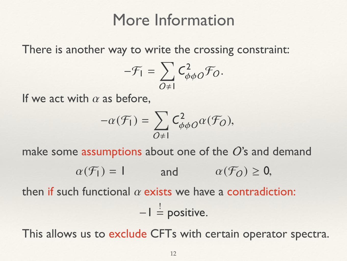
More Information

There is another way to write the crossing constraint:

−F1 =!

O!1C 2φφOFO .

If we act with as before,

−α(F1) =!

O!1C 2φφOα(FO ),

α

make some assumptions about one of the ’s and demand

α(F1) = 1 α(FO ) ≥ 0,and

then if such functional exists we have a contradiction:α

−1 != positive.

O

This allows us to exclude CFTs with certain operator spectra.

13

Superconformal Theories

Superconformal theories have fermionic generators:

{Sα, S̄α̇} = 2σµαα̇Kµ .

{Qα, Q̄α̇} = 2σµαα̇Pµ ,

There are superconformal primary operators:and S̄α̇ (O(0)) = 0 ,Sα (O(0)) = 0

and superconformal descendants which are “half” a derivative on a superconformal primary:

OSD = Q(OSP) or Q̄(OSP).

Every superconformal multiplet contains a single superconformal primary and many superconformal descendants that contain conformal primaries.

14

Chiral Bootstrap

Assume we have a 4D SCFT that contains a chiral operator φ.

⟨φ(x1)φ̄(x2)φ(x3)φ̄(x4)⟩

⟨φ(x1)φ̄(x2)φ(x3)φ̄(x4)⟩

We take the superconformal primary of the multiplet and look at the four-point function in two ways:

N = 1

15

We obtain the crossing relations!

O∈φ̄×φ|CO |2G∆,ℓ (u, v) =

"uv

#∆φ !

O∈φ̄×φ|CO |2G∆,ℓ (v, u).

!

O∈φ̄×φ|CO |2G∆,ℓ (u, v) =

"uv

#∆φ !

O∈φ×φ|CO |2g∆,ℓ (v, u).

Chiral Bootstrap

G∆,ℓ = g∆,ℓ + c1 g∆+1,ℓ−1 + c2 g∆+1,ℓ+1 + c1c2 g∆+2,ℓ,

c1 =∆ − ℓ − 24(∆ − ℓ − 1) , c2 =

∆ + ℓ

4(∆ + ℓ + 1).

For the superconformal block we find

with

(Poland & Simmons-Duffin, 2010)

16

Results

1 1.1 1.2 1.3 1.4 1.5 1.6 1.7 1.8 1.9 22

3

4

5

� ¯��= 2��

��

�¯��

Fig. 1: Upper bound on the allowed dimension of the operator �̄� (the leading relevant nonchiral

scalar singlet) as a function of the dimension of �. The generalized free theory dashed line

�¯�� = 2�� is also shown. The shaded area is excluded. If we assume that �2 is not in the

spectrum then everything to the left of the dotted line at �� = 1.407, which is the position of the

kink, is excluded. Here we use ⇤ = 21.

this bound necessarily does not contain any scalar superconformal primaries of dimension 2, i.e. �

cannot be charged under any global symmetries.

Next we recompute this bound imposing the additional condition that the chiral �2 operator

does not appear in the �⇥ � OPE. This condition has the e↵ect of excluding all points to the left

of the dotted vertical line in Fig. 1. The region to the right remains the same. In other words, it

imposes the strict lower bound �� � 1.407, causing the mild kink to turn into a sharp corner.

One can see that this had to be the case by considering bounds on the OPE coe�cient of the

operator �2, shown in Fig. 2. The lower bound on ��2

disappears exactly at �� = 1.407. Thus,

Fig. 2 makes it clear that if we demand ��2

= 0, implying that �2 is not in the spectrum, then all

points to the left of �� = 1.407 must be excluded. Our general bound is also compatible with the

results of [9], which found that the �2 operator was absent in approximate solutions to crossing

symmetry living on the boundary of the allowed region to the right of the kink.

In Fig. 3 we show an upper bound on the OPE coe�cient �¯�� of an operator whose dimension

saturates the bound in Fig. 1. Without any additional assumptions the upper bound attains a

minimum at precisely the location of the kink, occuring at �¯�� ' 0.905. If we further impose the

absence of �2, then all points to the left of the dotted vertical line in Fig. 3 are excluded.

Next we would like to ask the question: if there is an SCFT living near the kink with the chiral

ring relation �2 = 0, does it contain a stress-energy tensor? In other words, could it correspond

to a local SCFT? In Fig. 4 we assume �2 = 0 and place an upper bound on the leading spin-1

superconformal primary V in the �̄⇥ � OPE, again at ⇤ = 21. We see that the bound on �V

approaches 3 as �� approaches its minimum value. Thus, the U(1)R current multiplet VR is

3

(Poland & AS, 2015)

(Poland, Simmons-Duffin & Vichi, 2011)

1 1.1 1.2 1.3 1.4 1.5 1.6 1.7 1.8 1.9 20

1

2

3

��

��2

Fig. 2: Lower and upper bounds on the OPE coe�cient of the operator �2 in the � ⇥ � OPE.

The vertical dotted line is at �� = 1.407 and the horizontal dashed line is at the free theory value

��2

=p2. The shaded area is excluded. Here we use ⇤ = 21.

1 1.1 1.2 1.3 1.4 1.5 1.6 1.7 1.8 1.9 20.85

0.9

0.95

1

1.05

��

�¯��

Fig. 3: Upper bound on the OPE coe�cient of an operator �̄� with dimension �(bound)

¯��as a

function of the dimension of �. Here we do not assume that �̄� is the scalar with the lowest

dimension in the OPE �̄⇥ �. The shaded area is excluded. In this plot we use ⇤ = 21.

required to be in the spectrum at this point.

Note that for su�ciently small �� the bound excludes the line that would correspond to a

generalized free theory with �V = 2��+1. This is natural, as our assumption that �2 is absent is

4

17

Results

1.3 1.35 1.4 1.45 1.5 1.55 1.6 1.65 1.7 1.75 1.8 1.85 1.9 1.95 2

2

2.5

3

3.5

4

4.5

�

¯��=

2

��

��

�

¯��

Fig.1: Plot of the bound on the dimension of

¯�� as a function of the dimension of �. The shaded

area is excluded. Everything to the left of the vertical dotted line at d� = 1.407 is excluded due

to the assumption that there is no �2

operator. The generalized free theory dashed line �S = 2d�

is also shown. In this plot we use nmax

= 11.

1

(φ2 = 0)

(Poland & AS, 2015)

Assuming creates a sharp corner!φ2 = 0

18

Results

1 1.1 1.2 1.3 1.4 1.5 1.6 1.7 1.8 1.9 20

1

2

3

��

��2

Fig. 2: Lower and upper bounds on the OPE coe�cient of the operator �2 in the � ⇥ � OPE.

The vertical dotted line is at �� = 1.407 and the horizontal dashed line is at the free theory value

��2

=p2. The shaded area is excluded. Here we use ⇤ = 21.

1 1.1 1.2 1.3 1.4 1.5 1.6 1.7 1.8 1.9 20.85

0.9

0.95

1

1.05

��

�¯��

Fig. 3: Upper bound on the OPE coe�cient of an operator �̄� with dimension �(bound)

¯��as a

function of the dimension of �. Here we do not assume that �̄� is the scalar with the lowest

dimension in the OPE �̄⇥ �. The shaded area is excluded. In this plot we use ⇤ = 21.

required to be in the spectrum at this point.

Note that for su�ciently small �� the bound excludes the line that would correspond to a

generalized free theory with �V = 2��+1. This is natural, as our assumption that �2 is absent is

4

(Poland & AS, 2015)

1.3 1.4 1.5 1.6 1.7 1.8 1.9 24

4.5

5

5.5

6

��

�V 0

Fig. 5: Upper bound on the dimension of the second superconformal primary vector operator in

the OPE �̄⇥ � as a function of the dimension of �, assuming that the first vector has dimension

3. the shaded area is excluded. everything to the left of the vertical dotted line at �� = 1.407 is

excluded due to the assumption that there is no �2 operator. In this plot we use ⇤ = 21.

1 1.1 1.2 1.3 1.4 1.5 1.6 1.7 1.8 1.9 20

0.05

0.1

��

c

Fig. 6: Lower bound on the central charge as a function of the dimension of �. The shaded area

is excluded. For the strongest bound (thick line) we use ⇤ = 29, while for the weaker bounds

(thin lines) we use ⇤ = 21, 23, 25, 27 (from bottom to top). The dotted line is at �� = 1.407.

at ⇤ = 21 and �V 0 � 4.1 (�V 0 � 4.2 seems to be excluded at ⇤ = 35). Unfortunately, the location

has not yet completely converged at ⇤ = 35, but there is a striking linear relation between �� and

c, given approximately by c ⇡ 1.454���1.965. Moreover, as we increase ⇤ the rate of convergence

appears to be well-described by a fit that is linear in 1/⇤ (similar to the fit done in [15]),

{��(⇤), c(⇤)} ⇡⇢1.428� 0.441

⇤, 0.111� 0.642

⇤

�. (2.2)

These fits are shown in Fig. 9. While these extrapolations should be taken with a grain of salt, it

is intriguing that the minimal point may be converging to c(1) = 1/9 or c(1)/cfree

= 8/3. If the

minimal 4D N = 1 SCFT exists and has a simple rational central charge, this is our current best

6

19

Results

1.3 1.4 1.5 1.6 1.7 1.8 1.9 23

4

5

�V= 2�� +

1

(1.486, 3.972)

��

�V

Fig. 4: Upper bound on the dimension of the leading superconformal primary vector operator in

the OPE �̄⇥ � as a function of the dimension of �. The shaded area is excluded. Everything to

the left of the vertical dotted line at �� = 1.407 is excluded due to the assumption that there is

no �2 operator. The generalized free theory dashed line �V = 2�� + 1 as well as its intersection

with the bound are also shown. In this plot we use ⇤ = 21.

not true in a generalized free theory. On the other hand, when �� � 3/2, the contribution in the

sum rule corresponding to the chiral �2 operator is identical to one contained in the unprotected

scalar contributions in � ⇥ �. Thus, we expect the generalized free line should be allowed for

�� � 3/2. Here we see that it crosses this line at �� ⇠ 1.486, compatible with this expectation.

Now that we have established the existence of a U(1)R current multiplet, we can assume it to

be in the spectrum and place an upper bound on the second spin-1 operator V 0. The result is

shown in Fig. 5. We see that �V 0 . 4.25 at the minimum value of ��.

We can also compute general lower bounds on the central charge c, using that the OPE

coe�cient �2

VR= �2

�/72c. Here our normalization is such that cfree

= 1/24 for a free chiral

multiplet. Similar bounds were computed in [16]. Here these bounds are shown in Fig. 6 for

⇤ = 21, 23, . . . , 29. As in [16], these bounds drop very sharply as �� ! 1 so as to be compatible

with the free theory value cfree

= 1/24.

We can also impose a gap until the second spin-1 dimension �V 0 and find upper bounds on

c for each value of the gap. These bounds are shown in Fig. 7 at ⇤ = 21, where we have also

imposed that there is no �2 operator. We see that the upper and lower bounds meet at the

minimum value of ��, essentially uniquely fixing the central charge at this point, with c ' .081 at

⇤ = 21.

On the other hand, as seen in Fig. 6, our bounds have not yet converged, so the location of

this unique point in {��, c} space will change somewhat at larger values of ⇤. We have explored

the location of this point up to ⇤ = 35, shown in Fig. 8. Our strongest bound is �� � 1.415 at

⇤ = 35. In this plot we also compare these points to the upper and lower bounds on c computed

5

(Poland & AS, 2015)

In superconformal theories the stress-energy tensor appears in a vector multiplet known as the Ferrara–Zumino multiplet.

The Ferrara–Zumino multiplet has dimension exactly 3.

(φ2 = 0)

20

Results

1.38 1.4 1.42 1.44 1.46 1.48 1.5 1.52 1.540

0.1

0.2

0.3

0.4

��

c

Fig. 7: Lower and upper bounds on the central charge as a function of the dimension of �,

with the assumption that there is no �2 operator and all vector operators but the first one

obey �Vother

� 4.1 (thick upper bound line). The thinner upper bound lines correspond to

�Vother

� 3.1, 3.3, 3.5, 3.7, 3.9, 4 (from left to right). The shaded area is excluded. In this plot we

use ⇤ = 21.

1.404 1.406 1.408 1.41 1.412 1.414 1.416 1.4180.07

0.08

0.09

0.1

��

c

Fig. 8: Lower and upper bounds on the central charge as a function of the dimension of �, with

the assumptions that there is no �2 operator and that all vector operators but the first one obey

�Vother

� 4.1. The shaded area is excluded. Here we use ⇤ = 21 for the bounds. The green points

are allowed points closest to the corresponding lower bound for ⇤ = 21, 23, . . . , 35 (from left to

right).

conjecture.2 It is also possible that �� is converging to the rational value ��(1) = 10/7.

We finish with some preliminary explorations of the higher spectrum. In Fig. 10 we show the

2

If this conjecture is true, the bounds of [24] would then imply that

1

18

a 1

6

.

7

(Poland & AS, 2015)

We can also get upper bounds on the central charge.

These results basically determine the central charge!

(φ2 = 0)

21

Results

Increasing the order of the functional considered gives us stronger bounds.

0 0.01 0.02 0.03 0.04 0.051.4

1.41

1.42

1.43

1.44

1

⇤

��

0 0.01 0.02 0.03 0.04 0.050.07

0.08

0.09

0.1

0.11

0.12

1

⇤

c

Fig. 9: Linear extrapolations of the position of the minimal value of �� (assuming �2 is absent)

and the corresponding value of c as a function of the inverse cuto↵ 1/⇤.

1.3 1.4 1.5 1.6 1.7 1.8 1.9 26.5

7

7.5

8

8.5

9

��

�R0

Fig. 10: Upper bound on the dimension of the second superconformal primary real scalar in the

OPE �̄⇥ � as a function of the dimension of �, assuming that the dimension of �̄� saturates its

bound, i.e. �¯�� = �(bound)

¯��. The shaded area is excluded. Everything to the left of the vertical

dotted line at �� = 1.407 is excluded due to the assumption that there is no �2 operator. In this

plot we use ⇤ = 21.

upper bound on the dimension of the second nonchiral scalar in �̄⇥ �, assuming that the first

saturates its upper bound and also assuming the chiral ring relation �2 = 0. Based on this we

obtain the estimate �R0 . 7.2.

In Fig. 11 we show an upper bound on the leading spin-2 superconformal primary in �̄⇥ �

assuming �2 = 0 in the chiral ring. At least at ⇤ = 21, this bound is very close to the generalized

free value when �� attains its minimal value, �S . 4.82. We do not know why this is the case,

given that the chiral ring relation does not hold in the generalized free solution and we could

potentially exclude this line for �� < 3/2.

It will be interesting in future studies to see how much of these allowed regions are compatible

with the conditions of crossing symmetry for larger systems of correlators—in particular we would

8

(Poland & AS, 2015)

We see signs of convergence.

!∆φ (Λ), c(Λ)

"≈!1.428 − 0.441

Λ, 0.111 − 0.642

Λ

"

10/7 1/9

(φ2 = 0) (φ2 = 0)

22

Global Symmetries

1.3 1.35 1.4 1.45 1.5 1.55 1.6 1.65 1.7 1.75 1.8 1.85 1.9 1.95 2

2

2.5

3

3.5

4

4.5

�

¯��=

2

��

��

�

¯��

Fig.1: Plot of the bound on the dimension of

¯�� as a function of the dimension of �. The shaded

area is excluded. Everything to the left of the vertical dotted line at d� = 1.407 is excluded due

to the assumption that there is no �2

operator. The generalized free theory dashed line �S = 2d�

is also shown. In this plot we use nmax

= 11.

1

(φ2 = 0)

If a theory lives at the kink then the operator cannot be charged under any global symmetries.

φ

It could still be that is a composite operator of charged stuff.

φ

23

Mixed Correlators

In order to further explore superconformal theories we need to consider more four-point functions.

Three new superconformal blocks are needed in the channel. (Li, Meltzer & AS, 2017)

In particular, we would like to treat the operator as an external operator by considering

φ̄φ

⟨φ̄(x1)R(x2)φ(x3)R(x4)⟩ , R = φ̄φ ,

⟨φ̄(x1)φ(x2)φ̄(x3)φ(x4)⟩ ,

⟨R(x1)R(x2)R(x3)R(x4)⟩ .φ × R

The crossing equation now involves matrices.3 × 3

24

Results

1 1.1 1.2 1.3 1.4 1.5 1.6 1.7 1.8

0.04

0.06

0.08

0.1

0.12

0.14

��

c

(Li, Meltzer & AS, 2017)

25

1 1.1 1.2 1.3 1.4 1.5 1.6 1.7 1.80.85

0.9

0.95

1

1.05

��

c�̄R�

(Li, Meltzer & AS, 2017)

Results

26

1 1.02 1.04 1.06 1.08 1.1 1.12 1.143

4

5

6

?

��

��0

(Li, Meltzer & AS, 2017)

Resultsφ × R ∼ φ + φ′ + · · ·

27

Summary

The numerical conformal bootstrap provides a widely-applicable and robust method for the study of CFTs.

In 4D superconformal theories we have found hints of an isolated SCFT that is otherwise unknown.

This points to a new universality class of scalar-fermion theories in 4D.

Other interesting areas for the bootstrap:• Multiple chiral operators • Supercurrent four-point function

27

Summary

The numerical conformal bootstrap provides a widely-applicable and robust method for the study of CFTs.

In 4D superconformal theories we have found hints of an isolated SCFT that is otherwise unknown.

This points to a new universality class of scalar-fermion theories in 4D.

Other interesting areas for the bootstrap:• Multiple chiral operators • Supercurrent four-point function

Thank you!