Embed Size (px)
DESCRIPTION
gsm planning
Citation preview

GSM Network Planning
Principle
GSM Network Planning
Principle

OutlineOutline
1. Introduction to GSM Network
1.1. GSM System Architecture
1.2. GSM Bandwidth
1.3. Difference between GSM900/1800
1.4. GSM Logical Channels
2. Mobile Radio Link2.1. Radio Wave Propagation
2.2. Propagation Models
2.3. Antenna Systems
2.4. Diversity Techniques
2.5. Interference
2.6. Interference Reduction
2.7. Link Budget Calculation

OutlineOutline
3. Network Planning Procedure
3.1. Cellular Planning Principles
3.2. Network Topologies
3.3. Traffic Estimation
3.4. Coverage Planning
3.5. Frequency Planning
3.6. Site Selection
3.7. Transmission Planning
4. Advanced Network Planning Items
4.1. Network Evolution
4.2. Indoor Coverage Planning
4.3. Tunnel Coverage
4.4. Parameters Planning

Introduction To GSM NetworkIntroduction To GSM Network
1. Introduction to GSM Network
1.1. GSM System Architecture1.2. GSM Bandwidth1.3. Difference Between GSM900/18001.5. Logical Channels in GSM
we are HERE

GSM System ArchitectureGSM System Architecture
other MSC
other BTS´s
VLR HLREIR
AuCOMC

GSM BandwidthGSM Bandwidth
GSM 900 :
Channel spacing 200kHz
GSM 1800 :
Channel spacing 200kHz
890 915 935 960
duplex distance : 45 MHz
1710 1785 1805 1880
duplex distance : 95 MHz
Operator A Operator B Op. BOp. Anot allocated

System Difference Between GSM900/1800System Difference Between GSM900/1800
� GSM 900 and GSM 1800 are twins
� GSM 900 GSM 1800
� Frequency band 890...960 MHz 1710...1880 MHz
� Number of channels 124 372
� Channel spacing 200 kHz 200 kHz
� Access technique TDMA TDMA
� Mobile power 0,8 / 2 / 5 W 0,25 / 1 W
There are no major differences between GSM 900 and GSM 1800
There are no major differences between GSM 900 and GSM 1800

Logical ChannelsLogical Channels
GSM900 and GSM1800 have the some logic channel
architecture
Broadcast Control
Channel (BCCH)Control ChannelsCommon Control
Channel (CCCH)
Traffic Channels
(TCH)
FCH SCH BCCH
(Sys Info)
TCH/FAGCH RACH SDCCH FACCH
SACCH
TCH/H
TCH/9.6F
TCH/ 4.8F, H
TCH/ 2.4F, H
PCH
Common Channels
(CCH)
Dedicated Channels
(DCH)
Logical Channels

Downlink ChannelsDownlink Channels
FCCH
SCH
BCCH
PCH
AGCH
BCCH
CCCH
Common Channels
SDCCH
SACCH
FACCH
TCH/F
TCH/H
DCCH
TCH
Dedicated
Channels

Uplink ChannelsUplink Channels
RACH CCCHCommon Channels
SDCCH
SACCH
FACCH
TCH/F
TCH/H
DCCH
TCH
Dedicated
Channels
Use of Logical ChannelsUse of Logical Channels
Search for Frequency Correction Burst
Search for Synchronization sequence
Read System Information
Listen for Paging
Send Access burst
Wait for signaling channel allocation
Call setup
Traffic channel is assigned
Conversation
Call release
FCCH
SCH
BCCH
PCH
RACH
AGCH
SDCCH
FACCH
TCH
FACCH
idle mode
“off” state
dedicated
mode
idle mode

Mapping of Logical ChannelsMapping of Logical Channels
� Logical channels are mapped to physical channels• Signalling : sequences of 51 frames
• Traffic : sequences of 26 frames
• For combined BCCH� CCCH blocks can be either PCH or AGCH
� Some blocks may be configured as SDCCH
R R R R R R R R R R R R R R R R R R R R R R R R R R R R R R R R R R R R R R R R R R R R R R R R R R R
F S B B B B C C C C S C C C C C C C CF S C C C C C C C CF S C C C C C C C CF S C C C C C C C CF -
51 TDMA frames ~ 235,4 msecBCCH + CCCH (uplink)
BCCH + CCCH (downlink)

The Mobile Radio LinkThe Mobile Radio Link
we are HERE 2.1. Radio Wave Propagation
2.2. Propagation Models
2.3. Antenna Systems
2.4. Diversity Techniques
2.5. Interference
2.6. Interference Reduction
2.7. Link Budget Calculation
Theory of Wave Propagation Theory of Wave Propagation
Theory of wave propagation is an exact science

Mobile TelecommunicationsMobile Telecommunications
� Multi-path propagation
radio path is a miserable propagation medium
� Limited transmit energy
transmitting power of mobiles determines service range
battery life-time
� Limited spectrum
sets upper limit for data rates (Shannon´s theorem)
additional effort needed for channel coding
frequencies need to be re-used ==> self- interference
� Many mobile users

Radio Propagation EnvironmentRadio Propagation Environment
Multi-path propagation
Shadowing
Terrain structures
Reflections
Interferences

ReflectionsReflections
Strong echoes can cause excessive propagation delay
if within equalizer window and
can cause self-interference if out of equalizer window
direct signal
strong reflected signal
equalizer window 16 µs
amplitude
delay time
long echoes, out of equalizer window:
==> interference contributions

Fading(1)Fading(1)
Slow fading (Lognormal
Fading)shadowing due to large obstacles on propagation direction
Fast fading (Rayleigh fading)serious interference of several signals
“fading dips”, “radio holes”
+10
0
-10
-20
-300 1 2 3 4 5 m
level (dB)
920 MHzv = 20 km/h

Fading(2)Fading(2)
time
power
2 sec 4 sec 6 sec
+20 dB
mean
value
- 20 dB
lognormal fading
Rayleighfading

Signal VariationsSignal Variations
Rayleighfading
Lognormalfading
Large scalevariation
Cause Superposition ofmultiplepropagationpaths withdifferent phase
Shadowing orreflexion by cars,trees, buildings
Prop. path profile, terrain& clutter structure, Earthcurvature
Correlation < λ 10 ... 100m > 100m
Prediction unpredictable mostlypredictable(buildings!!)
predictable (maps, terraindatabase)
Planningmethod
apply statisticalthresholds forRayleigh fadingsignals
considerlognormaldistributionaround local
mean (use σ = 3... 10dB)
use maps or digitalterrain & clutterdatabases to predict (50..200m pixel resolution)

PropagationPropagation
Free- space propagationsignal strength decreases as the with
distance increases
specular reflection
diffuse reflection
Reflection
Specular R.amplitude: A --> α*A (α < 1)
phase : φ --> - φ
polarization: material dependant phase shift
Diffuse R.amplitude: A --> α*A (α << 1)
phase : φ --> random phase
polarization : random
D

PropagationPropagation
Absorptionheavy amplitude attenuation
material dependant phase shifts the wave’s depolarization
Diffractionwedge- model
knife edge
multiple knife edges
A A - 5..30 dB

The Mobile Radio LinkThe Mobile Radio Link
we are HERE
2.1. Radio Wave Propagation
2.2. Propagation Models
2.3. Antenna Systems
2.4. Diversity Techniques
2.5. Interference
2.6. Interference Reduction
2.7. Link Budget Calculation

Propagation ModelPropagation Model
Historical CCIR- Model for radio/ TV-stationsnot very accurate nor serious
Okumura- Hataempirical model
measured and estimated additional attenuations
estimations for larger distances (range: 5 .. 20km)
Not suitable for small distances ( < 1km)

Hata’s ModelHata’s Model
Adapted for 900 MHz, Europe, different land
usage classes
L A B f h a h
h d L
b m
b morpho
= + − −
+ − +
log . log ( )
( . . log ) log
1382
44 9 6 55
with
f frequency in MHz
h BS antenna height [m]
a(h) function of MS antenna height
d distance between BS and MS [km]
and
A= 69.55, B = 26.16 (for 150 .. 1000 MHz)
A= 46.3 , B = 33.9 (for 1000 ..2000MHz)
additional attenuation dueto land usage classes

Land Usage TypesLand Usage Types
Urban small cells, 40..50 dB/dec attenuation
Forest heavy absorption; 30..40 dB/dec;
differs with season (foliage losses)
Open, farmlands easy, smooth propagation conditions
Water signal propagates very easily ==> dangerous !
Mountain faces strong reflections, long echoes
Glaciers very strong reflections; extreme delays
strong interferences over long distance
Hilltops can be used as barriers between cells
do NOT use as antenna sites locations

Walfish- Ikegami ModelWalfish- Ikegami Model
Model for urban microcellular propagation
Assumes regular city layout (“Manhattan grid”)
Total path loss consists of three parts:line-of-sight loss LLOS
roof-to-street loss LRTS
mobile environment losses LMS
h
w
b
d

The Mobil Radio LinkThe Mobil Radio Link
we are HERE
2.1. Radio Wave Propagation
2.2. Propagation Models
2.3. Antenna Systems
2.4. Diversity Techniques
2.5. Interference
2.6. Interference Reduction
2.7. Link Budget Calculation

Antenna CharacteristicsAntenna Characteristics
Lobesmain lobes
side / back lobes
front-to-back ratio
Half-power beam-width
(3 dB- beam width)
Antenna down-tilting
Polarization
Antenna bandwidth
Antenna impedance
Mechanical size

Coupling Between AntennasCoupling Between Antennas
Horizontal separationneeds approx. 5λdistance for sufficient decoupling
antenna patterns superimposed if distance too close
Vertical separationdistance of 1λ provides good
decoupling valuesgood for RX /TX decoupling
Minimum coupling loss
main lobe
5 .. 10λ

Installation ExamplesInstallation Examples
Recommended decouplingTX - TX: ~20dB
TX - RX: ~40dB
Horizontal decoupling
distance depends on
Antenna gain
Horizontal rad. pattern
Omnidirectional antennasRX + TX with vertical separation
RX, RX div. , TX with vertical separation (“fork”)
Vertical decoupling is much more effective
0,2m
omnidirectional.: 5 .. 20m
directional : 1 ... 3m

Installation ExamplesInstallation Examples
Directional antennasbeamed sites
Antenna (down-) tiltingimprove spot coverage
reduce interference
5..8 deg

FeederFeeder
� Feeder Parameter
Type Diameter 900MHz
1800MHz
(mm) dB/100m
dB/100m
3/8” 10 14 10
5/8” 17 9 6
7/8” 25 6 4
1 5/8” 47 3 2
Keeping the Feeder as short as it can

Distributed AntennasDistributed Antennas
Leaky feederscables with very high loss per length unit
==> “distributed antenna”
often used for tunnel coverage
this kind of feeder is very expensive
Fiber-optic distribution feeder distribute RF signal via (very thin) fiber-optic cables
radiate from discrete antenna points at remote locations
50 Ohm
Propagation loss: 4 ... 40 dB/100m
coupling loss: ~ 60 dB (at 1m dist.)

RepeatersRepeaters
The repeaters are used to relay signal into
shadowed areas :behind hills
into valleys
into buildings
Needs a host cell
Channel selective repeater or wide-band repeaterdecoupling ~40 dB needed

The Mobile Radio LinkThe Mobile Radio Link
we are HERE
2.1. Radio Wave Propagation
2.2. Propagation Models
2.3. Antenna Systems
2.4. Diversity Techniques
2.5. Interference
2.6. Interference Reduction
2.7. Link Budget Calculation
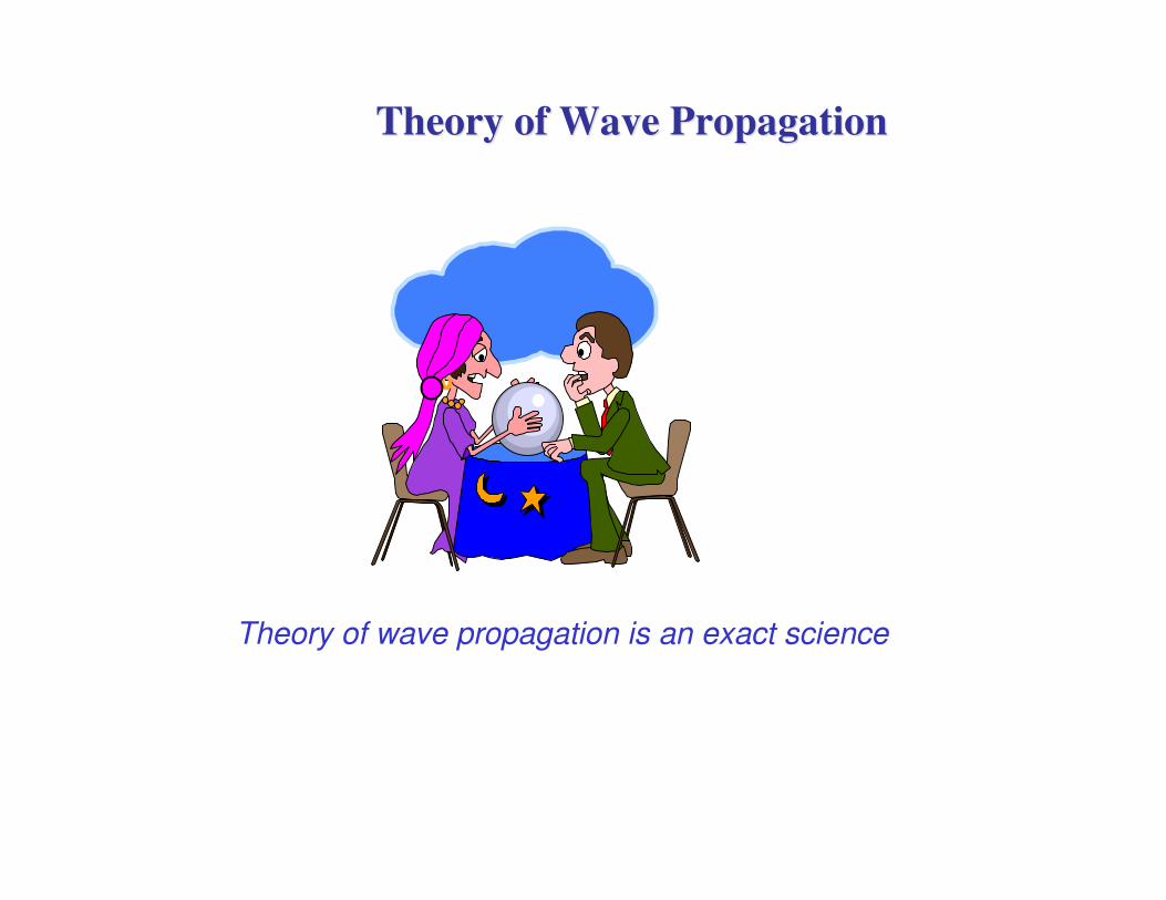
DiversityDiversity
Time diversity
Frequency diversity
Space diversity
Polarization diversity
Multi-path diversity
coding, interleaving
frequency hopping
multiple antennas
Dual-polarized antennas
equalizer
t
f

Benefit From DiversityBenefit From Diversity
Diversity gain depends on environment
Is there coverage improvement by diversity ?antenna diversity
5dB more signal strength
more path loss acceptable in link budget
higher coverage range
R
R(div) ~ 1,3 R A 1.7 A 70% more coverage per cell needs less cells in total
The above case can be satisfied only under Ideal condition. That is environment is infinitely large and flat

InterferenceInterference
we are HERE
2.1. Radio Wave Propagation
2.2. Propagation Models
2.3. Antenna Systems
2.4. Diversity Techniques
2.5. Interference
2.6. Interference Reduction
2.7. Link Budget Calculation

InterferenceInterference
Signal quality =
sum of all expected signals carrier (C )
sum of all unexpected signal interference ( I )=
• GSM specification : C / I >= 9 dB
expected signal atmospheric
noise
other signals

Effects of InterferenceEffects of Interference
Affects signal quality
Causes bit errors
repairable errors : channel coding, error correction
irreducible errors : phase distortions, random FM
Interference situation isnon- reciprocal uplink If. =/= downlink If.
unsymmetrical different situation at MS and BS
Concept C/I

Signal Quality in GSMSignal Quality in GSM
RX Quality (RXQUAL parameter)
RXQUAL classes 0 ... 7bit error rate before all decoding/ corrections
RXQUAL Mean BER BER range
class (%) from... to
0 0,14 < 0,2%
1 0,28 0,2 ... 0,4 %
2 0,57 0,4 ... 0,8 %
3 1,13 0,8 ... 1,6 %
4 2,26 1,6 ... 3,2 %
5 4,53 3,2 ... 6,4 %
6 9,05 6,4 ... 12,8 %
7 18,1 > 12,8 %
usable signal
unusable
signal
good
acceptable

Interference sourcesInterference sources
Multi-path components (long echoes)
Frequencies reusing
External interferences
• Network performance shall be interference-limited rather than coverage- limited
Push interference limits
as far as possible

Methods for reducing InterferenceMethods for reducing Interference
Frequency planning
Suitable site locations
Antenna (down-)tilting
good location
bad location

Methods for reducing InterferenceMethods for reducing Interference
Frequency hoppinga diversity technique, interference reduction as a side-effect
frequency diversity ==> less fading loss
de-coding gain
interference averaging
Quality based power control
evaluate signal level AND quality
DTXsilent transmitter in speech pauses
Adaptive antennasfollow the user
concentrate signal energy to certain directions
Adaptive channel allocationalways assign best available frequency during call-setup

Frequency HoppingFrequency Hopping
Diversity techniquefrequency diversity can reduce fast fading effects
useful for static or slow-moving mobiles
Cyclic base-band hoppingBS hops cyclic between its allocated frequencies (min. =3 TRX)
RF hoppingeither cyclic or random hopping
needs wideband combiner
can use any frequency included in the Hopping list (not on 1st TRX)
Frequency diversity for static mobilesfeature: interference averaging

Power ControlPower Control
Save battery life-time
Minimize interference
GSM : 15 steps and 2 dB for each
Use power control in both uplink & downlinklevel or quality-driven
time
signal
level target level
e.g. -85 dm
Power control not allowedon BCCH carrier

DTXDTX
DTX: discontinuous transmissionswitch transmitter off in speech pauses and silence periods
both sides transmit only silence updates (SID frames)
comfort noise generated by transcoder
VAD: voice activity detectiontranscoder function
Transcoder is informed on use of DTX/ VAD (in call
setup)
Battery saving and
Interface Reducing
Battery saving and
Interface Reducing

The Mobile Radio LinkThe Mobile Radio Link
we are HERE
2.1. Radio Wave Propagation
2.2. Propagation Models
2.3. Antenna Systems
2.4. Diversity Techniques
2.5. Interference
2.6. Interference Reduction
2.7. Link Budget Calculation

Link BudgetLink Budget
Why we need a link budget?
Which will decide the coverage range ?
The coverage range is limited by the weaker one (up or down link)
Two-way communication neededlink usually limited by mobile power
Desired result: downlink = uplink
Link budget must
be balanced

Network PlanningNetwork Planning
we are HERE 3.1. Cellular Planning Principles
3.2. Network Topologies
3.3. Traffic Estimation
3.4. Coverage Planning
3.5. Frequency Planning
3.6. Site Selection
3.7. Transmission Planning

Network Planning PrincipleNetwork Planning Principle
marketing
business plan
traffic assumptions
initial NWdimensioning
freq. & inter-ference plan
transmissionplan
final NW topology
parameter planning
coverage plan

Scope of Network PlanningScope of Network Planning
Network planning teamdata acquisition
site survey
field measurement evaluation
CW design and analysis
transmission planning
• Network design
• number and configuration of BS
• antenna systems specifications
• BSS topology
• dimensioning of transmission lines
• frequency plan
• network evolution strategy
• Network performance
• grade of service (blocking)
• outage calculations
• interference probabilities
• quality observation
• Operator’s requirements
• subscriber forecasts
• coverage requirements
• quality of service
• recommended sites
• External information sources
• terrain & morphological data
• population data
• bandwidth available
• frequency co-ordination constraints

Input DataInput Data
Mapsmain cities
important roads
location of mountain ranges
inhabited area
shore lines
Local knowledgecity skylines
typical architecture
structure of city

Demographic DataDemographic Data
Statistical yearbooklargest towns, cities
population distribution
where are expected customers?
Local knowledgepopulation migration routes
traffic volumes
subscriber concentration points
300 000 pop.
400 000 pop.
250 000 pop.

Network ConfigurationNetwork Configuration
Estimate number of BS neededVERY rough initial assumption :
total operator’s bandwidth
planned freq. re-use rate
number of BS needed for traffic reasons
Evaluate achievable cell sizes=f (topography, requirements, signal levels, environment, ...)
number of BS needed for coverage reasons
Normally: BS coverage >> BS traffic
==> problem with finance people
= average number of TRX allowed per cell
Finances Marketing
Planning

Network PlanningNetwork Planning
we are HERE
3.1. Cellular Planning Principles
3.2. Network Topologies
3.3. Traffic Estimation
3.4. Coverage Planning
3.5. Frequency Planning
3.6. Site Selection
3.7. Transmission Planning

Cell HierarchiesCell Hierarchies
Umbrella Cell/Macro cell
Micro cell
Pico cell
Satellite Cell

Macro Cell NetworkMacro Cell Network
Cost-effective solution
Suitable for covering large areaslarge cell ranges
high antenna positions
Cell ranges 2 ..20km
(depends on geography!)
Used with low traffic volumestypically rural areas
road coverage
Commonly use omnidirectional antennasuse beamed antenna for road coverage
2..20 km
Optimization for coverage

Micro Cell NetworkMicro Cell Network
Capacity oriented networkadditional capacity by multiple cell coverage
Suitable for areas with high traffic
Mostly used with beamed cellsmost cost-efficient solution
best usage of available cell sites
Typical applicationsmedium towns
suburbs
Typical coverage range: 0,5 .. 2km
Optimization for capacity
0,5 .. 2km

Cell coverage rangeCell coverage range
Achievable cell coverage range depend on
frequency band (450, 900, 1800 MHz)
surroundings, environment
link budget figures
antenna types
antenna positioning
minimum required signal levels

Hexagons and CellsHexagons and Cells
Three hexagons Three cells

Network PlanningNetwork Planning
we are HERE
3.1. Cellular Planning Principles
3.2. Network Topologies
3.3. Traffic Estimation
3.4. Coverage Planning
3.5. Frequency Planning
3.6. Site Selection
3.7. Transmission Planning

Traffic EstimationTraffic Estimation
Estimate number of subscribers over timelong-term predictions
numbers available from marketing people
Expected traffic load per subscriberdifferent subscriber segments
expected behavior of user segments
Particular habits of subscribers e.g. mainly heavy indoor usage
phoning while in traffic jams
Busy hour conditionstime of day
traffic patterns
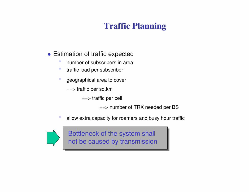
Traffic PlanningTraffic Planning
� Estimation of traffic expected
• number of subscribers in area
• traffic load per subscriber
• geographical area to cover
==> traffic per sq.km
==> traffic per cell
==> number of TRX needed per BS
• allow extra capacity for roamers and busy hour traffic
Bottleneck of the system shall
not be caused by transmission

Traffic PatternsTraffic Patterns
Traffic is not evenly spread across the day (or week)
Estimated traffic must be able to cope with peak
loadsBusy hour traffic is typically twice that of the average hour
0
10
20
30
40
50
60
70
80
90
100
0 2 4 6 8 10 12 14 16 18 20 22 24 hr
%
peak time
off-peak

Network PlanningNetwork Planning
we are HERE
3.1. Cellular Planning Principles
3.2. Network Topologies
3.3. Traffic Estimation
3.4. Coverage Planning
3.5. Frequency Planning
3.6. Site Selection
3.7. Transmission Planning

Coverage PlanningCoverage Planning
external inputs:(traffic, subs. forecast,
coverage requirements...)
Initial network dimensioning
TRXs, cells, sites
bandwidth needed
NW topology
nominal cell plansuggestions for
site locations
cell parameters
coverage achieved
coverage prediction
signal strength
multi-path propagation
coverage,
ok?
site inspection
site accepted ?
real cell planfield measurements
planning
criteria fulfilled?
N
N
N
create cell
data for
BSC
go to
frequency
planning

Coverage RequirementsCoverage Requirements
Roll-out phases & time schedules
Coverage level requirementsagree on min. levels for outdoor
coverage
Loss requirements
Indoor coverage areas
Mobile classes to plan for
Operator’s cell deployment
strategiesomni-cells in rural areas?
3-sector cells in urban areas?
phase 1CW launch
rolloutphase 2
rolloutphase 3

Coverage PlanningCoverage Planning
Loss
due to coverage gaps Pno_cov
due to interferences PIf
Total probable coverage area for a cell:
(1- Pno_cov) * (1- PIf)
Full coverage of an area can never be guaranteed !
common values: 90 .. 95% probability
(time and location probabilities)
Network planningNetwork planning
we are HERE
3.1. Cellular Planning Principles
3.2. Network Topologies
3.3. Dimensioning
3.4. Coverage Planning
3.5. Frequency Planning
3.6. Site Selection
3.7. Transmission Planning

Frequency PlanningFrequency Planning
� Why we reuse the frequency?
8 MHz = 40 channels * 8 timeslots = 320 users==> max. 320 simultaneous calls!!!
� Limited bandwidth
==> re-use frequencies as often as possible
� Interferences are unavoidable
==> minimize total interferences in network
� Allocate frequency combination that creates least overall interference
conditions in the network
� Use calculated propagation predictions for frequency allocations

Frequency Planning(1)Frequency Planning(1)
Target: find solution with minimum interferences in total
network
Traditional methodhexagonal cell patterns
regular grid
cluster sizes
frequency re-use distance
D = R *sqrt(3*cluster-size)
R
D
Do not use this ancient concept!

Frequency Planning(2)Frequency Planning(2)
Frequency planning always consider the worst
caseactual situation is less severe
power control, actual traffic and distribution of MS improve situation
Average frequency re-use rate as a criteria for
good allocation scheme:
practicallimits
safe, butuneconomical
physicallimit
0 10 20

Frequency Re-UseFrequency Re-Use
Re-use frequencies as often as
possibleincreases network capacity
but maybe cause some interferences
Do not usehexagon cell patterns
systematic frequency allocation
Butinterference matrix calculation
calibrated propagation models
minimize total interference in network
R
D
f2
f3
f4f5
f6
f7
f3
f4f5
f6
f2
f3
f4f5
f6f2
f3
f4f5
f6
f7
f2
f3
f4f5
f7
f2
f3
f4f5
f2
f3
f4f5
f6
f7

Multiple Re-use RatesMultiple Re-use Rates
Frequency re-use ratemeasure for effectiveness of frequency plan
trade-off : effectiveness interferences
Interactions (iteration loops) with coverage
planning
Multiple re-use rates increase effectiveness of freq.
plancompromise between safe, interference free planning and effective resource
usage
1 3 6 9 12 15 18 21
safe planning
(BCCH layer)normal planning
(TCH macro layer)
tight re-use planning
(tight layer)
same frequency
in every cell
(spread spectrum)

Multiple Re-use RatesMultiple Re-use Rates
Capacity increase with multiple re-use rates:e.g. network with 300 cells
bandwidth : 8 MHz (40 radio channels)
Single re-use: =12
==> NW capacity = 40/12 * 300 = 1000 TRX
Multiple re-use:BCCH layer: re-use =14, (14 freq.)
normal TCH: re-use =10, (20 freq.)
tight TCH layer: re-use = 6, (6 freq.)
==> NW cap. = (1 +2 +1)* 300 = 1200 TRX
cap NBW
re use
i
i
.=−
∑

Frequency Co-ordinationFrequency Co-ordination
Regulations for international boundaries25 dBµµµµV/m at borderline
10 dBµµµµV/m at 15km distance from border
Set of preferential and reserved frequencies must
be mutually agreed between operators
A
B
C
15km
international
borderline

Network PlanningNetwork Planning
we are HERE
3.1. Cellular Planning Principles
3.2. Network Topologies
3.3. Dimensioning
3.4. Coverage Planning
3.5. Frequency Planning
3.6. Site Selection
3.7. Transmission Planning

Site locationsSite locations
Cells performance has a close relationship with site location
Sites are expensive
Sites are long-term investments
Site acquisition is a slow process
Hundreds of sites needed per network
Base station site is a valuablelong-term asset for the operator

Bad Site LocationBad Site Location
Avoid hill-top locations for BS sitesuncontrolled interferences
interleaved coverage
awkward HO behaviors
but: good location for microwave links!
wanted cell
boundary
uncontrolled, strong
interferences
interleaved coverage areas:
weak own signal, strong foreign signal

Good Site LocationGood Site Location
•Prefer sites off the hill-tops• use hills to separate cells
• contiguous coverage area
• needs only low antenna heights if sites are slightly elevated above valley bottom
wanted cell
boundary

Site Selection CriteriaSite Selection Criteria
Radio criteria
good view in main beam
direction
no surrounding high
obstacles
good visibility of terrain
room for antenna mounting
LOS to next microwave site
short cabling distances
�Non-radio criteria
� space for equipment
� availability of leased lines or microwave link
� power supply
� access restrictions
� house owner
� rental costs

Site Acquisition ProcessSite Acquisition Process
radio planner
fixed networkplanner
measurementteams
architect
network operator
site hunter
site owner

Site InformationSite Information
Questionnaire sheet
collect all necessary information about site details
site coordinates, height above sea level, exact address
house owner
type of building
building materials (photo)
possible antenna heights
360deg photo (clearance view)
neighbourhood, surrounding environment
drawing sketch of rooftop
antenna mounting conditions
access possibilities (truck, road, roof)
BS location, approx. feeder lengths
Network planningNetwork planning
we are HERE
3.1. Cellular Planning Principles
3.2. Network Topologies
3.3. Dimensioning
3.4. Coverage Planning
3.5. Frequency Planning
3.6. Site Selection
3.7. Transmission Planning

Transmission PlanningTransmission Planning
Cost for transmission lines account for a great
portion of NW operational costs per year
==> design for minimum overall costs !
Fixed part design
MSC
BSC Hub
BTS
BSS
BTS
BTS
BTS
Radio part design
BTS
BSS
BTS
BTS
BTS

Transmission ConceptTransmission Concept
Transmission media
Transmission techniques
Transmission methods
Fiber
Coaxial cable
Copper cable
Microwave radioTerrestrial/satellite
PDH SDH
PCM
ISDN ATM
Tra
nsm
issio
n e
qu
ipm
en
tHDSL
CATV

Microwave LinksMicrowave Links
High capacity transmission links
Operating frequencies: 7 .. 38 GHz band
• Contra
� needs extra frequencies
� weather dependant link quality (rainfall)
� not always available at ideal sites (LOS path)
� long distance hops are problematic
• Pro
� low operating costs
� easy to install
� flexible
� quick & reliable solution
Terminalstation A
Terminalstation B
Repeaterstation
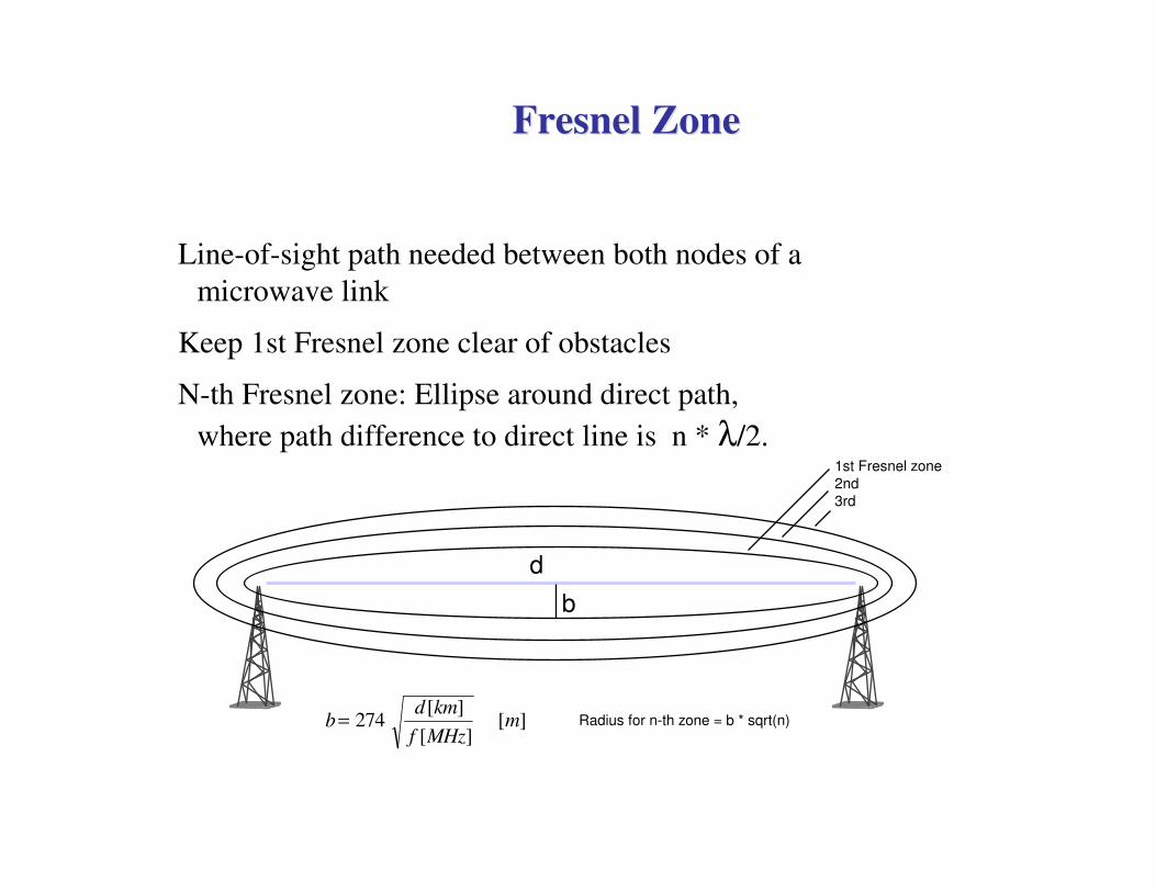
Fresnel ZoneFresnel Zone
Line-of-sight path needed between both nodes of a
microwave link
Keep 1st Fresnel zone clear of obstacles
N-th Fresnel zone: Ellipse around direct path,
where path difference to direct line is n * λ/2.
d
b
1st Fresnel zone
2nd
3rd
Radius for n-th zone = b * sqrt(n)bd km
f MHzm= 274
[ ]
[ ][ ]
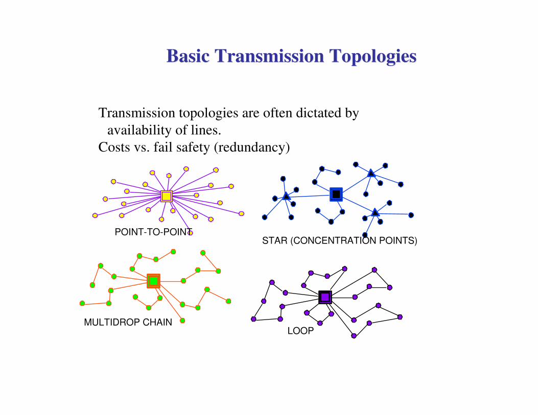
Basic Transmission TopologiesBasic Transmission Topologies
Transmission topologies are often dictated by
availability of lines.
Costs vs. fail safety (redundancy)
POINT-TO-POINT
MULTIDROP CHAINLOOP
STAR (CONCENTRATION POINTS)

Network topologyNetwork topology
Prefer centralized or decentralized NW architecture
2 small BSC plus
cheap transmission
1 large BSC plus
expensive
transmission
MSC
BTS
BSC
BTS
BTS
BTS
BSC/ MSC
BTS
BTS
BTS
BTS

Cross-ConnectsCross-Connects
Transmission equipment to branch data streams
between different link sets
Non-blocking stageeach input stream is routed to an output stream
Tasksswitching between link sets
switching between timeslots of a PCM trunk
dropping & inserting timeslots

Advanced Network Planning ItemsAdvanced Network Planning Items
we are HERE 4.1. Network evolution
4.2. Indoor coverage
4.3. Tunnel coverage
4.4. Parameters
4.5. Network Optimizing

Cell Size EvolutionCell Size Evolution
LARGE CELLS
5-50 km
Early 80's
SMALL CELLS
1-5 km
Mid-end 80's
MICROCELLS
100 m - 1 km
Mid 90
PICOCELLS
10-100m
MACRO CELLS
's 's
LAYERED NETWORK
Smaller Cells Bring Higher Capacities but ...Smaller Cells Bring Higher Capacities but ...
Logistics of planning and implementation
=> bottleneck to small cell deployment
Small cells must be integrated into network & managed by
advanced BSS

Layered NetworkLayered Network
Micro cell
Macro cell
Micro cell
Micro cell

Network Capacity evolutionNetwork Capacity evolution
Measure for network spectral efficiency:Erl/ (MHz * sq.km)
A function ofbandwidth
frequency efficiency of technology
frequency re-use
cell sizes
trunking gains
Frq. hoppingFrq. hopping
DTXDTX
Directed
Retry
Directed
Retry
Power
Control
Power
Control
Half-rate
code
Half-rate
code
Load
distribution
Load
distribution
Traffic
reason HO
Traffic
reason HO
multiple cell
coverage
multiple cell
coverage

Advanced Network Planning ItemsAdvanced Network Planning Items
4.1. Network evolution
4.2. Indoor coverage
4.3. Tunnel coverage
4.4. Parameters
We are HERE

Why IndoorsWhy Indoors
• Cellular competition moves indoors
• Subscribers expect continuous coverage and quality
• Outdoor cells do not provide sufficient coverage indoors
INDOOR SOLUTION
Good Quality!

BenefitsBenefits
Low Transmitting Powers (BTS/MS)
DedicatedIndoor Solution
Good Quality
Safety
MS Battery Life
Office Equipment
Less Interference
Continuous Coverage
Subscriber value
Continuous Service

Building LossesBuilding Losses
Signal levels in buildings are estimated by
applying a building penetration loss margin
Big differences between rooms with window and
deep indoor(10 ..15 dB)
Pref = 0 dB
Pindoor = -3 ...-15 dB
Pindoor = -7 ...-18 dB
-15 ...-25 dB no coverage
rear side :
-18 ...-30 dB
signal level increases with floor
number :~1,5 dB/floor (for 1st
..10th floor)

Building Penetration LossBuilding Penetration Loss
Signal losses for building penetration vary greatly
with building materials used, e.g.:
mean value sigmareinforced concrete wall, windows 17 dB 9concrete wall, no windows 30 dB 9concrete wall within building 10 dB 7brick wall 9 dB 6armed glass 8 dB 6wood or plaster wall 6 dB 6window glass 2 dB 6
No major differences for 900 or 1800 MHz
Total building loss =add median values
superimpose standard deviations
add (lognormal) margin for higher probabilities

In-Building Path LossIn-Building Path Loss
Simple path loss model for in-building
environment
outdoor losses: Okumura‘s formula
Lout = 42,6 + 20 log( f ) + 26 .. 35 log( d )
wall losses:
Lwall = f(material; angle)
indoor losses: linear model for picocells
Lin = L0 + αααα d
building type losses application example
old house 0,7 dB/m (urban residential)
commercial type 0,5 dB/m (modern offices)
open room, atrium 0,2 dB/m (museum, train station)
Lout
Lwall
Lin

Indoor Coverage SolutionsIndoor Coverage Solutions
Small BTSmini BTS
PrimeSite
Repeatersactive, passive
optical
Antennasdistributed antennas
radiating cable
Signal distributionpower splitters
optical fiber
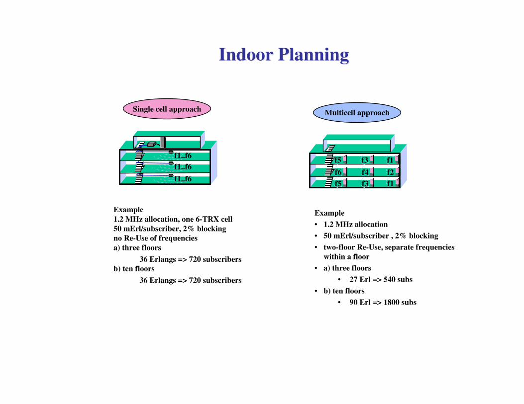
Indoor PlanningIndoor Planning
Example
• 1.2 MHz allocation
• 50 mErl/subscriber , 2% blocking
• two-floor Re-Use, separate frequencies
within a floor
• a) three floors
• 27 Erl => 540 subs
• b) ten floors
• 90 Erl => 1800 subs
Example
1.2 MHz allocation, one 6-TRX cell
50 mErl/subscriber, 2% blocking
no Re-Use of frequencies
a) three floors
36 Erlangs => 720 subscribers
b) ten floors
36 Erlangs => 720 subscribers
Single cell approachMulticell approach
t
f5
f6
f5
f1
f2
f1
f3
f4
f3f1..f6
f1..f6
f1..f6

Radiating cableRadiating cable
Coaxial cable with perforated leads
==> energy leak
Radiating losses 10 ..40 dB per 100m
coupling loss typ. 55 dB (at 1m ref. dist.)
Produce constant fieldstrengths along cable runs
Operate in wide frequency range
radiating losses become higher with frequency
Very large bending radii
disturbs field distribution
Formerly often used for tunnel coverage
VERY EXPENSIVE

Indoor Coverage ExamplesIndoor Coverage Examples
1:1
50m
50m
1:1
50m
50m
1:1
50m
50m
1:1
50m
50m
1:1
50m
50m
1:1
1:1:1
1:1
4th floor
3rd floor
2nd floor
1st floor
ground floor
With repeaterrelay outdoor signal into target building
needs donor cell; adds coverage, no capacity
With indoor BTS and distributed antennasheavy losses by power splitting and cabling
Outdoor Antenna
Gain: 18 dBi
Indoor Antenna
Gain: 9dBi
Target Indoor Coverage Building
7/8'' Cable Loss: 4dB / 50mCable length : 25m
-50 dBm
4th Floor
3rd Floor
1st Floor
Ground Floor
2nd Floor
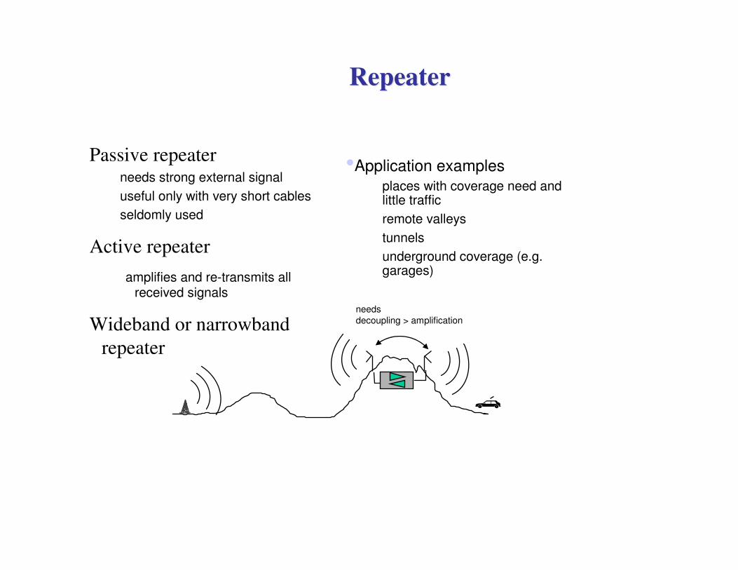
RepeaterRepeater
Passive repeaterneeds strong external signal
useful only with very short cables
seldomly used
Active repeater
amplifies and re-transmits all received signals
Wideband or narrowband
repeater
•Application examples
places with coverage need and little traffic
remote valleys
tunnels
underground coverage (e.g. garages)
needs
decoupling > amplification

The Light-bulb PrinciplesThe Light-bulb Principles
several smaller sites provide more indoor coverage area than a single large site
... is better than ...

Newspaper PrinciplesNewspaper Principles
Indoor coverage may be expected in locations where there is no enough daylight to comfortably read a newspaper without artificial illumination
• Where NOT? e.g.
hotel lobby
elevator
hallways
• Where? e.g.
rooms with window
near a window
atrium-style places
• The newspaper-principle

Wave Propagation in TunnelsWave Propagation in Tunnels
Tunnels are very friendly environment
for radio wave propagation
Tunnels are very friendly environment
for radio wave propagation
Ideal antenna position: center of cross-section
Distance to walls: min. 2 λ
Tunnel cross-section shape unimportant, if > 10 λ
Time dispersion decreases with distance ==>constant
Mount antenna ~50..100m before tunnel entrance
Good signal coupling between successive tunnels

Tunnel Cross-SectionTunnel Cross-Section
Filling factor determines propagation conditions
Typical ranges for filling factorsroad tunnels: 10%
Metro: 60..90%
filling factor =----------

Advanced Network Planning ItemsAdvanced Network Planning Items
we are HERE
4.1. Network evolution
4.2. Indoor coverage
4.3. Tunnel coverage
4.4. Parameters

BSS ParametersBSS Parameters
Relevant BSS parameter for NW planning
frequency allocation plan
logical radio interface configuration
transmit power
definition of neighboring cells
definition of location areas
handover parameters
power control parameters
cell selection parameters
radio link time-out settings
topology of BSC- BTS network

Handover TypesHandover Types
Intra-cell same cell, different carrier or
timeslot
Inter-cell different cells (normal case)
Inter-BSC different BSC
Inter-MSC different MSC areas
Inter-PLMN (technically feasible, not supported)
Intra-cell
Inte-rcell
inter-BSC

Handover CriteriaHandover Criteria
1. Interference, UL and DL2. Bad C/I ratio3. Uplink Quality 4. Downlink Quality 5. Uplink Level 6. Downlink Level 7. Distance8. Rapid Field Drop
�9. MS Speed
�10. Better Cell, i.e. periodic check (Power Budget)
�11. Good C/I ratio
�12. PC: Lower quality/level thresholds (DL/UL)
�13. PC: Upper quality/level thresholds (DL/UL)
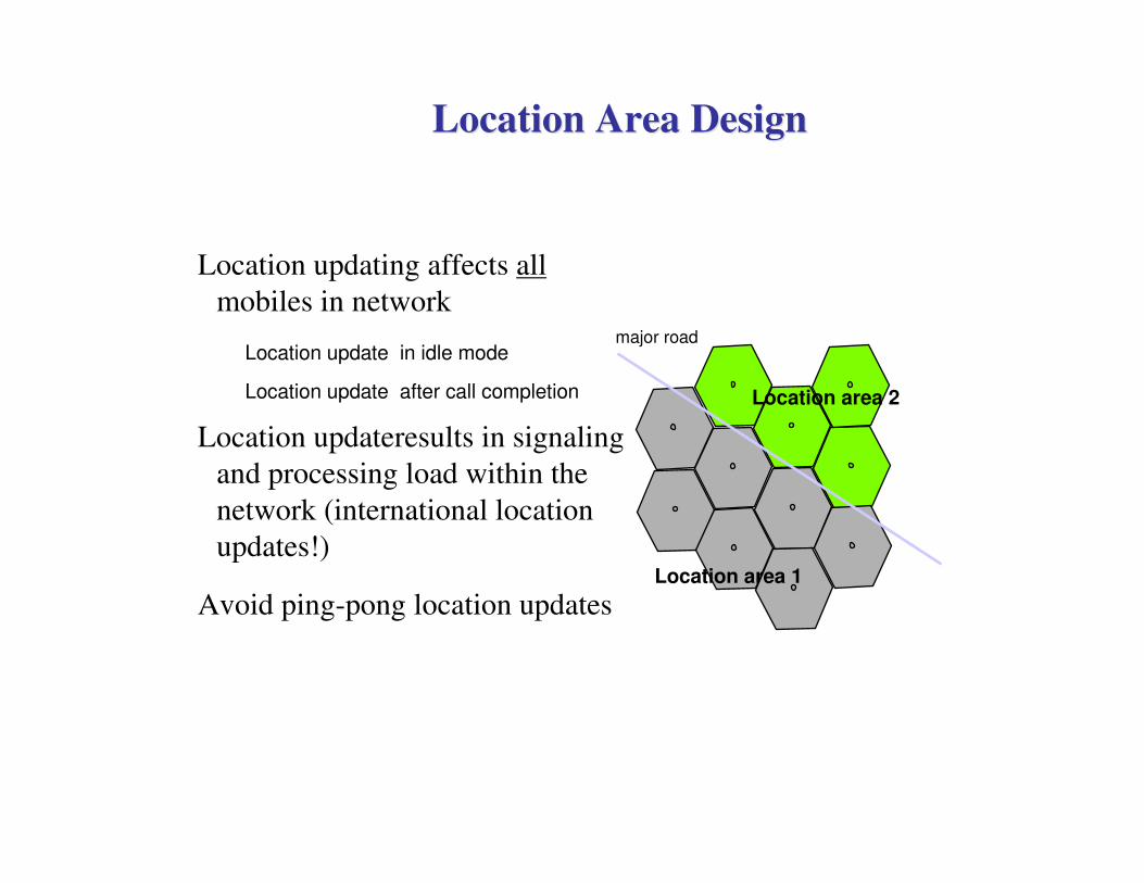
Location Area DesignLocation Area Design
Location updating affects all
mobiles in network
Location update in idle mode
Location update after call completion
Location updateresults in signaling
and processing load within the
network (international location
updates!)
Avoid ping-pong location updatesLocation area 1
Location area 2
major road
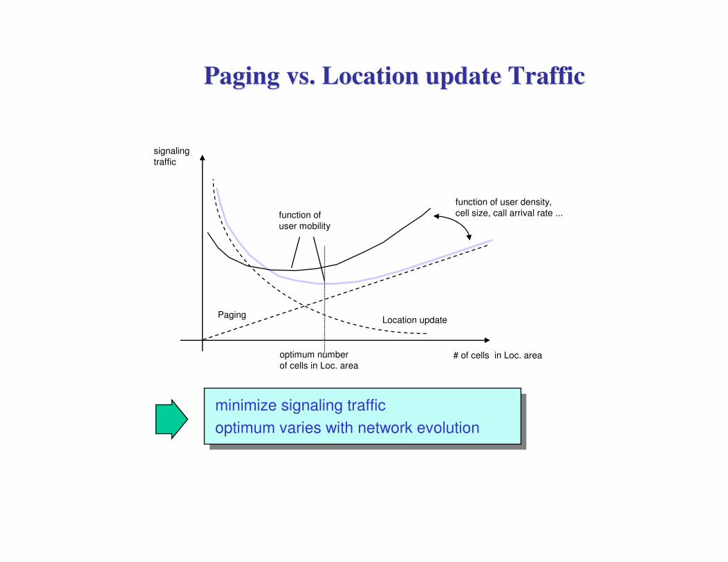
Paging vs. Location update TrafficPaging vs. Location update Traffic
PagingLocation update
# of cells in Loc. area
signaling
traffic
optimum number
of cells in Loc. area
function of user density,
cell size, call arrival rate ...function of
user mobility
minimize signaling traffic
optimum varies with network evolution

Thank you