4.7 Statistical Modeling of Photographic Images

Eero P. SimoncelliNew York University

January 18, 2005

To appear in: Handbook of Video and Image Processing, 2nd editioned. Alan Bovik, c©Academic Press, 2005.

The set of all possible visual images is huge, but not all ofthese are equally likely to be encountered by an imagingdevice such as the eye. Knowledge of this nonuniformprobability on the image space is known to be exploitedby biological visual systems, and can be used to advan-tage in the majority of applications in image processingand machine vision. For example, loosely speaking, whenone observes a visual image that has been corrupted bysome sort of noise, the process of estimating the originalsource image may be viewed as one of looking for thehighest-probability image that is “close to” the noisy ob-servation. The problem of compression essentially boilsdown to using a larger proportion of the available bits toencode those regions of the image space that are morelikely. And problems such as resolution enhancementor image synthesis involve selecting (sampling) a high-probability image from the distribution, perhaps subjectto some set of constraints. Precise developments of suchapplications can be found in many chapters throughoutthis book.

In order to develop a probability model for visual images,we first must decide which images to model. In a prac-tical sense, this means we must (a) decide on imagingconditions, such as the field of view, resolution, sensor orpostprocessing nonlinearities, etc, (b) decide what kind ofscenes, under what kind of lighting, are to be captured inthe images. It may seem odd, if one has not encounteredsuch models, to imagine that all images are drawn froma single universal probability urn. In particular, the fea-tures and properties in any given image are often special-ized. For example, outdoor nature scenes contain struc-tures that are quite different from city streets, which inturn are nothing like human faces. There are two meansby which this dilemma is resolved. First, the statisticalproperties that we will examine are basic enough thatthey are relevant for essentially all visual scenes. Second,we will use parametric models, in which a set of hyperpa-

rameters (possibly random variables themselves) governthe detailed behavior of the model, and thus allow a cer-tain degree of adaptability of the model to different typesof source material.

How does one build and test a probability model for im-ages? Many approaches have been developed, but in thischapter, we’ll describe an empirically-driven methodol-ogy, based on the study of discretized (pixelated) im-ages. Currently available digital cameras record such im-ages, typically containing millions of pixels. Naively, onecould imagine examining a large set of such images to tryto determine how they are distributed. But a moment’sthought leads one to realize the hopelessness of the en-deavor. The amount of data needed to estimate a proba-bility distribution from samples grows as KD, where D isthe dimensionality of the space (in this case, the numberof pixels). This is known as the “curse of dimensionality”.

Thus, in order to make progress on image modeling,it is essential to reduce the dimensionality of the space.Two types of simplifying assumption can help in this re-gard. The first, known as a Markov assumption, is thatthe probability density of a pixel, when conditioned ona set of pixels in a small spatial neighborhood, is inde-pendent of the pixels outside of the neighborhood. Asecond type of simplification comes from imposing cer-tain symmetries or invariances on the probability struc-ture. The most common of these is that of translation-invariance (i.e., sometimes called homogeneity, or strict-sense stationarity): the distribution of pixels in a neigh-borhood does not depend on the absolute location of thatneighborhood within the image. This seems intuitivelysensible, given that a lateral or vertical translation of thecamera leads approximately to a translation of the imageintensities across the pixel array. Note that translation-invariance is not well defined at the boundaries, and as isoften the case in image processing, these locations mustusually be handled specially.

Another common assumption is scale-invariance: resiz-ing the image does not alter the probability structure.This may also be loosely justified by noting that adjust-ing the focal length (zoom) of a camera lens approximates(apart from perspective distortions) image resizing. Aswith translation-invariance, scale-invariance will clearlyfail to hold at certain “boundaries”. Specifically, scale-invariance must fail for discretized images at fine scalesapproaching the size of the pixels. And similarly, it mustalso fail for finite size images at coarse scales approachingthe size of the entire image.

With these sort of simplifying structural assumptions inplace, we can return to the problem of developing a prob-ability model. In recent years, researchers from imageprocessing, computer vision, physics, applied math andstatistics have proposed a wide variety of different typesof model. In this chapter, I’ll review some basic statisticalproperties of photographic images, as observed empiri-cally, and describe several models that have been devel-oped to incorporate these properties. I’ll give some indi-cation of how these models have been validated by exam-ining how well they fit the data, but the true test usuallycomes when one uses the model to solve an image pro-cessing problem (such as compression or denoising). Al-though this is somewhat beyond the scope of this chapter,I’ll show some simple denoising examples to give an in-dication of how much performance gain one can obtainby using a better statistical model. In order to keep thediscussion focused, I’ll limit the discussion to discretizedgrayscale photographic images. Many of the principles areeasily extended to color photographs [8, 43], or temporalimage sequences (movies) [15], as well as more special-ized image classes such as portraits, landscapes, or tex-tures. In addition, the general approach may also be ap-plied to non-visual imaging devices, such as medical im-ages, infrared images, radar and other types of range im-age, or astronomical images.

1 The Gaussian Model

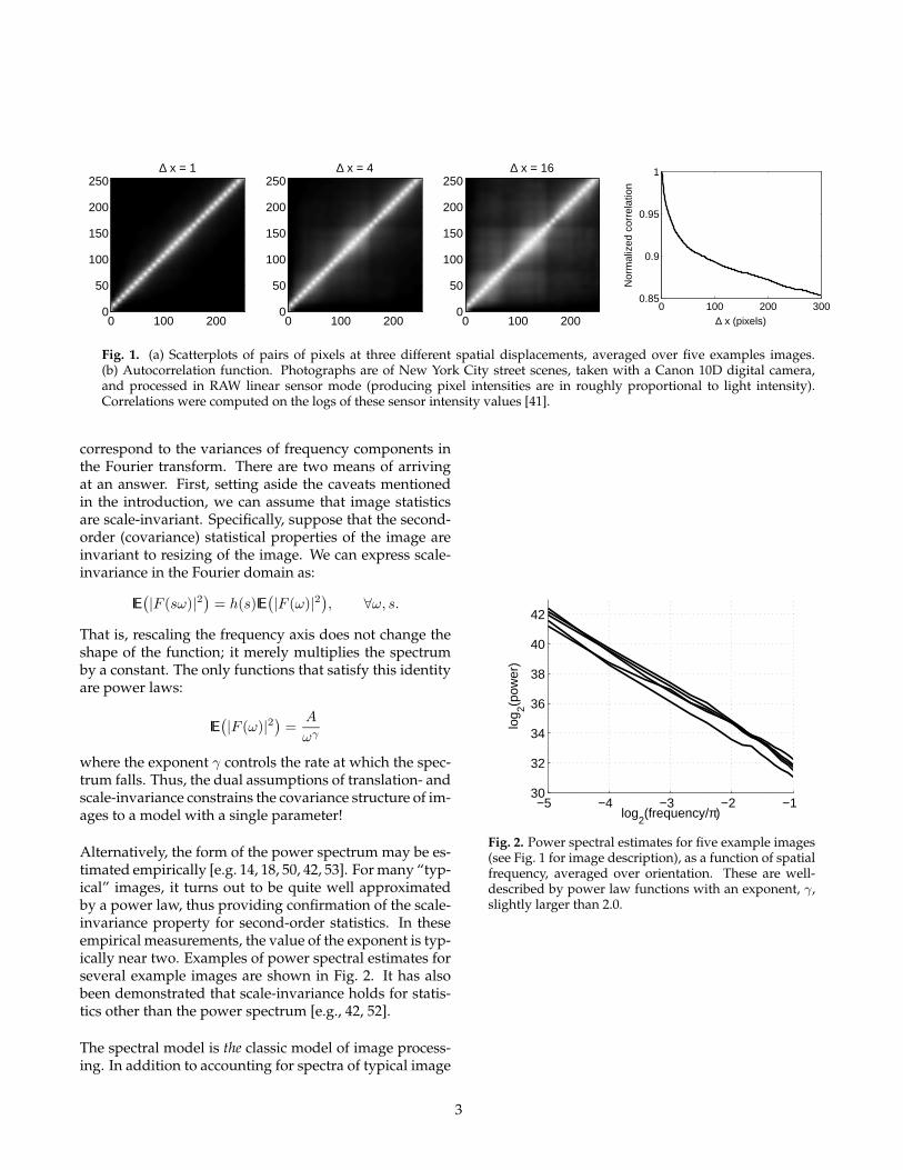
The classical model of image statistics was developed bytelevision engineers in the 1950s (see [41] for a review),who were interested in optimal signal representation andtransmission. The most basic motivation for these mod-els comes from the observation that pixels at nearby loca-tions tend to have similar intensity values. This is easilyconfirmed by measurements like those shown in Fig. 1(a).Each scatterplot shows values of a pair of pixels with a

given relative spatial displacement. Implicit in these mea-surements is the assumption of homogeneity mentionedin the introduction: the distributions are assumed to beindependent of the absolute location within the image.And although the pixels were taken from a single photo-graphic image (in this case, a New York City street scene),they are nevertheless representative of what one sees inmost visual images.

The most striking behavior observed in the plots is thatthe pixel values are highly correlated: when one is large,the other tends to also be large. But this correlation fallswith the distance between pixels. This behavior is sum-marized in Fig. 1(b), which shows the image autocorrela-tion (pixel correlation as a function of separation).

The correlation statistics of Fig. 1 place a strong constrainton the structure of images, but they do not provide afull probability model. Specifically, there are many prob-ability densities that would share the same correlation(or equivalently, covariance) structure. How should wechoose a model from amongst this set? One natural crite-rion is to select a density that has maximal entropy, sub-ject to the covariance constraint [25]. Solving for this den-sity turns out to be relatively straighforward, and the re-sult is a multi-dimensional Gaussian:

P(~x) ∝ exp(−~xTCx

−1~x/2), (1)

where ~x is a vector containing all of the image pixels (as-sumed, for notational simplicity, to be zero-mean) andCx ≡ IE~x~xT is the covariance matrix.

Gaussian densities are more succinctly described bytransforming to a coordinate system in which the covari-ance matrix is diagonal. This is easily achieved usingstandard linear algebra techniques:

~y = ET ~x,

where E is an orthogonal matrix containing the eigenvec-tors of Cx, such that

Cx = EDET , =⇒ ETCxE = D, (2)

with D a diagonal matrix containing the associated eigen-values. When the probability distribution on ~x is station-ary (assuming periodic handling of boundaries), the co-variance matrix, Cx, will be circulant. In this special case,the Fourier transform is known in advance to be a diag-onalizing transformation matrix E, and is guaranteed tosatisfy the relationship of Eq. (2).

In order to complete the Gaussian image model, we needonly specify the entries of the diagonal matrix D, which

2

∆ x = 1

0 100 2000

50

100

150

200

250∆ x = 4

0 100 2000

50

100

150

200

250∆ x = 16

0 100 2000

50

100

150

200

250

0 100 200 3000.85

0.9

0.95

1

∆ x (pixels)

Nor

mal

ized

cor

rela

tion

Fig. 1. (a) Scatterplots of pairs of pixels at three different spatial displacements, averaged over five examples images.(b) Autocorrelation function. Photographs are of New York City street scenes, taken with a Canon 10D digital camera,and processed in RAW linear sensor mode (producing pixel intensities are in roughly proportional to light intensity).Correlations were computed on the logs of these sensor intensity values [41].

correspond to the variances of frequency components inthe Fourier transform. There are two means of arrivingat an answer. First, setting aside the caveats mentionedin the introduction, we can assume that image statisticsare scale-invariant. Specifically, suppose that the second-order (covariance) statistical properties of the image areinvariant to resizing of the image. We can express scale-invariance in the Fourier domain as:

IE(

|F (sω)|2)

= h(s)IE(

|F (ω)|2)

, ∀ω, s.

That is, rescaling the frequency axis does not change theshape of the function; it merely multiplies the spectrumby a constant. The only functions that satisfy this identityare power laws:

IE(

|F (ω)|2)

=A

ωγ

where the exponent γ controls the rate at which the spec-trum falls. Thus, the dual assumptions of translation- andscale-invariance constrains the covariance structure of im-ages to a model with a single parameter!

Alternatively, the form of the power spectrum may be es-timated empirically [e.g. 14, 18, 50, 42, 53]. For many “typ-ical” images, it turns out to be quite well approximatedby a power law, thus providing confirmation of the scale-invariance property for second-order statistics. In theseempirical measurements, the value of the exponent is typ-ically near two. Examples of power spectral estimates forseveral example images are shown in Fig. 2. It has alsobeen demonstrated that scale-invariance holds for statis-tics other than the power spectrum [e.g., 42, 52].

The spectral model is the classic model of image process-ing. In addition to accounting for spectra of typical image

−5 −4 −3 −2 −130

32

34

36

38

40

42

log2(frequency/π)

log 2(p

ower

)

Fig. 2. Power spectral estimates for five example images(see Fig. 1 for image description), as a function of spatialfrequency, averaged over orientation. These are well-described by power law functions with an exponent, γ,slightly larger than 2.0.

3

data, the simplicity of the Gaussian form leads to directsolutions for image compression and denoising that maybe found in essentially any textbook on image processing.As an example, consider the problem of removing addi-tive Gaussian white noise from an image, ~x. The degra-dation process is described by the conditional density ofthe observed (noisy) image, ~y, given the original (clean)image ~x:

P(~y|~x) ∝ exp(−||~y − ~x||2/2σ2

n)

where σ2

n is the variance of the noise. Using Bayes’ Rule,we can reverse the conditioning by multiplying by theprior probability density on ~x:

P(~x|~y) ∝ exp(−||~y − ~x||2/2σ2

n) · P(~x).

An estimate for ~x may now be obtained from this poste-rior density. One can, for example, choose the ~x that maxi-mizes the probability (the maximum a posteriori or MAP es-timate), or the mean of the density (the Bayes Least Squaresor BLS estimate). In the case of a Gaussian prior of Eq. 1,these two solutions are identical.

x(~y) = Cx(Cx + σ2

n)−1~y.

The solution is linear in the observed (noisy) image ~y.Finally, the solution may be rewritten in the Fourier do-main, where the scale-invariance of the power spectrummay be explicitly incorporated:

X(ω) =A/ωγ

A/ωγ + σ2n

· Y (ω),

where X(ω) and Y (ω) are the Fourier transforms of x(~y)and ~y, respectively. Thus, the estimate may be computedby linearly rescaling each Fourier coefficient. In order toapply this denoising method, one must be given (or mustestimate) the parameters, A, γ and σn.

Despite the simplicity and tractability of the Gaussianmodel, it is easy to see that the model provides a ratherweak description. In particular, while the model stronglyconstrains the amplitudes of the Fourier coefficients, itplaces no constraint on their phases. When one random-izes the phases of an image, the appearance is completelydestroyed [37].

As a direct test, one can draw sample images from the dis-tribution by simply generating white noise in the Fourierdomain, weighting each sample appropriately by 1/ωγ ,and then inverting the transform to generate an image.An example is shown in Fig. 3. The fact that such an ex-periment invariably produces images of clouds impliesthat a covariance constraint is insufficient to capture thericher structure of features that are found in most real im-ages.

Fig. 3. Example image randomly drawn from the Gaus-sian spectral model, with γ = 2.0.

2 The Wavelet Marginal Model

For decades, the inadequacy of the Gaussian model wasapparent. But direct improvement, through introductionof constraints on the Fourier phases, turned out to bequite difficult. Relationships between phase componentsare not easily measured, in part because of the difficultyof working with joint statistics of circular variables, andin part because the dependencies between phases of dif-ferent frequencies do not seem to be well captured by amodel that is localized in frequency. A breakthrough oc-curred in the 1980s, when a number of authors began todescribe more direct indications of non-Gaussian behav-iors in images. Specifically, a multidimensional Gaussianstatistical model has the property that all conditional ormarginal densities must also be Gaussian. But these au-thors noted that histograms of bandpass-filtered naturalimages were highly non-Gaussian [9, 18, 13, 31, 58]. Thesemarginals tend to be much more sharply peaked at zero,with more extensive tails, when compared with a Gaus-sian of the same variance. As an example, Fig. 4 showshistograms of three images, filtered with a Gabor function(a Gaussian-windowed sinuosoidal grating). The intu-itive reason for this behavior is that images typically con-tain smooth regions, punctuated by localized “features”such as lines, edges or corners. The smooth regions leadto small filter responses that generate the sharp peak atzero, and the localized features produce large-amplituderesponses that generate the extensive tails.

This basic behavior holds for essentially any bandpass fil-ter, whether it is non-directional (center-surround), or ori-ented, but some filters lead to responses that are more

4

Wavelet coefficient value

log(

Pro

babi

lity)

p = 0.46∆H/H = 0.0031

Wavelet coefficient valuelo

g(P

roba

bilit

y)

p = 0.58∆H/H = 0.0011

Wavelet coefficient value

log(

Pro

babi

lity)

p = 0.48∆H/H = 0.0014

Wavelet coefficient value

log(

Pro

babi

lity)

p = 0.59∆H/H = 0.0012

Fig. 4. Log histograms of a single wavelet subband of four example images (see Fig. 1 for image description). For eachhistogram, tails are truncated so as to show 99.8% of the distribution. Also shown (dashed lines) are fitted model densitiescorresponding to equation (3). Text indicates the maximum-likelihood value of p used for the fitted model density, andthe relative entropy (Kullback-Leibler divergence) of the model and histogram, as a fraction of the total entropy of thehistogram.

non-Gaussian than others. By the mid 1990s, a numberof authors had developed methods of optimizing a ba-sis of filters in order to to maximize the non-Gaussianityof the responses [e.g., 36, 4]. Often these methods oper-ate by optimizing a higher-order statistic such as kurto-sis (the fourth moment divided by the squared variance).The resulting basis sets contain oriented filters of differentsizes with frequency bandwidths of roughly one octave.Figure 5 shows an example basis set, obtained by opti-mizing kurtosis of the marginal responses to an ensembleof 12 × 12 pixel blocks drawn from a large ensemble ofnatural images. In parallel with these statistical develop-ments, authors from a variety of communities were devel-oping multi-scale orthonormal bases for signal and imageanalysis, now generically known as “wavelets” (see chap-ter 4.2 in this volume). These provide a good approxima-tion to optimized bases such as that shown in Fig. 5.

Once we’ve transformed the image to a multi-scalewavelet representation, what statistical model can we useto characterize the the coefficients? The statistical moti-vation for the choice of basis came from the shape of themarginals, and thus it would seem natural to assume thatthe coefficients within a subband are independent andidentically distributed. With this assumption, the modelis completely determined by the marginal statistics of thecoefficients, which can be examined empirically as in theexamples of Fig. 4. For natural images, these histogramsare surprisingly well described by a two-parameter gen-eralized Gaussian (also known as a stretched, or generalizedexponential) distribution [e.g., 31, 47, 34]:

Pc(c; s, p) =exp(−|c/s|p)

Z(s, p), (3)

where the normalization constant is Z(s, p) = 2 spΓ( 1

p ).An exponent of p = 2 corresponds to a Gaussian den-sity, and p = 1 corresponds to the Laplacian density. In

Fig. 5. Example basis functions derived by optimizing amarginal kurtosis criterion [see 35].

5

general, smaller values of p lead to a density that is bothmore concentrated at zero and has more expansive tails.Each of the histograms in Fig. 4 is plotted with a dashedcurve corresponding to the best fitting instance of thisdensity function, with the parameters {s, p} estimated bymaximizing the likelihood of the data under the model.The density model fits the histograms remarkably well,as indicated numerically by the relative entropy measuresgiven below each plot. We have observed that values ofthe exponent p typically lie in the range [0.4, 0.8]. The fac-tor s varies monotonically with the scale of the basis func-tions, with correspondingly higher variance for coarser-scale components.

This wavelet marginal model is significantly more pow-erful than the classical Gaussian (spectral) model. Forexample, when applied to the problem of compression,the entropy of the distributions described above is signif-icantly less than that of a Gaussian with the same vari-ance, and this leads directly to gains in coding efficiency.In denoising, the use of this model as a prior density forimages yields to significant improvements over the Gaus-sian model [e.g., 48, 11, 2, 34, 47]. Consider again theproblem of removing additive Gaussian white noise froman image. If the wavelet transform is orthogonal, then thenoise remains white in the wavelet domain. The degra-dation process may be described in the wavelet domainas:

P(d|c) ∝ exp(−(d − c)2/2σ2

n)

where d is a wavelet coefficient of the observed (noisy)image, c is the corresponding wavelet coefficient of theoriginal (clean) image, and σ2

n is the variance of the noise.Again, using Bayes’ Rule, we can reverse the condition-ing:

P(c|d) ∝ exp(−(d − c)2/2σ2

n) · P(c),

where the prior on c is given by Eq. (3). The MAP and BLSsolutions cannot, in general, be written in closed form, butnumerical solutions are fairly easy to compute [48, 47].The resulting estimators are nonlinear “coring” functions,in which small-amplitude coefficients are suppressed andlarge-amplitude coefficients preserved. These estimatesshow substantial improvement over the linear estimatesassociated with the Gaussian model of the previous sec-tion (see examples in Fig. 10).

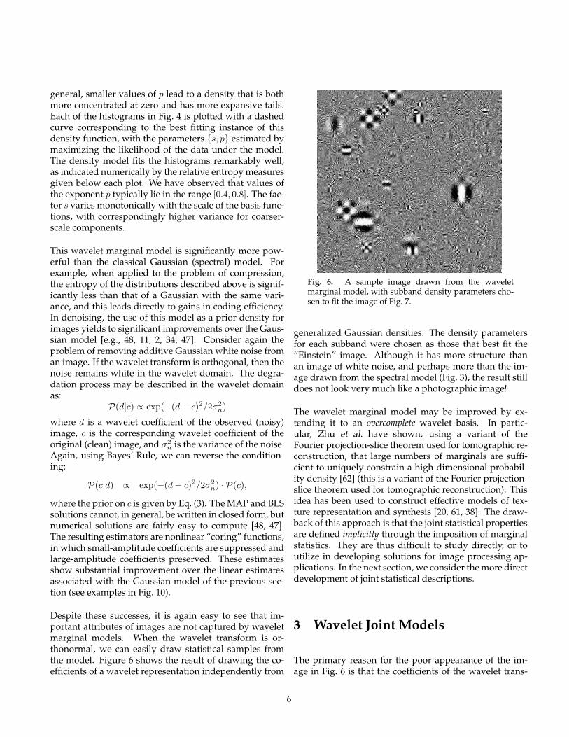
Despite these successes, it is again easy to see that im-portant attributes of images are not captured by waveletmarginal models. When the wavelet transform is or-thonormal, we can easily draw statistical samples fromthe model. Figure 6 shows the result of drawing the co-efficients of a wavelet representation independently from

Fig. 6. A sample image drawn from the waveletmarginal model, with subband density parameters cho-sen to fit the image of Fig. 7.

generalized Gaussian densities. The density parametersfor each subband were chosen as those that best fit the“Einstein” image. Although it has more structure thanan image of white noise, and perhaps more than the im-age drawn from the spectral model (Fig. 3), the result stilldoes not look very much like a photographic image!

The wavelet marginal model may be improved by ex-tending it to an overcomplete wavelet basis. In partic-ular, Zhu et al. have shown, using a variant of theFourier projection-slice theorem used for tomographic re-construction, that large numbers of marginals are suffi-cient to uniquely constrain a high-dimensional probabil-ity density [62] (this is a variant of the Fourier projection-slice theorem used for tomographic reconstruction). Thisidea has been used to construct effective models of tex-ture representation and synthesis [20, 61, 38]. The draw-back of this approach is that the joint statistical propertiesare defined implicitly through the imposition of marginalstatistics. They are thus difficult to study directly, or toutilize in developing solutions for image processing ap-plications. In the next section, we consider the more directdevelopment of joint statistical descriptions.

3 Wavelet Joint Models

The primary reason for the poor appearance of the im-age in Fig. 6 is that the coefficients of the wavelet trans-

6

Fig. 7. Amplitudes of multi-scale wavelet coefficients forthe “Einstein” image. Each subimage shows coefficientamplitudes of a subband obtained by convolution witha filter of a different scale and orientation, and subsam-pled by an appropriate factor. Coefficients that are spa-tially near each other within a band tend to have similaramplitudes. In addition, coefficients at different orienta-tions or scales but in nearby (relative) spatial positionstend to have similar amplitudes.

form are not independent. Empirically, the coefficientsof orthonormal wavelet decompositions of visual imagesare found to be moderately well decorrelated (i.e., theircovariance is zero). But this is only a statement abouttheir second-order dependence, and one can easily see thatthere are important higher-order dependencies. Figure 7shows the amplitudes (absolute values) of coefficients in afour-level separable orthonormal wavelet decomposition.Note that large-magnitude coefficients tend to occur neareach other within subbands, and also occur at the samerelative spatial locations in subbands at adjacent scalesand orientations [e.g., 46, 7].

The intuitive reason for the clustering of large-amplitudecoefficients is that typical localized and isolated imagefeatures are represented in the wavelet domain via thesuperposition of a group of basis functions at differentpositions, orientations and scales. The signs and relativemagnitudes of the coefficients associated with these ba-sis functions will depend on the precise location, orienta-tion and scale of the underlying feature. The magnitudeswill also scale with the contrast of the structure. Thus,measurement of a large coefficient at one scale means thatlarge coefficients at adjacent scales are more likely.

This clustering property was exploited in a heuristicbut highly effective manner in the Embedded ZerotreeWavelet (EZW) image coder [44], and has been used insome fashion in nearly all image compression systemssince. A more explicit description had been first devel-oped in the context of denoising. More than 20 yearsago, Lee [28] suggested a two-step procedure for imagedenoising, in which the local signal variance is first es-timated from a neighborhood of observed pixels, afterwhich the pixels in the neighborhood are denoised us-ing a standard linear least squares method. Although itwas done in the pixel domain, this paper introduced theidea that variance is a local property that should be es-timated adaptively, as compared with the classical Gaus-sian model in which one assumes a fixed global vari-ance. Ruderman [41] examined local variance proper-ties of image derivatives, and noted that the derivativefield could be made more homogeneous by normalizingby a local estimate of the standard deviation. It was notuntil the 1990s that a number of authors began to ap-ply this concept to denoising in the wavelet domain, es-timating the variance of clusters of wavelet coefficientsat nearby positions, scales, and/or orientations, and thenusing these estimated variances in order to denoise thecluster [30, 46, 10, 47, 33, 55, 1].

The locally-adaptive variance principle is powerful, butdoes not constitute a full probability model. As in theprevious sections, we can develop a more explicit modelby directly examining the statistics of the coefficients [46].The top row of Fig. 8 shows joint histograms of sev-eral different pairs of wavelet coefficients. As with themarginals, we assume homogeneity in order to considerthe joint histogram of this pair of coefficients, gatheredover the spatial extent of the image, as representative ofthe underlying density. Coefficients that come from adja-cent basis functions are seen to produce contours that arenearly circular, whereas the others are clearly extendedalong the axes. Zetzsche [59] has examined the empiri-cal joint densities of quadrature (Hilbert transform) pairsof basis functions and found that the contours are roughlycircular. Several authors have also suggested circular gen-eralized Gaussians as a model for joint statistics of nearbywavelet coefficients [22, 49].

The joint histograms shown in the first row of Fig. 8 donot make explicit the issue of whether the coefficients areindependent. In order to make this more explicit, the bot-tom row shows conditional histograms of the same data.Let x2 correspond to the density coefficient (vertical axis),and x1 the conditioning coefficient (horizontal axis). Thehistograms illustrate several important aspects of the rela-

7

tionship between the two coefficients. First, the expectedvalue of x2 is approximately zero for all values of x1, indi-cating that they are nearly decorrelated (to second order).Second, the variance of the conditional histogram of x2

clearly depends on the value of x1, and the strength ofthis dependency depends on the particular pair of coef-ficients being considered. Thus, although x2 and x1 areuncorrelated, they still exhibit statistical dependence!

The form of the histograms shown in Fig. 8 is surpris-ingly robust across a wide range of images. Further-more, the qualitative form of these statistical relationshipsalso holds for pairs of coefficients at adjacent spatial loca-tions and adjacent orientations. As one considers coeffi-cients that are more distant (either in spatial position or inscale), the dependency becomes weaker, suggesting thata Markov assumption might be appropriate.

The circular (or elliptical) contours, the dependency be-tween local coefficient amplitudes, as well as the asso-ciated marginal behaviors, can be modeled using a ran-dom field with a spatially fluctuating variance. A partic-ularly useful example arises from the product of a Gaus-sian vector and a hidden scalar multiplier, known as aGaussian scale mixture [3] (GSM). These distributions rep-resent an important subset of the elliptically symmetric dis-tributions, which are those that can be defined as functionsof a quadratic norm of the random vector. Embedded ina random field, these kinds of models have been founduseful in the speech-processing community [6]. A relatedset of models, known as autoregressive conditional het-eroskedastic (ARCH) models [e.g., 5], have proven usefulfor many real signals that suffer from abrupt fluctuations,followed by relative “calm” periods (stock market prices,for example). Finally, physicists studying properties ofturbulence have noted similar behaviors [e.g., 51].

Formally, a random vector ~x is a Gaussian scale mix-ture [3] if and only if it can be expressed as the product ofa zero-mean Gaussian vector ~u and an independent posi-tive scalar random variable

√z:

~x ∼√

z~u, (4)

where ∼ indicates equality in distribution. The variable zis known as the multiplier. The vector ~x is thus an infinitemixture of Gaussian vectors, whose density is determinedby the covariance matrix Cu of vector ~u and the mixingdensity, pz(z):

p~x(~x) =

∫

p(~x|z) pz(z)dz

=

∫

exp(

−~xT (zCu)−1~x/2)

(2π)N/2|zCu|1/2pz(z)dz, (5)

where N is the dimensionality of ~x and ~u (in our case, thesize of the neighborhood).

The conditions under which a random vector may be rep-resented using a GSM have been studied [3], and the GSMfamily includes the α-stable family (including the Cauchydistribution), the generalized Gaussian (or stretched ex-ponential) family and the symmetrized Gamma fam-ily [55]. GSM densities are symmetric and zero-mean, andthey have highly kurtotic marginal densities (i.e., heaviertails than a Gaussian). A key property of the GSM modelis that the density of ~x is Gaussian when conditioned onz. Also, the normalized vector ~x/

√z is Gaussian.

A number of recent image models describe the waveletcoefficients within each local neighborhood using a Gaus-sian scale mixture (GSM) model, which can capture thestrongly leptokurtotic behavior of the marginal densitiesof natural image wavelet coefficients, as well as the corre-lation in their local amplitudes, as illustrated in Fig. 9. Forexample, Baraniuk and colleagues used a 2-state hiddenmultiplier variable to characterize the two modes of be-havior corresponding to smooth or low-contrast texturedregions and features [12, 40]. Others assume that the lo-cal variance is governed by a continuous multiplier vari-able [29, 54, 33, 55, 39]. Some GSM models for images treatthe multiplier variables, z, as if they were independent,even when they belong to overlapping coefficient neigh-borhoods [29, 54, 39]. More sophisticated models describedependencies between these variables [12, 40, 55].

The underlying Gaussian structure of the GSM model al-lows it to be adapted for problems such as denoising.The estimator is more complex than that described forthe Gaussian or wavelet marginal models (see [39] for de-tails), but the denoising performance shows a substantialimprovement across a wide variety of images and noiselevels. As a demonstration, Fig. 10 shows a performancecomparison of BLS estimators based on the GSM model, awavelet marginal model, and a wavelet Gaussian model.The GSM estimator is significantly better, both visuallyand in terms of mean squared error.

As with the models of the previous two sections, thereare indications that the GSM model is insufficient to fullycapture the structure of typical visual images. To demon-strate this, we note that normalizing each coefficient by(the square root of) its estimated variance should pro-duce a field of Gaussian white noise [54]. Figure 11 illus-trates this process, showing an example wavelet subband,the estimated variance field, and the normalized coeffi-cients. There are two important types of structure that

8

adjacent near far other scale other ori

−100 0 100

−150

−100

−50

0

50

100

150

−100 0 100

−150

−100

−50

0

50

100

150

−100 0 100

−150

−100

−50

0

50

100

150

−500 0 500

−150

−100

−50

0

50

100

150

−100 0 100

−150

−100

−50

0

50

100

150

−100 0 100

−150

−100

−50

0

50

100

150

−100 0 100

−150

−100

−50

0

50

100

150

−100 0 100

−150

−100

−50

0

50

100

150

−500 0 500

−150

−100

−50

0

50

100

150

−100 0 100

−150

−100

−50

0

50

100

150

Fig. 8. Empirical joint distributions of wavelet coefficients associated with different pairs of basis functions, for a singleimage of a New York City street scene (see Fig. 1 for image description). The top row shows joint distributions as contourplots, with lines drawn at equal intervals of log probability. The three leftmost examples correspond to pairs of basis func-tions at the same scale and orientation, but separated by different spatial offsets. The next corresponds to a pair at adjacentscales (but the same orientation, and nearly the same position), and the rightmost corresponds to a pair at orthogonal orien-tations (but the same scale and nearly the same position). The bottom row shows corresponding conditional distributions:brightness corresponds to frequency of occurance, except that each column has been independently rescaled to fill the fullrange of intensities.

remain. First, although the normalized coefficients arecertainly closer to a homogeneous field, the signs of thecoefficients still exhibit important structure. Second, thevariance field itself is far from homogeneous, with mostof the significant values concentrated on one-dimensionalcontours.

4 Discussion

After nearly 50 years of Fourier/Gaussian modeling, thelate 1980s and 1990s saw sudden and remarkable shift inviewpoint, arising from the confluence of (a) multi-scaleimage decompositions, (b) non-Gaussian statistical obser-vations and descriptions, and (c) variance-adaptive sta-tistical models based on hidden variables. The improve-ments in image processing applications arising from theseideas have been steady and substantial. But the completesynthesis of these ideas, and development of further re-finements are still underway.

Variants of the GSM model described in the previous sec-tion seem to represent the current state-of-the-art, both interms of characterizing the density of coefficients, and interms of the quality of results in image processing appli-

cations. There are several issues that seem to be of pri-mary importance in trying to extend such models. First,a number of authors have examined different methods ofdescribing regularities in the local variance field. Theseinclude spatial random fields [23, 26, 24], and multiscaletree-structured models [40, 55]. Much of the structure inthe variance field may be attributed to discontinuous fea-tures such as edges, lines, or corners. There is a substan-tial literature in computer vision describing such struc-tures [e.g., 57, 32, 17, 27, 56], but it has proven difficultto establish models that are both explicit and flexible. Fi-nally, there have been several recent studies investigat-ing geometric regularities that arise from the continuityof contours and boundaries [45, 16, 19, 21, 60]. These andother image structures will undoubtedly be incorporatedinto future statistical models, leading to further improve-ments in image processing applications.

References

[1] F. Abramovich, T. Besbeas, and T. Sapatinas. Em-pirical Bayes approach to block wavelet function es-timation. Computational Statistics and Data Analysis,39:435–451, 2002.

9

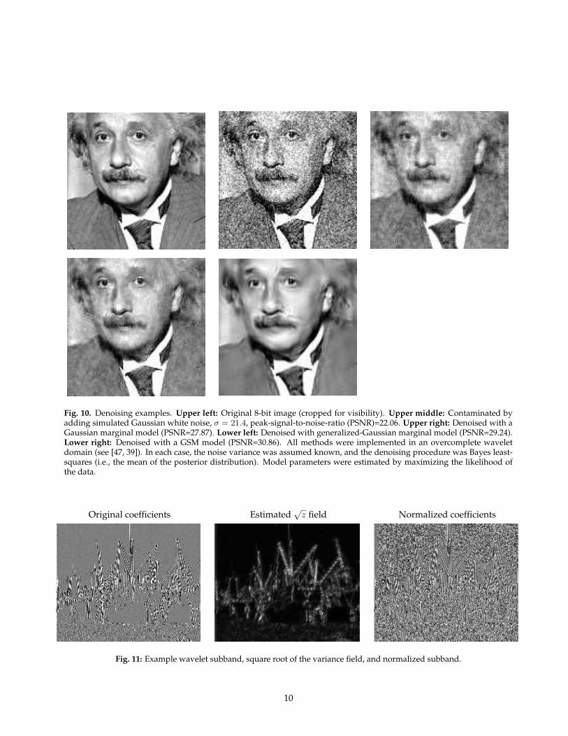
Fig. 10. Denoising examples. Upper left: Original 8-bit image (cropped for visibility). Upper middle: Contaminated byadding simulated Gaussian white noise, σ = 21.4, peak-signal-to-noise-ratio (PSNR)=22.06. Upper right: Denoised with aGaussian marginal model (PSNR=27.87). Lower left: Denoised with generalized-Gaussian marginal model (PSNR=29.24).Lower right: Denoised with a GSM model (PSNR=30.86). All methods were implemented in an overcomplete waveletdomain (see [47, 39]). In each case, the noise variance was assumed known, and the denoising procedure was Bayes least-squares (i.e., the mean of the posterior distribution). Model parameters were estimated by maximizing the likelihood ofthe data.

Original coefficients Estimated√

z field Normalized coefficients

Fig. 11: Example wavelet subband, square root of the variance field, and normalized subband.

10

−50 0 5010

0

105

−50 0 5010

0

105

(a) Observed (b) Simulated

(c) Observed (d) Simulated

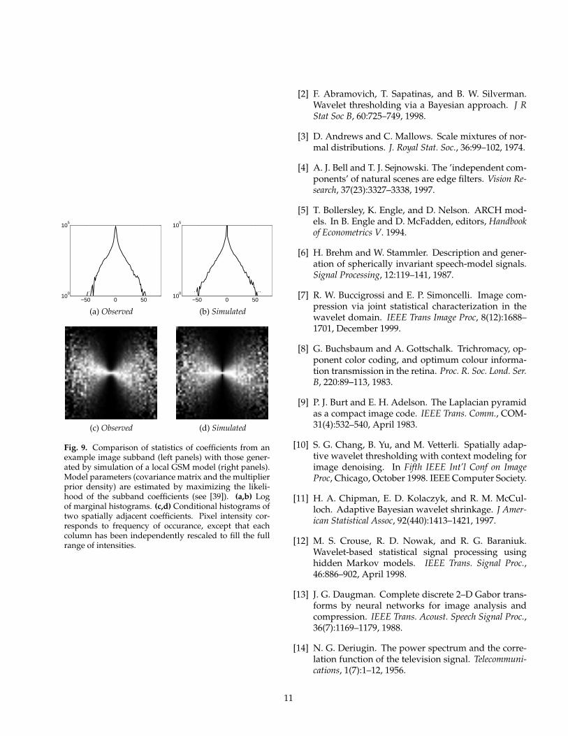
Fig. 9. Comparison of statistics of coefficients from anexample image subband (left panels) with those gener-ated by simulation of a local GSM model (right panels).Model parameters (covariance matrix and the multiplierprior density) are estimated by maximizing the likeli-hood of the subband coefficients (see [39]). (a,b) Logof marginal histograms. (c,d) Conditional histograms oftwo spatially adjacent coefficients. Pixel intensity cor-responds to frequency of occurance, except that eachcolumn has been independently rescaled to fill the fullrange of intensities.

[2] F. Abramovich, T. Sapatinas, and B. W. Silverman.Wavelet thresholding via a Bayesian approach. J RStat Soc B, 60:725–749, 1998.

[3] D. Andrews and C. Mallows. Scale mixtures of nor-mal distributions. J. Royal Stat. Soc., 36:99–102, 1974.

[4] A. J. Bell and T. J. Sejnowski. The ’independent com-ponents’ of natural scenes are edge filters. Vision Re-search, 37(23):3327–3338, 1997.

[5] T. Bollersley, K. Engle, and D. Nelson. ARCH mod-els. In B. Engle and D. McFadden, editors, Handbookof Econometrics V. 1994.

[6] H. Brehm and W. Stammler. Description and gener-ation of spherically invariant speech-model signals.Signal Processing, 12:119–141, 1987.

[7] R. W. Buccigrossi and E. P. Simoncelli. Image com-pression via joint statistical characterization in thewavelet domain. IEEE Trans Image Proc, 8(12):1688–1701, December 1999.

[8] G. Buchsbaum and A. Gottschalk. Trichromacy, op-ponent color coding, and optimum colour informa-tion transmission in the retina. Proc. R. Soc. Lond. Ser.B, 220:89–113, 1983.

[9] P. J. Burt and E. H. Adelson. The Laplacian pyramidas a compact image code. IEEE Trans. Comm., COM-31(4):532–540, April 1983.

[10] S. G. Chang, B. Yu, and M. Vetterli. Spatially adap-tive wavelet thresholding with context modeling forimage denoising. In Fifth IEEE Int’l Conf on ImageProc, Chicago, October 1998. IEEE Computer Society.

[11] H. A. Chipman, E. D. Kolaczyk, and R. M. McCul-loch. Adaptive Bayesian wavelet shrinkage. J Amer-ican Statistical Assoc, 92(440):1413–1421, 1997.

[12] M. S. Crouse, R. D. Nowak, and R. G. Baraniuk.Wavelet-based statistical signal processing usinghidden Markov models. IEEE Trans. Signal Proc.,46:886–902, April 1998.

[13] J. G. Daugman. Complete discrete 2–D Gabor trans-forms by neural networks for image analysis andcompression. IEEE Trans. Acoust. Speech Signal Proc.,36(7):1169–1179, 1988.

[14] N. G. Deriugin. The power spectrum and the corre-lation function of the television signal. Telecommuni-cations, 1(7):1–12, 1956.

11

[15] D. W. Dong and J. J. Atick. Statistics of natural time-varying images. Network: Computation in Neural Sys-tems, 6:345–358, 1995.

[16] J. H. Elder and R. M. Goldberg. Ecological statis-tics of gestalt laws for the perceptual organization ofcontours. Journal of Vision, 2(4):324–353, 2002. DOI10:1167/2.4.5.

[17] J. H. Elder and S. W. Zucker. Local scale control foredge detection and blur estimation. IEEE Pat. Anal.Mach. Intell., 20(7):699–716, 1998.

[18] D. J. Field. Relations between the statistics of naturalimages and the response properties of cortical cells.J. Opt. Soc. Am. A, 4(12):2379–2394, 1987.

[19] W. S. Geisler, J. S. Perry, B. J. Super, and D. P. Gal-logly. Edge co-occurance in natural images pre-dicts contour grouping performance. Vision Research,41(6):711–724, March 2001.

[20] D. Heeger and J. Bergen. Pyramid-based textureanalysis/synthesis. In Proc. ACM SIGGRAPH, pages229–238. Association for Computing Machinery, Au-gust 1995.

[21] P. Hoyer and A. Hyvarinen. A multi-layer sparsecoding network learns contour coding from naturalimages. Vision Research, 42(12):1593–1605, 2002.

[22] J. Huang and D. Mumford. Statistics of natural im-ages and models. In CVPR, page Paper 216, 1999.

[23] A. Hyvarinen and P. Hoyer. Emergence of topog-raphy and complex cell properties from natural im-ages using extensions of ICA. In S. A. Solla, T. K.Leen, and K.-R. Muller, editors, Adv. Neural Informa-tion Processing Systems, volume 12, pages 827–833,Cambridge, MA, May 2000. MIT Press.

[24] A. Hyvarinen, J. Hurri, and J. Vayrynen. Bubbles: Aunifying framework for low-level statistical proper-ties of natural image sequences. J. Opt. Soc. Am. A,20(7), July 2003.

[25] E. T. Jaynes. Where do we stand on maximum en-tropy? In R. D. Levine and M. Tribus, editors, TheMaximal Entropy Formalism. MIT Press, Cambridge,MA, 1978.

[26] Y. Karklin and M. S. Lewicki. Learning higher-orderstructures in natural images. Network, 14:483–499,2003.

[27] P. Kovesi. Image features from phase congruency.Videre: Journal of Computer Vision Research, 1(3), Sum-mer 1999.

[28] J. S. Lee. Digital image enhancement and noise fil-tering by use of local statistics. IEEE Pat. Anal. Mach.Intell., PAMI-2:165–168, March 1980.

[29] S. M. LoPresto, K. Ramchandran, and M. T. Orchard.Wavelet image coding based on a new generalizedGaussian mixture model. In Data Compression Conf,Snowbird, Utah, March 1997.

[30] M. Malfait and D. Roose. Wavelet-based image de-noising using a Markov random field a priori model.IEEE Trans. Image Proc., 6:549–565, April 1997.

[31] S. G. Mallat. A theory for multiresolution signal de-composition: The wavelet representation. IEEE Pat.Anal. Mach. Intell., 11:674–693, July 1989.

[32] S. G. Mallat. Zero-crossings of a wavelet transform.IEEE Trans. Info. Theory, 37(4):1019–1033, July 1991.

[33] M. K. Mihcak, I. Kozintsev, K. Ramchandran, andP. Moulin. Low-complexity image denoising basedon statistical modeling of wavelet coefficients. IEEETrans. Sig. Proc., 6(12):300–303, December 1999.

[34] P. Moulin and J. Liu. Analysis of multiresolutionimage denoising schemes using a generalized Gaus-sian and complexity priors. IEEE Trans. Info. Theory,45:909–919, 1999.

[35] B. A. Olshausen and D. J. Field. Emergence ofsimple-cell receptive field properties by learning asparse code for natural images. Nature, 381:607–609,1996.

[36] B. A. Olshausen and D. J. Field. Sparse coding withan overcomplete basis set: A strategy employed byV1? Vision Research, 37:3311–3325, 1997.

[37] A. V. Oppenheim and J. S. Lim. The importance ofphase in signals. Proc. of the IEEE, 69:529–541, 1981.

[38] J. Portilla and E. P. Simoncelli. A parametric texturemodel based on joint statistics of complex waveletcoefficients. Int’l Journal of Computer Vision, 40(1):49–71, December 2000.

[39] J. Portilla, V. Strela, M. Wainwright, and E. P. Simon-celli. Image denoising using a scale mixture of Gaus-sians in the wavelet domain. IEEE Trans Image Pro-cessing, 12(11):1338–1351, November 2003.

[40] J. Romberg, H. Choi, and R. Baraniuk. Bayesianwavelet domain image modeling using hiddenMarkov trees. In Proc. IEEE Int’l Conf on Image Proc,Kobe, Japan, October 1999.

12

[41] D. L. Ruderman. The statistics of natural images.Network: Computation in Neural Systems, 5:517–548,1996.

[42] D. L. Ruderman and W. Bialek. Statistics of natu-ral images: Scaling in the woods. Phys. Rev. Letters,73(6):814–817, 1994.

[43] D. L. Ruderman, T. W. Cronin, and C.-C. Chiao.Statistics of cone responses to natural images: Im-plications for visual coding. J. Opt. Soc. Am. A,15(8):2036–2045, 1998.

[44] J. Shapiro. Embedded image coding using ze-rotrees of wavelet coefficients. IEEE Trans Sig Proc,41(12):3445–3462, December 1993.

[45] M. Sigman, G. A. Cecchi, C. D. Gilbert, and M. O.Magnasco. On a common circle: Natural scenesand Gestalt rules. Proc. National Academy of Sciences,98(4):1935–1940, 2001.

[46] E. P. Simoncelli. Statistical models for images:Compression, restoration and synthesis. In Proc31st Asilomar Conf on Signals, Systems and Com-puters, pages 673–678, Pacific Grove, CA, Novem-ber 1997. IEEE Computer Society. Available fromhttp://www.cns.nyu.edu/∼eero/publications.html.

[47] E. P. Simoncelli. Bayesian denoising of visual im-ages in the wavelet domain. In P. Muller and B. Vi-dakovic, editors, Bayesian Inference in Wavelet BasedModels, chapter 18, pages 291–308. Springer-Verlag,New York, 1999. Lecture Notes in Statistics, vol. 141.

[48] E. P. Simoncelli and E. H. Adelson. Noise removalvia Bayesian wavelet coring. In Third Int’l Confon Image Proc, volume I, pages 379–382, Lausanne,September 1996. IEEE Sig Proc Society.

[49] A. Srivastava, X. Liu, and U. Grenander. Univer-sal analytical forms for modeling image probability.IEEE Pat. Anal. Mach. Intell., 28(9), 2002.

[50] D. J. Tolhurst, Y. Tadmor, and T. Chao. Amplitudespectra of natural images. Opth. and Physiol. Optics,12:229–232, 1992.

[51] A. Turiel, G. Mato, N. Parga, and J. P. Nadal. Theself-similarity properties of natural images resemblethose of turbulent flows. Phys. Rev. Lett., 80:1098–1101, 1998.

[52] A. Turiel and N. Parga. The multi-fractal structureof contrast changes in natural images: From sharpedges to textures. Neural Computation, 12:763–793,2000.

[53] A. van der Schaaf and J. H. van Hateren. Modellingthe power spectra of natural images: Statistics andinformation. Vision Research, 28(17):2759–2770, 1996.

[54] M. J. Wainwright and E. P. Simoncelli. Scale mixturesof Gaussians and the statistics of natural images. InS. A. Solla, T. K. Leen, and K.-R. Muller, editors, Adv.Neural Information Processing Systems (NIPS*99), vol-ume 12, pages 855–861, Cambridge, MA, May 2000.MIT Press.

[55] M. J. Wainwright, E. P. Simoncelli, and A. S. Will-sky. Random cascades on wavelet trees and theiruse in modeling and analyzing natural imagery. Ap-plied and Computational Harmonic Analysis, 11(1):89–123, July 2001.

[56] Z. Wang and E. P. Simoncelli. Local phase coherenceand the perception of blur. In S. Thrun, L. Saul, andB. Scholkopf, editors, Adv. Neural Information Process-ing Systems (NIPS*03), volume 16, Cambridge, MA,2004. MIT Press.

[57] A. P. Witkin. Scale-space filtering. In Proc. Intl. JointConf. Artificial Intelligence, pages 1019–1021, 1985.

[58] C. Zetzsche and E. Barth. Fundamental limitsof linear filters in the visual processing of two-dimensional signals. Vision Research, 30:1111–1117,1990.

[59] C. Zetzsche, B. Wegmann, and E. Barth. Nonlinearaspects of primary vision: Entropy reduction beyonddecorrelation. In Int’l Symposium, Society for Informa-tion Display, volume XXIV, pages 933–936, 1993.

[60] S.-C. Zhu. Statistical modeling and conceptualiza-tion of visual patterns. IEEE Trans PAMI, 25(6), June2003.

[61] S. C. Zhu, Y. N. Wu, and D. Mumford. Minimax en-tropy principle and its application to texture model-ing. In Neural Computation, volume 9, pages 1627–1660, 1997.

[62] S. C. Zhu, Y. N. Wu, and D. Mumford. FRAME: Fil-ters, random fields and maximum entropy – towardsa unified theory for texture modeling. Intl. J. Comp.Vis., 27(2):1–20, 1998.

13