Embed Size (px)
Citation preview

1
Paper 456-2013
Exploring Time Series Data Properties in SAS®
David Maradiaga, Louisiana State University
Aude Pujula, Louisiana State University
Hector Zapata, Louisiana State University
ABSTRACT
Box and Jenkins popularized graphical methods for studying time series properties of time series data. Dickey-and Fuller did the same for unit-root tests. Both methods seek to understand the non-stationary properties of data and SAS® is a popular software used by applied researchers. The purpose of this paper is to provide a series of steps using SAS MACRO Language, PROC SGPANEL, ARIMA, AUTOREG, and %DFTEST to diagnose non-stationary properties of data. A comparison among three competing SAS procedures is presented with SAS capabilities highlighted using simulated time series.
INTRODUCTION
Times series data such as asset prices, currency exchange rates, exports, gross domestic product, and consumer price index are commonly used by banks, financial, economic policy and marketing research institutions to forecast prices, predict supply and demand of products and services. Because several predictive models work under the stationary assumption, spurious results are possibly obtained when using non-stationary time series.
Time series data with changing means and variances are referred as non-stationary (Hamilton, 1994). One of the processes that is often associated with such data is a random walk, meaning that the series behaves in an unpredictable pattern similar to that of an winding road. In empirical modeling, such series tend to cause estimation, inference and forecasting problems. Granger and Newbold (1974), for example, showed than when running a regression with two variables that behave as random walks, spurious results are possible. In order to attain consistent and reliable results, the consensus in the literature has been to use filtering techniques to appropriately transform non-stationary data into stationary. Simply stated, the goal is to convert the unpredictable process to one that has a mean returning to a long term average and a variance that does not depend on time.
The literature recommends that one must be familiar with the type of non-stationary process before embarking in the use of filtering techniques. Non-stationary processes include deterministic trends ), and stochastic
trends ( ). Notice that a deterministic trend can be visualized for financial time series as an up-trending
process with fluctuations within a constant variance. Examples of stochastic trends are: pure random walk ( ), random walk with drift , and random walk with drift and trend ( ). At the expense of oversimplification, a random walk (also referred as a unit-root process) can be thought of as a process with trends whose slope and direction change in an unpredictable manner making modeling and forecasting unfeasible (figure 1).
The usual convention in the literature is to transform deterministic trends using detrending (demeaning) and stochastic trends with differences or ARIMA filters. Hamilton (1994) is an advocate of the necessity to correctly transform deterministic trends and unit-root processes in order to avoid misleading results. Enders (2004) also insists on this important fact by claiming that: “the form of the trend has important implications for the appropriate transformation to attain a stationary series.” Via Monte Carlo studies Zapata and Rambaldi (1989) found that arbitrary transformations to commodity prices and crop yields data in some instances generate series with different properties than those of the underlying stochastic process. According to Hamilton (1994) and Enders (2004) if time series has a unit-root, then applying first differences produces a stationary series. However, when a deterministic trend process ( ), is first-differenced a unit-root is introduced into the moving average component Conversely, if a random walk process with drift is detrended, then the time-dependence of the mean
is successfully remedied, but not for the variance, thus failing to transform into a stationary series. Thus, proper identification of the properties of a time series is essential in empirical work.
The purpose of this paper is to provide an easy way to recognize the different time series processes in order to apply the appropriate remedies to obtain reliable results in statistical models that depend on the stationary assumption. DATA steps are used to simulate times series data. PROC SGPLOT and PROC SGPANEL are used to create graphs from the Monte Carlo simulated data. PROC ARIMA, AUTOREG, and %DFTEST are used to unveil the type of processes of times series data. DATA steps and PROC REG are provided to transform non-stationary data into stationarity series. The proposed steps herein could be of help to a practitioner engaged in empirical model building with time series data. The contribution of this work should be of value to a broad audience (and fields) given that time series data are often used in economic and business forecasting, financial analysis, and public policy analyses.
Statistics and Data AnalysisSAS Global Forum 2013

2
EXAMPLE OF SPURIOUS REGRESSION RESULTS
Granger and Newbold (1974); Enders (2004); and Hill, Griffiths and Lim (2011) provide excellent illustrations of spurious regression results when working with non-stationary times series that are not related. To motivate the discussion of the present paper, a similar example is presented. Two non-stationary series were generated independently (random walks: RW1 and RW2). The generated series are plotted in figure1. They seem to be related as they fluctuate in a similar manner over time. Indeed, the results of a linear regression of RW1 on RW2 are: a slope coefficient with a significant t-statistic (p-value <0.0001) and a high goodness of fit (R
2 = 0.71). Nevertheless, by
fitting a regression using non-stationary data, the least squares assumptions that the errors have a zero mean and finite variance are violated. Therefore, the least squares are not consistent and test of statistical inference do not hold. Granger and Newbold (1974) coined the term “spurious regression” to a regression of non-stationary unrelated variables that yields a high R
2 and apparently significant t-statistics. In an attempt to demonstrate that there is no
relationship between these two variables, the data are transformed into stationary series so that the OLS estimator has its usual properties. The results clearly show that there no statistical meaningful relationship between the two variables (p-value 0.62 and R
2 = 0.005).
Figure 1. Seemingly Related Variables
METHODOLOGY
The objective of this paper is to provide a list of steps under different procedures in Base SAS® to diagnose the time series properties of data. The proposed approach consists of the following steps. Times series are generated via Monte Carlo simulation. DATA step was used to simulate different data generating processes (DGP hereafter) that are commonly found in economic and financial data. PROC SGPLOT and PROCSGPANEL are used to generate graphs of the simulated series for a visual inspection that gives a notion of the DGP of the series. A comparison of Dickey-Fuller unit-root tests (ADF hereafter) option in Base SAS® PROC ARIMA, PROC AUTOREG, and %DFTEST is provided. Some DATA Steps and PROC REG codes are used to transform non-stationary data into stationary series. At the end of the paper a summary, implications and conclusions section is provided.
DATA
The analysis uses time series Monte Carlo simulated data. DATA step was used to generate time series processes which mimic the behavior of economic and financial data such as gross domestic product, Inflation rates, and federal funds rates. Using DATA steps, seven different data processes were simulated: white noise (WN), trend stationary (TS), random walk (RW), random walk with drift (RWD) random walk with drift and trend (RWDT), ARMA, and
ARIMA. Each process was simulated for 100 observations and 1,000 replications as shown below. The simulated data are plotted in figure 2.
OLS with Non-Stationary Variables
OLS with Stationary Variables
Statistics and Data AnalysisSAS Global Forum 2013

3
White Noise (WN):
DATA wn;
Process='I White Noise';
DO nsam=1 to 1000;
SEED=1564646+nsam;
DO i=1 TO 200;
error=RANNOR(SEED);
y=2+error;
IF i>100 THEN OUTPUT;
END;
END;
RUN;
Trend Stationary (TS):
DATA ts;
Process='II Trend';
DO nsam=1 TO 1000;
SEED=1564646+nsam;
a0=2;
a2=0.8;
DO i=1 TO 200;
error=RANNOR(SEED);
y= a0 + i*a2 + error;
IF i>100 THEN OUTPUT;
END;
END;
RUN; Random Walk (RW):
DATA rw;
Process='III RW';
DO nsam=1 TO 1000;
SEED=1564646+nsam;
y=0;
DO i=1 TO 200;
error=RANNOR(SEED);
y= y+ error;
IF i>100 THEN OUTPUT;
END;
END;
RUN;
Random Walk with Drift (RWD):
DATA rwd;
DO nsam=1 TO 1000;
SEED=1564646+nsam;
a0=0.2;
y=0;
DO i=1 TO 200;
error=RANNOR(SEED);
y= a0 + y + error;
IF i>100 THEN OUTPUT;
END;
END;
RUN;
RWDT:
DATA rwdt;
Process='V RWDT';
DO nsam=1 TO 1000;
SEED=1564646+nsam;
a0=0.2;
a2=0.2;
y=0;
DO i=1 TO 200;
error=RANNOR(SEED);
y= a0 + y + a2*i - a2*(i-2) +error;
IF i>100 THEN OUTPUT;
END;
END;
RUN;
ARMA:
DATA arma;
Process='VI ARMA';
DO nsam=1 TO 1000;
SEED=1564646+nsam;
y1=0; e1=0; e=0; y=0;
*y1=yt-1 e=et e1=et-1;
DO i=1 TO 200;
y1=y;e1=e;
e=RANNOR(SEED);
y= 1+ 0.7*y1 + e + 0.5*e1;
IF i>100 THEN OUTPUT;
END;
END;
RUN;
ARIMA:
DATA arima;
Process='VII ARIMA';
DO nsam=1 TO 1000;
SEED=1564646+nsam;
y1=0; e1=0; e=0; y=0;
*y1=yt-1 e=et e1=et-1;
DO i=1 TO 200;
y1=y;e1=e;
e=RANNOR(SEED);
y= 1*y1 + e + 0.5*e1;
IF i>100 THEN OUTPUT;
END;
END;
RUN;
CONCATENATING DATASETS:
DATA All_Processes (WHERE =(nsam IN(1)));
SET wn ts rw rwd rwdt arma arima;
d=i+1810;
TY=y;
RUN;
PLOTTING THE SIMULATED SERIES:
ODS GRAPHICS /IMAGEFMT=JPEG HEIGHT=8.75in
WIDTH = 6.5in ANTIALIASMAX=1500;
PROC SGPANEL DATA= All_Processes;
PANELBY Process /ONEPANEL UNISCALE=COLUMN
LAYOUT=ROWLATTICE NOVARNAME;
REG x=d y=Ty/ CLM;
SERIES x=d y=TY;
RUN;
Statistics and Data AnalysisSAS Global Forum 2013

4
Figure 2. Simulated Time Series
Statistics and Data AnalysisSAS Global Forum 2013

5
VISUAL INSPECTION
Visual inspection is based on the classical method of Box-Jenkins (1970) for identifying properties of time series data. Also Hill, Griffiths and Lim (2011, p. 486) recommend to plot the series to have a first impression about the Data Generating Process. When having first glance to the graphs, plotted in figure 2, we are interested in finding data behaviors that could violate the stationary assumption. That is looking for series that always come back to the mean, have an equal variance and the covariance between any two values in the series depend solely in the interval of time that separates them. For example, when looking at the white noise process in figure 2, we can easily see that this process fulfills the requirements for the stationary assumption; it has fluctuations that always come back to a mean of 2 and a constant variance (between 0 and 4 in figure 2). Thus, no transformation of the data will be needed. In the second process, trend stationary, it is visible that the mean is changing over time while the series fluctuates within an equal variance. Hence, in order to have reliable results in some statistical estimators such as OLS that depend on the stationarity assumption, the series need to be transformed into stationary by “de-trending.” In the case of stochastic trend processes (e.g. random walk, random walk with drift, and random walk with drift and trend), it is hard to tell by a simple visual inspection. Let’s assume that you are provided with the same data, but only for the 1960 to 1980 period (figure 2). Then you will think of a RW and RWD as having a simple linear downward sloping trend, while RWDT seems to behave like a white noise process over the same period of time. In reality these three processes do not have a constant mean and variance and therefore violate the stationarity assumption. The most common remedy is a data transformation like differencing or ARIMA filters. Because visual inspection only offers an initial guess about the DGP, the next section of the paper is dedicated to a confirmatory analysis via statistical tests of stationarity, offering a more reliable technique to profile series.
SUMMARY OF AUGMENTED DICKEY-FULLER UNIT-ROOT TEST FOR STATIONARITY
The ADF test procedure is based in the estimation of three equations (steps) that are used to test the presence of: (1) a unit-root with a constant and a trend, (2) a unit-root with a constant and (3) a simple unit-root process. SAS PROC ARIMA, PROC AUTOREG, and %DFTEST can be implemented following that systematic set of steps.
ADF tests actually correspond to three regression equations that differ from the presence of deterministic terms. The choice often depends on the nature of the DGP. However, when the DGP is unknown, a common strategy is to start with the most general equation (1) and estimate it using ordinary least squares (OLS).
(1)
This is a regression of first-differenced series ( ) on a constant term ( ), a linear trend ( ), lagged levels ( )
and augmented with lagged differences ( ) to capture the whole dynamic nature of the process and fix
autocorrelation of the residuals. The optimal number of lags is chosen by ranking models based on the lowest estimate for the Akaike’s information criterion (Akaike, 1974).
The null hypothesis is that the time series is generated from a unit-root process (Ho: γ=0) which is tested using the ττ statistic. Alternatively, it is possible to carry out a joint test for the significance of the trend and the presence of a unit-root (Ho: a2=γ=0) using the φ3 statistic (the F-test in the SAS output for Type Trend). If the null is rejected, it is concluded that the series is generated from a trend stationary process.
If the restriction is not binding, we proceed to the second step which is a unit root test using a regression with a drift only (2).
(2)
A joint test for the significance of the constant term and a unit-root is carried out (Ho: a0=γ=0) using the φ1 statistic (the F-test in the SAS output for Type Single Mean). If we fail to reject the null then the third step is executed which corresponds to a unit root test estimating a regression without deterministic terms (3).
(3)
The null of a unit root (Ho: γ=0) is tested using the τ statistic (the Tau Statistic in SAS output for Type Zero Mean). If
the null is rejected it is concluded that the series is generated from a stationary or white noise process. Otherwise, we can conclude that the series comes from a non-stationary process (e.g., random walk).
RESULTS
ADF UNIT ROOT TESTS IN SAS
In SAS there are several ways to carry out unit-root tests. We compare three procedures: PROC ARIMA, PROC AUTOREG, and the Macro %DFTEST. The three procedures have different options and some of the features may be relevant depending upon the situation a practitioner is facing. Procedures were executed using simulated data and the outputs are provided for comparison and discussion.
Statistics and Data AnalysisSAS Global Forum 2013
6
The ARIMA Procedure
PROC ARIMA DATA=All_Processes;
IDENTIFY VAR=TY NLAG=24
STATIONARITY=(ADF=(3));
BY Process;
RUN;
Although the code above produces unit-root tests for the seven data sets (processes), results are shown only for the case of a random walk series (TY) using the three different procedures.
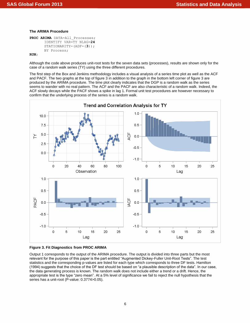
The first step of the Box and Jenkins methodology includes a visual analysis of a series time plot as well as the ACF and PACF. The two graphs at the top of figure 3 in addition to the graph in the bottom left corner of figure 3 are produced by the ARIMA procedure. The time plot clearly indicates that the DGP is a random walk as the series seems to wander with no real pattern. The ACF and the PACF are also characteristic of a random walk. Indeed, the ACF slowly decays while the PACF shows a spike in lag 1. Formal unit test procedures are however necessary to confirm that the underlying process of the series is a random walk.
Figure 3. Fit Diagnostics from PROC ARIMA
Output 1 corresponds to the output of the ARIMA procedure. The output is divided into three parts but the most relevant for the purpose of this paper is the part entitled “Augmented Dickey-Fuller Unit-Root Tests”. The test statistics and the corresponding p-values are listed for each type which corresponds to three DF tests. Hamilton (1994) suggests that the choice of the DF test should be based on “a plausible description of the data”. In our case, the data generating process is known. The random walk does not include either a trend or a drift. Hence, the appropriate test is the type “zero mean”. At a 5% level of significance we fail to reject the null hypothesis that the series has a unit-root (P-value: 0.3774>0.05).
Statistics and Data AnalysisSAS Global Forum 2013

7
Name of Variable = TY Mean of Working Series 4.323134 Standard Deviation 2.705826 Number of Observations 100
Autocorrelation Check for White Noise To
Lag Chi-Square DF Pr > ChiSq Autocorrelations
6 406.44 6 <.0001 0.918 0.866 0.821 0.779 0.728 0.673 12 526.06 12 <.0001 0.592 0.515 0.441 0.355 0.288 0.230 18 533.84 18 <.0001 0.142 0.100 0.037 -0.036 -0.103 -0.145 24 592.35 24 <.0001 -0.200 -0.232 -0.261 -0.296 -0.308 -0.320
Augmented Dickey-Fuller Unit Root Tests Type Lags Rho Pr < Rho Tau Pr < Tau F Pr > F Zero Mean 3 -1.2195 0.4349 -0.78 0.3774 Single Mean 3 -4.5611 0.4709 -1.44 0.5611 1.03 0.8085 Trend 3 -5.0778 0.8085 -1.57 0.7980 1.30 0.9158
Output 1. Output from PROC ARIMA
The AUTOREG Procedure
PROC AUTOREG DATA=All_Processes (WHERE=(process IN ('III RW')));
MODEL TY = / STATIONARITY=(ADF);
BY Process;
RUN;
Output 2 and figure 4 are produced by the above code. As in the ARIMA procedure the plots in figure 4 allows identifying characteristic behavior of a unit-root process. The second part of output 2 entitled “Augmented Dickey-Fuller Unit-Root tests” is identical to the test results in output 1.
Figure 4. Fit Diagnostics from PROC AUTOREG
Statistics and Data AnalysisSAS Global Forum 2013

8
Ordinary Least Squares Estimates SSE 732.149187 DFE 99 MSE 7.39545 Root MSE 2.71946 SBC 487.474288 AIC 484.869118 MAE 2.10615853 AICC 484.909934 MAPE 225.96573 HQC 485.923477 Durbin-Watson 0.1290 Regress R-Square 0.0000
Total R-Square 0.0000 Augmented Dickey-Fuller Unit Root Tests
Type Lags Rho Pr < Rho
Tau Pr < Tau F Pr > F
Zero Mean 3 -1.2195 0.4349 -0.7785 0.3774 Single Mean 3 -4.5611 0.4709 -1.4376 0.5611 1.0350 0.8085 Trend 3 -5.0778 0.8085 -1.5687 0.7980 1.2978 0.9158
Parameter Estimates Variable DF Estimate Standard
Error t Value Approx Pr
> |t|
Intercept 1 4.3231 0.2719 15.90 <.0001
Output 2. Output from PROC AUTOREG
%DFTEST
The last alternative is to use the %DFTEST macro. The code is given below and the output corresponds to output 3. The TREND=0 selects the DF test without trend and without drift. For a test with a drift only, we would have specified TREND=1 while TREND=2 is for a test with a drift and a deterministic trend.
%MACRO UR (DATANAME=, DATANAME2=, TREND=, OUTNAME=, TITLE=);
DATA &dataname2;
SET &dataname(WHERE=(nsam IN (1)));
TY=y;
RUN;
%DFTEST (&dataname2,TY,AR=3, TREND=&trend, OUTSTAT=&outname);
PROC PRINT DATA=&outname;
TITLE "&title";
RUN;
%MEND UR;
%UR(dataname=rw, dataname2=rw_lv, TREND=0, outname=dftest_rw, title=UR Test RW);
Obs TYPE STATUS DEPVAR NAME MSE Intercept AR_V DLAG_V
1 PARM 0 Conv AR_V 0.87 . -1 -0.014582
2 COV 0 Conv AR_V Intercept 0.87 . . 0.000351
3 COV 0 Conv AR_V DLAG_V 0.87 . . -0.000234
4 COV 0 Conv AR_V AR_V1 0.87 . . -0.000228
5 COV 0 Conv AR_V AR_V2 0.87 . . -0.000182
6 COV 0 Conv AR_V AR_V3 0.87 . . -0.014582
Output Continued
Obs AR_V1 AR_V2 AR_V3 NOBS TAU TREND DLAG PVALUE
1 -0.20707 -0.031567 0.090706 96 -0.77849 0 1 0.37739
2 -0.00023 -0.000228 -0.000182 96 -0.77849 0 1 0.37739
3 0.0101 0.002013 0.000143 96 -0.77849 0 1 0.37739
4 0.00201 0.010367 0.001644 96 -0.77849 0 1 0.37739
5 0.00014 0.001644 0.010033 96 -0.77849 0 1 0.37739
6 -0.20707 -0.031567 0.090706 96 -0.77849 0 1 0.37739
Output 3. Output from a %DFTEST
Statistics and Data AnalysisSAS Global Forum 2013
9
DATA TRANSFORMATIONS (FILTERS)
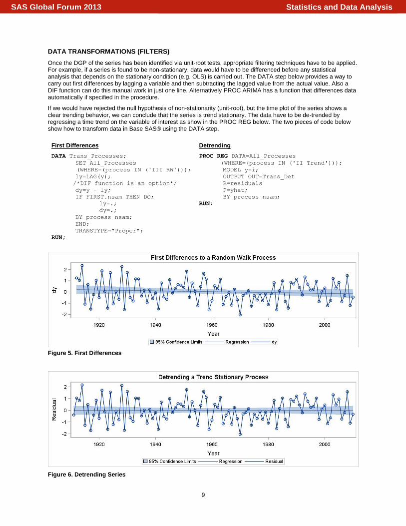
Once the DGP of the series has been identified via unit-root tests, appropriate filtering techniques have to be applied. For example, if a series is found to be non-stationary, data would have to be differenced before any statistical analysis that depends on the stationary condition (e.g. OLS) is carried out. The DATA step below provides a way to carry out first differences by lagging a variable and then subtracting the lagged value from the actual value. Also a DIF function can do this manual work in just one line. Alternatively PROC ARIMA has a function that differences data automatically if specified in the procedure.
If we would have rejected the null hypothesis of non-stationarity (unit-root), but the time plot of the series shows a clear trending behavior, we can conclude that the series is trend stationary. The data have to be de-trended by regressing a time trend on the variable of interest as show in the PROC REG below. The two pieces of code below show how to transform data in Base SAS® using the DATA step.
First Differences
DATA Trans_Processes;
SET All_Processes
(WHERE=(process IN ('III RW')));
ly=LAG(y);
/*DIF function is an option*/
dy=y - ly;
IF FIRST.nsam THEN DO;
ly=.;
dy=.;
BY process nsam;
END;
TRANSTYPE="Proper";
RUN;
Detrending
PROC REG DATA=All_Processes
(WHERE=(process IN ('II Trend')));
MODEL y=i;
OUTPUT OUT=Trans_Det
R=residuals
P=yhat;
BY process nsam;
RUN;
Figure 5. First Differences
Figure 6. Detrending Series
Statistics and Data AnalysisSAS Global Forum 2013

10
COMPARISON SUMMARY
Options PROC ARIMA PROC AUTOREG %DFTEST
Unit-Roots STATIONARITY=(ADF= AR
orders DLAG= s )
STATIONARITY=(ADF<=(...)>, PHILLIPS<=(...)> )
NEW UNIT-ROOT TESTS
N/A ERS<=(...)>, KPSS<=(...)>, NP
<=(...)> N/A
Automatic Lag Selection
This is a downside of PROC ARIMA. Lag selection is not automatically chosen. However, you can request by trial and error or by specifying a subsequent number of lag lengths followed by comas. For example the following code is going to estimate seven different models and compute their unit-root tests STATIONARITY=(ADF=(1,2,3,4,5,6,7));.
This is a nice feature in PROC AUTOREG. The number of lags to be selected in the final model are automatically chosen based on statistical criteria (e.g., AIC, BIC, etc). Automatic lag selection is the default. Setting model TY = /STATIONARITY=(ADF=5) allows the user to request a specific number of lags.
This is a downside of %dftest. Trial and error is more difficult than in the case of PROC ARIMA because partial autocorrelation graphs are not outputted.
Differencing data
A nice feature in PROC ARIMA is that it does not only allow the user to transform data (differencing), but also to carry out the tests with transformed data. The option for first differences is IDENTIFY VAR=TY(1).
Transformations need to be in the dataset beforehand.
Transformations need to be in the dataset beforehand.
Detrending data
The feature is not available. A data step will be required to carry out this task as shown in "Detrend all Processes."
Same as above. Same as above.
Forecasts It is very robust to forecast various types of models, ARIMA, ARMA etc.
Autoregressive models. The drawback is that the user has to modify the data by using data steps prior forecasting with AUTOREG
No forecasting option.
Output
Unit-Root + trend test
Yes Augmented Dickey-Fuller three equation models are used for testing.
Yes Yes
Unit-Root + constant test
Yes Yes Yes
Unit-Root test Yes Yes Yes
Histogram distribution of the residuals
The output does not provide a distribution plot of residuals.
It presents a distribution of the residuals.
No graphs are displayed.
Studendized residuals plot
No Yes No
Scatter Plot Yes Yes No
Cooks D Plot No Yes No
ACF Autocorrelation Functions are presented automatically by PROC ARIMA.
Yes No
PACF Partial Autocorrelation Functions are displayed.
Yes No
IACF Integrated ACF are shown. No No
Table 1. PROC ARIMA, PROC AUTOREG, and %DFTEST Comparison
Statistics and Data AnalysisSAS Global Forum 2013

11
CONCLUSION
The aim of this paper was to present a series of steps that can serve as guidance for Base SAS ® users dealing with time series data. Monte Carlo simulated data are used to show how to identify stationary and non-stationary series. A series of graphs are generated with PROC SGPLOT and PROC SGPANEL for visual inspection of the data. Then demonstrations on how to carry out test for unit roots using PROC ARIMA, AUTOREG, and %DFTEST are provided. After a comparison of these three SAS Base 9.3 procedures, PROC ARIMA emerges as the most complete procedure with options that allow easier identification of properties of non-stationary time series.
REFERENCES
1. Akaike, Hirotugu. “A new look at the statistical model identification.” IEEE Transactions on Automatic Control, 19(June, 1974):716–723.
2. Box, G. and G. Jenkins (1907). Time Series Analysis: Forecasting and Control, San Francisco: Holden-Day. 3. Dickey, D.A. and W.A. Fuller. “Distribution of the Estimators for Autoregressive Time Series with a Unit
Root.” Journal of the American Statistical Association, (1979):427–431. 4. Enders, W. Applied Econometric Time Series. Wiley Series in Probability and Mathematical Statistics. New York:
John Wiley & Sons, 2004. 5. Granger, C.W.J. and P. Newbod. “Spurious Regressions in Econometrics.” Journal of Econometrics 2 (1974)
111-120. 6. Hamilton, J.D. Models of Non-stationary Time Series. Time Series Analysis. Princeton, NJ: Princeton University
Press, 1994. 7. Hill, R.C., W.E. Griffiths and G.C. Lim. Principles of Econometrics Fourth Edition. Hoboken, NJ:
John Wiley & Sons, Inc, p758, 2011. 8. Zapata, H.O., and A.N. Rambaldi. “Effects of Data Transformation on Stochastic Properties of Economic Data,”
Paper presented at the annual meetings of the American Agricultural Economics Association, Baton Rouge, Louisiana, 1989.
ACKNOWLEDGEMENTS
As SAS® Student Ambassadors-2013 Award recipients, we express our gratitude to Dr. Julie Petlick for her support as SAS® Student Programs Manager. As SCSUG 2012 Scholarship recipients, we would like to thank Dr. Lisa Mendez for her immensurable support as Student Scholarship Coordinator. We would like to express our deepest appreciation to Mr. Kirk Paul Lafler who has been very inspiring, motivating, and an exceptional SAS® mentor. We would like to thank the ISDS and AgEcon departments at LSU, and especially to Dr. Joni Shreve for her valuable instruction, encouragement and support with statistics and SAS® Technologies. And last but not the least; we also thank Dr. P. Lynn Kennedy for his mentorship through the PhD Program.
CONTACT INFORMATION
Comments, questions, and additions are welcomed. Contact the authors at:
David I. Maradiaga PhD Student in Agricultural Economics and MS in Analytics Candidate
Louisiana State University 101 Martin D. Woodin Hall Baton Rouge, LA 70803 Email:[email protected]
Aude L.J. Pujula PhD Candidate in Agricultural Economics
Louisiana State University 101 Martin D. Woodin Hall Baton Rouge, LA 70803 Email:[email protected]
Hector O. Zapata Executive Director of International Programs
Louisiana State University 108 Hatcher Hall Baton Rouge, LA 70803 Email:[email protected]
Statistics and Data AnalysisSAS Global Forum 2013

12
TRADEMARKS
SAS® and all other SAS Institute Inc. product or service names are registered trademarks or trademarks of SAS Institute Inc. in the USA and other countries. ® Indicates USA registration. MS Office® is a registered trademark of the Microsoft Corporation.
Other brand and product names are registered trademarks or trademarks of their respective companies.
Statistics and Data AnalysisSAS Global Forum 2013

![Welcome to DrRacket, version 6.1 [3m]. Language: slideshow ...richter/11-7-2014.pdfNov 07, 2014 · 123 456 789 4 2 123 456 789 5 123 456 789 9 123 456 789 7 7 123 456 789 1 456 789](https://img.pdfslide.us/doc/110x75/5fd9df3a07c10b0ee2107e89/welcome-to-drracket-version-61-3m-language-slideshow-richter11-7-2014pdf.jpg)
![Untitled 2 [] · /01-!." *23-!." 456-!." *+,-!7" /01-!7" *23-!7" 456-!7" *+,-#!" /01-#!" *23-#!" 456-#!" *+,-##" /01-##" *23-##" 456-##" *+,-#$" /01-#$" *23-#$" 456-#$" *+,-#%" /01](https://img.pdfslide.us/doc/110x75/5f2f2b6ad0823628e27434f2/untitled-2-01-23-456-7-01-7.jpg)


![[Shinobi] Bleach 456](https://img.pdfslide.us/doc/110x75/568c521f1a28ab4916b56b3d/shinobi-bleach-456-56fbbc5543513.jpg)


