4.5 Planar Hamiltonian and related systemskouzn101/INLDS/Hamiltonian.pdf4.5 Planar Hamiltonian and related systems There is a special class of planar systems, for which a complete

146 CHAPTER 4. PLANAR ODE

4.5 Planar Hamiltonian and related systems

There is a special class of planar systems, for which a complete characterizationof phase portraits is possible and which appear in Classical Mechanics. Moreover,it is possible to draw some conclusions about generic small perturbations of suchsystems.

4.5.1 Hamiltonian systems with one degree of freedom

Let H = H(q, p) be a smooth (at least C2) function H : R⇥ R ! R. Define

Hq(q, p) =@H(q, p)

@q, Hp(q, p) =

@H(q, p)

@p.

Definition 4.21 A planar system

⇢q = Hp(q, p),p = �Hq(q, p),

(4.29)

is called a Hamiltonian system with one degree of freedom and Hamiltonian(or energy function) H.

Example 4.22 (Lotka-Volterra system revisited)

Consider once again the Lotka-Volterra system from Section 4.4.1:

⇢x = ax� bxy,y = �cy + dxy.

(4.30)

The linear scalingx = ⇠

0

⇠, y = ⌘0

⌘, t = ⌧0

⌧

with

⇠0

=a

d, ⌘

0

=a

b, ⌧

0

=1

a

reduces (4.30) to ⇢⇠ = ⇠ � ⇠⌘,⌘ = ��⌘ + ⇠⌘,

(4.31)

where ⇠ and ⌘ are the derivatives of ⇠ and ⌘ with respect to the new time ⌧ , and

� =c

a

is a new parameter. Introduce new coordinates in the positive quadrant R2

+

by theformulas: ⇢

q = ln ⇠,p = ln ⌘.

4.5. PLANAR HAMILTONIAN AND RELATED SYSTEMS 147

0 1 2 3 4 5 60

1

2

3

4

5

−1 0 1 2−3

−2

−1

0

1

2

p⌘

q⇠

Figure 4.18: Phase portraits of the Lotka-Volterra system in the (⇠, ⌘)- and (q, p)-coordinates.

One has

q =⇠

⇠= 1� ⌘ = 1� ep,

p =⌘

⌘= �� + ⇠ = �� + eq.

Thus, (4.31) is smoothly equivalent in R2

+

to the Hamiltonian system (4.29) with

H(q, p) = �q � eq + p� ep.

The transformation (⇠, ⌘) 7! (q, p) maps closed orbits of (4.31) in R2

+

onto closedorbits of (4.29) in R2, preserving their time parameterization (see Figure 4.18). 3

The following result explains why (4.29) is also called a conservative system (seealso Exercise 4.7.12).

Theorem 4.23 (Conservation of energy) The Hamiltonian H(q, p) is a constantof motion for the Hamiltonian system, i.e. H(q(t), p(t)) = const along solutions.

Proof: H = Hq q +Hpp = HqHp �HpHq = 0. 2

This theorem has as an immediate implication that any orbit of (4.29) belongsto a level set {(q, p) 2 R2 : H(q, p) = h} of the Hamiltonian function H. Next wecan deduce further implications from the geometry of such level sets. As illustratedin the lower half of Figure 4.19, a connected component of a level set is typicallyeither

- a single point (corresponding to a maximum or a minimum of H);

- a closed curve (these occur in families parametrized by the value of H; a strictmaximum or minimum is always surrounded by such a family);


- a number of points connected by curves (more on this case below).

Another direct consequence of (4.29) is that equilibria of a Hamiltonian systemcorrespond exactly to critical points of H. So on the one hand we can use theclassification of nondegenerate critical points into extrema (maxima and minima)and saddle points, and on the other hand we can use the classification of equilibriaaccording to their stability properties. How do these two ways of classificationcorrespond to each other ?

A first observation is that (4.29) cannot have asymptotically stable equilibria(nor asymptotically stable cycles). Indeed, if all orbits starting in a neighbourhoodof an equilibrium converge towards this equilibrium, then H must be constant onthis neighbourhood (since H is continuous and constant along orbits). So the entireneighbourhood must consist of equilibria, a contradiction.

As H is assumed to be C2, the Jacobian matrix at some equilibrium exists andis given by

A =

✓H0

qp H0

pp

�H0

qq �H0

qp

◆,

where the superscript indicates the evauation of all quantities at the equilibrium.Thus Tr A = H0

qp�H0

qp = 0 and the eigenvalues of A are either real and of oppositesign or purely imaginary, depending on the sign of

detA = H0

qqH0

pp � (H0

qp)2 6= 0.

If we consider the equilibrium as a critical point of H, we are led to consider theHessian matrix

B =

✓H0

qq H0

qp

H0

qp H0

pp

◆,

which has exactly the same determinant as A. When the determinant is positive, Hhas an extremum (a maximum if H0

pp < 0 and a minimum if H0

pp > 0). Thus, whenA has purely imaginary eigenvalues, the corresponding equilibrium is a (nonlinear)center surrounded by a family of periodic orbits. When the determinant is negative,H has a saddle point and A has one positive and one negative real eigenvalue. Thus,the equilibrium is also a saddle point in the sense of planar dynamical systems (sowhen locally a level set consists of two intersecting curves, these are exactly thelocal stable and the local unstable manifolds of the point of intersection, which is asaddle equilibrium point).

In order to formulate our conclusions as a lemma, it is useful to introduce a newterm.

Definition 4.24 An equilibrium is called simple, if it has no zero eigenvalue.

Lemma 4.25 A simple equilibrium of a Hamiltonian system (4.29) with one degreeof freedom is either a saddle or a center. The first case applies when

H0

qqH0

pp � (H0

qp)2 < 0

and the second when the opposite inequality holds. 2


Remarks:(1) With any smooth function H : R⇥R ! R one can also associate the gradient

flow generated by the system

⇢q = �Hq(q, p),p = �Hp(q, p).

(4.32)

For this flow H = �[(Hq)2 + (Hp)2] 0, so orbits converge towards minima of Hfollowing steepest descent and crossing level curves of H orthogonally.

(2) Returning to (4.29), we observe that one might wonder how the period variesas a function of the value of H when there is a family of closed orbits ? Is the perioda monotone function ? This is a notoriously di�cult problem. With considerablee↵ort one can prove monotonicity for some specific systems. But as far as we know,there is no general result and, in fact, the period may not be monotone for otherspecific systems.

(3) Finally note that the divergence of the vector field (Hp,�Hq)T is zero. Asa consequence, planar Hamiltonian flows preserve area (see Theorem 4.38 in theAppendix to this chapter for a general result). }

4.5.2 Potential systems with one degree of freedom

Definition 4.26 A planar system (4.29) with

H(q, p) =1

2p2 + U(q),

where U is a smooth scalar function, is called a potential system.

Here the term 1

2

p2 is called the kinetic energy, while U(q) is called the potentialenergy.

The corresponding Hamiltonian system (4.29) has the form:

⇢q = p,p = �U 0(q).

(4.33)

Eliminating p we get Newton’s 2nd Law:

q = F (q),

with the potential force F (q) = �U 0(q). (Side remark for physicists: Notice that the“mass” is put equal to one, which can always be achieved by scaling.)

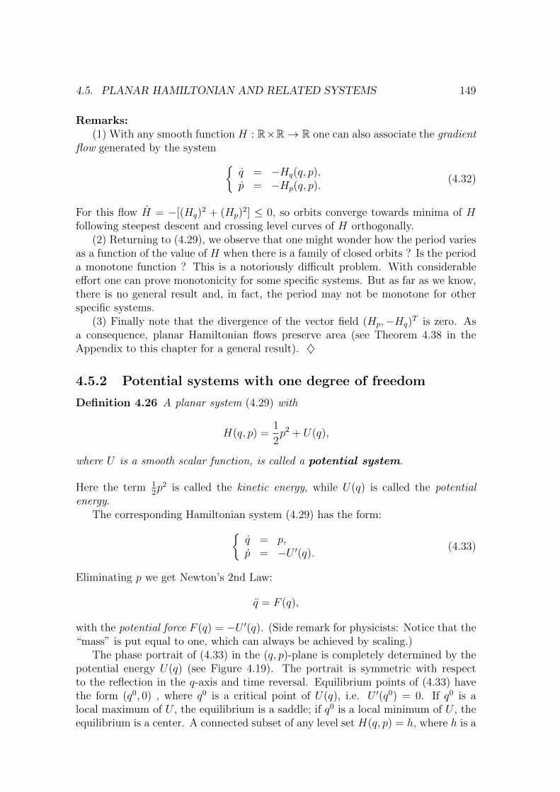
The phase portrait of (4.33) in the (q, p)-plane is completely determined by thepotential energy U(q) (see Figure 4.19). The portrait is symmetric with respectto the reflection in the q-axis and time reversal. Equilibrium points of (4.33) havethe form (q0, 0) , where q0 is a critical point of U(q), i.e. U 0(q0) = 0. If q0 is alocal maximum of U , the equilibrium is a saddle; if q0 is a local minimum of U , theequilibrium is a center. A connected subset of any level set H(q, p) = h, where h is a


U(q)

q

p

(1)

(2)

(3)

(1)(2)

(3) (3)

q1

q2

h

Figure 4.19: Newton dynamics with one degree of freedom.

regular value, is di↵eomorphic to either a circle (closed curve) or a line. The readeris invited to prove that any closed orbit defines a periodic solution with period

T =

Z q2

q1

s2

h� U(q)dq, (4.34)

where q1

< q2

are the coordinates of the intersections of the orbit with the q-axisand, therefore, U(q

1

) = U(q2

) = h (see also Exercise 4.7.11). Critical level setscontain equilibria and homo- or heteroclinic orbits, which are asymptotic to them.

Example 4.27 (Famous potential systems with m = 1)

(1) Harmonic oscillator:

H =1

2(p2 + q2).

(2) Ideal pendulum:

H =1

2p2 � cos q.

(3) Du�ng oscillator:

H =1

2(p2 � q2) +

q4

4.

You are invited to draw their phase portraits yourself. 3


4.5.3 Small perturbations of planar Hamiltonian systems

As we have seen in the previous sections, planar Hamiltonian systems have veryspecial phase portraits, which allow for rather detailed characterization. Can we usethis information to analyse planar systems which are not Hamiltonian but close tothem? One can think of a potential system subject to a small friction, or about ageneralized Lotka-Volterra model that takes into account weak competition amongprey or predators. As we shall see, the topology of the phase portrait of a Hamilto-nian system changes qualitatively under generic (non-Hamiltonian) perturbations:Centers become (stable or unstable) foci, while families of periodic orbits disappear,possible giving rise to (stable or unstable) limit cycles. Homoclinic orbits also disap-pear. These qualitative changes are examples of bifurcations of dynamical systems,which we will study systematically in Chapters 5,6, and 7.

First consider the following one-parameter perturbation of (4.29):

x =

✓Hx2(x)

�Hx1(x)

◆+ "f(x), x = (x

1

, x2

)T 2 R2, (4.35)

where " 2 R is a small parameter, and H : R2 ! R and f : R2 ! R2 are smoothfunctions. Since we are interested in non-Hamiltonian perturbations, divf does notvanish.

We begin with a simple result concerning equilibria.

Theorem 4.28 Consider the system (4.35) and assume that f(0) = 0.(i) If x = 0 is a simple saddle at " = 0, then x = 0 is a saddle of (4.35) for all "

with su�ciently small |"|.(ii) If x = 0 is a simple center at " = 0, then x = 0 is a focus of (4.35) for all "

with su�ciently small |"| > 0. Moreover, this focus is stable for " divf(0) < 0 andunstable for " divf(0) > 0.

Proof: Write the Jacobian matrix of (4.35) at the equilibrium x = 0 as

A(") =

✓H0

x1x2H0

x2x2

�H0

x1x1�H0

x2x1

◆+ "f 0

x .

Its eigenvalues �1,2(") depend smoothly on ".

Part (i) is then obvious, since if �1

(") and �2

(") have opposite sign at " = 0, thenthis property will hold for all su�ciently small ". Thus, by the Grobman-HartmanTheorem, x = 0 is a saddle for such parameter values.

When x = 0 is a center at " = 0, the matrix A(") has a pair of nonreal eigenvalues�1

= �2

(") for all su�ciently small " and

2Re �1,2(") = Tr A(") = "Tr f 0

x = " divf(0).

Applying the Grobman-Hartman Theorem for " 6= 0, we obtain Part (ii) of thetheorem. 2


Example 4.29 (Perturbed Lotka-Volterra system)

Consider the following small perturbation of the (scaled) Lotka-Volterra system(4.31): ⇢

⇠ = ⇠ � ⇠⌘ � "⇠2,⌘ = ��⌘ + ⇠⌘,

(4.36)

where 0 < " ⌧ 1, � > 0 and the "⇠2-term describes weak competition among prey.Introducing the same variables as in Example 4.22,

⇢q = ln ⇠,p = ln ⌘,

we obtain ⇢q = 1� ep � "eq,p = �� + eq.

This system has for (1� �") > 0 an equilibrium

(q0("), p0(")) = (ln �, ln(1� �")),

which is a center if " = 0. Translating the origin of the coordinate system to thisequilibrium by the transformation

⇢x1

= q � ln �,x2

= p� ln(1� "�),

we obtain the system⇢

x1

= 1� ex2 + "�(ex2 � ex1),x2

= ��(1� ex1),(4.37)

which has the form (4.35) with H(x) = x2

� ex2 + �(x1

� ex1) and

f(x) =

✓�(ex2 � ex1)

0

◆, f(0) = 0.

The system (4.37) satisfies the conditions of Theorem 4.28. Since

" divf(0) = �"� < 0,

the equilibrium (q0("), p0(")) is a stable focus for su�ciently small " > 0.Note that this result perfectly agrees with our analysis in Section 4.4.3, where it

was shown that system (4.13) has a unique positive globally asymptotically stableequilibrium when ad � ce > 0. Indeed, system (4.13) coincides with system (4.36)if we set a = b = d = 1, c = �, and e = ", so that the above condition turns into(1� "�) > 0, which is obviously true for small ". 3

Remark: Consider a slightly more general system

x =

✓Hx2(x)

�Hx1(x)

◆+ "f(x, "), x = (x

1

, x2

)T 2 R2, " 2 R, (4.38)


where H is smooth and has a nondegenerate critical point x = 0, while f is a smoothfunction of (x, "). The Implicit Function Theorem assures that (4.38) has a smoothfamily x0(") of equilibria for small " 6= 0, such that x0(0) = 0. Translating the originto x0("), we can assume without loss of generality that f(0, ") = 0 for all " withsmall |"|. Then, the equilibrium x = 0 is either a saddle or, when divf(0, 0) 6= 0, afocus. The stability of the focus is determined by the sign of divf(0, 0). }

Now we want to study limit cycles of the perturbed planar Hamiltonian system(4.35).

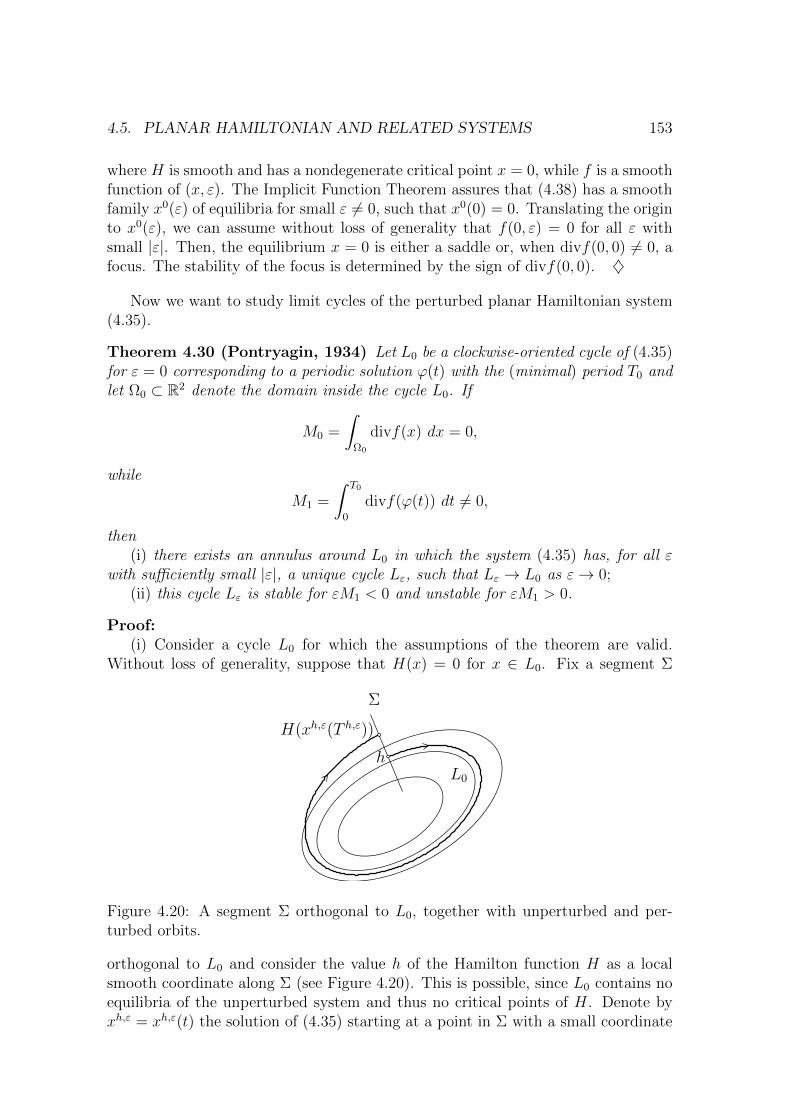
Theorem 4.30 (Pontryagin, 1934) Let L0

be a clockwise-oriented cycle of (4.35)for " = 0 corresponding to a periodic solution '(t) with the (minimal) period T

0

andlet ⌦

0

⇢ R2 denote the domain inside the cycle L0

. If

M0

=

Z

⌦0

divf(x) dx = 0,

while

M1

=

Z T0

0

divf('(t)) dt 6= 0,

then(i) there exists an annulus around L

0

in which the system (4.35) has, for all "with su�ciently small |"|, a unique cycle L", such that L" ! L

0

as " ! 0;(ii) this cycle L" is stable for "M

1

< 0 and unstable for "M1

> 0.

Proof:(i) Consider a cycle L

0

for which the assumptions of the theorem are valid.Without loss of generality, suppose that H(x) = 0 for x 2 L

0

. Fix a segment ⌃

L0

h

⌃

H(xh,"(T h,"))

Figure 4.20: A segment ⌃ orthogonal to L0

, together with unperturbed and per-turbed orbits.

orthogonal to L0

and consider the value h of the Hamilton function H as a localsmooth coordinate along ⌃ (see Figure 4.20). This is possible, since L

0

contains noequilibria of the unperturbed system and thus no critical points of H. Denote byxh," = xh,"(t) the solution of (4.35) starting at a point in ⌃ with a small coordinate


h, and let T h," be the minimal time needed by the solution to return back to ⌃.Due to the smooth dependence of solutions on the initial point and the parameter,T h," is a smooth function of (h, ") in a neighbourhood of (0, 0) with T 0,0 = T

0

, sincex0,0 = '.

Introduce another smooth function

�(h, ") = H(xh,"(T h,"))�H(xh,"(0)) = H(xh,"(T h,"))� h,

which one calls for obvious reasons the displacement function. In general, �(h, ") 6=0. However, �(h, 0) = 0, since H is constant along orbits of the unperturbedsystem. Moreover, if �(h, ") = 0, the perturbed system (4.35) has a closed orbitfor the corresponding value of " passing through the point in ⌃ with the coordinateh. We will analyse the equation �(h, ") = 0 with the help of the Implicit FunctionTheorem.

Along the solutions of (4.35), one has

�(h, ") =

Z Th,"

0

dH(xh,"(t)) =

Z Th,"

0

[Hx1(xh,"(t))xh,"

1

(t) +Hx2(xh,"(t))xh,"

2

(t)]dt

= "

Z Th,"

0

[Hx1(xh,"(t))f

1

(xh,"(t)) +Hx2(xh,"(t))f

2

(xh,"(t))] dt

= "

Z Th,0

0

[�xh,02

(t)f1

(xh,0(t)) + xh,01

(t)f2

(xh,0(t))] dt+O("2),

where the last integral is computed along solutions of (4.35) with " = 0. Since thesesolutions have clockwise orientation, we can write

�(h, ") = "M(h) +O("2), (4.39)

where

M(h) = �I

Lh

f1

dx2

� f2

dx1

=

Z

⌦h

divf(x) dx.

(The last equality, in which ⌦h is the domain inside the periodic orbit Lh belongingto the level curve H(x) = h, is Green’s formula (4.9); note the change of sign toincorporate the clockwise orientation of Lh.)

By assumption,

M(0) =

I

H(x)=0

f1

dx2

� f2

dx1

=

Z

⌦0

divf(x) dx = M0

= 0.

Thus we have

M(h) =

Z h

0

Z T s,0

0

divf(x(⌧, s))| det(J1

(⌧, s))| d⌧!ds,

where J1

is the Jacobian matrix of the map (⌧, h) 7! x(⌧, h) = xh,0(⌧). Hence

M 0(0) =

Z T 0,0

0

divf('(⌧)) |det(J1

(⌧, 0))| d⌧.


Di↵erentiating the identityH(xh,0(⌧)) = h

with respect to h, we obtain

Hx1(xh,0(⌧))

@xh,01

(⌧)

@h+Hx2(x

h,0(⌧))@xh,0

2

(⌧)

@h= 1.

Therefore,

det(J1

(⌧, h)) = det

0

BB@

@xh,01

(⌧)

@⌧

@xh,01

(⌧)

@h

@xh,02

(⌧)

@⌧

@xh,02

(⌧)

@h

1

CCA

= det

0

BB@Hx2(x

h,0(⌧))@xh,0

1

(⌧)

@h

�Hx2(xh,0(⌧))

@xh,02

(⌧)

@h

1

CCA = 1 .

Hence |det(J1

(⌧, 0))| = 1 and

M 0(0) =

Z T0

0

div f('(t)) dt = M1

6= 0

by the second assumption.Thus, we have

�(h, ") = "(M0

+ hM1

+O(h2)) +O("2) = "F (h, ")

for some smooth function F . If " = 0, � = 0 for all small |h| and all orbits areclosed (Hamiltonian case). If " 6= 0, the equation

F (h, ") = 0

is such that we can apply the Implicit Function Theorem. Indeed,

F (0, 0) = M0

= 0, Fh(0, 0) = M1

6= 0,

by the assumptions we made. Thus, there is a unique smooth function h = h("), h(0) =0, such that

F (h("), ") = 0

for all small |"|. This implies that �(h("), ") = 0 for all " with su�ciently small|"| 6= 0. Therefore, there exists a unique cycle L" through h(").

(ii) Since the map h 7! h+�(h, ") has derivative

1 +@�(h("), ")

@h


in the fixed point h(") and the sign of

@�(h("), ")

@h

coincides with the sign of "M1

, the stability assertions follow at once. 2

Remarks:(1) If L

0

has counter-clockwise orientation, the expression (4.39) will take theform

�(h, ") = �"M(h) +O("2).

The subsequent analysis can then be carried out with obvious modifications. Itshows that statement (i) is still valid, but the cycle L" is stable when "M

1

> 0 andunstable when "M

1

< 0.(2) When L

0

is oriented counter-clockwise,

I

L0

f1

(x)dx2

� f2

(x)dx1

=

Z T0

0

f('(t)) ^ '(t) dt,

where the wedge product of two vectors u, v 2 R2 is defined by u ^ v = u1

v2

� u2

v1

.3

Example 4.31 (Van der Pol equation)

The second-order equation,

x+ x = "x(1� x2), (4.40)

is called the van der Pol equation3. It can be rewritten as the equivalent planarsystem ⇢

x1

= x2

,x2

= �x1

+ "x2

(1� x2

1

).(4.41)

The system with " = 0 is Hamiltonian (harmonic oscillator) with H(x1

, x2

) =1

2

(x2

1

+ x2

2

), which has a family of 2⇡-periodic solutions

'(t) =

✓r sin tr cos t

◆, r > 0.

Since f1

= 0, f2

= x2

(1�x2

1

), and the periodic orbits are oriented clockwise, we get

M(r) = �I

x21+x2

2=r2f1

(x)dx2

�f2

(x)dx1

=

Z2⇡

0

r2 cos2 t(1�r2 sin2 t) dt =⇡

4r2(4�r2).

Therefore, M(r) = 0 for r = 2. Along this solution,

M1

=

Z2⇡

0

div f('(t)) dt =

Z2⇡

0

(1� 4 sin2 t)dt = �2⇡ < 0.

3van der Pol, B. ‘Forced oscillations in a circuit with nonlinear resistance (receptance withreactive triode)’, London, Edinburgh and Dublin Phil. Mag. 3 (1927), 65-80


x ’ = y

y ’ = − x + epsilon y (1 − x2)epsilon = 0.1

−3 −2 −1 0 1 2 3

−3

−2

−1

0

1

2

3

x

y

x ’ = y

y ’ = − x + epsilon y (1 − x2)epsilon = 1

−3 −2 −1 0 1 2 3

−3

−2

−1

0

1

2

3

x

y

−3 −2 −1 0 1 2 3

−3

−2

−1

0

1

2

3

−3 −2 −1 0 1 2 3

−3

−2

−1

0

1

2

3

(a) (b)

(d)(c)

x1

x2

x1

x2

x2

x2

x1

x1

Figure 4.21: Phase portraits of Van der Pol equation: (a) " = 1; (b) " = 0.1; (c)" = 0.01; (d) " = 0.

Thus, by Theorem 4.30, a unique and stable limit cycle bifurcates from the circler = 2 for small " > 0 (see Figure 4.21). One can prove that (4.41) has exactly onelimit cycle for all " > 0 (see Exercise 4.7.6). 3

Finally, let us consider perturbations of a saddle homoclinic orbit. Suppose thata Hamiltonian planar system

x =

✓Hx2(x)

�Hx1(x)

◆, x = (x

1

, x2

)T 2 R2, (4.42)

has an orbit �0

homoclinic to a simple saddle point x0

. Let us denote the corre-sponding solution by �(t), so that

limt!±1

�(t) = x0

.

Let H(x0

) = h0

, so that �0

⇢ {x 2 R2 : H(x) = h0

}.Introduce now the following two-parameter perturbation of (4.42):

x =

✓Hx2(x)

�Hx1(x)

◆+ "f(x, µ), x = (x

1

, x2

)T 2 R2, (4.43)


where ", µ 2 R are parameters, and f : R2 ⇥ R ! R2 is a smooth function. Thereason for introducing the second parameter will become clear later. Finally, supposethat f(x

0

, µ) = 0 for µ 2 R. This assumption implies that x0

is an equilibrium forall values of both parameters.

H(x↵,"� (0))H(x

↵,"+ (0))

⌃

x0 �0

Figure 4.22: A segment ⌃ orthogonal to the saddle homoclinic orbitt �0

, togetherwith unperturbed and perturbed orbits asymptotic to the saddle.

Consider a segment ⌃ orthogonal to �(0) at �(0) 2 �0

. For small values of theparameter " and any µ 2 R, there exist two solutions of (4.43), say xµ,"

± (t), such that

xµ,"± (0) 2 ⌃, and lim

t!±1xµ,"± (t) = x

0

.

Clearly, these solutions belong to the stable and unstable manifolds of the saddle,respectively. Similar to the limit cycle case, parametrize ⌃ near �

0

by the value hof the Hamiltonian function H(x) and introduce the split function

(µ, ") = H(xµ,"+

(0))�H(xµ,"� (0))

(see Figure 4.22). This is a smooth function near the origin in the (µ, ")-plane.Obviously, (µ, 0) = 0 for all values of µ. Indeed, at " = 0 the system (4.43) reducesto (4.42) and has the homoclinic orbit �

0

, so that xµ,0+

(t) = xµ,0� (t) = �(t) for all t 2

R. If (µ, ") = 0 for some " 6= 0, then the perturbed system (4.43) has a homoclinicorbit � to the saddle x

0

at these parameter values. This explains the appearance ofthe second parameter: Under a generic perturbation "f(x), the invariant manifoldssplit, so one needs another parameter, e.g. µ, to tune to “compensate” for this inorder to preserve the homoclinic orbit in the perturbed system.

We have

(µ, ") =

Z0

�1dH(xµ,"

� (t)�Z

0

1dH(xµ,"

+

(t)

=

Z0

�1hHx(x

µ,"� (t), xµ,"

� (t)idt+Z 1

0

hHx(xµ,"+

(t), xµ,"+

(t)idt= "M(µ) +O("2),

where

M(µ) =

Z 1

�1[��

2

(t)f1

(�(t), µ) + �1

(t)f2

(�(t), µ)]dt =

Z

�0

f2

(x, µ)dx1

� f1

(x, µ)dx2

.

(4.44)


This function is called the Melnikov homoclinic integral. The integral convergesabsolutely, since f(�(t), µ) and �(t) tend exponentially fast to zero as t ! ±1.

Fix some µ0

2 R and consider M0

= M(µ0

) and

M1

= M 0(µ0

) =

Z

�0

@f2

@µ(x, µ

0

)dx1

� @f1

@µ(x, µ

0

)dx2

,

then

(µ, ") = "(M0

+M1

(µ� µ0

) +O((µ� µ0

)2)) +O("2) = "�(µ, ").

If M0

= 0 but M1

6= 0, then we can apply the Implicit Function Theorem to theequation �(µ, ") = 0. Indeed,

�(µ0

, 0) = M0

= 0, �µ(µ0

, 0) = M1

6= 0.

Thus, there is a unique smooth function µ = µ("), µ(0) = µ0

, such that

�(µ("), ") = 0

for all small |"|. This implies that (µ("), ") ⌘ 0, so that there exists a uniquehomoclinic orbit � to the saddle x

0

in (4.43) for all su�ciently small |"|, providedthat µ = µ(").

The considerations above can be summarized in the following theorem.

Theorem 4.32 (Melnikov, 1963) Let �0

be an orbit homoclinic to a saddle equi-librium of (4.43) for " = 0. Suppose that for some µ = µ

0

holdsZ

�0

f2

(x, µ0

)dx1

� f1

(x, µ0

)dx2

= 0,

while Z

�0

@f2

@µ(x, µ

0

)dx1

� @f1

@µ(x, µ

0

)dx2

6= 0,

then there exists a unique function µ(") with µ(0) = µ0

, and an annulus around �0

in which the system (4.43) has, for all " with su�ciently small |"| and µ = µ("), ahomoclinic orbit �! �

0

as " ! 0.

Example 4.33 (Singular normal form for Bogdanov-Takens bifurcation)

Consider the following planar system4

⇢x1

= x2

,x2

= �1 + x2

1

+ "(µx2

+ x1

x2

),(4.45)

that appears in the analysis of a generic two-parameter system having an equilibriumwith a double zero eigenvalue at some critical parameter values.

4Guckenheimer, J. and Holmes, Ph. Nonlinear Oscillations, Dynamical Systems, and Bifurca-tions of Vector Fields. Springer-Verlag, New-York, 1983, pp. 364-371


For " = 0 the system (4.45) is Hamiltonian with

H(x, y) =x2

2

2+ x

1

� x3

1

3

and has a center (�1, 0) and a saddle (x0

, y0

) = (1, 0). (Verify!) The saddle is simpleand has a homoclinic orbit corresponding with the following explicit solution

�1

(t) = 1� 3 sech2

✓tp2

◆,

�2

(t) = 3p2 sech2

✓tp2

◆tanh

✓tp2

◆,

where

sech(z) =2

ez + e�z, tanh(z) =

ez � e�z

ez + e�z.

Notice that (x0

, y0

) is an equilibrium point of (4.45) for all values of (", µ). TheMelnikov homoclinic integral defined by (4.44) can then be computed explicitly:

M(µ) =

Z 1

�1�2

(t)[µ�2

(t) + �1

(t)�2

(t)] dt =24p2

35(7µ� 5).

Crealy, for

µ0

=5

7we have M(µ

0

) = 0 and M1

= M 0(µ0

) 6= 0. Thus, Theorem 4.32 implies that, forsu�ciently small |"| and

µ = µ(") =5

7+O("),

the perturbed system (4.45) has a homoclinic orbit to the saddle equilibrium (1, 0).3

4.6 References

The best references for the qualitative theory of autonomous planar ODEs andthe theory of their bifurcations are still the classical books [Andronov, Leontovich,Gordon & Maier 1971, Andronov, Leontovich, Gordon & Maier 1973]. Pontryagin’smethod to locate limit cycles by perturbing planar Hamiltonian systems is alsopresented in [Andronov et al. 1973]. Further results on nonlinear planar ODEs, e.g.,the index theory and blow-up techniques to study degenerate equilibrium points,can be found in [Arnol’d 1973, Arnol’d 1983, Arnol’d & Il’yashenko 1988, Perko2001] and, in particular, in [Dumortier, Llibre & Artes 2006].

The theory of Hamiltonian systems is a classical and highly developed topic, see[Verhulst 1996] for a brief introduction and [Arnol’d 1989, Marsden & Ratiu 1999]for advanced presentations.

Phase portraits of various prey-predator models and their bifurcations are stud-ied in [Bazykin 1998].

Documents

4.5 Planar Hamiltonian and related systemskouzn101/INLDS/Hamiltonian.pdf4.5 Planar Hamiltonian and related systems There is a special class of planar systems, for which a complete