Embed Size (px)
Citation preview
4.5 GRAPHS OF SINE AND COSINE FUNCTIONS
Copyright © Cengage Learning. All rights reserved.
2
• Sketch the graphs of basic sine and cosine
functions.
• Use amplitude and period to help sketch the
graphs of sine and cosine functions.
• Sketch translations of the graphs of sine and
cosine functions.
• Use sine and cosine functions to model real-life
data.
What You Should Learn
3
Basic Sine and Cosine Curves
4
Basic Sine and Cosine Curves
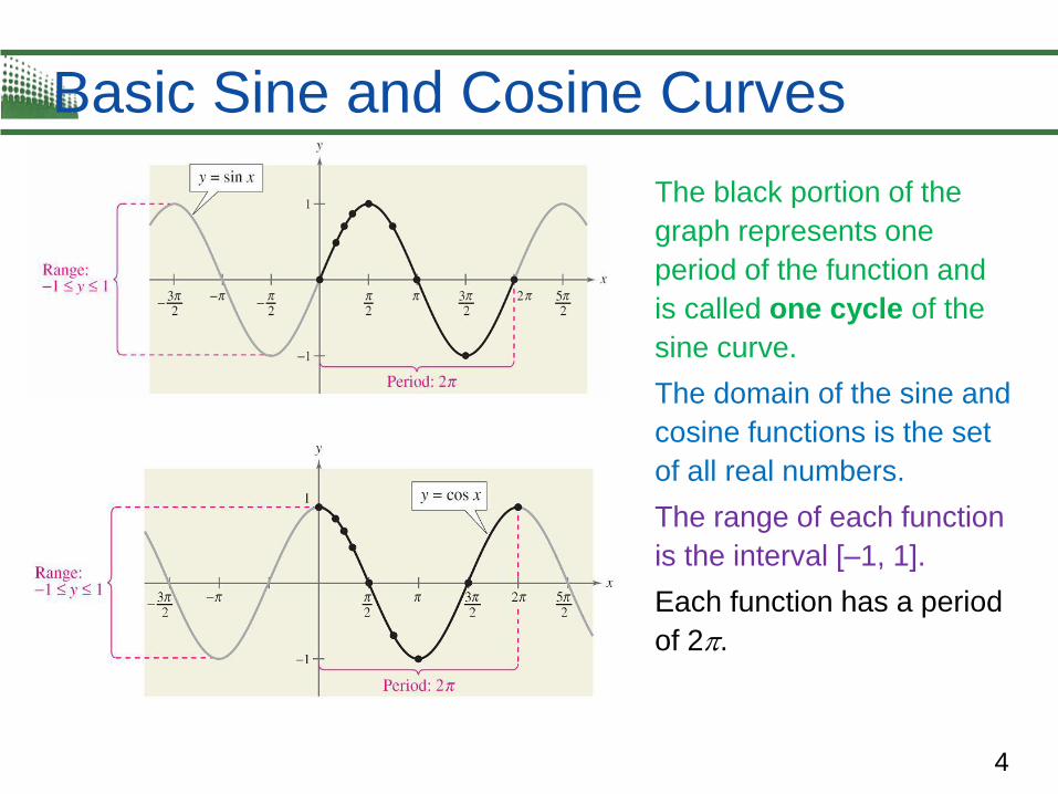
The black portion of the
graph represents one
period of the function and
is called one cycle of the
sine curve.
The domain of the sine and
cosine functions is the set
of all real numbers.
The range of each function
is the interval [–1, 1].
Each function has a period
of 2.
5
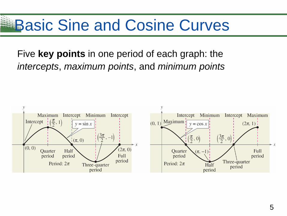
Basic Sine and Cosine Curves
Five key points in one period of each graph: the
intercepts, maximum points, and minimum points
6
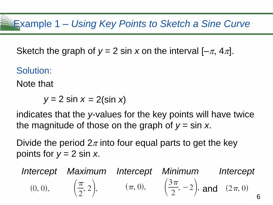
Example 1 – Using Key Points to Sketch a Sine Curve
Sketch the graph of y = 2 sin x on the interval [–, 4].
Solution:
Note that
y = 2 sin x
indicates that the y-values for the key points will have twice
the magnitude of those on the graph of y = sin x.
Divide the period 2 into four equal parts to get the key
points for y = 2 sin x.
Intercept Maximum Intercept Minimum Intercept
and
= 2(sin x)
7
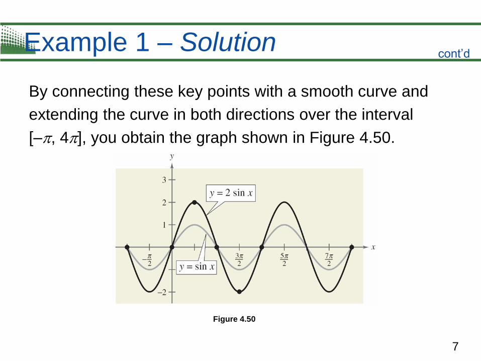
Example 1 – Solution
By connecting these key points with a smooth curve and
extending the curve in both directions over the interval
[–, 4], you obtain the graph shown in Figure 4.50.
cont’d
Figure 4.50
8
Amplitude and Period
9
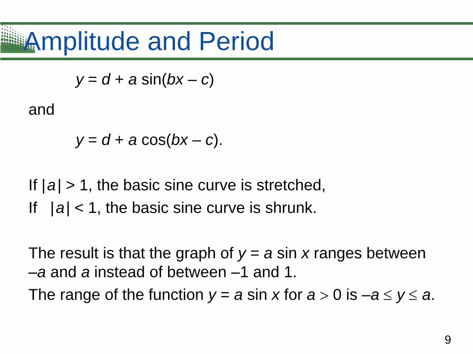
Amplitude and Period
y = d + a sin(bx – c)
and
y = d + a cos(bx – c).
If | a | > 1, the basic sine curve is stretched,
If | a | < 1, the basic sine curve is shrunk.
The result is that the graph of y = a sin x ranges between
–a and a instead of between –1 and 1.
The range of the function y = a sin x for a 0 is –a y a.
10
Amplitude and Period
11
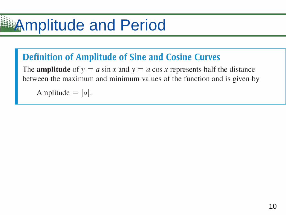
Amplitude and Period
12
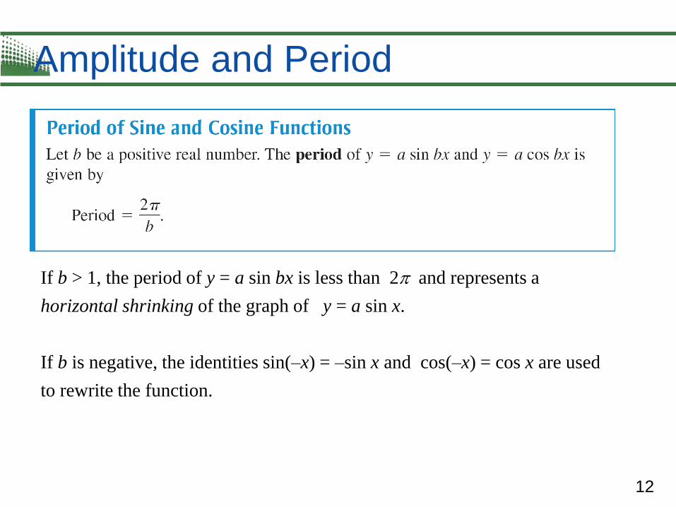
Amplitude and Period
If b > 1, the period of y = a sin bx is less than 2 and represents a
horizontal shrinking of the graph of y = a sin x.
If b is negative, the identities sin(–x) = –sin x and cos(–x) = cos x are used
to rewrite the function.
13
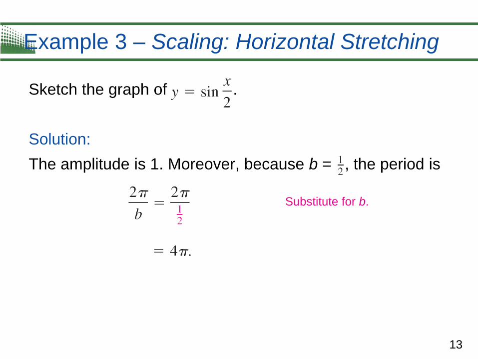
Example 3 – Scaling: Horizontal Stretching
Sketch the graph of .
Solution:
The amplitude is 1. Moreover, because b = , the period is
Substitute for b.
14
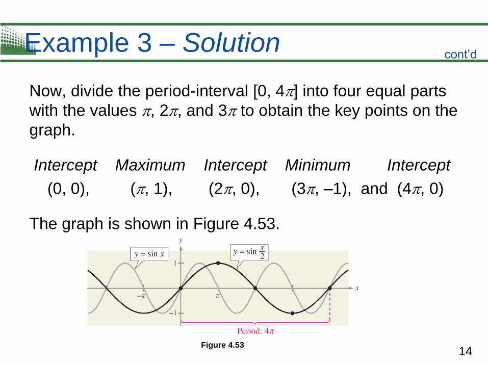
Example 3 – Solution
Now, divide the period-interval [0, 4] into four equal parts
with the values , 2, and 3 to obtain the key points on the
graph.
Intercept Maximum Intercept Minimum Intercept
(0, 0), (, 1), (2, 0), (3, –1), and (4, 0)
The graph is shown in Figure 4.53.
Figure 4.53
cont’d
15
Translations of Sine and Cosine
Curves
16
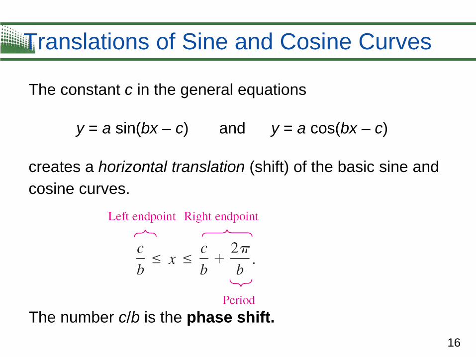
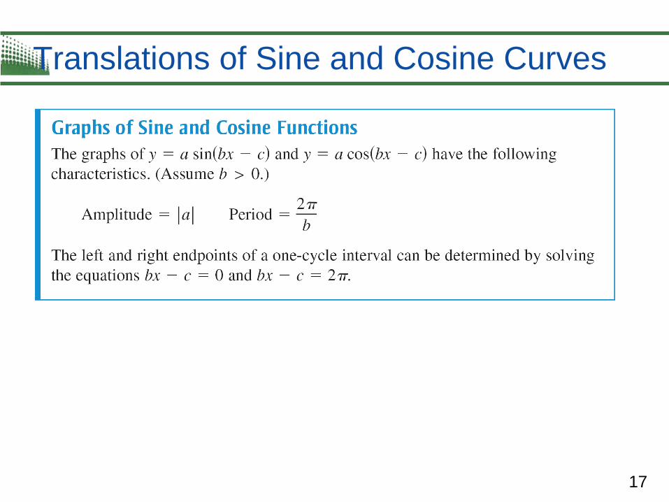
Translations of Sine and Cosine Curves
The constant c in the general equations
y = a sin(bx – c) and y = a cos(bx – c)
creates a horizontal translation (shift) of the basic sine and
cosine curves.
The number c/b is the phase shift.
17
Translations of Sine and Cosine Curves
18
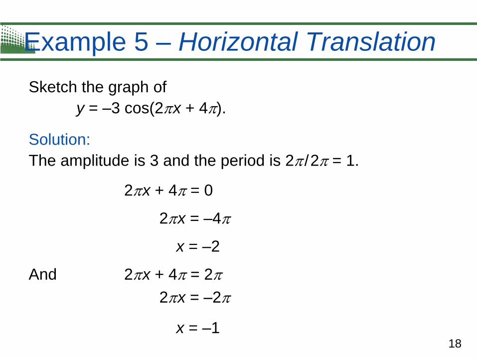
Example 5 – Horizontal Translation
Sketch the graph of
y = –3 cos(2 x + 4).
Solution:
The amplitude is 3 and the period is 2 / 2 = 1.
2 x + 4 = 0
2 x = –4
x = –2
And 2 x + 4 = 2
2 x = –2
x = –1
19
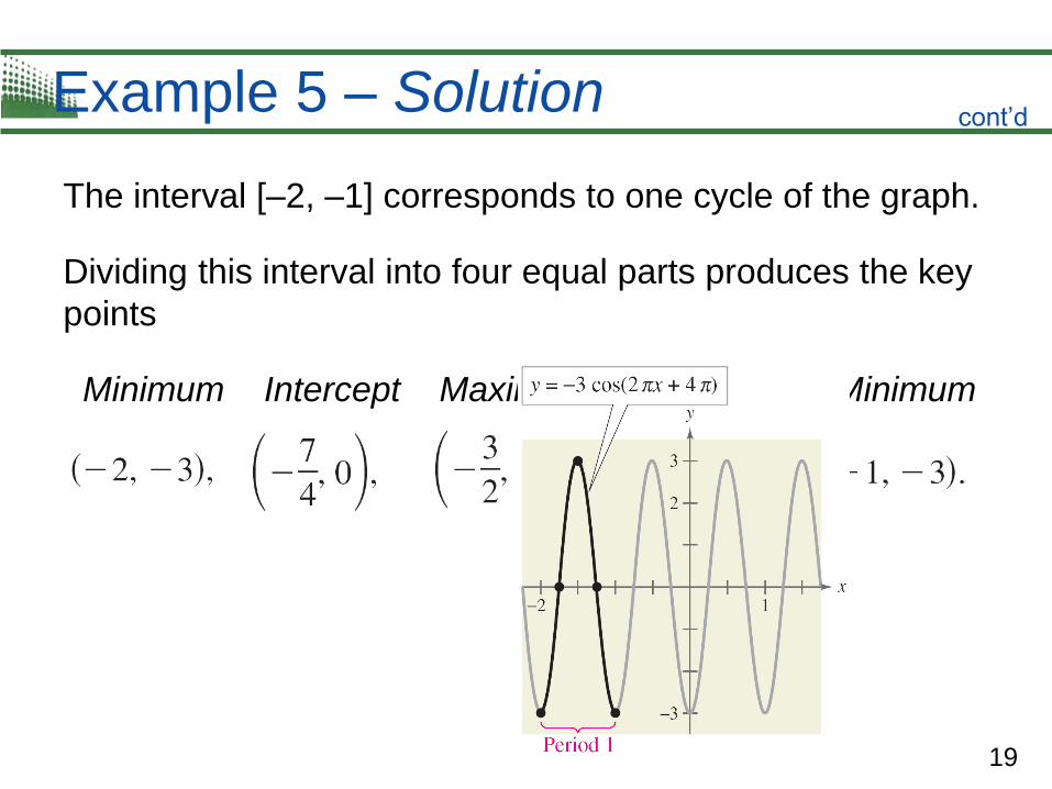
Example 5 – Solution
The interval [–2, –1] corresponds to one cycle of the graph.
Dividing this interval into four equal parts produces the key
points
Minimum Intercept Maximum Intercept Minimum
cont’d
20
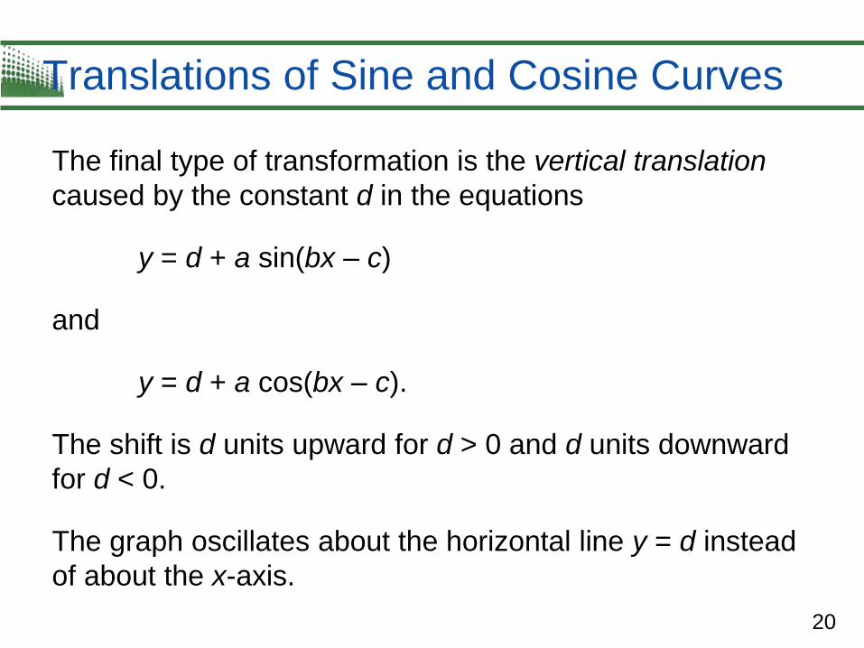
Translations of Sine and Cosine Curves
The final type of transformation is the vertical translation
caused by the constant d in the equations
y = d + a sin(bx – c)
and
y = d + a cos(bx – c).
The shift is d units upward for d > 0 and d units downward
for d < 0.
The graph oscillates about the horizontal line y = d instead
of about the x-axis.
21
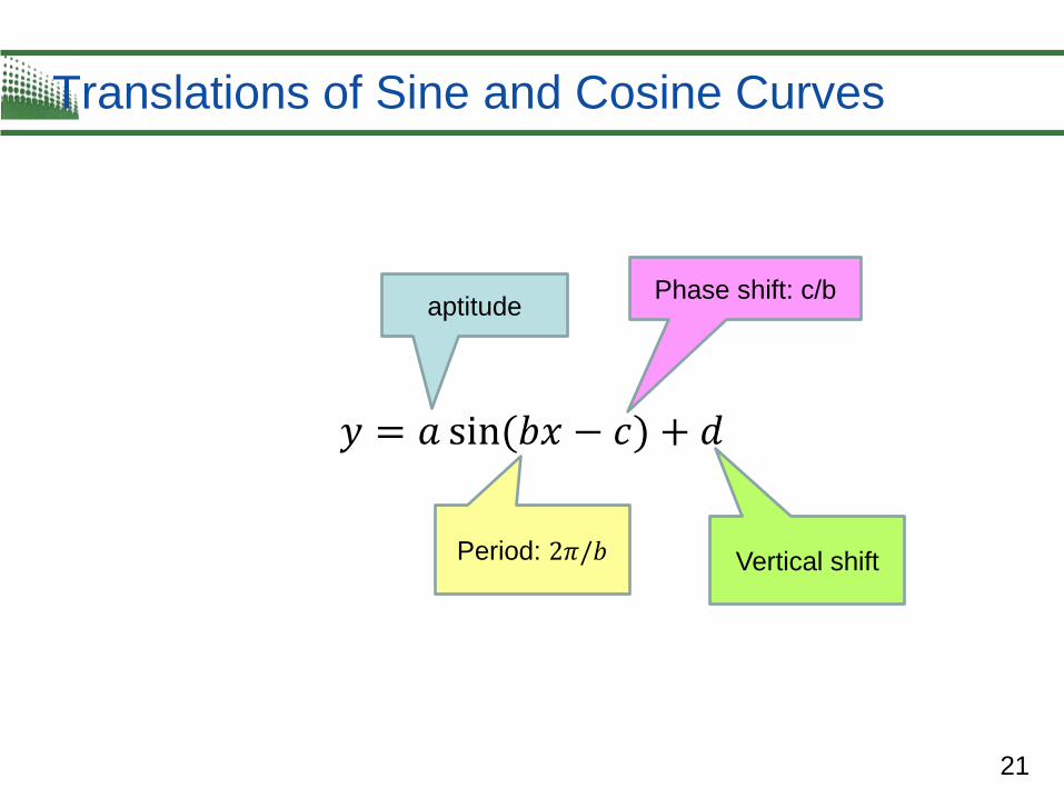
Translations of Sine and Cosine Curves
𝑦 = 𝑎 sin(𝑏𝑥 − 𝑐) + 𝑑
aptitude
Period: 2𝜋/𝑏 Vertical shift
Phase shift: c/b
22
Mathematical Modeling
23
Mathematical Modeling
Sine and cosine functions can be used to model many
real-life situations, including electric currents, musical tones,
radio waves, tides, and weather patterns.
24
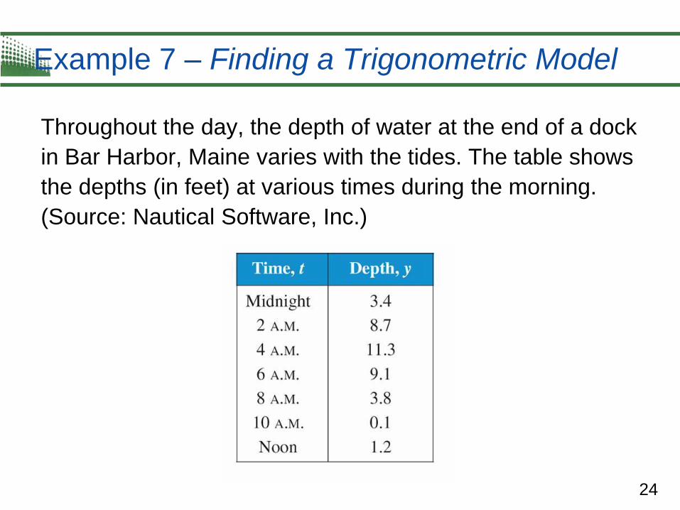
Example 7 – Finding a Trigonometric Model
Throughout the day, the depth of water at the end of a dock
in Bar Harbor, Maine varies with the tides. The table shows
the depths (in feet) at various times during the morning.
(Source: Nautical Software, Inc.)
25
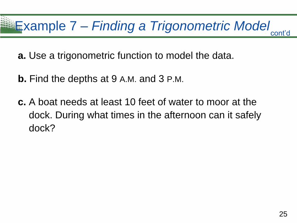
Example 7 – Finding a Trigonometric Model
a. Use a trigonometric function to model the data.
b. Find the depths at 9 A.M. and 3 P.M.
c. A boat needs at least 10 feet of water to moor at the
dock. During what times in the afternoon can it safely
dock?
cont’d

26
Example 7(a) – Solution
Begin by graphing the data, as shown in Figure 4.57.
You can use either a sine or a cosine model. Suppose you
use a cosine model of the form
y = a cos(bt – c) + d.
Changing Tides
Figure 4.57
27
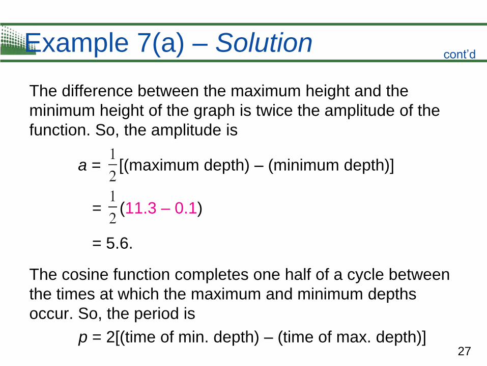
Example 7(a) – Solution
The difference between the maximum height and the
minimum height of the graph is twice the amplitude of the
function. So, the amplitude is
a = [(maximum depth) – (minimum depth)]
= (11.3 – 0.1)
= 5.6.
The cosine function completes one half of a cycle between
the times at which the maximum and minimum depths
occur. So, the period is
p = 2[(time of min. depth) – (time of max. depth)]
cont’d
28
Example 7(a) – Solution
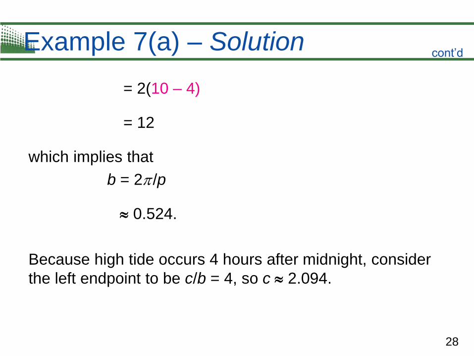
= 2(10 – 4)
= 12
which implies that
b = 2 /p
0.524.
Because high tide occurs 4 hours after midnight, consider
the left endpoint to be c/b = 4, so c 2.094.
cont’d
29
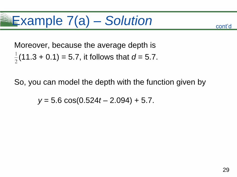
Example 7(a) – Solution
Moreover, because the average depth is
(11.3 + 0.1) = 5.7, it follows that d = 5.7.
So, you can model the depth with the function given by
y = 5.6 cos(0.524t – 2.094) + 5.7.
cont’d
30
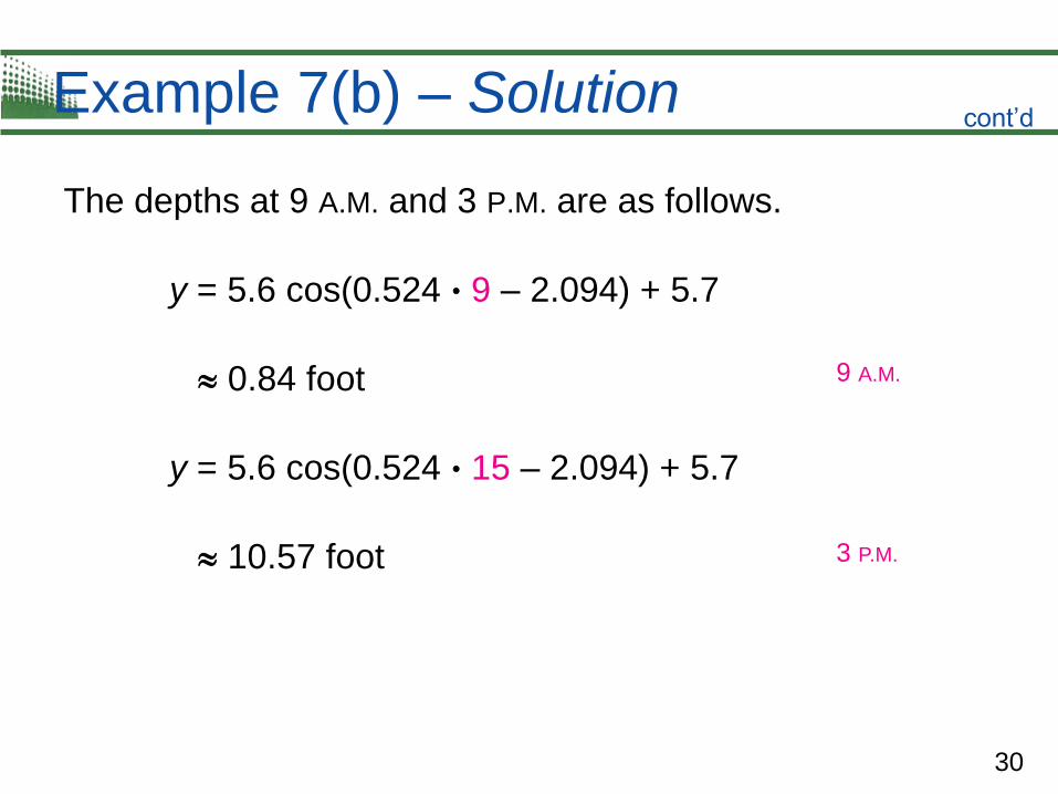
Example 7(b) – Solution
The depths at 9 A.M. and 3 P.M. are as follows.
y = 5.6 cos(0.524 9 – 2.094) + 5.7
0.84 foot
y = 5.6 cos(0.524 15 – 2.094) + 5.7
10.57 foot
9 A.M.
3 P.M.
cont’d
31
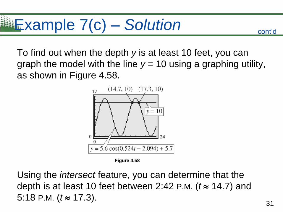
Example 7(c) – Solution
To find out when the depth y is at least 10 feet, you can
graph the model with the line y = 10 using a graphing utility,
as shown in Figure 4.58.
Using the intersect feature, you can determine that the
depth is at least 10 feet between 2:42 P.M. (t 14.7) and
5:18 P.M. (t 17.3).
Figure 4.58
cont’d