49

Fluid Mechanics Laboratory

Observation Note Book

By

Mr.B.Ramesh, M.E.,(Ph.D), Associate professor,

Department of Mechanical Engineering, St. Joseph’s College of Engineering,

Jeppiaar Trust, Chennai-119 Ph.D. Research Scholar, College of Engineering Guindy Campus, Anna

University, Chennai.

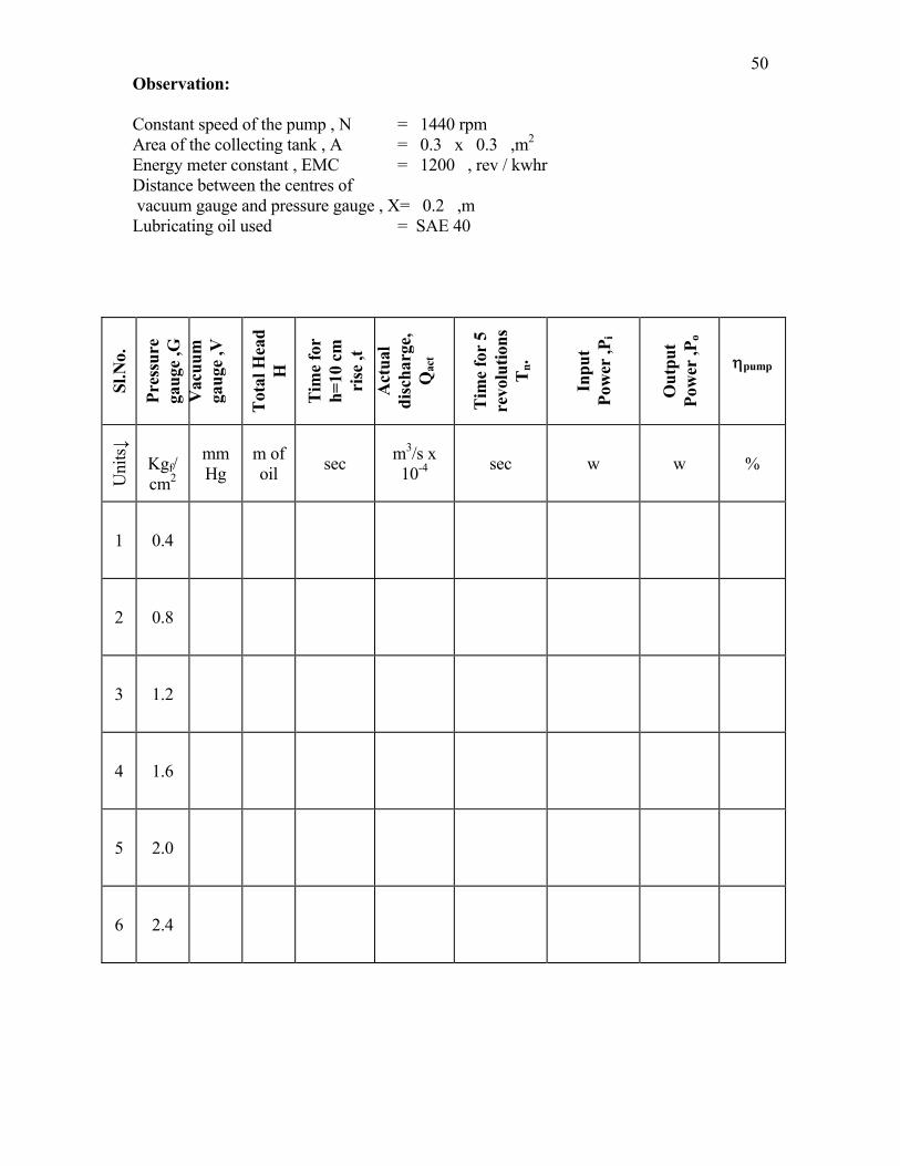
50Observation: Constant speed of the pump , N = 1440 rpm Area of the collecting tank , A = 0.3 x 0.3 ,m2 Energy meter constant , EMC = 1200 , rev / kwhr Distance between the centres of vacuum gauge and pressure gauge , X= 0.2 ,m Lubricating oil used = SAE 40

Sl.N

o.

Pres

sure

ga

uge

,G

Vac

uum

ga

uge

,V

Tot

al H

ead

H

Tim

e fo

r

h=10

cm

ri

se ,t

A

ctua

l di

scha

rge,

Q

act

Tim

e fo

r 5

revo

lutio

ns

T n.

Inpu

t Po

wer

,Pi

Out

put

Pow

er ,P

o

ηpump

Uni

ts↓

Kgf/ cm2

mmHg

m of oil sec m3/s x

10-4 sec w w %

1 0.4

2 0.8

3 1.2

4 1.6

5 2.0

6 2.4

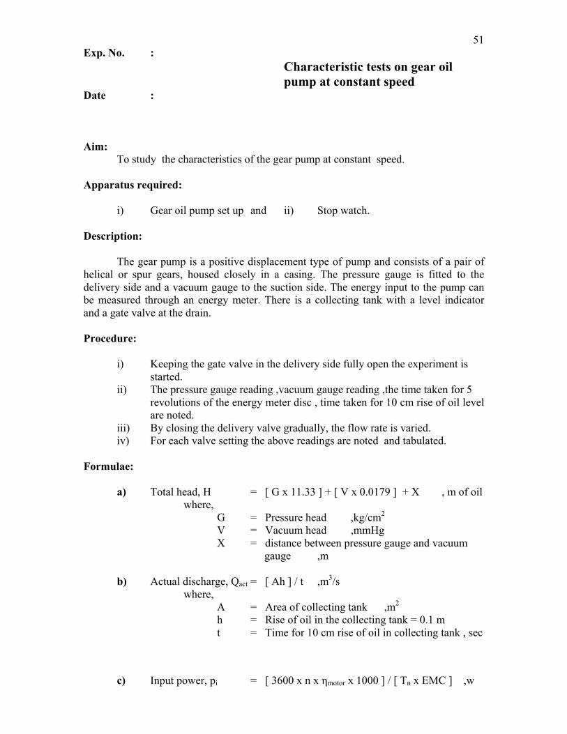
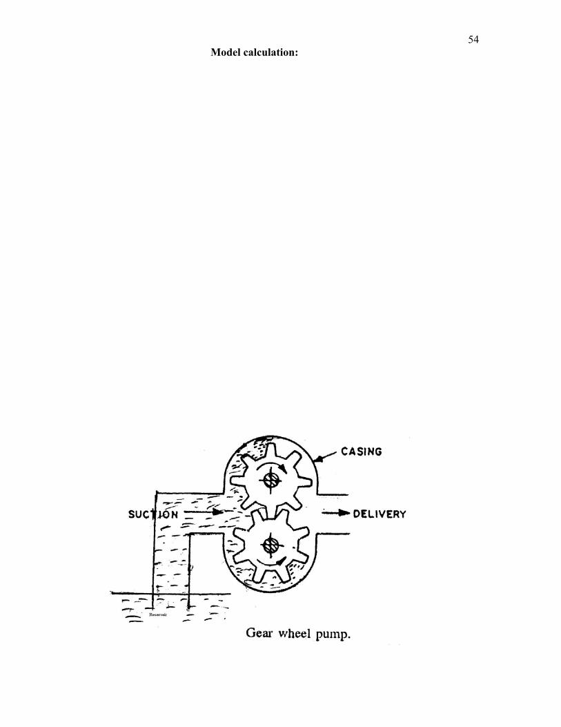
51Exp. No. : Characteristic tests on gear oil pump at constant speed Date : Aim: To study the characteristics of the gear pump at constant speed. Apparatus required: i) Gear oil pump set up and ii) Stop watch. Description: The gear pump is a positive displacement type of pump and consists of a pair of helical or spur gears, housed closely in a casing. The pressure gauge is fitted to the delivery side and a vacuum gauge to the suction side. The energy input to the pump can be measured through an energy meter. There is a collecting tank with a level indicator and a gate valve at the drain. Procedure: i) Keeping the gate valve in the delivery side fully open the experiment is started. ii) The pressure gauge reading ,vacuum gauge reading ,the time taken for 5 revolutions of the energy meter disc , time taken for 10 cm rise of oil level are noted. iii) By closing the delivery valve gradually, the flow rate is varied. iv) For each valve setting the above readings are noted and tabulated. Formulae: a) Total head, H = [ G x 11.33 ] + [ V x 0.0179 ] + X , m of oil where, G = Pressure head ,kg/cm2 V = Vacuum head ,mmHg X = distance between pressure gauge and vacuum gauge ,m b) Actual discharge, Qact = [ Ah ] / t ,m3/s where, A = Area of collecting tank ,m2

h = Rise of oil in the collecting tank = 0.1 m t = Time for 10 cm rise of oil in collecting tank , sec

c) Input power, pi = [ 3600 x n x ηmotor x 1000 ] / [ Tn x EMC ] ,w

52Model calculation:

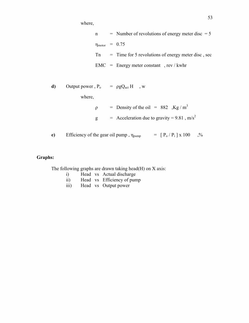
53 where,

n = Number of revolutions of energy meter disc = 5

ηmotor = 0.75

Tn = Time for 5 revolutions of energy meter disc , sec

EMC = Energy meter constant , rev / kwhr

d) Output power , Po = ρgQact H , w

where,

ρ = Density of the oil = 882 ,Kg / m3

g = Acceleration due to gravity = 9.81 , m/s2 e) Efficiency of the gear oil pump , ηpump = [ Po / Pi ] x 100 ,% Graphs: The following graphs are drawn taking head(H) on X axis: i) Head vs Actual discharge ii) Head vs Efficiency of pump iii) Head vs Output power

54Model calculation:

55

Result:

The characteristic test was conducted on the gear oil pump and the following graphs were drawn: i) H vs Qact ii) H vs ηpump and iii) H vs Po i) Maximum efficiency of gear oil pump, ηpump = ,%

ii) Actual discharge , Qact = ,m3/s

iii) Output power from the pump , Po = ,w

iv) Total head, H = ,m of oil

56 Observation:

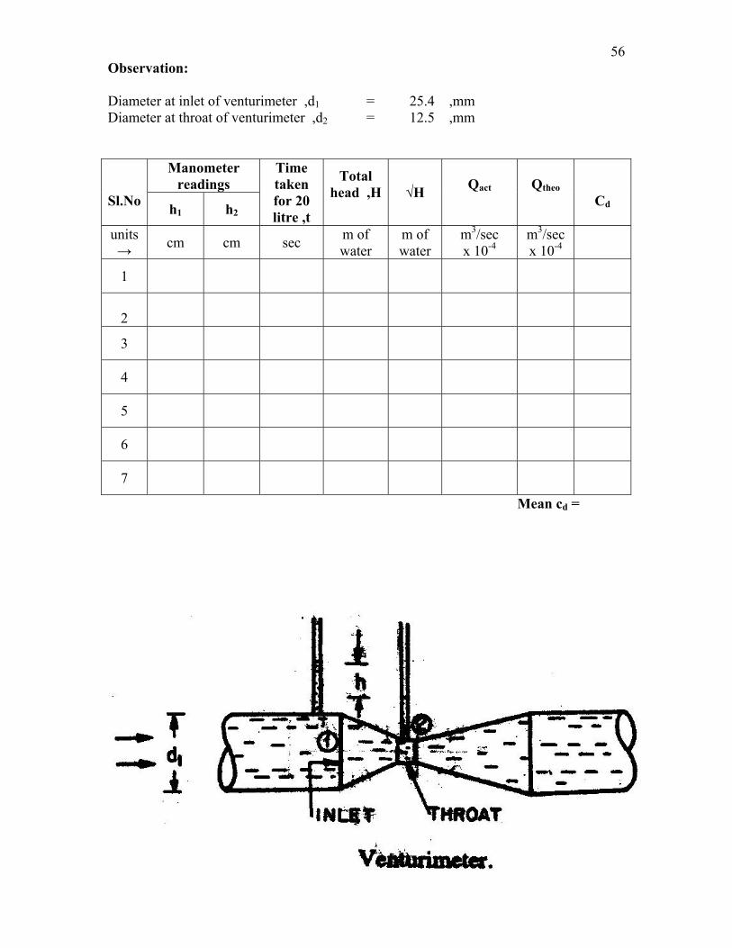
Diameter at inlet of venturimeter ,d1 = 25.4 ,mm Diameter at throat of venturimeter ,d2 = 12.5 ,mm

Sl.No

Manometer readings

Time taken for 20 litre ,t

Total head ,H

√H Qact

Qtheo

Cd h1 h2

units → cm cm sec m of

water m of water

m3/sec x 10-4

m3/sec x 10-4

1

2

3

4

5

6

7

Mean cd =

57Exp. No. : Venturimeter Date :

Aim: To find the co-efficient of discharge of the given venturimeter. Apparatus required: i) Venturimeter pipe set up ii) Mercury manometer and iii) Stop watch.

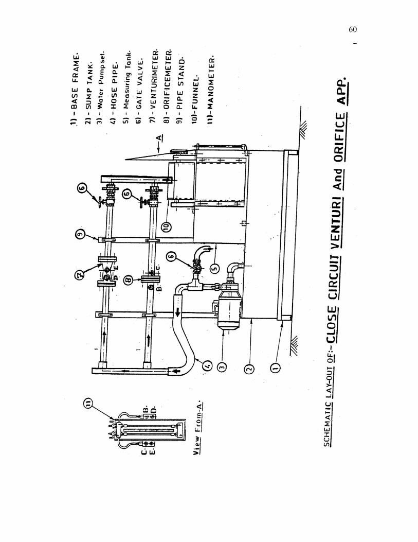
Description: i) The arrangement is of closed type. ii) Water is circulated through the venturimeter from reservoir to collecting tank by means of a monoblock pump. iii) The collecting tank of the venturimeter is connected to a mercury manometer. Procedure: i) The pump is primed and started. ii) Keeping the gate valve fully open the experiment is started. iii) The manometer readings and the time taken for 20 litre of water are noted. iv) The gate valve is gradually closed; for each valve setting the readings are noted and the values are tabulated. Formulae: a) Co-efficient of discharge ,Cd = Qact /Qtheo

b) Actual discharge , Qact = Volume of water collected / time taken for collection of 20 litres of water , m3/sec. c) Theoretical discharge ,Qtheo = [ a1a2√2gH ] / [ √ a1

2- a22 ] , m3/sec.

where, a1 = cross sectional area of inlet = π d1

2/4 ,m2 a2 = cross sectional area of throat = π d2

2/4 ,m2 d1 = diameter at inlet of the venturimeter ,m d2 = diameter at throat of the venturimeter ,m g = acceleration due to gravity = 9.81 ,m/sec2. d) Total head ,H = [ (h1- h2) /100 ] × [ ( SH / SL ) – 1 ] ,m of water = [ (h1- h2) /100 ] × [ ( 13.6 / 1 ) – 1 ] ,m of water where, h1- h2 = difference of mercury level in the manometer. SH = specific gravity of mercury = 13.6 SL = specific gravity of water = 1

58Model calculation:

59

60

61Graphs: The following graph is drawn: i) Qact vs Qtheo

Result : The co-efficient of discharge( cd ) of the given venturimeter is : i) Experimentally = ii) Graphically =

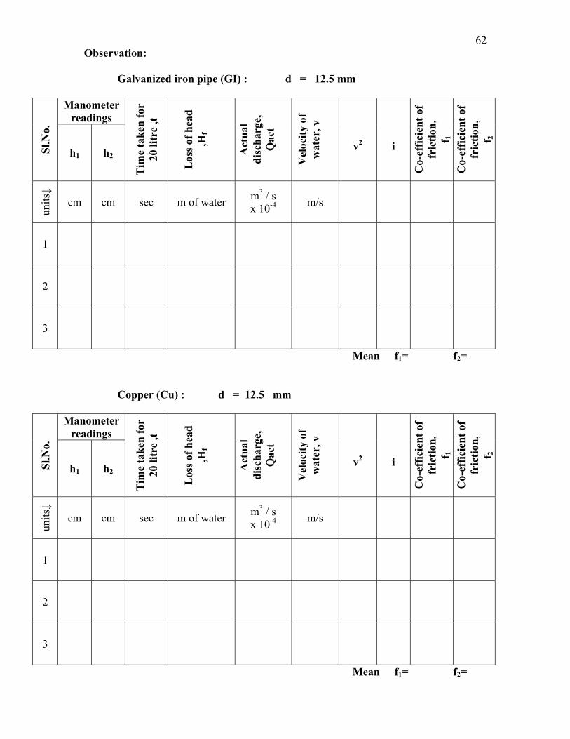
62 Observation: Galvanized iron pipe (GI) : d = 12.5 mm

Sl.N

o.

Manometer readings

Tim

e ta

ken

for

20 li

tre

,t

Los

s of h

ead

,Hf

Act

ual

disc

harg

e,

Qac

t

Vel

ocity

of

wat

er, v

v2 i

Co-

effic

ient

of

fric

tion,

f 1

C

o-ef

ficie

nt o

f fr

ictio

n,

f 2

h1 h2

units↓

cm cm sec m of water m3 / s x 10-4 m/s

1

2

3

Mean f1= f2= Copper (Cu) : d = 12.5 mm

Sl.N

o.

Manometer readings

Tim

e ta

ken

for

20 li

tre

,t

Los

s of h

ead

,Hf

Act

ual

disc

harg

e,

Qac

t

Vel

ocity

of

wat

er, v

v2 i

Co-

effic

ient

of

fric

tion,

f 1

C

o-ef

ficie

nt o

f fr

ictio

n,

f 2

h1 h2

units↓

cm cm sec m of water m3 / s x 10-4 m/s

1

2

3

Mean f1= f2=

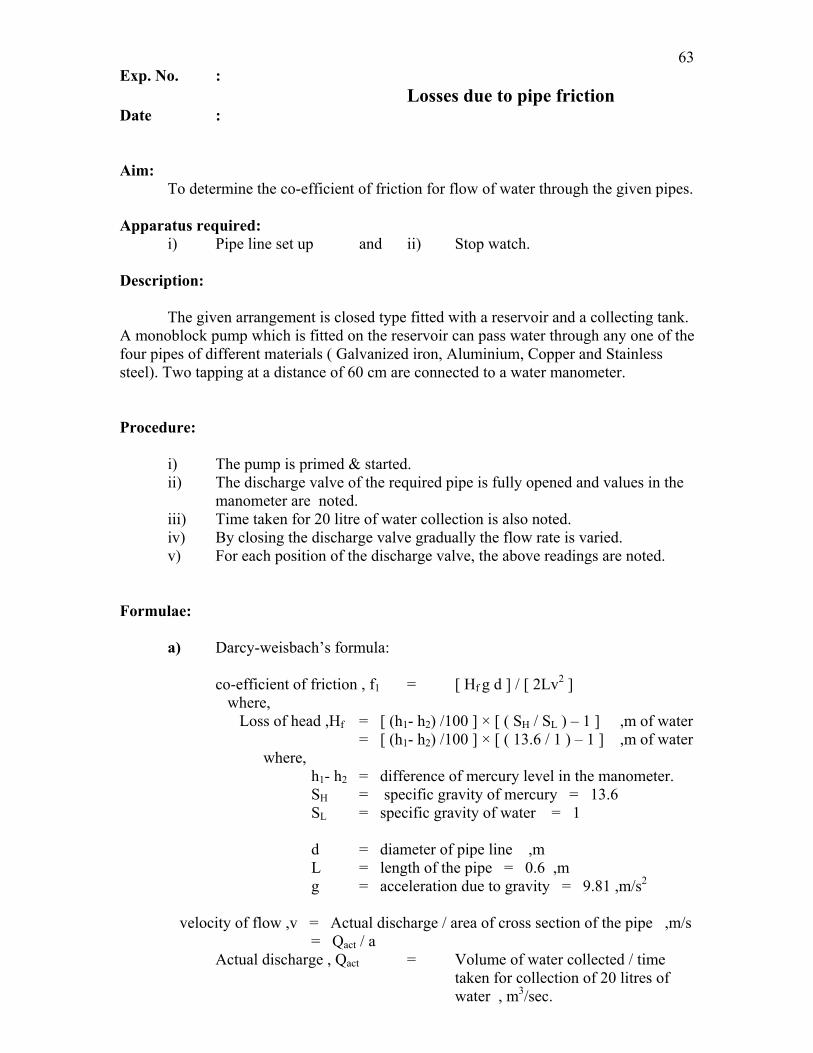
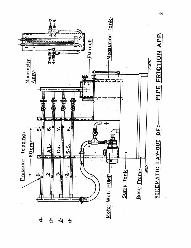
63Exp. No. : Losses due to pipe friction Date :

Aim: To determine the co-efficient of friction for flow of water through the given pipes. Apparatus required: i) Pipe line set up and ii) Stop watch. Description: The given arrangement is closed type fitted with a reservoir and a collecting tank. A monoblock pump which is fitted on the reservoir can pass water through any one of the four pipes of different materials ( Galvanized iron, Aluminium, Copper and Stainless steel). Two tapping at a distance of 60 cm are connected to a water manometer. Procedure: i) The pump is primed & started. ii) The discharge valve of the required pipe is fully opened and values in the manometer are noted. iii) Time taken for 20 litre of water collection is also noted. iv) By closing the discharge valve gradually the flow rate is varied. v) For each position of the discharge valve, the above readings are noted. Formulae: a) Darcy-weisbach’s formula: co-efficient of friction , f1 = [ Hf g d ] / [ 2Lv2 ] where,

Loss of head ,Hf = [ (h1- h2) /100 ] × [ ( SH / SL ) – 1 ] ,m of water = [ (h1- h2) /100 ] × [ ( 13.6 / 1 ) – 1 ] ,m of water where, h1- h2 = difference of mercury level in the manometer. SH = specific gravity of mercury = 13.6 SL = specific gravity of water = 1 d = diameter of pipe line ,m L = length of the pipe = 0.6 ,m g = acceleration due to gravity = 9.81 ,m/s2

velocity of flow ,v = Actual discharge / area of cross section of the pipe ,m/s = Qact / a

Actual discharge , Qact = Volume of water collected / time taken for collection of 20 litres of water , m3/sec.

64Model calculation:

65

66

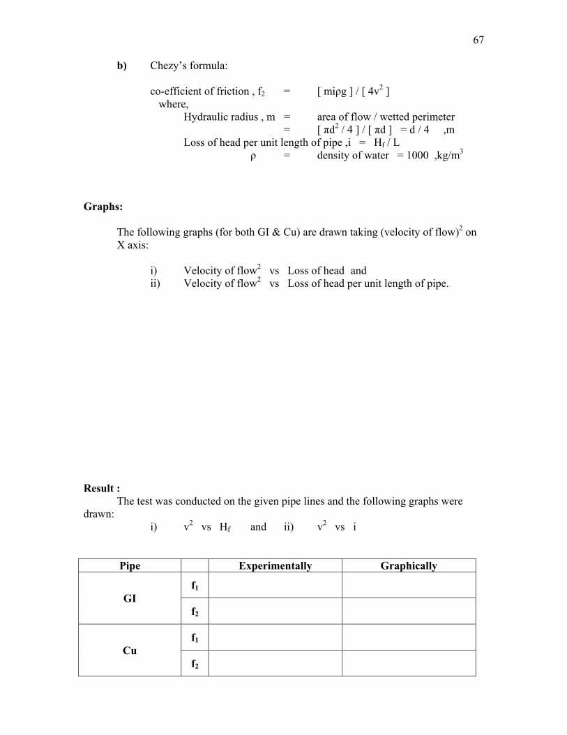
67 b) Chezy’s formula: co-efficient of friction , f2 = [ miρg ] / [ 4v2 ] where, Hydraulic radius , m = area of flow / wetted perimeter = [ πd2 / 4 ] / [ πd ] = d / 4 ,m Loss of head per unit length of pipe ,i = Hf / L ρ = density of water = 1000 ,kg/m3 Graphs: The following graphs (for both GI & Cu) are drawn taking (velocity of flow)2 on X axis: i) Velocity of flow2 vs Loss of head and ii) Velocity of flow2 vs Loss of head per unit length of pipe. Result : The test was conducted on the given pipe lines and the following graphs were drawn: i) v2 vs Hf and ii) v2 vs i

Pipe Experimentally Graphically

GI f1

f2

Cu f1

f2

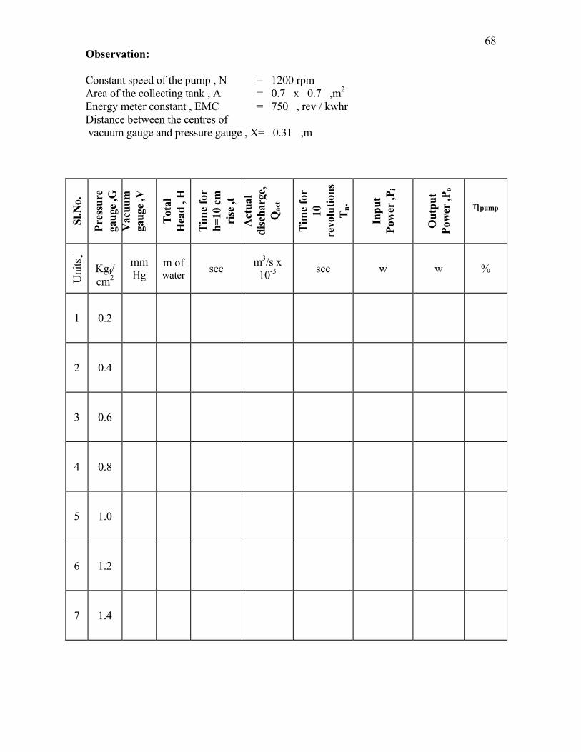
68Observation: Constant speed of the pump , N = 1200 rpm Area of the collecting tank , A = 0.7 x 0.7 ,m2 Energy meter constant , EMC = 750 , rev / kwhr Distance between the centres of vacuum gauge and pressure gauge , X= 0.31 ,m

Sl.N

o.

Pres

sure

ga

uge

,G

Vac

uum

ga

uge

,V

Tot

al

Hea

d , H

Tim

e fo

r

h=10

cm

ri

se ,t

A

ctua

l di

scha

rge,

Q

act

Tim

e fo

r 10

re

volu

tions

T n

.

Inpu

t Po

wer

,Pi

Out

put

Pow

er ,P

o

ηpump

Uni

ts↓

Kgf/ cm2

mmHg

m of water sec m3/s x

10-3 sec w w %

1 0.2

2 0.4

3 0.6

4 0.8

5 1.0

6 1.2

7 1.4

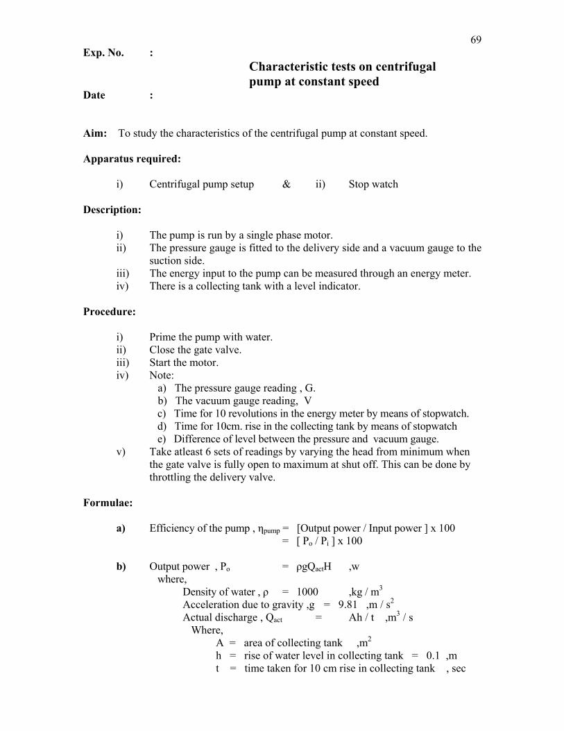
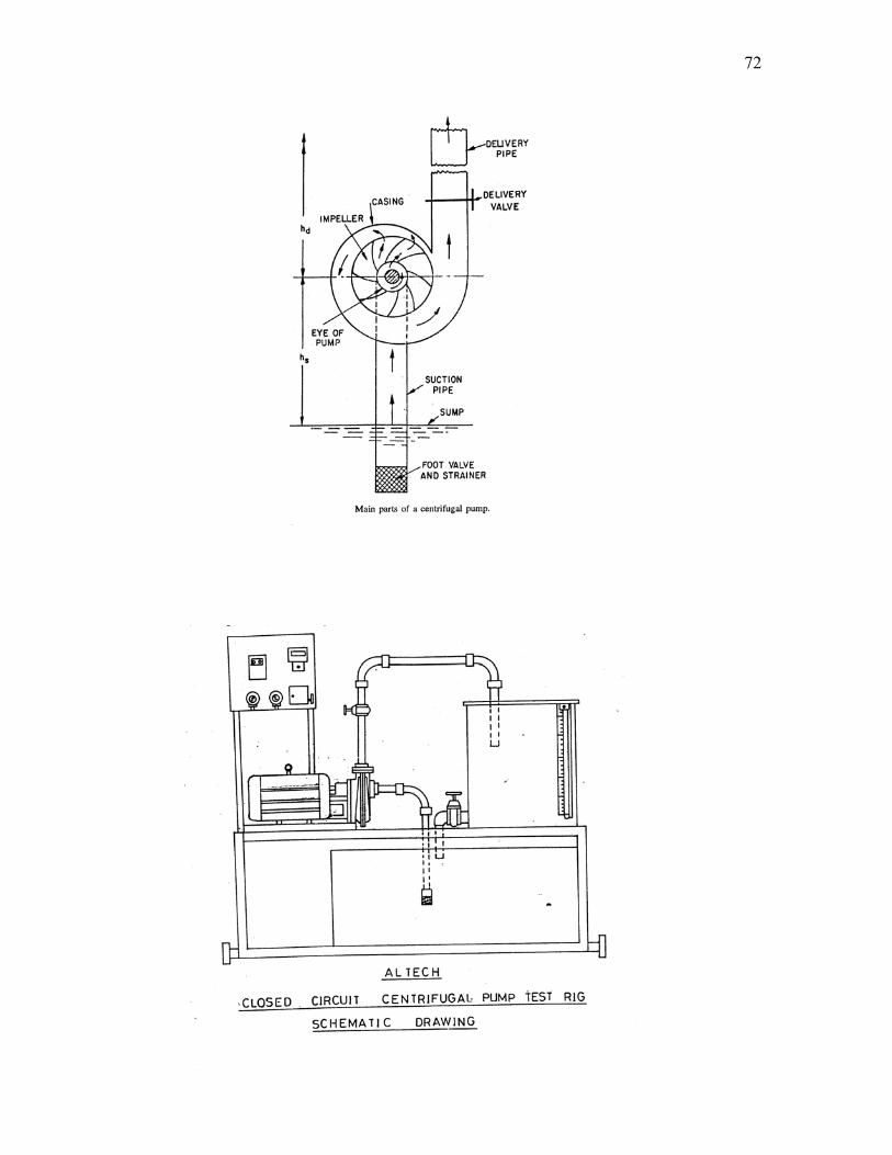
69Exp. No. : Characteristic tests on centrifugal pump at constant speed Date : Aim: To study the characteristics of the centrifugal pump at constant speed. Apparatus required: i) Centrifugal pump setup & ii) Stop watch Description: i) The pump is run by a single phase motor.

ii) The pressure gauge is fitted to the delivery side and a vacuum gauge to the suction side. iii) The energy input to the pump can be measured through an energy meter. iv) There is a collecting tank with a level indicator.

Procedure: i) Prime the pump with water. ii) Close the gate valve. iii) Start the motor. iv) Note: a) The pressure gauge reading , G. b) The vacuum gauge reading, V c) Time for 10 revolutions in the energy meter by means of stopwatch. d) Time for 10cm. rise in the collecting tank by means of stopwatch e) Difference of level between the pressure and vacuum gauge. v) Take atleast 6 sets of readings by varying the head from minimum when the gate valve is fully open to maximum at shut off. This can be done by throttling the delivery valve. Formulae: a) Efficiency of the pump , ηpump = [Output power / Input power ] x 100 = [ Po / Pi ] x 100 b) Output power , Po = ρgQactH ,w where, Density of water , ρ = 1000 ,kg / m3 Acceleration due to gravity ,g = 9.81 ,m / s2 Actual discharge , Qact = Ah / t ,m3 / s Where, A = area of collecting tank ,m2 h = rise of water level in collecting tank = 0.1 ,m t = time taken for 10 cm rise in collecting tank , sec

70Model calculation:

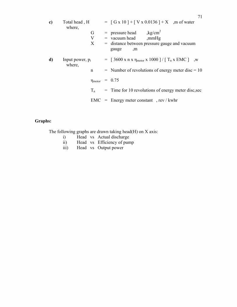
71 c) Total head , H = [ G x 10 ] + [ V x 0.0136 ] + X ,m of water where, G = pressure head ,kg/cm2 V = vacuum head ,mmHg X = distance between pressure gauge and vacuum gauge ,m d) Input power, pi = [ 3600 x n x ηmotor x 1000 ] / [ Tn x EMC ] ,w where, n = Number of revolutions of energy meter disc = 10

ηmotor = 0.75

Tn = Time for 10 revolutions of energy meter disc,sec

EMC = Energy meter constant , rev / kwhr

Graphs: The following graphs are drawn taking head(H) on X axis: i) Head vs Actual discharge ii) Head vs Efficiency of pump iii) Head vs Output power

72

73

Result:

The characteristic test was conducted on the centrifugal pump and the following graphs were drawn: i) H vs Qact ii) H vs ηpump and iii) H vs Po i) Maximum efficiency of centrifugal pump, ηpump = ,%

ii) Actual discharge , Qact = ,m3/s

iii) Output power from the pump , Po = ,w

iv) Total head, H = ,m of water

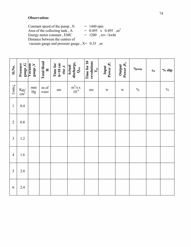
74Observation: Constant speed of the pump , N = 1440 rpm Area of the collecting tank , A = 0.495 x 0.495 ,m2 Energy meter constant , EMC = 1200 , rev / kwhr Distance between the centres of vacuum gauge and pressure gauge , X= 0.35 ,m

Sl.N

o.

Pres

sure

ga

uge

,G

Vac

uum

ga

uge

,V

Tot

al H

ead

H

Tim

e fo

r

h=10

cm

ri

se ,t

A

ctua

l di

scha

rge,

Q

act

Tim

e fo

r 10

re

volu

tions

T n

.

Inpu

t Po

wer

,Pi

Out

put

Pow

er ,P

o

ηpump cd % slip

Uni

ts↓

Kgf/ cm2

mmHg

m of water sec m3/s x

10-4 sec w w %

%

1 0.4

2 0.8

3 1.2

4 1.6

5 2.0

6 2.4

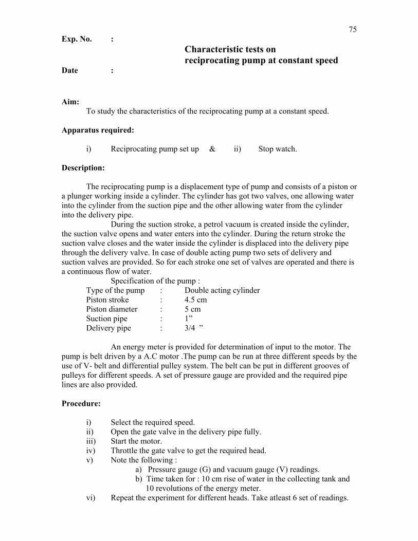
75Exp. No. : Characteristic tests on reciprocating pump at constant speed Date :

Aim: To study the characteristics of the reciprocating pump at a constant speed. Apparatus required: i) Reciprocating pump set up & ii) Stop watch.

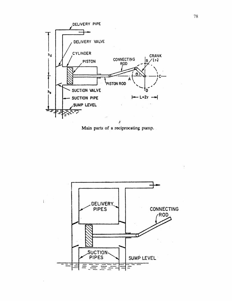
Description: The reciprocating pump is a displacement type of pump and consists of a piston or

a plunger working inside a cylinder. The cylinder has got two valves, one allowing water into the cylinder from the suction pipe and the other allowing water from the cylinder into the delivery pipe. During the suction stroke, a petrol vacuum is created inside the cylinder, the suction valve opens and water enters into the cylinder. During the return stroke the suction valve closes and the water inside the cylinder is displaced into the delivery pipe through the delivery valve. In case of double acting pump two sets of delivery and suction valves are provided. So for each stroke one set of valves are operated and there is a continuous flow of water. Specification of the pump : Type of the pump : Double acting cylinder

Piston stroke : 4.5 cm Piston diameter : 5 cm Suction pipe : 1” Delivery pipe : 3/4 ” An energy meter is provided for determination of input to the motor. The

pump is belt driven by a A.C motor .The pump can be run at three different speeds by the use of V- belt and differential pulley system. The belt can be put in different grooves of pulleys for different speeds. A set of pressure gauge are provided and the required pipe lines are also provided. Procedure: i) Select the required speed. ii) Open the gate valve in the delivery pipe fully. iii) Start the motor. iv) Throttle the gate valve to get the required head. v) Note the following : a) Pressure gauge (G) and vacuum gauge (V) readings. b) Time taken for : 10 cm rise of water in the collecting tank and 10 revolutions of the energy meter. vi) Repeat the experiment for different heads. Take atleast 6 set of readings.

76Model calculation:

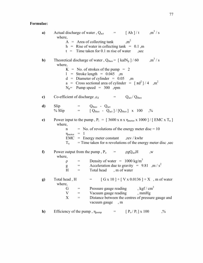
77 Formulae: a) Actual discharge of water , Qact = [ Ah ] / t ,m3 / s where, A = Area of collecting tank ,m2 h = Rise of water in collecting tank = 0.1 ,m t = Time taken for 0.1 m rise of water ,sec b) Theoretical discharge of water , Qtheo = [ kalNp ] / 60 ,m3 / s where, K = No. of strokes of the pump = 2 l = Stroke length = 0.045 ,m d = Diameter of cylinder = 0.05 ,m a = Cross sectional area of cylinder = [ πd2 ] / 4 ,m2 Np= Pump speed = 300 ,rpm c) Co-efficient of discharge ,cd = Qact / Qtheo d) Slip = Qtheo - Qact % Slip = [ Qtheo - Qact ] / [Qtheo ] x 100 ,% e) Power input to the pump , Pi = [ 3600 x n x ηmotor x 1000 ] / [ EMC x Tn ] where, n = No. of revolutions of the energy meter disc = 10 ηmotor = 1 EMC = Energy meter constant ,rev / kwhr Tn = Time taken for n revolutions of the energy meter disc ,sec f) Power output from the pump , Po = ρgQactH ,w where, ρ = Density of water = 1000 kg/m3 g = Acceleration due to gravity = 9.81 ,m / s2 H = Total head , m of water g) Total head , H = [ G x 10 ] + [ V x 0.0136 ] + X , m of water where, G = Pressure gauge reading , kgf / cm2 V = Vacuum gauge reading , mmHg X = Distance between the centres of pressure gauge and vacuum gauge , m h) Efficiency of the pump , ηpump = [ Po / Pi ] x 100 ,%

78

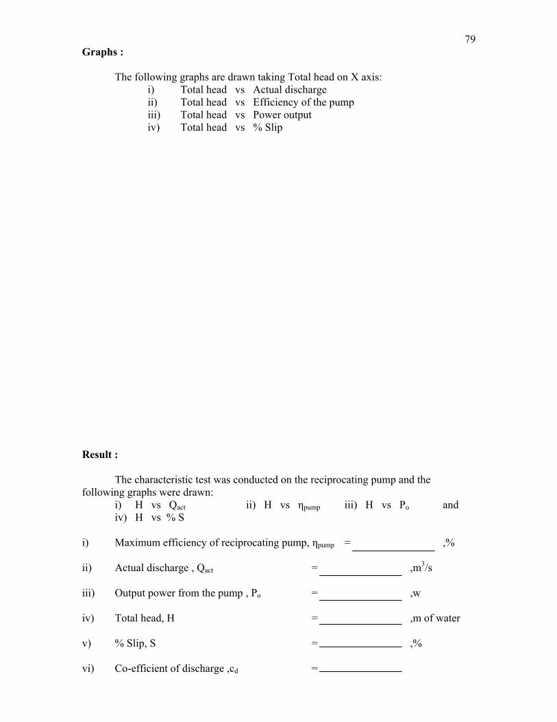
79Graphs : The following graphs are drawn taking Total head on X axis: i) Total head vs Actual discharge ii) Total head vs Efficiency of the pump iii) Total head vs Power output iv) Total head vs % Slip Result :

The characteristic test was conducted on the reciprocating pump and the following graphs were drawn: i) H vs Qact ii) H vs ηpump iii) H vs Po and iv) H vs % S i) Maximum efficiency of reciprocating pump, ηpump = ,%

ii) Actual discharge , Qact = ,m3/s

iii) Output power from the pump , Po = ,w

iv) Total head, H = ,m of water

v) % Slip, S = ,%

vi) Co-efficient of discharge ,cd =

80

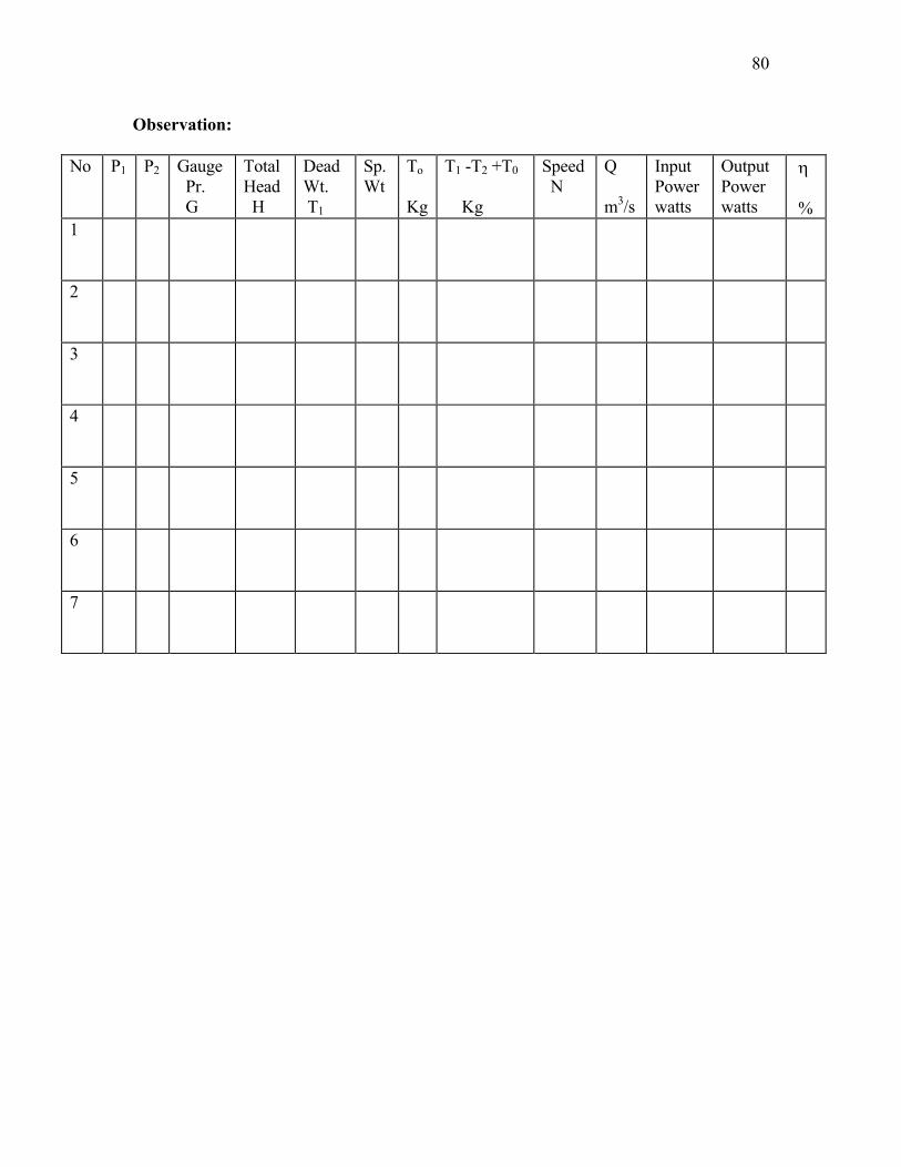
Observation:

No P1 P2 Gauge Pr. G

Total Head H

Dead Wt. T1

Sp. Wt

To Kg

T1 -T2 +T0 Kg

Speed N

Q m3/s

Input Power watts

Output Power watts

η %

1

2

3

4

5

6

7

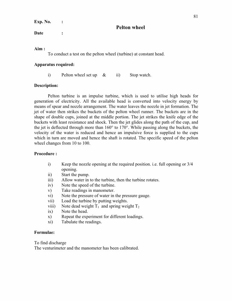
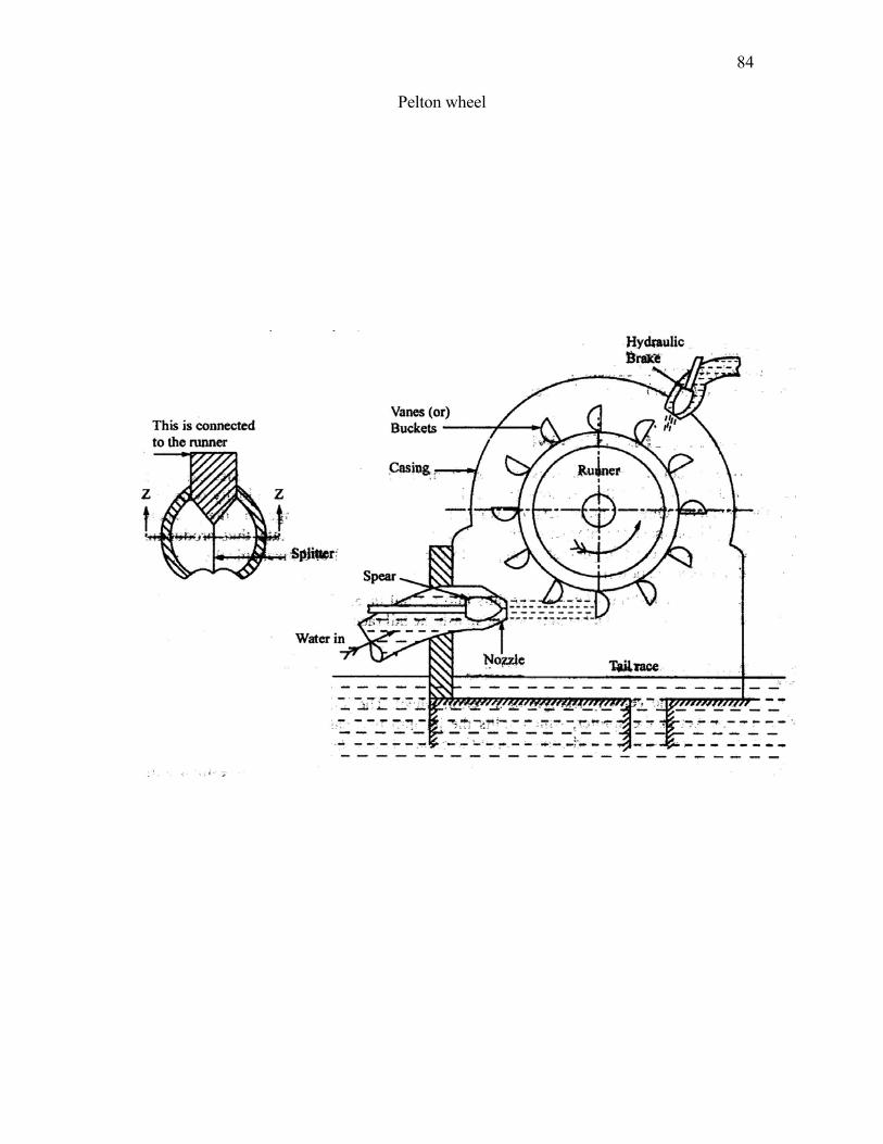
81Exp. No. : Pelton wheel Date : Aim : To conduct a test on the pelton wheel (turbine) at constant head. Apparatus required: i) Pelton wheel set up & ii) Stop watch. Description: Pelton turbine is an impulse turbine, which is used to utilise high heads for generation of electricity. All the available head is converted into velocity energy by means of spear and nozzle arrangement. The water leaves the nozzle in jet formation. The jet of water then strikes the buckets of the pelton wheel runner. The buckets are in the shape of double cups, joined at the middle portion. The jet strikes the knife edge of the buckets with least resistance and shock. Then the jet glides along the path of the cup, and the jet is deflected through more than 160° to 170°. While passing along the buckets, the velocity of the water is reduced and hence an impulsive force is supplied to the cups which in turn are moved and hence the shaft is rotated. The specific speed of the pelton wheel changes from 10 to 100. Procedure : i) Keep the nozzle opening at the required position. i.e. full opening or 3/4 opening. ii) Start the pump. iii) Allow water in to the turbine, then the turbine rotates. iv) Note the speed of the turbine. v) Take readings in manometer. vi) Note the pressure of water in the pressure gauge. vii) Load the turbine by putting weights. viii) Note dead weight T1 and spring weight T2 ix) Note the head. x) Repeat the experiment for different loadings. xi) Tabulate the readings. Formulae: To find discharge The venturimeter and the manometer has been calibrated.

82Model calculation:

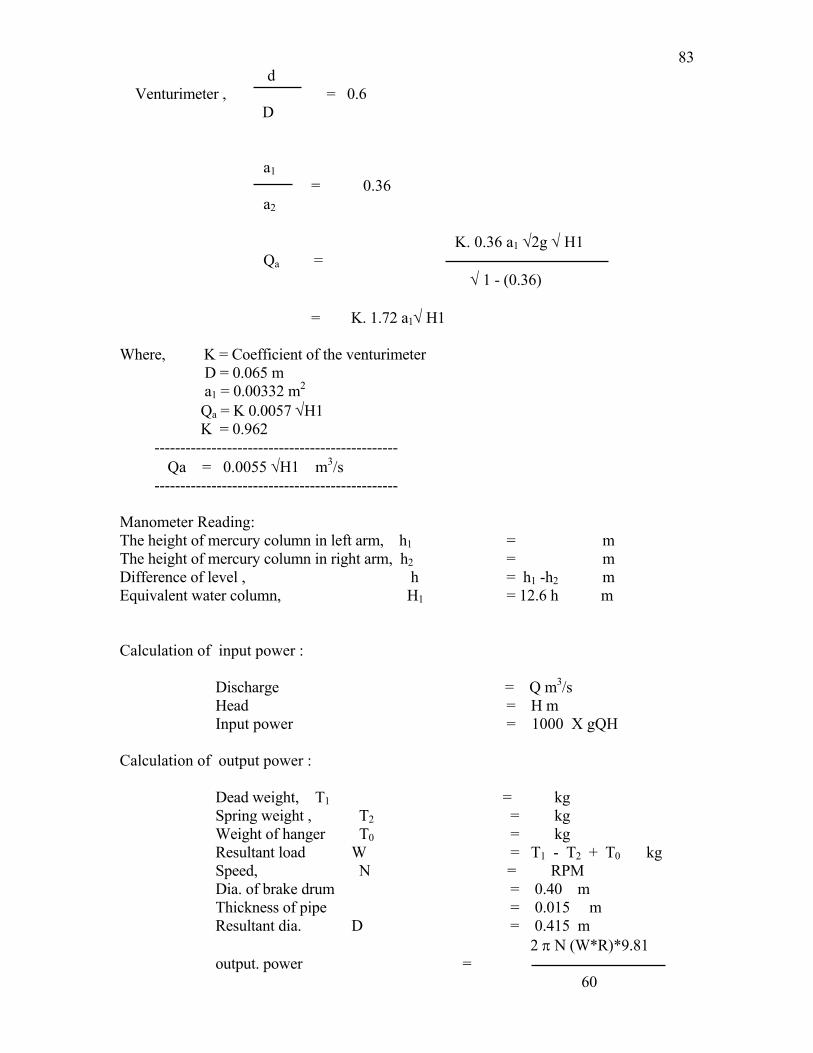
83 d Venturimeter , = 0.6 D a1 = 0.36 a2 K. 0.36 a1 √2g √ H1 Qa = √ 1 - (0.36) = K. 1.72 a1√ H1 Where, K = Coefficient of the venturimeter D = 0.065 m a1 = 0.00332 m2 Qa = K 0.0057 √H1 K = 0.962 ----------------------------------------------- Qa = 0.0055 √H1 m3/s ----------------------------------------------- Manometer Reading: The height of mercury column in left arm, h1 = m The height of mercury column in right arm, h2 = m Difference of level , h = h1 -h2 m Equivalent water column, H1 = 12.6 h m Calculation of input power : Discharge = Q m3/s Head = H m Input power = 1000 X gQH Calculation of output power : Dead weight, T1 = kg Spring weight , T2 = kg Weight of hanger T0 = kg Resultant load W = T1 - T2 + T0 kg Speed, N = RPM Dia. of brake drum = 0.40 m Thickness of pipe = 0.015 m Resultant dia. D = 0.415 m 2 π N (W*R)*9.81 output. power = 60

84

Pelton wheel

85 Result: A test is conducted on Pelton wheel (turbine) and the following graphs were drawn. i) Output power Vs N & ii) Efficiency Vs N

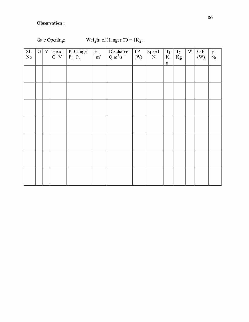
86Observation : Gate Opening: Weight of Hanger T0 = 1Kg.

Sl.No

G V

Head G+V

Pr.Gauge P1 P2

H1 `m’

Discharge Q m3/s

I P (W)

Speed N

T1 Kg

T2 Kg

W O P (W)

η %

87Exp. No. : Francis turbine Date :

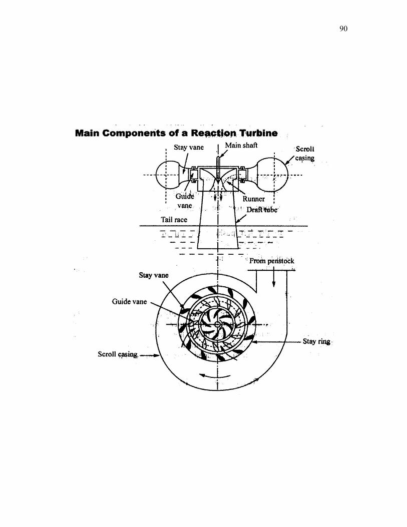
Aim: To study the characteristics of Francis Turbine at constant head. Apparatus required: i) Francis turbine set up & ii) Stop watch. Description: Francis turbine is a prime mover. It converts the hydraulic energy (head of water) into mechanical energy, which in turn can be transformed into electrical energy by coupling a generator to the turbine. Francis Turbine is a radial inward flow reaction turbine. This has the advantage of centrifugal force acting against the flow, thus reducing the tendency of the wheel to race. The turbine consists essentially of runner (G.M.), a ring of adjustable guide vanes, a volute casing(spiral casing) , draft tube. Francis turbines are best suited for medium heads, say 40m to 300m. The specific speed ranges from 25 to 300. Procedure: i) Keep the guide vanes fully opened or 6/8 opening. ii) Prime the pump iii) Start the pump iv) Vent the manometer v) Note the pressure gauge reading (G) and vacuum gauge reading (V). vi) Adjust the gate valve so that G +V reads = 15m. vii) Note the readings in the pressure gauge Left limb reading = P1 m Right limb reading = P2 m. viii) Measure the speed of the turbine by tachometer ix) Load the turbine by putting weights in the weights hanger. Take all readings. x) Repeat the experiments for various loadings and take 6 readings. xi) Experiment can be repeated for different guide vane opening. Formulae: I. Discharge: Pressure gauge readings: Left limb reading = P1m. Right limb reading = P2m. Difference of levels H1 = (P1 -P2) 10 m of water

88Model calculation:

89Venturimeter equation Q = 0.0131 ÖH1 m3/s II. Head: Pressure gauge = G m. Vaccuum gauge = V m. Total Head = G + V + X ,(X = Difference of levels pressure & vacuum gauge) = H m. III. Input to the turbine: I. H. P. = 1000 QH 75 IV. Output: Brake drum diameter = 0.30m. Rope diameter = 0.015m Equivalent drum diameter = 0.315m. Hanger weight = T0 Kg = 1 kg. Dead Weight = T1 kg. Spring Load = T2 kg. Resultant load = T1 -T2 + T0 = T kg. Speed of the turbine = N RPM Output power = 2πN (w x R) watts 60 Output Efficiency = x 100 Input

90

91 Result: The characteristics of Francis turbine at constant head is studied and the following graphs were drawn. i) Output power Vs Speed ii) Output power Vs Input power and iii) Output power Vs Efficiency Calculate specific speed.

92

93

94

95

96

97