1

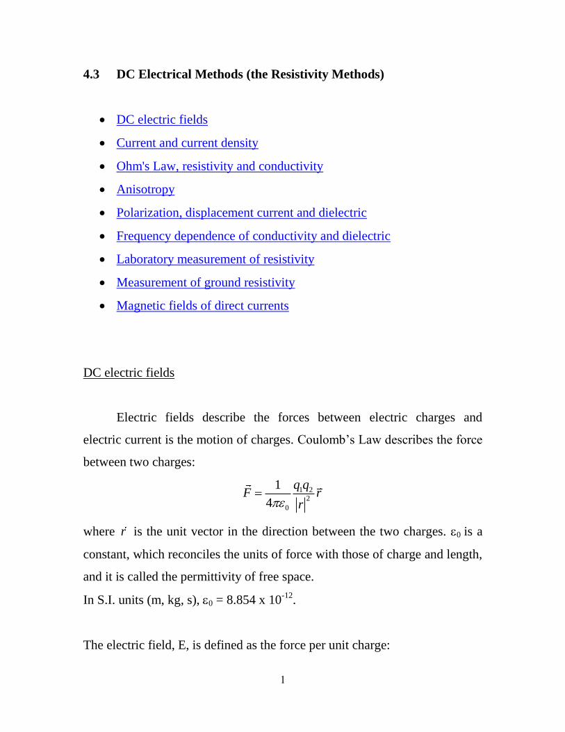
4.3 DC Electrical Methods (the Resistivity Methods)

DC electric fields

Current and current density

Ohm's Law, resistivity and conductivity

Anisotropy

Polarization, displacement current and dielectric

Frequency dependence of conductivity and dielectric

Laboratory measurement of resistivity

Measurement of ground resistivity

Magnetic fields of direct currents

DC electric fields

Electric fields describe the forces between electric charges and

electric current is the motion of charges. Coulomb’s Law describes the force

between two charges:

1 2

2

0

1

4

q qF r

r

where r is the unit vector in the direction between the two charges. 0 is a

constant, which reconciles the units of force with those of charge and length,

and it is called the permittivity of free space.

In S.I. units (m, kg, s), 0 = 8.854 x 10-12

.

The electric field, E, is defined as the force per unit charge:

2

2

2

1 0

1

4

F qE r

q r

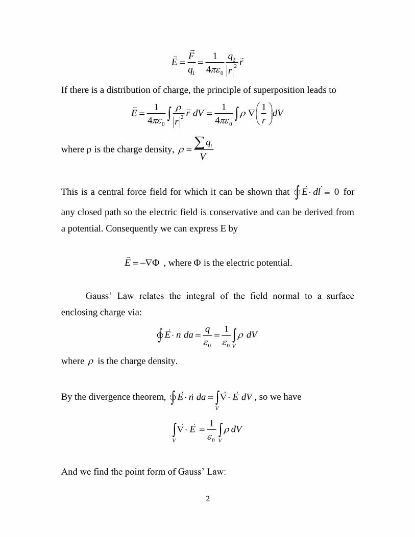
If there is a distribution of charge, the principle of superposition leads to

2

0 0

1 1 1

4 4E r dV dV

rr

where is the charge density, iq

V

This is a central force field for which it can be shown that 0E dl for

any closed path so the electric field is conservative and can be derived from

a potential. Consequently we can express E by

E , where is the electric potential.

Gauss’ Law relates the integral of the field normal to a surface

enclosing charge via:

0 0

1

V

qE n da dV

where is the charge density.

By the divergence theorem, V

E n da E dV , so we have

0

1

V V

E dV

And we find the point form of Gauss’ Law:

3

0

E

Current and current density

If the charges qi are moving with velocity vi then the current density is

defined by:

i iq vJ

Vol

So J is the charge per unit area moving past a point and has the units of

amperes per square meter (A/m2). If all the charges move uniformly:

J v

On a microscopic scale charge is conserved, so in a volume V where

charge is moving, the time rate at which charge passes through the enclosing

surface must be balanced by the time rate of charge build-up within the

volume.

Thus:

S

dJ n da dv

dt

and with the divergence theorem we can find the point relationship called

the Equation of Continuity:

0d

Jdt

4

Ohm’s Law, resistivity and conductivity

It is an experimental observation that the velocity that charges acquire

in an electric field in a medium is proportional to the field, so J is

proportional to E :

J E Ohm's Law

and is the conductivity in Siemens per meter, S/m.

The reciprocal of the conductivity is the resistivity, /E J in Ohm-

meters, Ohm-m or Ω-m.

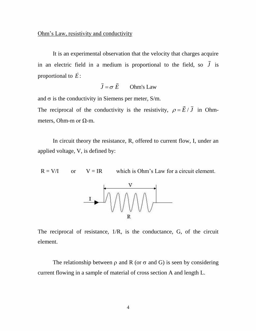
In circuit theory the resistance, R, offered to current flow, I, under an

applied voltage, V, is defined by:

R = V/I or V = IR which is Ohm’s Law for a circuit element.

The reciprocal of resistance, 1/R, is the conductance, G, of the circuit

element.

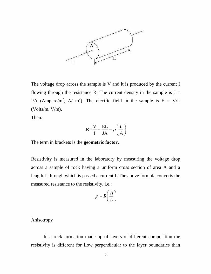
The relationship between and R (or and G) is seen by considering

current flowing in a sample of material of cross section A and length L.

5

The voltage drop across the sample is V and it is produced by the current I

flowing through the resistance R. The current density in the sample is J =

I/A (Ampere/m2, A/ m

2). The electric field in the sample is E = V/L

(Volts/m, V/m).

Then:

V ELR=

I JA

L

A

The term in brackets is the geometric factor.

Resistivity is measured in the laboratory by measuring the voltage drop

across a sample of rock having a uniform cross section of area A and a

length L through which is passed a current I. The above formula converts the

measured resistance to the resistivity, i.e.:

AR

L

Anisotropy

In a rock formation made up of layers of different composition the

resistivity is different for flow perpendicular to the layer boundaries than

6

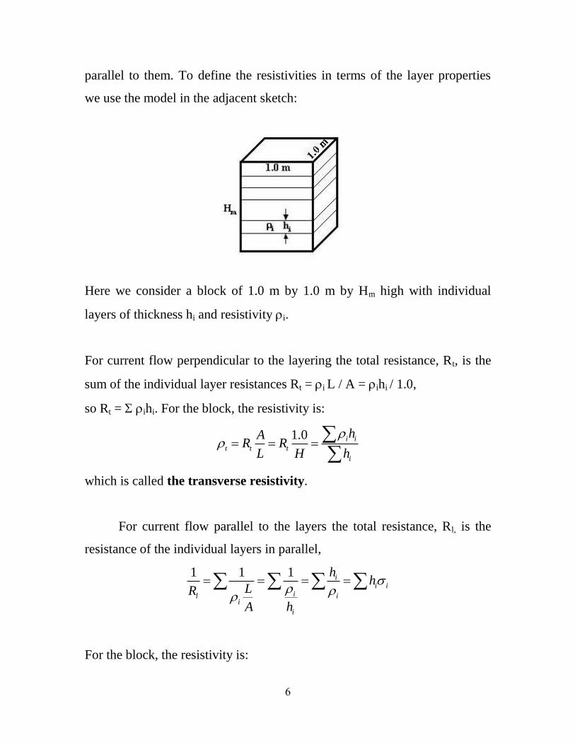
parallel to them. To define the resistivities in terms of the layer properties

we use the model in the adjacent sketch:

Here we consider a block of 1.0 m by 1.0 m by Hm high with individual

layers of thickness hi and resistivity i.

For current flow perpendicular to the layering the total resistance, Rt, is the

sum of the individual layer resistances Rt = i L / A = ihi / 1.0,

so Rt = ihi. For the block, the resistivity is:

1.0 i i

t t t

i

hAR R

L H h

which is called the transverse resistivity.

For current flow parallel to the layers the total resistance, Rl, is the

resistance of the individual layers in parallel,

1 1 1 ii i

il ii

i

hh

LR

A h

For the block, the resistivity is:

7

i

l l li

i

hAR R H

hL

which is called the longitudinal resistivity.

The ratio of the transverse to longitudinal resistivity is called the

coefficient of anisotropy, , which is given by:

i i i i

i i

h h

h

[Note that because of the square term in the denominator the square root of

is often used as the definition of the anisotropy.]

It is often the case that the layers form an alternating sequence of the same

two materials, for example sand and shale. If there are only two resistivities

present then the numerator factors into terms where the first sum is over the

layers with resistivity 1, and the second sum is over layers with resistivity

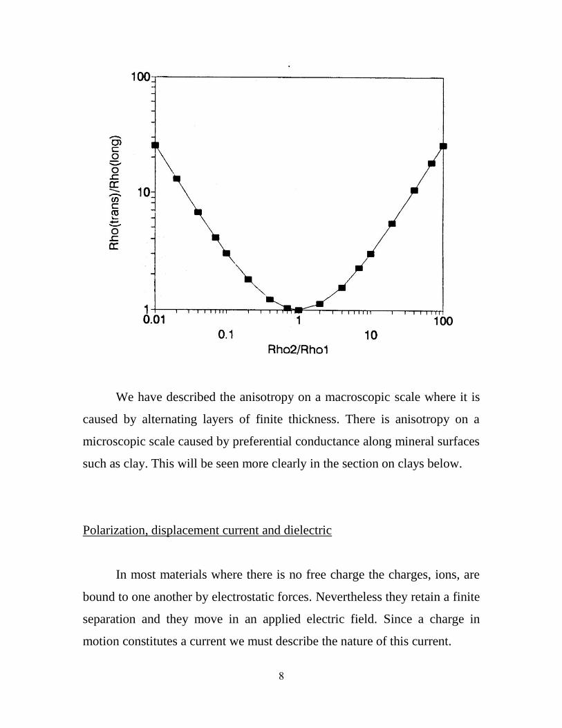
2. For example, if the two materials are in equal amounts:

2

1 2

1 2

0.25

The following plot shows this anisotropy as a function of the ratio of the two

resistivities.

8

We have described the anisotropy on a macroscopic scale where it is

caused by alternating layers of finite thickness. There is anisotropy on a

microscopic scale caused by preferential conductance along mineral surfaces

such as clay. This will be seen more clearly in the section on clays below.

Polarization, displacement current and dielectric

In most materials where there is no free charge the charges, ions, are

bound to one another by electrostatic forces. Nevertheless they retain a finite

separation and they move in an applied electric field. Since a charge in

motion constitutes a current we must describe the nature of this current.

9

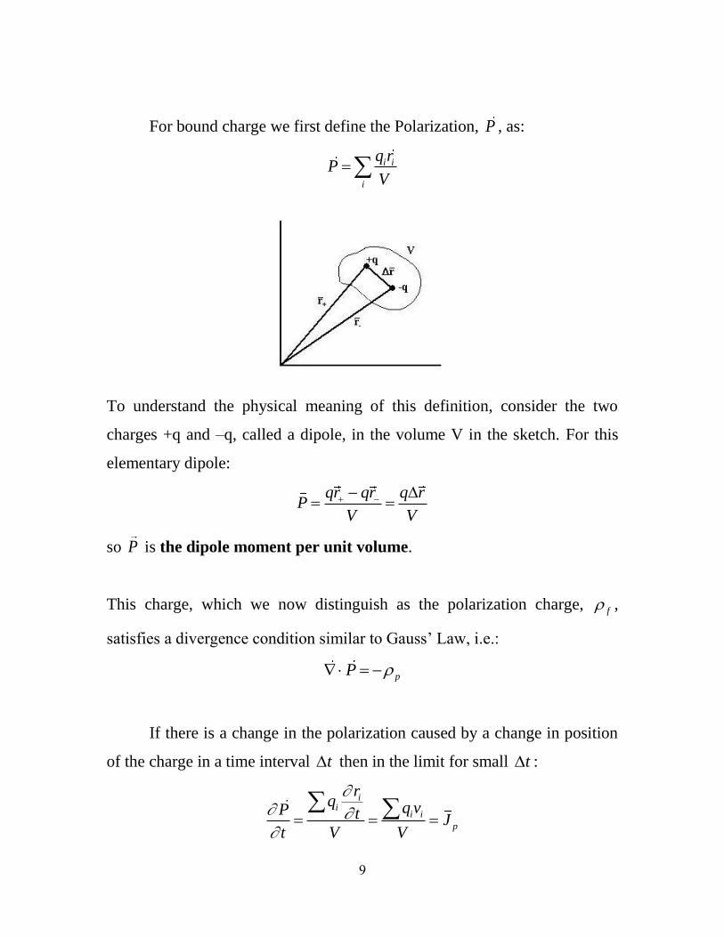
For bound charge we first define the Polarization, P , as:

i i

i

q rP

V

To understand the physical meaning of this definition, consider the two

charges +q and –q, called a dipole, in the volume V in the sketch. For this

elementary dipole:

qr qr q rP

V V

so P is the dipole moment per unit volume.

This charge, which we now distinguish as the polarization charge, f ,

satisfies a divergence condition similar to Gauss’ Law, i.e.:

pP

If there is a change in the polarization caused by a change in position

of the charge in a time interval t then in the limit for small t :

ii

i i

p

rq q vP t J

t V V

10

which is the polarization current.

This is real current and so it must satisfy the equation of continuity, i.e.:

0p

p

dJ

d t

We must also include both kinds of charge in Gauss’ law, so:

0

1f pE

and so:

0

1fE P

and therefore:

0 fE P

From this equation we define the displacement vector, D as:

0D E P

and fD

It has been found experimentally that P is a linear function of E at

low values of the field and so:

0 eP E

where e is the electric susceptibility.

Substituting this relationship in the definition of D we find,

0 01 eD E E E

where is the dielectric constant.

11

Frequency dependence of conductivity and dielectric

It is found experimentally that both conductivity and dielectric are

functions of frequency. The frequency dependence of conductivity, , is an

important property of rocks containing metallic minerals and clay and a field

method for measuring this property is called the induced polarization (IP)

method. Before discussing the mechanisms that cause this phenomenon we

can describe some of its properties from the basic behavior.

The frequency dependence is written:

J E

D E

In the time domain the current or displacement field is given by the

corresponding convolution operations:

J t s t E t

D t e t E t

where s and e are the Fourier transforms of the frequency dependent

conductivity and permittivity functions. , and J D E must be real in the time

domain and so s and e must also be real. Further both s(t) and e(t) must be

causal (no current or displacement field can occur before the causative

electric field) which implies that: 0 and 0s t e t Therefore in

writing the inverse transform back to frequency for either we have the form:

1

2

i ts t e dt

which, because , 0 s t , can be written as:

12

0 0

1cos sin

2 2

is t t dt s t t dt

.

We have found that both and must be complex if they are

functions of frequency (if they are not constant). The practical implication of

such a complex frequency dependence is that the current observed in rocks

or soils when they are subjected to a sinusoidal electric field is shifted in

phase with respect to the electric field and that the amount of phase shift

depends on the frequency. We will return to this topic later when we

describe the IP method in detail.

We have introduced the phenomenon of frequency dependent

resistivity in a general description of a method that was supposed to be

confined to DC or zero frequency. It should be understood that the electric

fields are conservative, that is they can be derived from the gradient of a

potential, if the additional electric fields created by time varying magnetic

fields are negligible. We shall see in the section on electromagnetic methods

that the induced electric fields depend on the induction number of the

problem, the product of the magnetic permeability conductivity and

frequency times some characteristic length squared of the problem, 2L .

As long as the frequency is low enough that the induction number is much

less than one then the DC description of the electric fields is valid.

13

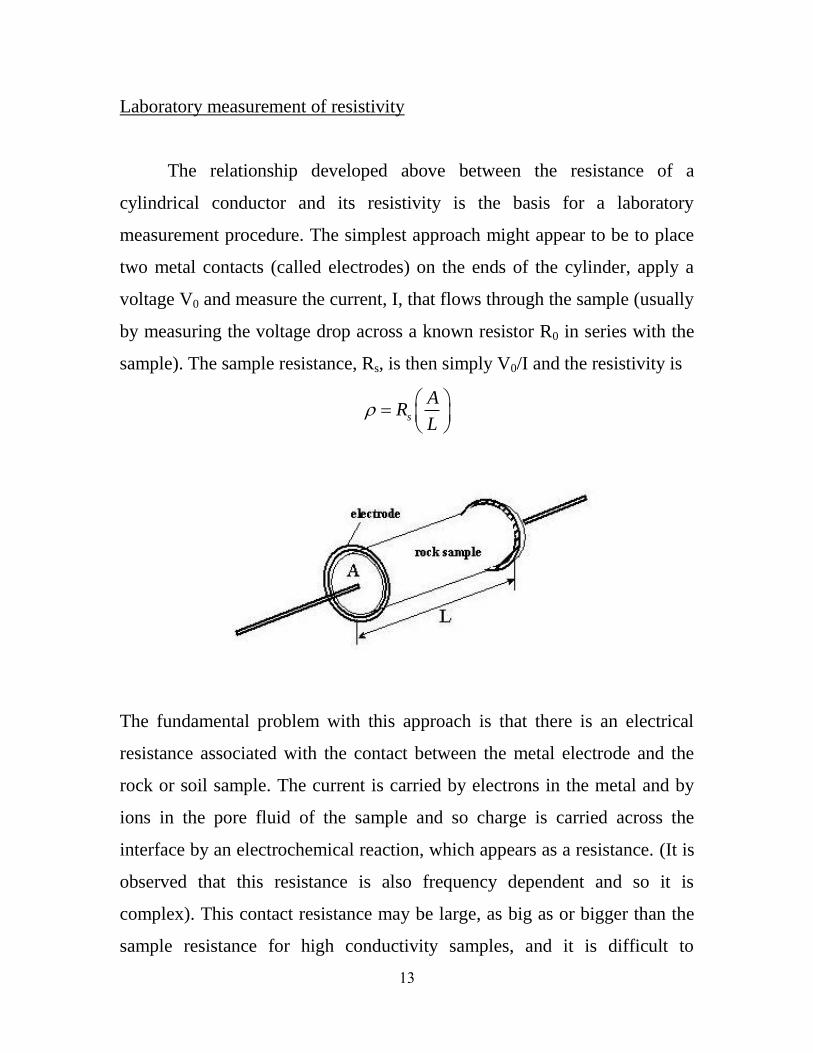
Laboratory measurement of resistivity

The relationship developed above between the resistance of a

cylindrical conductor and its resistivity is the basis for a laboratory

measurement procedure. The simplest approach might appear to be to place

two metal contacts (called electrodes) on the ends of the cylinder, apply a

voltage V0 and measure the current, I, that flows through the sample (usually

by measuring the voltage drop across a known resistor R0 in series with the

sample). The sample resistance, Rs, is then simply V0/I and the resistivity is

s

AR

L

The fundamental problem with this approach is that there is an electrical

resistance associated with the contact between the metal electrode and the

rock or soil sample. The current is carried by electrons in the metal and by

ions in the pore fluid of the sample and so charge is carried across the

interface by an electrochemical reaction, which appears as a resistance. (It is

observed that this resistance is also frequency dependent and so it is

complex). This contact resistance may be large, as big as or bigger than the

sample resistance for high conductivity samples, and it is difficult to

14

measure independently. For this reason the two-electrode method is not

suitable for most DC or low frequency measurements.

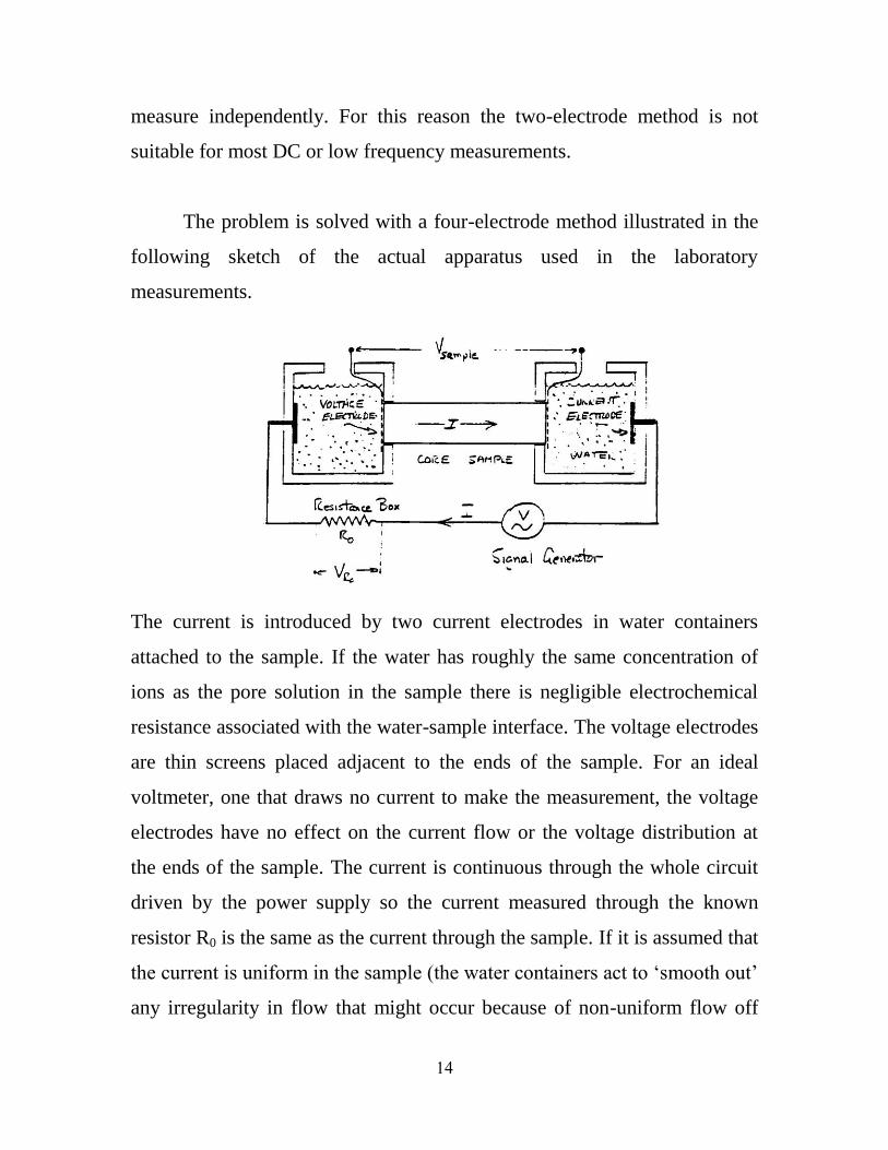
The problem is solved with a four-electrode method illustrated in the

following sketch of the actual apparatus used in the laboratory

measurements.

The current is introduced by two current electrodes in water containers

attached to the sample. If the water has roughly the same concentration of

ions as the pore solution in the sample there is negligible electrochemical

resistance associated with the water-sample interface. The voltage electrodes

are thin screens placed adjacent to the ends of the sample. For an ideal

voltmeter, one that draws no current to make the measurement, the voltage

electrodes have no effect on the current flow or the voltage distribution at

the ends of the sample. The current is continuous through the whole circuit

driven by the power supply so the current measured through the known

resistor R0 is the same as the current through the sample. If it is assumed that

the current is uniform in the sample (the water containers act to ‘smooth out’

any irregularity in flow that might occur because of non-uniform flow off

15

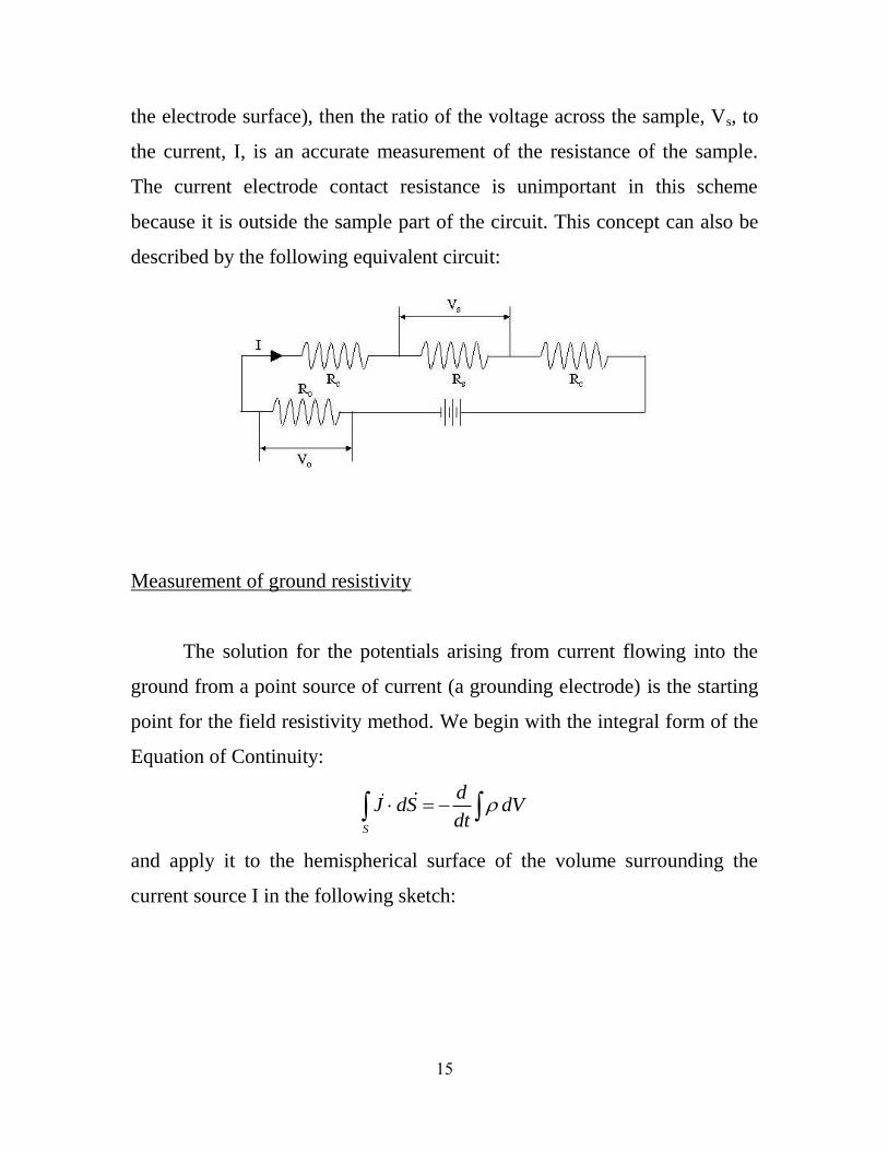
the electrode surface), then the ratio of the voltage across the sample, Vs, to

the current, I, is an accurate measurement of the resistance of the sample.

The current electrode contact resistance is unimportant in this scheme

because it is outside the sample part of the circuit. This concept can also be

described by the following equivalent circuit:

Measurement of ground resistivity

The solution for the potentials arising from current flowing into the

ground from a point source of current (a grounding electrode) is the starting

point for the field resistivity method. We begin with the integral form of the

Equation of Continuity:

S

dJ dS dV

dt

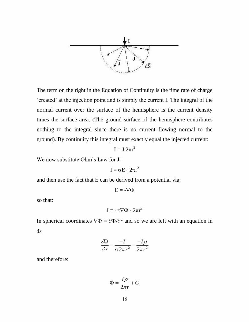
and apply it to the hemispherical surface of the volume surrounding the

current source I in the following sketch:

16

The term on the right in the Equation of Continuity is the time rate of charge

‘created’ at the injection point and is simply the current I. The integral of the

normal current over the surface of the hemisphere is the current density

times the surface area. (The ground surface of the hemisphere contributes

nothing to the integral since there is no current flowing normal to the

ground). By continuity this integral must exactly equal the injected current:

I = J 2r2

We now substitute Ohm’s Law for J:

I = E 2r2

and then use the fact that E can be derived from a potential via:

E = -

so that:

I = - 2r2

In spherical coordinates = /r and so we are left with an equation in

:

2 22 2

I I

r r r

and therefore:

2

IC

r

17

which is the potential of a point source of current on the surface of a uniform

half space.

Potential itself cannot be measured, only differences in potential.

Current cannot be created at a point - there must be another electrode

somewhere to return the current to the power supply (battery). In any real

system of electrodes there are always two for current and two for voltage

(potential difference). In practice, then, there is always an array of electrodes

used to measure the ground resistivity.

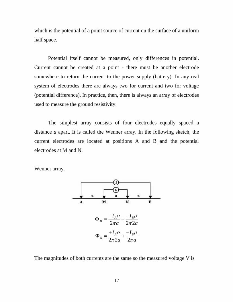
The simplest array consists of four electrodes equally spaced a

distance a apart. It is called the Wenner array. In the following sketch, the

current electrodes are located at positions A and B and the potential

electrodes at M and N.

Wenner array.

2 2 2

A BM

I I

a a

2 2 2

A BN

I I

a a

The magnitudes of both currents are the same so the measured voltage V is

18

V = M - N =1 1

1 12 2 2 2

I I

a a

So the resistivity of the ground is:

2V

aI

The term in brackets is the geometric factor for the array.

Over a uniform half space this array yields the true value of the

resistivity. Over an inhomogeneous half space the measured values of V and

I are put into the formula to yield the apparent resistivity, A. Over an

inhomogeneous half space A depends on a and on position on the surface.

A is really just a convenient way to express the measured voltage

normalized by the current and the dimensions of the array. The voltages

themselves depend on the current and on the separation. For example the

voltages in the Wenner array fall off as 1/a and the inhomogeneities produce

relatively small deviations from this dominant behavior. Plotting the

voltages on a log scale vs. a would be necessary but then the "anomalies"

would be hard to see. "Normalizing" by multiplying the voltages by a

corrects this plotting problem.

In practice one must be careful because the voltages do get very small

and become inaccurate for large spacings. Multiplying by a large (and

possibly inaccurate) spacing just yields a A with huge error.

There is one more important concept that can be demonstrated with

this simple array. It the current and potential electrodes are interchanged the

value of V/I, and hence A is unchanged. This is the Principle of

19

Reciprocity and it is true for any four electrode array over any arbitrary

inhomogeneous ground. It basically invalidates the usual explanation given

for the depth of investigation of DC resistivity methods which is based on

the penetration depth of the current. This argument suggests that as the

current electrodes are spaced farther apart the current penetrates more deeply

and hence ‘senses’ resistivities at greater depths. However the same

sensitivity can be achieved by placing the current electrodes close together

and measuring the voltage on widely spaced electrodes. Depth of exploration

has to be determined on a model by model basis for different arrays.

The basic concept of a resistivity sounding is that the volume of the

ground close to the array dictates the mean value of the apparent resistivity.

As the array expands larger and larger volumes of the ground are included

and so interpretation consists in determining the changes in actual ground

resistivity that cause the changes in apparent resistivity as the array grows.

This is a straightforward process for a horizontally layered ground, and the

response is almost intuitive for a two layer ground. For the first small

spacing of a sounding, when the array spacing is much smaller than the

thickness of the first layer, the apparent resistivity is the actual resistivity of

the first layer. As the array expands the apparent resistivity begins to

respond to the next layer (basement) and eventually at spacings greater than

the first layer thickness the apparent resistivity asymptotes to the basement

resistivity.

For geological situations where it cannot be assumed that the ground

is horizontally layered the resistivity survey must be carried out using a

combination of sounding and traversing – the whole array must be moved

20

laterally over the ground at the required number of spacings. Interpretation

then consists of matching the observed apparent resistivities to numerical

data for two or three dimensional models of the ground.

Magnetic fields of direct currents

The magnetic field associated with the current flow is not so easily

understood intuitively. There is, first of all, a field caused by the current in

the wire connecting the electrodes, which can be calculated by the law of

Biot and Savart. There is another component caused by the currents in the

ground. For a uniform or layered half space, integration of the magnetic field

from elements of current from the point source of current shows that the

horizontal field at the surface is simply half the value of the field of an

infinite line of current passing vertically through the electrode location

(Edwards and Nabhigian, 1991). If the ground is made up of uniform layers

the resulting magnetic fields measured on the surface are independent of the

ground conductivity and so depend only on the magnitude of the current and

the geometry of the source current line and the location of the magnetic field

detector. If the ground is inhomogeneous the ‘symmetry’ of the result is

broken and anomalous magnetic fields appear which depend on the

variations in the conductivity. Magnetometer surveys to detect these fields

are often called pure anomaly methods since they only respond to contrasts

in the subsurface. This magnetic variant of the DC resistivity method is

called the Magnetometric Resistivity (MMR) method.

21

The magnetic fields measured in the MMR method behave as DC

fields as long as actual frequency used in the measurements is such that the

induction number is small.