4286 IEEE TRANSACTIONS ON INFORMATION THEORY, VOL. …newport.eecs.uci.edu/~swindle/pubs/j93.pdf4286 IEEE TRANSACTIONS ON INFORMATION THEORY, VOL. 63, NO. 7, JULY 2017 The Gaussian

4286 IEEE TRANSACTIONS ON INFORMATION THEORY, VOL. 63, NO. 7, JULY 2017

The Gaussian CEO Problem for Scalar SourcesWith Arbitrary Memory

Jie Chen, Member, IEEE, Feng Jiang, Member, IEEE, and A. Lee Swindlehurst, Fellow, IEEE

Abstract— In this paper, we consider the achievablesum-rate/distortion tradeoff for the Gaussian central estimationofficer (CEO) problem with a scalar source having arbitrarymemory. We describe how the arbitrary memory problem canbe fully characterized by using known results for the vectorCEO problem, and then we formulate the variational problemof minimizing the sum-rate subject to a distortion constraint. Tosolve the problem, we extend the conventional Lagrange methodand show that if the solution exists, it should consist of a zeropart and a non-zero part, where the non-zero part is determinedby solving a set of Euler equations. By calculating the secondvariation of the min-sum-rate problem, a sufficient condition isalso found that can be used to determine if the necessary solutionresults in the minimal sum rate. The special case of two terminalsis examined in detail, and it is shown that an analytical solutionis possible in this case. Analysis and discussion with examples areprovided to illustrate the theoretical results. The general solutionobtained in this paper is shown to be compatible with the previousresults for cases such as the problem of rate evaluation for sourceswithout memory.

Index Terms— Multiterminal source coding, CEO problem,decentralized estimation, Gaussian sources with memory,variational calculus.

I. INTRODUCTION

W IRELESS sensor networks have been the subject ofactive research for the past decade, and they find many

uses in civil, industrial, commercial, and military applications.Such networks are often used for distributed sensing, in whichgeographically distributed sensors make measurements or localestimates and forward them to a fusion center, which conductsfurther processing to extract useful information from the data.

Manuscript received June 12, 2013; revised May 16, 2016; acceptedDecember 21, 2016. Date of publication May 10, 2017; date of currentversion June 14, 2017. This work was supported in part by the Air ForceOffice of Scientific Research under Grant FA9550-10-1-0310, and in part bythe National Science Foundation under Grant CCF-0916073. This paper waspresented at the 2012 46th Asilomar Conference on Signals, Systems andComputers. (Corresponding author: Jie Chen.)

J. Chen was with the Center for Pervasive Communications and Comput-ing and the Department of Electrical Engineering and Computer Science,University of California at Irvine, Irvine, CA 92697 USA. He isnow with Nokia Networks Arlington Heights, IL 60004 USA (e-mail:[email protected]).

F. Jiang was with the Center for Pervasive Communications and Computingand the Department of Electrical Engineering and Computer Science, Univer-sity of California at Irvine, Irvine, CA 92697 USA. He is now with IntelCorporation Santa Clara, CA 95054 USA (e-mail: [email protected]).

A. L. Swindlehurst is with the Center for Pervasive Communications andComputing and the Department of Electrical Engineering and ComputerScience, University of California at Irvine, Irvine, CA 92697 USA (e-mail:[email protected]).

Communicated by Y. Oohama, Associate Editor for Source Coding.Color versions of one or more of the figures in this paper are available

online at http://ieeexplore.ieee.org.Digital Object Identifier 10.1109/TIT.2017.2703136

In practice, the local measurements are typically quantizedprior to transmission, and there is clearly a trade-off betweenthe level of quantization (or equivalently the sensors’ transmis-sion rates) and the final estimation accuracy. With knowledgeof the required accuracy and the statistical characteristicsof the source and noise, the fusion center can optimallydetermine the sensors’ individual transmission rates and feedthis information back to the sensors in order to efficiently usethe available computing and communication resources.

This type of system is equivalent to indirect multiterminalsource coding, first studied in [1] and referred to as thecentral estimation officer (CEO) problem. In contrast to thedirect multiterminal source coding problem [2], where sensorsseparately measure different but correlated sources and thefusion center attempts to rebuild every source as accurately aspossible subject to a sum-rate constraint, each of the sensorsin the CEO problem receives a noisy observation of thesame source, which is later reconstructed at the fusion center.In order to characterize the rate region for the CEO problemwith a Gaussian source, Yamamoto and Itoh first studied theproblem in [3] for the two-terminal case, and later it was alsodiscussed independently by Flynn and Gray in [4]. The rateregion of the CEO problem was completely characterized fora memoryless Gaussian scalar source with an arbitrary numberof observers in [5]–[7]. As an extension to the scalar problem,the CEO model with a vector source was also consideredin [8]–[10].

In recent years, researchers have further attempted to extendthe CEO problem in various ways. Pandya et al. generalizedthe Gaussian CEO problem to the case of a Gaussian vectorsource where the observation is a noise-corrupted linear trans-formation of the source signal, and derived an upper bound onthe sum rate [11]. Compared to [11], Oohama’s model in [12]is more general, allowing the dimension of the source andobservation vectors to be different. In addition, [12] providesexplicit inner and outer bounds for the rate-distortion region,as well as a sufficient condition under which the lower andupper bounds are equal. This result was later improved on byYang and Xiong [13], who provided a new outer boundusing the entropy power inequality for a class of generalizedGaussian CEO problems, together with two sufficient condi-tions for equality between the outer and inner regions.

The end-to-end rate-distortion performance for differenttypes of source-to-destination communication networks hasalso been considered. Xiao and Luo [14] discussed the multi-terminal source and channel coding problem where quantizedobservations are sent through an orthogonal multiple accesschannel to a fusion center, and showed that separate source

0018-9448 © 2017 IEEE. Personal use is permitted, but republication/redistribution requires IEEE permission.See http://www.ieee.org/publications_standards/publications/rights/index.html for more information.

CHEN et al.: GAUSSIAN CEO PROBLEM FOR SCALAR SOURCES WITH ARBITRARY MEMORY 4287

and channel coding strictly outperforms the use of uncodedtransmissions. A variant of the traditional CEO problemwas studied in [15] where two terminals observe the samesource and deliver noisy measurements to a remote destinationthrough an intermediate relay node. A lower bound on thesum rate was found, and the achievable rates for two specialstrategies, compute-and-forward and compress-and-forward,were also derived. Kochman et al. [16] discussed a jointsource-channel coding scheme called rematch-and-forward forthe scenario where a Gaussian parallel relay network liesbetween the source and the remote fusion center.

Initiated by the proposal of designs based on generalizedcoset codes in [17] by Pradhan and Ramchandran, practicalcoding schemes for the CEO problem also have attractedattention in recent years. While the code design in [17] canbe used to arbitrarily allocate rates among source encodersin the achievable rate-distortion region, the gap between itsperformance and the theoretical limit is still somewhat large.Yang et al. [18] proposed a high-performance asymmetriccoding scheme for the CEO problem which is based on trellis-coded quantization followed by LDPC channel coding, andthey showed the resulting code rate is very close to thetheoretical bound for a Gaussian source. In [19], they extendedthe code design to attain the entire rate region through sourcesplitting and channel code partitioning.

Except for a brief discussion in [20], previous studiesall assume the sample sequence generated by the source ismemoryless. In this paper, we study the achievable sum-rateproblem for a Gaussian scalar source with arbitrary memory.First, we describe the system model for a source with memoryand we characterize the problem using known results forthe vector CEO problem. We then formulate the sum-ratecalculation as a variational calculus problem with a distortionconstraint, and show how to find a necessary condition whichthe solution to the problem must satisfy. Furthermore, weprovide a sufficient condition for determining if the necessarysolution achieves the minimal sum rate. A discussion of how tocompute the rate-distortion curve is then included, and we notethat the solution is compatible with previous findings in rate-distortion theory, which supports the validity of our results. Forthe special case of a system with two sensor nodes, we derivean analytic expression for the solution to the sum-rate problemand provide further examples to illustrate the theoretical resultsprovided by the necessary and sufficient conditions.

The rest of the paper is organized as follows. In Section II,we describe the system model and the necessary back-ground and preliminary theorems found in previous work.In Section III, we formulate the sum-rate optimization problemfor the L-terminal source coding case. In Section IV andSection V, we present our main results. Section IV providesthe necessary condition which can be used to find the solutionto the sum-rate problem, while Section V derives the sufficientcondition that can be used to check the optimality of thesolution obtained in Section IV. Analyses and discussionsof our theoretical results can also be found in Section V.Section VI focuses on the two-terminal case, for which wederive an analytic solution and present some representativeexamples. Section VII then summarizes the paper.

Fig. 1. Indirect multiterminal source coding (the CEO problem).

II. SYSTEM MODEL AND PRELIMINARIES

The indirect multiterminal source coding problem, or theso-called CEO problem, refers to separate lossy encoding andjoint decoding for multiple noise-corrupted observations of asingle data source. A block diagram model for the L-terminalCEO problem is illustrated in Fig. 1.

The fusion center is interested in recovering the real-valueddiscrete-time source sequence x(t), t = 0,±1, . . . , whereevery x(t) is a Gaussian random variable. Without loss ofgenerality, we can take the mean value of x(t) to be zerofor all t . The source sequence is assumed to be a stationarystochastic process with arbitrary memory; i.e., in contrast toan i.i.d. Gaussian source, the power spectral density (PSD)of x(t), denoted by �x (ω), is not necessarily constant overfrequency. We use vi (t) to indicate the measurement noise(or local estimation error) at sensor node i , and we assumeit is a real-valued zero-mean Gaussian process and i.i.d. intime. The observation at sensor i is given by yi (t) = x(t) +vi (t), and x(t) is the estimate of x(t) obtained at the fusioncenter. The error process is defined as x(t) = x(t) − x(t).Naturally, the more accuracy required in recovering the sourcesequence x(t), the higher the source coding rate has to be atthe L terminals. We are interested in studying the trade-offbetween the final fusion error and the sum source coding ratein the Berger-Tung achievable rate sense [7].

A. Berger-Tung Inner Bound and Sum Rate

In this section, we describe the calculation of the Berger-Tung achievable sum rate for a scalar Gaussian source witharbitrary memory. We use the method introduced in [21]to evaluate the Berger-Tung achievable sum rate, R(D),for a given target distortion D. Instead of directly calcu-lating the sum rate for an infinitely long Gaussian sourcesequence with arbitrary memory, we begin with the eval-uation of the achievable sum rate, Rn(D), for a Gaussiansource word x = (x(1), . . . , x(n)) and the correspondingreconstructed word x = (x(1), . . . , x(n)) with the distor-tion constraint E

{ 1n

∑nt=1(x(t)− x(t))2

} ≤ D. Letting thesize of the source word x go to infinity, we then have


R(D) = limn→∞ Rn(D). Similarly, the distortion constraintbecomes E{(x(t)− x(t))2} ≤ D due to the stationarity of thesource process.

For completeness, we briefly introduce the evaluation ofthe Berger-Tung sum rate for the problem of limited-sizevectors. Let yi , i = 1, . . . , L denote the noise-corruptedobservation vectors at the sensor nodes. From the discussionabove we know that all yi are also Gaussian distributed. Basedon [7]–[9], if there exist auxiliary random vectors wi , i =1, . . . , L such that wi → yi → (

x, y{i}c ,w{i}c)

forms aMarkov chain for all i , and if the distortion between x and xis no greater than D, the Berger-Tung achievable rate regionis the convex hull of

R(w1, . . . ,wL) ={(R1, . . . , RL)

∣∣∣

∑

i∈ARi ≥ I (yA; wA|wAc) ∀A ⊆ IL

},

(1)

where IL = {1, . . . , L}. Thus, the minimal sum rate is

Rn(D) = minw1,...,wL

1

nI (y1, . . . , yL ; w1, . . . ,wL). (2)

The Gaussianity of yi and wi results in [10]

Rn(D) = minw1,...,wL

1

2nlog

det(Cy) det(Cw)

det(Cyw), (3)

where Cy, Cw, and Cyw are the covariance matricesof vectors (yT

1 , . . . , yTL )

T , (wT1 , . . . ,wT

L )T and

(yT1 , . . . , yT

L ,wT1 , . . . ,wT

L )T , respectively. It is easy to

show that Cy, Cw, and Cyw are all block-symmetric matrices,and that each of their sub-blocks is Toeplitz. Throughout thepaper, all logarithms are assumed to take the natural base,and thus rates are always measured in nats.

B. Extension of the Toeplitz Distribution Theorem

In [21], evaluation of the rate-distortion function for thepoint-to-point problem relies on the Toeplitz distribution theo-rem [22]. Due to the block structure of the mutual informationmatrices in (3), we need to apply an extension [23] of theToeplitz distribution theorem to our problem, as discussednext.

Let T denote a c × c block matrix with n × n Toeplitzsubmatrix blocks, i.e.,

T =⎡

⎢⎣

T1,1 . . . T1,c...

. . ....

Tc,1 . . . Tc,c

⎤

⎥⎦

and

Ti, j =

⎡

⎢⎢⎢⎣

Ti, j (1) . . . . . . Ti, j (−n)Ti, j (2) Ti, j (1) . . . Ti, j (−n + 1)...

. . .. . .

...Ti, j (n) . . . Ti, j (2) Ti, j (1)

⎤

⎥⎥⎥⎦.

If T is also Hermitian, then from [23, Th. 3] we have

limn→∞

1

n

cn∑

k=1

F (λk(T)) = 1

2π

∫ π

−π

c∑

u=1

F(λu(�(ω)))dω, (4)

where F is an arbitrary function, λk for k = 1, . . . , cn andλu for u = 1, . . . , c are respectively the eigenvalues of T and�(ω), and

�(ω) =

⎡

⎢⎢⎢⎢⎢⎢⎢⎣

∞∑

k=−∞T1,1(k)e

− j kω . . .∞∑

k=−∞T1,c(k)e− j kω

.... . .

...∞∑

k=−∞Tc,1(k)e

− j kω . . .∞∑

k=−∞Tc,c(k)e− j kω

⎤

⎥⎥⎥⎥⎥⎥⎥⎦

.

In the next section, we will see how letting the size ofthe word x go to infinity can help us obtain a closed-formexpression for the mutual information and the distortion, andhence the problem formulation can be fully derived.

III. PROBLEM FORMULATION

In this section, we provide a full formulation of our problem.In order to calculate the mutual information, we appeal tothe extension of the Toeplitz distribution theorem describedabove. We also describe the optimal estimator structure andthe corresponding mean squared error (MSE), which is neededto define the distortion constraint. Finally we will see that therate evaluation is an infinite-dimensional variational problem.

A. Mutual Information

The calculation of mutual information is based on (3)and (4). We first assign the log function to F in (4), and thenlet the size of the matrices in (3) go to infinity so that theextension of the Toeplitz distribution theorem can be applied.After applying (4) to (3), we get the expression of the sumrate for the source-with-memory problem:

I (y1(t), . . . , yL(t);w1(t), . . . , wL(t))

= 1

4π

∫ π

−πlog

det �y(ω) det �w(ω)

det �yw(ω)dω, (5)

where

�y(ω)

=

⎡

⎢⎢⎢⎣

�y1(ω) �y1 y2(ω) · · · �y1 yL (ω)�y2 y1(ω) �y2(ω) · · · �y2 yL (ω)

......

. . ....

�yL y1(ω) �yL y2(ω) · · · �yL (ω)

⎤

⎥⎥⎥⎦

�w(ω)

=

⎡

⎢⎢⎢⎣

�w1(ω) �w1w2(ω) · · · �w1wL (ω)�w2w1(ω) �w2(ω) · · · �w2wL (ω)

......

. . ....

�wLw1(ω) �wLw2(ω) · · · �wL (ω)

⎤

⎥⎥⎥⎦

�yw(ω)

=

⎡

⎢⎢⎢⎢⎢⎢⎢⎢⎣

�y1(ω) · · · �y1 yL (ω) �y1w1(ω) · · · �y1wL (ω)...

. . ....

.... . .

...�yL y1(ω) · · · �yL (ω) �yLw1(ω) · · · �yLwL (ω)

�w1 y1(ω) · · · �w1 yL (ω) �w1(ω) · · · �w1wL (ω)...

. . ....

.... . .

...�wL y1(ω) · · · �wL yL (ω) �wLw1(ω) · · · �wL (ω)

⎤

⎥⎥⎥⎥⎥⎥⎥⎥⎦

,


Fig. 2. Forward test channels.

and �yi (ω), �yi y j (ω), �wi (ω), �wiw j (ω), �yiw j (ω),�wi y j (ω) are the auto- and cross-PSDs of the correspondingstochastic processes.

To further evaluate the mutual information expression of (5),we need to use the concept of forward test channels [24].Assuming the outputs of the dequantizers at the fusion center,wi (t), i = 1, . . . , L are also Gaussian, we can write the wholesystem in the forward test channel form [21]:

wi (t) = ai(t) ∗ yi (t)+ zi (t), i = 1, . . . , L, (6)

where ∗ represents convolution, ai (t), i = 1, . . . , L are vari-able real-valued functions to be determined, and zi (t), i =1, . . . , L represent quantization noise processes, which areassumed to be i.i.d. in time and independent from all yi (t). Theforward test channels are depicted in Fig. 2. Unlike problemswith memoryless sources, convolution is required here insteadof simple multiplication.

Given (6), the auto- and cross-PSD functions are given by:⎧⎪⎪⎪⎪⎪⎪⎪⎪⎪⎪⎪⎪⎪⎪⎪⎪⎪⎨

⎪⎪⎪⎪⎪⎪⎪⎪⎪⎪⎪⎪⎪⎪⎪⎪⎪⎩

�yi (ω) = �x (ω)+�vi (ω)

�wi (ω) = |Ai (ω)|2�yi (ω)+�zi (ω)

�wi yi (ω) = Ai (ω)�yi (ω)

�yiwi (ω) = A∗i (ω)�yi (ω)

�xyi (ω) = �x (ω)

�xwi (ω) = A∗i (ω)�x (ω)

�wi y j (ω) = Ai (ω)�x(ω) i = j

�yiw j (ω) = A∗j (ω)�x(ω) i = j

�yi y j (ω) = �x(ω) i = j

�wiw j (ω) = Ai (ω)A∗j (ω)�x (ω) i = j,

(7)

where i and j take values in IL , Ai (ω) is the discretetime Fourier transform of ai (t), and A∗

i (ω) is its conjugate.Plugging (7) into (5) and after a long series of mathemat-ical manipulations, we can simplify (5) to the followingexpression:

I (y1(t), . . . , yL(t);w1(t), . . . , wL(t))

= 1

4π

∫ π

−πlog

{∏Li=1

[�vi (ω)+�−1

mi(ω)

]

∏Li=1 �

−1mi (ω)

×(

1 +L∑

i=1

�x (ω)[�vi (ω)+�−1

mi(ω)

]−1)}

dω, (8)

where �mi (ω) = (|Ai (ω)|−2�zi (ω))−1

, and �zi (ω) is thePSD of zi (t). The sum rate is now parameterized in terms ofthe unknown functions �mi (ω), i = 1, . . . , L, from which allAi (ω) can be found.

B. MSE and Optimal Estimator

For memoryless sources, minimizing the MSE between x(t)and x(t) can be achieved by means of a simple estimator.Our problem involving sources with arbitrary memory is morecomplicated, since we need to estimate an entire stochasticprocess using multiple infinite-length sequences as the input.The estimator will have the form:

x(t) =L∑

i=1

hi (t) ∗ wi (t), (9)

where hi (t) for i = 1, . . . , L are optimal infinite-length filters.For known h1(t), . . . , hL(t), the MSE is given by

E{

x2(t)}

= E{(x(t)− x(t))2

}

= 1

2π

∫ π

−π

(

�x(ω)−L∑

i=1

�xwi (ω)H∗i (ω)

)

dω,

(10)

where Hi(ω) is the discrete-time Fourier transform of hi (t),and �xwi (ω) is the cross-PSD for x(t) and wi (t).

At first glance, it appears we may need to find an explicitexpression for Hi(ω), i = 1, . . . , L in order to connect theMSE solution with the sum-rate criterion in (8). The optimalestimator should satisfy the frequency domain Wiener-Hopfequations [25]:

H(ω)�w(ω) = �xw(ω), (11)

where H(ω) = [H1(ω), H2(ω), . . . , HL(ω)] and �xw(ω) =[�xw1(ω),�xw2(ω), . . . ,�xwL (ω)

]. Fortunately, we do not

need to solve (11). We simply need an expression for∑Li=1 �xwi (ω)H

∗i (ω), which can be found as follows:

L∑

i=1

�xwi (ω)H∗i (ω)

= �xw(ω)HH (ω)

(a)= �xw(ω)�−1w (ω)�H

xw(ω)

(b)= det[1 + �xw(ω)�

−1w (ω)�H

xw(ω)]

− 1

(c)= det[�w(ω)+ �H

xw(ω)�xw(ω)]

det �w(ω)− 1

=∑L

i=1[�2x(ω)]

[�vi (ω)+�−1

mi(ω)

]−1

1 +∑Li=1 �x (ω)

[�vi (ω)+�−1

mi (ω)]−1 , (12)

where (a) follows from (11), (b) uses the fact that thedeterminant of a scalar is the scalar itself, and (c) followsfrom the matrix determinant lemma [26].


Plugging (12) back into (10), we end up with thefinal MSE expression in terms of the unknown functions�mi (ω), i = 1, . . . , L:

E{

x2(t)}

= E{(x(t)− x(t))2

}

= 1

2π

∫ π

−π1

�−1x (ω)+∑L

i=1

[�vi (ω)+�−1

mi (ω)]−1 dω.

(13)

C. Full Formulation

With the above derivations, we can now give the fullformulation of the minimum sum-rate problem. Assuming thatthe rate is minimized when the distortion target is achievedwith equality, the rate evaluation problem is given by:

min�mi

1

4π

∫ π

−πlog

{∏Li=1

[�vi (ω)+�−1

mi(ω)

]

∏Li=1 �

−1mi (ω)

×(

1 +L∑

i=1

�x(ω)[�vi (ω)+�−1

mi(ω)

]−1)}

dω

(14)

s.t.1

2π

∫ π

−π1

�−1x (ω)+∑L

i=1

[�vi (ω)+�−1

mi (ω)]−1 dω

= D (15)

�mi (ω) ≥ 0, i = 1, . . . , L . (16)

This is a functional optimization problem and can be tackledvia the calculus of variations.

IV. NECESSARY CONDITION

In this section we derive a necessary condition that thesolution to the sum-rate problem (14)-(16) must satisfy. As wehave seen in Section III, the optimization in its final form isa constrained variational problem. In fact it can be regardedas an isoperimetric problem with additional inequality con-straints. The following theorem shows that in our formulationthe solution consists of a term that is zero together with anon-zero term that is determined by solving a set of Eulerequations. It is well known in the theory of the calculusof variations that solving the Euler equations results in anecessary condition.

Theorem 1 (Isoperimetric Problem With AdditionalInequality Constraints): Let ui and ψi , i = 1, . . . , n befunctions of ω. For the following functional optimizationproblem,

minu1,...,un

J (u1, . . . , un)

=∫ b

af (ω, u1, . . . , un, u′

1, . . . , u′n)dω (17)

s.t.∫ b

ag(ω, u1, . . . , un, u′

1, . . . , u′n)dω = D (18)

ui ≥ ψi , i = 1, . . . , n, (19)

the solution ui should consist of two parts: ψi and a functionno less than ψi . The latter can be obtained through solvingthe Euler equations with Lagrange multiplier λ:

fui − d

dωfu′

i+ λ

(gui − d

dωgu′

i

)= 0, i = 1 . . . , n. (20)

Proof: See Appendix A.We can apply Theorem 1 to the sum-rate problem (14)–(16),

where the corresponding functions and the upper and lowerbounds of integration are

ui (ω) = �mi (ω), i = 1, . . . , L,

f = 1

4πlog

{∏Li=1

[�vi (ω)+�−1

mi(ω)

]

∏Li=1 �

−1mi (ω)

×(

1 +L∑

i=1

�x(ω)[�vi (ω)+�−1

mi(ω)

]−1)}

,

g = 1/(2π)

�−1x (ω)+∑L

i=1

[�vi (ω)+�−1

mi (ω)]−1 ,

ψi (ω) = 0, i = 1, . . . , L,

a = −π,b = π.

We note that in our problem the functions f and g donot depend on the derivatives of u1, . . . , un , which means theEuler equations are not differential equations as often encoun-tered in variational problems. This fact eases the solving ofthe Euler equations, which are

(�vi (ω)�mi (ω)+ 1

)�vi (ω)

×⎛

⎝ 1

�x(ω)+

L∑

i=1

1

�vi (ω)+ 1�mi (ω)

⎞

⎠

2

+⎛

⎝ 1

�x(ω)+

L∑

i=1

1

�vi (ω)+ 1�mi (ω)

⎞

⎠ = λ, i = 1, . . . , L .

(21)

Problem (14)–(16) can also be formulated in another way,where the objective is to minimize the distortion (15) for atarget sum rate (14) equal to a given R. Based on the proof forTheorem 1, we find that the two formulations are essentiallythe same with the trivial difference that the Lagrange multiplierin the dual problem becomes 1/λ.

V. SUFFICIENT CONDITION

In this section we find a sufficient condition for prob-lem (14)–(16) to have a local minimum. To exploit thesufficient condition, we can first use Theorem 1 in Section IVto obtain a solution based on the necessary condition, and thenuse the sufficient condition discussed in this section to checkif the solution minimizes the sum rate.

As a first step, we prove the following lemma.


Lemma 2 (Degenerate Isoperimetric Problem): Let ui , i =1, . . . , n be functions of ω. For the following functional opti-mization problem to have a local minimum at (u1, . . . , un),

minu1,...,un

J (u1, . . . , un) =∫ b

af (ω, u1, . . . , un)dω (22)

s.t.∫ b

ag(ω, u1, . . . , un)dω = D, (23)

the sufficient condition is

Z(u1, . . . , un) � 0, (24)

where

Z(u1, . . . , un) =

⎡

⎢⎢⎢⎣

∂2ζ

∂u21

· · · ∂2ζ∂u1∂un

.... . .

...∂2ζ

∂un∂u1· · · ∂2ζ

∂u2n

⎤

⎥⎥⎥⎦,

ζ(ω, u1, . . . , un) = f (ω, u1, . . . , un)+ λg(ω, u1, . . . , un),

and λ is the associated Lagrange multiplier.Proof: See Appendix B.

Lemma 2 is referred to as a degenerate isoperimetricproblem because the derivatives of u1, . . . , un are explicitlyexcluded in (22) and (23), which is appropriate for ourminimum sum-rate problem. Using Lemma 2, we can furtherobtain the following theorem, which is directly applicable toproblem (14)–(16).

Theorem 3 (Degenerate isoperimetric problem with addi-tional inequality constraints): Let ui and ψi , i = 1, . . . , nbe functions of ω. For the following functional optimizationproblem,

minu1,...,un

J (u1, . . . , un) =∫ b

af (ω, u1, . . . , un)dω (25)

s.t.∫ b

ag(ω, u1, . . . , un)dω = D (26)

ui ≥ ψi , i = 1, . . . , n, (27)

the tuple (u1, . . . , un) is a local minimizer for J (u1, . . . , un)if there exist λ and ui , i = 1, . . . , n such that (28), as shownat the top of this page, is positive-definite, where zi in (28)should fulfill the following conditions:

1) for all i ,

zi ( fui + λgui ) = 0 (29)

holds;2) for a given i , if the Euler equation

fui + λgui = 0 (30)

holds, then zi = ±(ui − ψi )1/2. Otherwise zi = 0.

Proof: See Appendix C.

The problem in Theorem 3 is a degenerate isoperimetricproblem with additional inequality constraints, because itis merely the same problem described in Theorem 1 butenhanced with further requirements on ui .

A. Analysis and Discussion

1) Global Optimality: Theorem 3 only guarantees the exis-tence of a locally optimal solution. Since functional (14) isnot convex, a given local minimum is not guaranteed to be aglobal minimum. Thus we cannot safely claim that solving theequations in (21) will lead to the true Berger-Tung achievablesum rate, even if the sufficiency of the solution is verified byTheorem 3. However, since the number of potential solutionsis usually limited, theoretically it is possible to exhaustivelycalculate all rates associated with the corresponding solutions,and then choose the smallest of these as the global minimumachievable sum rate.

2) Evaluation of the Achievable Sum-Rate Function: Tocalculate the achievable sum rate as a function of the distortionD, one would normally substitute the solution to (21) into (15),and then solve it to get the value of λ. With knowledge of λ,the intermediate optimization variables,�m1(ω), . . . ,�mL (ω),can be determined and then used in (14) to completely deter-mine the achievable rate R. An alternative approach, similarto that explained in [21], is to first pick a value for λ, thenuse it in (21) to get �m1(ω), . . . ,�mL (ω), which are furthersubstituted into (14) and (15) to get the corresponding sumrate R and distortion D. The entire achievable rate-distortioncurve can be found in this fashion.

VI. SPECIAL CASE - TWO TERMINALS

In this section we first discuss the problem formulationand corresponding solution for a special case where thenumber of terminals is L = 2. Then some examples aregiven to illustrate the theoretical results obtained in previoussections. By numerically evaluating the sufficient condition inSection V, we also show that our solution is sufficient for afirst-order Gauss-Markov source process.

A. Formulation and Solution

In [27], a special case where there are only two terminalsin the system was considered. The optimal Wiener filters canbe explicitly obtained in this case:[

H1(ω)H2(ω)

]T

=[|A1|2|A2|2(�x�v1 +�x�v2 +�v1�v2)

+ |A1|2�y1�z2 + |A2|2�y2�z1 +�z1�z2

]−1

×[

A∗1�x(|A2|2�v2 +�z2)

A∗2�x (|A1|2�v1 +�z1)

]T

, (31)

Z(z1, . . . , zn) =⎡

⎢⎣

fu1 + 2z21 fu1u1 + λgu1 + 2λz2

1gu1u1 · · · 2z1zn fu1un + 2λz1zn gu1un...

. . ....

2znz1 fun u1 + 2λznz1gunu1 · · · fun + 2z2n funun + λgun + 2λz2

n gunun

⎤

⎥⎦ (28)


and the minimum sum-rate problem becomes

min�m1 ,�m2

1

4π

∫ π

−πlog

(�y1 +�−1m1)(�y2 +�−1

m2)−�2

x

�−1m1�

−1m2

dω

(32)

s.t.1

2π

∫ π

−π1

1�x

+ 1�v1+ 1

�m1

+ 1�v2+ 1

�m2

dω = D (33)

�m1 ≥ 0 (34)

�m2 ≥ 0. (35)

Note that Ai and all �’s are functions of ω, which has simplybeen dropped to save space.

While it is difficult to obtain a closed-form solutionto (14)–(16) for the general L-terminal case, an analyticalsolution is possible when L = 2. In this case, n = 2,ui = �mi and ψi = 0, and we can directly apply Theorem 1.Due to the fact that there are no derivatives of �i (ω) in theintegrand of the objective function, the Euler equations turnout to be merely algebraic rather than differential equations.After eliminating the infeasible solutions to these equations,we end up with the solution shown in (36)–(38), as shown atthe bottom of this page. Here the Lagrange multiplier λ shouldbe carefully picked so that (33) is fulfilled.

1) Compatibility With Known Results: The equivalencebetween our problem formulation and that in [7] can be shownvia a simple notation change to the functional optimizationproblem in (14)–(16). Our formulation is for sources withmemory, so the corresponding power spectral densities andintermediate functions are all functions of ω. For memorylesssources, these functions are constant in the ω-domain, and theformulation can be simplified as

min�mi

1

2log

{∏Li=1

[�vi +�−1

mi

]

∏Li=1 �

−1mi

×(

1 +L∑

i=1

�x

[�vi (ω)+�−1

mi

]−1)}

s.t.1

�−1x +∑L

i=1

[�vi +�−1

mi

]−1 = D

�mi ≥ 0, i = 1, . . . , L .

If we substitute the distortion constraint into the objectivefunction, we end up with

min�mi

1

2log

{�x

D

L∏

i=1

[�mi�vi + 1

]}

(39)

s.t.1

D= �−1

x +L∑

i=1

[�vi +�−1

mi

]−1(40)

�mi ≥ 0, i = 1, . . . , L . (41)

In the formulation of [7], the sum rate is given by

R(D)

= inf1D = 1

σ2X

+ 1σ2

N1+ 1μ2

1

+···+ 1σ2

NL+ 1μ2

L

1

2log+ σ 2

X

D

L∏

i=1

(μ2i σ

2Ni

+ 1),

(42)

where log+(x) is defined as max(0, log(x)). With the fol-lowing notational changes, �x ↔ σ 2

X , �mi ↔ μ2i , and

�vi ↔ σ 2Ni

, we can clearly see the equivalence between(39)–(41) and (42). With the constraints in (39)–(41), log+can be re-written as log.

It is also straightforward to show that in the memorylesssource case, our general solution reduces to that obtained, forexample, in [5], though the verification process is lengthy.We use L = 2 as an example. In this case we can directlycalculate the Lagrange multiplier:

λ = D�v1�v2 + D�v1�x + D�v2�x +�v1�v2�x

2D(D�v1�v2 + D�v1�x + D�v2�x −�v1�v2�x).

We can then substitute the expression for λ into (36) and (37)and further into the objective function of (39). We assume thatthe noise levels are equal at the observers, i.e., �v1 = �v2 =�v . After a long series of mathematical steps, the sum rate isobtained as

R = 1

2log

{�x

D

[�m1�v1 + 1

] [�m2�v2 + 1

]}

= 1

2log

{�x

D

(2D�x

D�v + 2D�x −�v�x

)2}

= − log

{1 − �v

2�x

(�x

D− 1

)}+ 1

2log

{�x

D

},

which is the same as the sum rate expression in [5] for L = 2.It is also possible to directly verify the equivalence with theL = 3 case, although it is somewhat more cumbersome todo so. The calculation for the general L-terminal case is verydifficult due to the complexity of the analytic form of thesolution; in particular, the expression for �mi becomes morecomplicated and thus more difficult to calculate as L grows,and thus so does the expression for the sum rate.

�m1 = max

(

0,− (�2v1(�x +�v2)

2 + 12�x�v1�v2(−λ�x�v2 +�x +�v2)− 1

2�2x�

2v2

− 12�x�v2�

)

�v1(�x�v1 +�x�v2 +�v1�v2)2

)

(36)

�m2 = max

(

0,− (�2v2(�x +�v1)

2 + 12�x�v1�v2(−λ�x�v1 +�x +�v1)− 1

2�2x�

2v1

− 12�x�v1�

)

�v2(�x�v1 +�x�v2 +�v1�v2)2

)

(37)

� = ±(λ2�2x�

2v1�2v2

+ 6λ�2x�

2v1�v2 + 6λ�2

x�v1�2v2

+ 6λ�x�2v1�2v2

+�2x�

2v1

+ 2�2x�v1�v2 +�2

x�2v2

+ 2�x�2v1�v2 + 2�x�v1�

2v2

+�2v1�2v2)

12 (38)


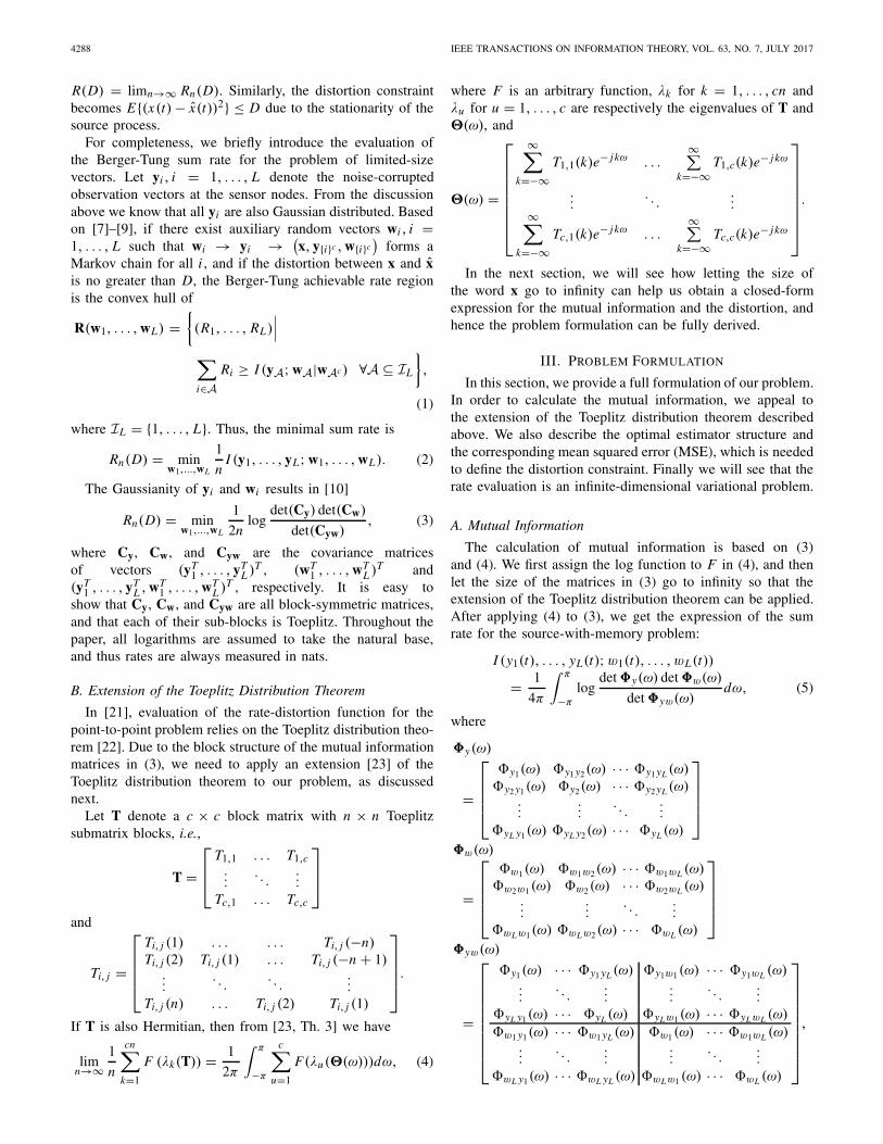
Fig. 3. Achievable sum rate versus target distortion (first-order Gauss-Markovprocesses).

B. Examples

The form of the solution for some special source processesis discussed below.

1) First-Order Gauss-Markov Process: A scalar discrete-time first-order Gauss-Markov process can be recursivelydefined as

x(t) = ρx(t − 1)+ u(t), (43)

where u(t) ∼ N (0, σ 2) is the driving noise. The autocorrela-tion function of this process is known to be

φx(t) = σ 2ρ|t |

1 − ρ2 , (44)

where |ρ| should be less than 1 or otherwise the process isnot stationary. The corresponding PSD is

�x (ω) = σ 2

1 − 2ρ cosω + ρ2 . (45)

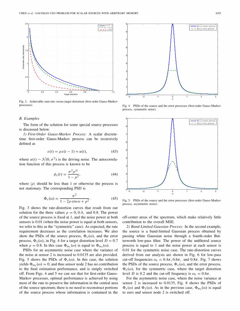
Fig. 3 shows the rate-distortion curves that result from oursolution for the three values ρ = 0, 0.4, and 0.8. The powerof the source process is fixed at 1, and the noise power at bothsensors is 0.01 (when the noise power is equal at both sensors,we refer to this as the “symmetric” case). As expected, the raterequirement decreases as the correlation increases. We alsoshow the PSDs of the source process, �x(ω), and the errorprocess, �x (ω), in Fig. 4 for a target distortion level D = 0.7when ρ = 0.8. In this case �m1(ω) is equal to �m2(ω).

PSDs for an asymmetric noise case where the variance ofthe noise at sensor 2 is increased to 0.0135 are also provided.Fig. 5 shows the PSDs of �x(ω). In this case, the solutionyields�m2(ω) = 0, and thus sensor node 2 has no contributionto the final estimation performance, and is simply switchedoff. From Figs. 4 and 5 we can see that for first-order Gauss-Markov processes, optimal performance is achieved by usingmost of the rate to preserve the information in the central areaof the source spectrum; there is no need to reconstruct portionsof the source process whose information is contained in the

Fig. 4. PSDs of the source and the error processes (first-order Gauss-Markovprocess, symmetric noise).

Fig. 5. PSDs of the source and the error processes (first-order Gauss-Markovprocess, asymmetric noise).

off-center areas of the spectrum, which make relatively littlecontribution to the overall MSE.

2) Band-Limited Gaussian Process: In the second example,the source is a band-limited Gaussian process obtained bypassing white Gaussian noise through a fourth-order But-terworth low-pass filter. The power of the unfiltered sourceprocess is equal to 1 and the noise power at each sensor is0.01 for the symmetric noise case. The rate-distortion curvesderived from our analysis are shown in Fig. 6 for low-passcut-off frequencies ωc = 0.4π, 0.6π, and 0.8π . Fig. 7 showsthe PSDs of the source process, �x (ω), and the error process,�x(ω), for the symmetric case, where the target distortionlevel D is 0.2 and the cut-off frequency is ωc = 0.6π .

For the asymmetric noise case, where the noise variance atsensor 2 is increased to 0.0135, Fig. 8 shows the PSDs of�x(ω) and �x (ω). As in the previous case, �m2(ω) is equalto zero and sensor node 2 is switched off.


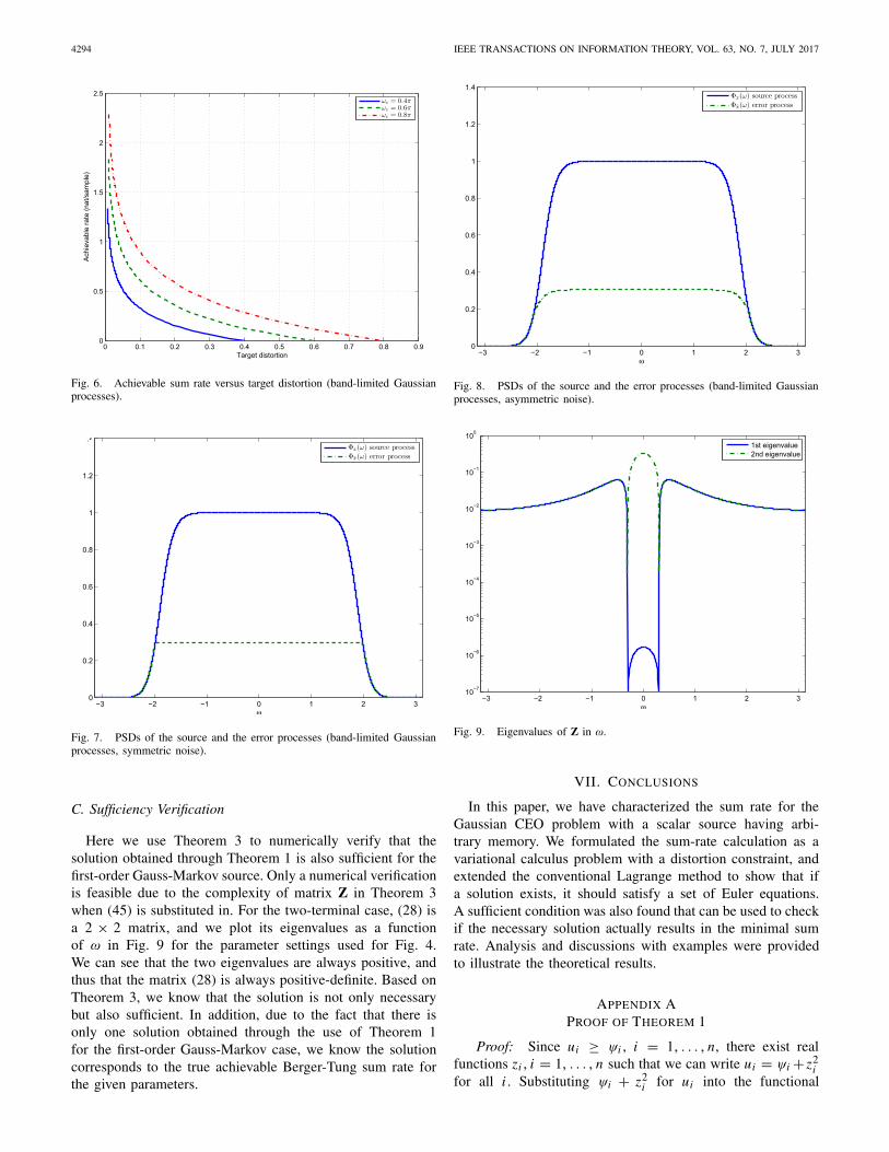
Fig. 6. Achievable sum rate versus target distortion (band-limited Gaussianprocesses).

Fig. 7. PSDs of the source and the error processes (band-limited Gaussianprocesses, symmetric noise).

C. Sufficiency Verification

Here we use Theorem 3 to numerically verify that thesolution obtained through Theorem 1 is also sufficient for thefirst-order Gauss-Markov source. Only a numerical verificationis feasible due to the complexity of matrix Z in Theorem 3when (45) is substituted in. For the two-terminal case, (28) isa 2 × 2 matrix, and we plot its eigenvalues as a functionof ω in Fig. 9 for the parameter settings used for Fig. 4.We can see that the two eigenvalues are always positive, andthus that the matrix (28) is always positive-definite. Based onTheorem 3, we know that the solution is not only necessarybut also sufficient. In addition, due to the fact that there isonly one solution obtained through the use of Theorem 1for the first-order Gauss-Markov case, we know the solutioncorresponds to the true achievable Berger-Tung sum rate forthe given parameters.

Fig. 8. PSDs of the source and the error processes (band-limited Gaussianprocesses, asymmetric noise).

Fig. 9. Eigenvalues of Z in ω.

VII. CONCLUSIONS

In this paper, we have characterized the sum rate for theGaussian CEO problem with a scalar source having arbi-trary memory. We formulated the sum-rate calculation as avariational calculus problem with a distortion constraint, andextended the conventional Lagrange method to show that ifa solution exists, it should satisfy a set of Euler equations.A sufficient condition was also found that can be used to checkif the necessary solution actually results in the minimal sumrate. Analysis and discussions with examples were providedto illustrate the theoretical results.

APPENDIX APROOF OF THEOREM 1

Proof: Since ui ≥ ψi , i = 1, . . . , n, there exist realfunctions zi , i = 1, . . . , n such that we can write ui = ψi + z2

ifor all i . Substituting ψi + z2

i for ui into the functional


optimization problem in Theorem 1, we end up with

minz1,...,zn

∫ b

aF(ω, z1, . . . , zn, z′

1, . . . , z′n)dω (46)

s.t.∫ b

aG(ω, z1, . . . , zn, z′

1, . . . , z′n)dω = D, (47)

where

F(ω, z1, . . . , zn, z′1, . . . , z′

n)

= f (ω, u1, . . . , un, u′1, . . . , u′

n)|ui=ψi +z2i

(48)

and

G(ω, z1, . . . , zn, z′1, . . . , z′

n)

= g(ω, u1, . . . , un, u′1, . . . , u′

n)|ui=ψi +z2i. (49)

It is clear that solving this problem for zi is equivalent tofinding the optimal ui .

The recast problem is an isoperimetric problem, which canbe solved by using the method of Lagrange multipliers. Lettingλ denote the multiplier, we have the Lagrangian as

∫ b

aF(ω, z1, . . . , zn, z′

1, . . . , z′n)dω

+ λ∫ b

aG(ω, z1, . . . , zn, z′

1, . . . , z′n)dω. (50)

Calculating the derivative of the Lagrangian with respect to zi

for all i and setting them to zero yields

Fzi − d

dωFz′

i+ λ

(Gzi − d

dωGz′

i

)= 0. (51)

Since

Fzi = 2zi fui + 2z′i fu′

i(52)

and

Fz′i= 2zi fu′

i, (53)

equation (51) becomes

zi

(fui − d

dωfu′

i+ λ

(gui − d

dωgu′

i

))= 0, (54)

which means either fui − ddω fu′

i+ λ

(gui − d

dω gu′i

)= 0 or

zi = 0. If zi = 0, ui should be equal to ψi . Otherwise itshould be the solution to

fui − d

dωfu′

i+ λ

(gui − d

dωgu′

i

)= 0, i = 1, . . . , n, (55)

which are exactly the Euler equations. This concludes theproof.

APPENDIX BPROOF OF LEMMA 2

We shall prove Lemma 2 by calculating the second variationof (25). As indicated in [28], if the second variation is stronglypositive in a neighborhood of (u1, . . . , un), then (25) has alocal minimum at (u1, . . . , un).

Proof: All admissible ui , i = 1, . . . , n must satisfy theconstraint

∫ b

ag(ω, u1, . . . , un)dω = D.

Utilizing this fact, we can rewrite (25) as

J (u1, . . . , un)

=∫ b

af (ω, u1, . . . , un)dω

=∫ b

a[ f (ω, u1, . . . , un)+ λg(ω, u1, . . . , un)] dω − λD,

(56)

where λ is the associated Lagrange multiplier. Let

ζ(ω, u1, . . . , un)

= f (ω, u1, . . . , un)+ λg(ω, u1, . . . , un), (57)

so that (56) can be written as

J (u1, . . . , un) =∫ b

aζ(ω, u1, . . . , un)dω − λD. (58)

Suppose we give (u1, . . . , un) an admissible increment(h1, . . . , hn). The selection of (h1, . . . , hn) is arbitrary as longas at least one of the hi is not identically zero in ω. We wantto calculate the second variation of J (u1 + h1, . . . , un + hn),which can be done using Taylor’s formula. After a series ofmathematical simplifications, the second variation of J can bewritten as

δ2 J (u1, . . . , un) = 1

2

∫ b

ahT Z(u1, . . . , un)h dω, (59)

where

h =⎡

⎢⎣

h1...

hn

⎤

⎥⎦ (60)

and

Z(u1, . . . , un) =

⎡

⎢⎢⎢⎣

∂2ζ

∂u21

· · · ∂2ζ∂u1∂un

.... . .

...∂2ζ

∂un∂u1· · · ∂2ζ

∂u2n

⎤

⎥⎥⎥⎦. (61)

The integrand of the second variation is a quadratic form in(h1, . . . , hn). Since the selection of (h1, . . . , hn) is arbitrary,the requirement that δ2 J (u1, . . . , un) is strongly positive isequivalent to requiring that Z(u1, . . . , un) is positive-definite.So the sufficient condition is

Z(u1, . . . , un) � 0. (62)

Due to the fact that (25) does not contain the derivatives ofui , i = 1, . . . , n, in this sufficiency proof we do not requirehi , i = 1, . . . , n to be continuously differentiable. So thelocal minimum guaranteed by Lemma 2 is not only a weakminimum but also a strong minimum [28].


Z(z1, . . . , zn) =⎡

⎢⎣

2 fu1 + 4z21 fu1u1 + 2λgu1 + 4λz2

1gu1u1 · · · 4z1zn fu1un + 4λz1zn gu1un...

. . ....

4znz1 funu1 + 4λznz1gunu1 · · · 2 fun + 4z2n fun un + 2λgun + 4λz2

ngunun

⎤

⎥⎦ (73)

APPENDIX CPROOF OF THEOREM 3

Proof: First we appeal to the mathematical technique usedin the proof of Theorem 1 to recast the problem. Since ui ≥ψi , i = 1, . . . , n, there exist real functions zi , i = 1, . . . , nsuch that we can write ui = ψi + z2

i for all i . Substitutingψi + z2

i for ui into the functional optimization problem inTheorem 3, we end up with

minz1,...,zn

∫ b

aF(ω, z1, . . . , zn)dω (63)

s.t.∫ b

aG(ω, z1, . . . , zn)dω = D, (64)

where

F(ω, z1, . . . , zn)

= f (ω, u1, . . . , un)|ui =ψi +z2i, (65)

and

G(ω, z1, . . . , zn)

= g(ω, u1, . . . , un)|ui=ψi +z2i. (66)

Applying Lemma 2 to this recast problem, we know thesufficient condition is

Z(z1, . . . , zn) � 0, (67)

where

Z(z1, . . . , zn) =

⎡

⎢⎢⎢⎣

∂2ζ

∂z21

· · · ∂2ζ∂z1∂zn

.... . .

...∂2ζ∂zn∂z1

· · · ∂2ζ∂z2

n

⎤

⎥⎥⎥⎦

(68)

ζ(ω, z1, . . . , zn) = F(ω, z1, . . . , zn)+ λG(ω, z1, . . . , zn),

(69)

and λ is the associated Lagrange multiplier.It is easy to show that for i = 1, . . . , n the first-order

derivatives are

∂ζ

∂zi= 2zi fui + 2λzi gui , (70)

and the second-order derivatives are

∂2ζ

∂z2i

= 2 fui + 4z2i fui ui + 2λgui + 4λz2

i gui ui (71)

∂2ζ

∂zi∂z j= 4zi z j fui u j + 4λzi z j gui u j . (72)

Plugging (71) and (72) back into (68), we get (73), as shownat the top of this page. Based on Lemma 2, we know if (73)is positive-definite then (u1, . . . , un) is guaranteed to be a

local minimum. Since multiplication of a matrix by a non-negative constant does not change the sign of its eigenvalues,it is equivalent to require (28) to be positive-definite.

In addition, from Theorem 1 we know

zi(

fui + λgui

) = 0, (74)

which means either zi = 0 or fui + λgui = 0. In the lattercase, we can let zi be either (ui − ψi )

1/2 or −(ui − ψi )1/2

due to the fact ui = ψi + z2i .

This completes the proof.

REFERENCES

[1] T. Berger, Z. Zhang, and H. Viswanathan, “The CEO problem,” IEEETrans. Inf. Theory, vol. 42, no. 3, pp. 887–902, May 1996.

[2] T. Berger and R. W. Yeung, “Multiterminal source encoding withone distortion criterion,” IEEE Trans. Inf. Theory, vol. 35, no. 2,pp. 228–236, Mar. 1989.

[3] H. Yamamoto and K. Itoh, “Source coding theory for multiterminalcommunication systems with a remote source,” IECE Trans., vol. E63,no. 10, pp. 700–706, Oct. 1980.

[4] T. Flynn and R. Gray, “Encoding of correlated observations,” IEEETrans. Inf. Theory, vol. 33, no. 6, pp. 773–787, Nov. 1987.

[5] Y. Oohama, “Rate-distortion theory for Gaussian multiterminal sourcecoding systems with several side informations at the decoder,” IEEETrans. Inf. Theory, vol. 51, no. 7, pp. 2577–2593, Jul. 2005.

[6] V. Prabhakaran, D. Tse, and K. Ramachandran, “Rate region of thequadratic Gaussian CEO problem,” in Proc. Int. Symp. Inf. Theory (ISIT),Jul. 2004, p. 119.

[7] J. Chen, X. Zhang, T. Berger, and S. B. Wicker, “An upper bound onthe sum-rate distortion function and its corresponding rate allocationschemes for the CEO problem,” IEEE J. Sel. Areas Commun., vol. 22,no. 6, pp. 977–987, Aug. 2004.

[8] S. Tavildar and P. Viswanath, “On the sum-rate of the vector GaussianCEO problem,” in Proc. Conf. Signals Syst. Comput. Rec. 39th AsilomarConf., Nov. 2005, pp. 3–7.

[9] J.-J. Xiao and Z.-Q. Luo, “Optimal rate allocation for the vectorGaussian CEO problem,” in Proc. 1st IEEE Int. Workshop Comput. Adv.Multi-Sensor Adapt. Process., Dec. 2005, pp. 56–59.

[10] J. Chen and A. L. Swindlehurst, “On the achievable sum rate ofmultiterminal source coding for a correlated Gaussian vector source,”in Proc. IEEE Int. Conf. Acoust. Speech Signal Process. (ICASSP),Mar. 2012, pp. 2665–2668.

[11] A. Pandya, A. Kansal, G. J. Pottie, and M. B. Srivastava, “Fidelity andresource sensitive data gathering,” in Proc. 42nd Allerton Conf., pp.1841–1850, Jun. 2004.

[12] Y. Oohama, “Indirect and direct Gaussian distributed source codingproblems,” IEEE Trans. Inf. Theory, vol. 60, no. 12, pp. 7506–7539,Dec. 2014.

[13] Y. Yang and Z. Xiong, “On the generalized Gaussian CEO problem,”IEEE Trans. Inf. Theory, vol. 58, no. 6, pp. 3350–3372, Jun. 2012.

[14] J.-J. Xiao and Z.-Q. Luo, “Multiterminal source–channel communicationover an orthogonal multiple-access channel,” IEEE Trans. Inf. Theory,vol. 53, no. 9, pp. 3255–3264, Sep. 2007.

[15] R. Soundararajan and S. Vishwanath, “Multi-terminal source codingthrough a relay,” in Proc. IEEE Int. Symp. Inf. Theory (ISIT), Aug. 2011,pp. 1866–1870.

[16] Y. Kochman, A. Khina, U. Erez, and R. Zamir, “Rematch and forward:Joint source/channel coding for communications,” in Proc. IEEE 25thConv. Electr. Electron. Eng. Israel, Dec. 2008, pp. 779–783.

[17] S. S. Pradhan and K. Ramchandran, “Generalized coset codes fordistributed binning,” IEEE Trans. Inf. Theory, vol. 51, no. 10,pp. 3457–3474, Oct. 2005.


[18] Y. Yang, V. Stankovic, Z. Xiong, and W. Zhao, “Asymmetric codedesign for remote multiterminal source coding,” in Proc. Data Compress.Conf. (DCC), Mar. 2004, p. 572.

[19] Y. Yang, V. Stankovic, Z. Xiong, and W. Zhao, “On multitermi-nal source code design,” IEEE Trans. Inf. Theory, vol. 54, no. 5,pp. 2278–2302, May 2008.

[20] S. Tung, “Multiterminal rate-distortion theory,” Ph.D. dissertation,School Elect. Eng., Cornell Univ., Ithaca, NY, USA, 1978.

[21] T. Berger, Rate Distortion Theory: A Mathematical Basis for DataCompression. Englewood Cliffs, NJ, USA: Prentice-Hall, 1971.

[22] U. Grenander and G. Szego, Toeplitz Forms and Their Applications.London, U.K.: Chelsea Publishing Company, 1964.

[23] H. Gazzah, P. A. Regalia, and J. P. Delmas, “Asymptotic eigen-value distribution of block Toeplitz matrices and application to blindSIMO channel identification,” IEEE Trans. Inf. Theory, vol. 47, no. 3,pp. 1243–1251, Mar. 2001.

[24] T. Cover and J. Thomas, Elements of Information Theory (Wiley Seriesin Telecommunications and Signal Processing). New York, NY, USA:Interscience, 2006.

[25] T. Kailath, A. H. Sayed, and B. Hassibi, Linear Estimation.Englewood Cliffs, NJ, USA: Prentice-Hall, 2000.

[26] D. A. Harville, Matrix Algebra From a Statistician’s Perspective. NewYork, NY, USA: Springer-Verlag, 2008.

[27] J. Chen, F. Jiang, and A. L. Swindlehurst, “The Gaussian CEO problemfor a scalar source with memory: A necessary condition,” in Proc.46th Asilomar Conf. Signals, Syst. Comput. (ASILOMAR), Nov. 2012,pp. 1219–1223.

[28] I. M. Gelfand and S. V. Fomin, Calculus of Variations (Dover Bookson Mathematics). New York, NY, USA: Dover, 2000.

Jie Chen (S’08–M’16) received the B.S. and M.S. degrees in CommunicationEngineering from Shanghai Jiao Tong University, Shanghai, China, in 1999and 2002, respectively, and the Ph.D. degree in Electrical Engineering atthe University of California, Irvine, in 2015. From 2002 to 2008, he wasan engineer at Huawei Technologies Co., Ltd. in China, where he wasinvolved in the research and development of algorithms for WCDMA andLTE wireless communication systems. His research interests include wirelesscommunications, statistical signal processing, multi-terminal source codingtheory, and information theory. He received the Best Student Paper Awardof the 46th Asilomar Conference on Signals, Systems and Computers. He isnow a research specialist at Nokia Networks.

Feng Jiang (S’10–M’15) received the B.S. degree in Communication Engi-neering and M.S. degree in Communication and Information System fromBeijing University of Posts and Telecommunications, Beijing, China, in 2004and 2008 respectively, and the Ph.D. degree in Electrical Engineering fromUniversity of California at Irvine, Irvine, CA, in 2015. From Oct. 2012to Mar. 2015, he worked as a student intern at Broadcom Corporation inthe Broadband, WPAN, and WLAN groups respectively. From Jun. 2015to Mar. 2016, he was a Staff II System Design Engineer at BroadcomCorporation, Sunnyvale, CA and contributed to the baseband design of linearMIMO receiver in the 802.11ax chipset. He is currently working as ResearchScientist in the Next Generation and Standards Group of Intel Corporation atSanta Clara, CA and his work focuses on the standardization of 802.11axand 802.11az. His research interests include statistical signal processingand convex optimization and he is co-author of a paper which receivedthe Student Paper Award at Asilomar Conference on Signals, Systems andComputers 2012.

A. Lee Swindlehurst (S’83–M’84–SM’89–F’04) received the B.S., summacum laude, and M.S. degrees in electrical engineering from Brigham YoungUniversity, Provo, Utah, in 1985 and 1986, respectively, and the Ph.D. degreein electrical engineering from Stanford University in 1991. From 1986–1990,he was employed at ESL, Inc., of Sunnyvale, CA, where he was involved inthe design of algorithms and architectures for several radar and sonar signalprocessing systems. He was on the faculty of the Department of Electrical andComputer Engineering at Brigham Young University from 1990–2007, wherehe was a Full Professor and served as Department Chair from 2003–2006.During 1996–1997, he held a joint appointment as a visiting scholar at bothUppsala University, Uppsala, Sweden, and at the Royal Institute of Technol-ogy, Stockholm, Sweden. From 2006–2007, he was on leave working as VicePresident of Research for ArrayComm LLC in San Jose, California. He iscurrently the Associate Dean for Research and Graduate Studies in the HenrySamueli School of Engineering at the University of California Irvine (UCI), aProfessor of the Electrical Engineering and Computer Science Department atUCI, and a Hans Fischer Senior Fellow in the Institute for Advanced Studiesat the Technical University of Munich. His research interests include sensorarray signal processing for radar and wireless communications, detection andestimation theory, and system identification, and he has over 250 publicationsin these areas.

Dr. Swindlehurst is a past Secretary of the IEEE Signal ProcessingSociety, past Editor-in-Chief of the IEEE JOURNAL OF SELECTED TOPICS

IN SIGNAL PROCESSING, and past member of the Editorial Boards for theEURASIP Journal on Wireless Communications and Networking, IEEE SignalProcessing Magazine, and the IEEE Transactions on Signal Processing. Heis a recipient of several paper awards: the 2000 IEEE W. R. G. Baker PrizePaper Award, the 2006 and 2010 IEEE Signal Processing Society’s Best PaperAwards, the 2006 IEEE Communications Society Stephen O. Rice Prize inthe Field of Communication Theory, and is co-author of a paper that receivedthe IEEE Signal Processing Society Young Author Best Paper Award in 2001.

Documents

4286 IEEE TRANSACTIONS ON INFORMATION THEORY, VOL. …newport.eecs.uci.edu/~swindle/pubs/j93.pdf4286 IEEE TRANSACTIONS ON INFORMATION THEORY, VOL. 63, NO. 7, JULY 2017 The Gaussian