Embed Size (px)
Citation preview

4/2011 environmentprotection
engineering
published quarterly
Wrocław 2011

Founding Editor
TOMASZ WINNICKI
Editor-in-Chief
KATARZYNA MAJEWSKA-NOWAK
Vice-Editors
Jerzy ZWOŹDZIAK, Lucjan PAWŁOWSKI
Assistant Editor
IZABELA KOWALSKA
Editorial Office
Faculty of Environmental Engineering Wrocław University of Technology
Wybrzeże Wyspiańskiego 27, 50-370 Wrocław, Poland
Publisher
Wrocław University of Technology, Wybrzeże Wyspiańskiego 27, 50-370 Wrocław
Oficyna Wydawnicza Politechniki Wrocławskiej Wybrzeże Wyspiańskiego 27, 50-370 Wrocław
http://www.oficyna.pwr.wroc.pl, e-mail: [email protected]
© Copyright by Oficyna Wydawnicza Politechniki Wrocławskiej, Wrocław 2011
Drukarnia Oficyny Wydawniczej Politechniki Wrocławskiej. Order No. 1169/2011.

CONTENTS
W. M. BUDZIANOWSKI, CO2 reactive absorption from flue gases into aqueous ammonia solutions: the NH3 slippage effect ................................................................................................................ 5
J. ĆWIKŁA, K. KONIECZNY, Treatment of sludge water with reverse osmosis ...................................... 21 W. DĄBROWSKI, Rational operation of variable declining rate filters ................................................ 35 W. GOLIMOWSKI, A. GRACZYK-PAWLAK, Influence of esterification of waste fats process parame-
ters on agricultural biofuel production facilities........................................................................... 55 B. KUCHARCZYK, W. TYLUS, Effect of promotor type and reducer addition on the activity of
palladium catalysts in oxidation of methane in mine ventilation air ............................................ 63 A. BIELSKI, Modelling of mass transport in watercourses considering mass transfer between phas-
es in unsteady states. Part II. Mass transport during absorption and adsorption processes .......... 71 M. ALWAELI, An economic analysis of joined costs and beneficial effects of waste recycling ......... 91 A. KOTOWSKI, H. SZEWCZYK, W. CIEŻAK, Entrance loss coefficients in pipe hydraulic systems ...... 105 E. STASZEWSKA, M. PAWŁOWSKA, Characteristics of emissions from municipal waste landfills...... 119 J. KRÓLIKOWSKA, Damage evaluation of a town’s sewage system in southern Poland by the
preliminary hazard analysis method ............................................................................................. 131 N. G. TURAN, B. MESCI, Adsorption of copper(II) and zinc(II) ions by various agricultural by-
-products. Experimental studies and modelling ........................................................................... 143


Environment Protection Engineering Vol. 37 2011 No. 4
WOJCIECH M. BUDZIANOWSKI*
CO2 REACTIVE ABSORPTION FROM FLUE GASES INTO AQUEOUS AMMONIA SOLUTIONS: THE NH3 SLIPPAGE EFFECT
Future deployment of NH3-based CO2 capture technology into coal-fired power plants will shift unwanted emissions from those currently comprising SO2, NOX and particulate matter towards those comprising NH3. This is due to volatility of ammonia. Therefore, the current paper aims at under-standing of NH3 slippage to flue gases from the NH3-based CO2 capture process and at identifying the opportunities to limit this unwanted slippage. The paper presents experimental and 2D modelling-based analysis of CO2 reactive absorption from flue gases into aqueous ammonia solutions in a fal-ling film reactor. The results enable one to characterise hydrodynamics of the falling film reactor, to analyse the effect of pH, pressure and temperature on CO2 absorption and NH3 slippage and to ex-plain the role of migrative transport of ionic species in total mass transport. It was found that NH3 slippage to the gaseous phase can be limited by alleviated operating temperatures, optimised pH, in-creased pressure and large CO2 absorption fluxes which force negative enhancement of NH3 mass transfer [16]. The NH3 slippage under CO2 capture conditions and under air stripping conditions is il-lustrated by experimental and simulation data. Finally, main approaches used for the integration of CCS systems into power plants are expounded.
1. INTRODUCTION
Recent atmospheric observations confirm that the concentration of CO2 in the at-mosphere has increased by nearly 30% for the last 150 years, with an accelerating trend in last years. The global mean concentration of CO2 in 2005 was 379 ppm, lead-ing to a radiative forcing of 1.66 W·mol–2. For the 1995–2005 decade, the growth rate of CO2 in the atmosphere was 1.9 ppm·yr–1 and the CO2 radiative forcing increased by 20%: this is the largest increase observed for any decade in at least the last 200 years. From 1999 to 2005, global CO2 anthropogenic emissions from fossil fuel and cement production increased at the rate of roughly 3% by year [1]. _________________________
*Faculty of Chemistry, Division of Chemical and Biochemical Processes, Wrocław University of Tech-nology, WybrzeżeWyspiańskiego 27, Wrocław, Poland, e-mail: [email protected]
W.M. BUDZIANOWSKI 6
There are two major carbon reservoirs which comprise 99.90% of the total Earth’s carbon, i.e. carbon rocks (limestone, chalk, dolomite) and organic-rich rocks (coal, oil, natural gas) [2]. Both those reservoirs are intensively exploited, e.g. in cement and en-ergy production, respectively; leading to large anthropogenic emissions of CO2 into the atmosphere. At the same time, Earth’s plant-covered areas are severely limited due to the civilisation development and thus the remaining plants are unable to recycle all the emitted carbon back to organic-rich rocks or at least into the soil. Also, it must be noted that carbon rocks formation in deep oceans is a very slow process which requires ab-sorption of atmospheric CO2 into oceans. When Earth’s temperature rises, the CO2 solu-bility in water alleviates, which limits the role of oceanic CO2 sink and can even the release of some CO2 dissolved in oceans amplifying the initial global warming.
Therefore, it can be concluded that recent human activities such as uncontrolled exploitation of natural carbon reservoirs and reduction in atmospheric CO2 recycle potentials by plants and oceans can contribute to net anthropogenic CO2 emissions as it is clearly evidenced by recent atmospheric measurements [1]. CO2 is the final prod-uct of numerous human activities which in large quantities accumulates in the atmos-phere causing dangerous climate changes.
Consequently, urgent deployment of renewable and nuclear energy technologies is needed, while CO2-intensive power plants must be integrated with carbon capture and sequestration (CCS). Therefore, the current paper provides modelling analysis of CO2 separation from flue gases by using aqueous ammonia solutions in a falling film reac-tor. The study investigates complex phenomena of mass transfer, chemical reactions, electrochemistry and hydrodynamics in very simple but offering realistic operating conditions reactor geometry. Results of the simulation and experiments illustrate the problem of NH3 slippage to the gaseous phase and discuss opportunities to limit this unwanted slippage.
2. MODELLING OF CO2 ABSORPTION INTO AQUEOUS AMMONIA SOLUTIONS
Absorption of CO2 into aqueous ammonia solutions has attracted attention as a po-tential CCS method for power plants relatively recently [3].
2.1. REACTION KINETICS AND THERMODYNAMICS
The most important liquid phase elementary chemical reactions in the CO2–NH3– –H2O system are presented in Table 1.

CO2 reactive absorption from flue gases 7
T a b l e 1
Elementary chemical reactions in the CO2–NH3–H2O system
Equation Process No.
2 3 2CO + NH NH COO H− +←⎯→ + formation of ammonia carbamate (1)
2 3CO +OH HCO− −←⎯→ formation of bicarbonate by combination of CO2 with hydroxyl ions (2)
23 3HCO CO H− − +←⎯→ + formation of carbonate (3)
3 2 4NH H O NH OH+ −+ ←⎯→ + hydrolysis of ammonia (4)
2H O OH H− +←⎯→ + dissociation of water (5)
Equations for reaction rates are summarised in Table 2.
T a b l e 2
Rates of elementary reactions from Eqs. (1)–(5)
No. Kinetics Source
(1) 2 3
11(1) CO NH
610001.66 10 exp GR C CR T
−⎛ ⎞= ⋅ ⎜ ⎟⎝ ⎠
[4]
(2) -2
10(2) CO OH
554204.32 10 exp GR C CR T
−⎛ ⎞= ⋅ ⎜ ⎟⎝ ⎠
[5, 6]
(3)–(5) instantaneous reactions [7] CO2 absorbed in ammonia solutions forms ammonia carbamate being a dominant
species at low CO2 loadings and in presence of excess NH3. For higher CO2 concentra-tions and hence for lower free ammonia concentrations, the equilibria of ammonia carbamate are shifted to favour bicarbonate formation. This shift allows higher CO2 loadings to be achieved in NH3-based systems compared with MEA-based systems where CO2 remains predominantly as a carbamate. Such observations have been con-firmed by Mani et al. [8] based on 13C NMR spectroscopy. However, the equilibria shifting towards bicarbonate requires higher pH in order to have higher concentrations of hydroxyl ions which promote bicarbonate formation (Eq. (2)). Carbamate formation is accompanied by H+ generation which lowers pH and favouring hydrolysis of free ammonia. When free ammonia is completely hydrolysed pH decreases and bicarbon-ate formation may stop due to relevant equilibria shifting.
Modelling of reversibility of reactions (1)–(5) is based on reaction equilibrium constants [7]. The rate of physical dissolution of gaseous CO2, NH3, and H2O in aque-ous solutions is relatively high. Therefore, equilibrium at the interface can be as-sumed. For CO2 and NH3 the Henry’s law may be introduced:
2 2 22 (g) 2 (l) CO CO COCO CO , P H C←⎯→ = (6)
W.M. BUDZIANOWSKI 8
3 3 33 (g) 3 (l) NH NH NHNH NH , P H C←⎯→ = (7)
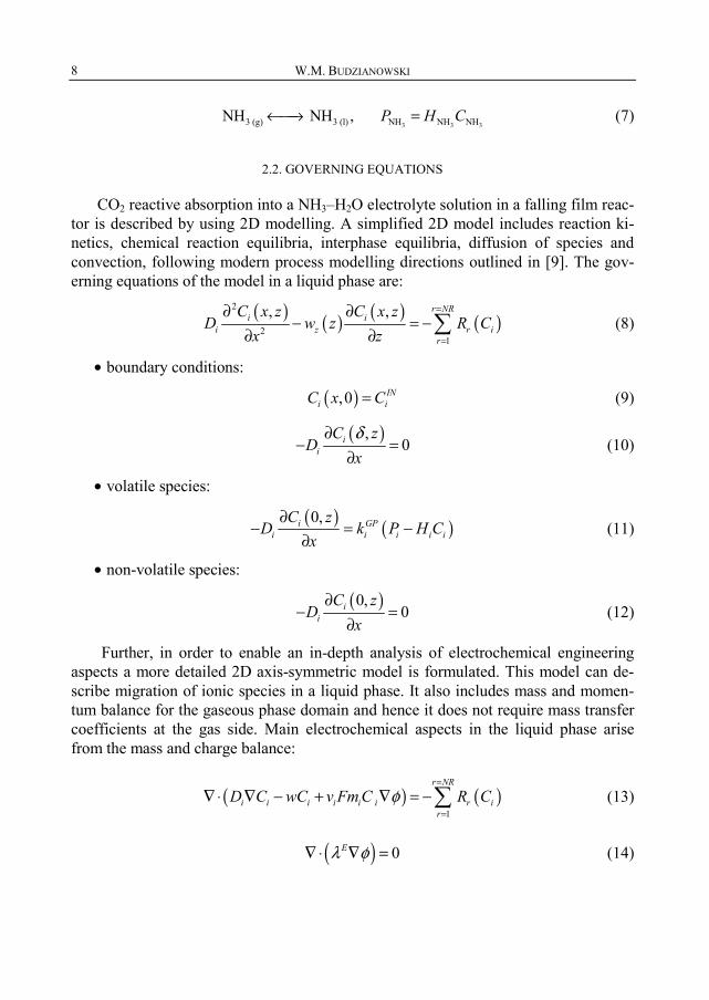
2.2. GOVERNING EQUATIONS
CO2 reactive absorption into a NH3–H2O electrolyte solution in a falling film reac-tor is described by using 2D modelling. A simplified 2D model includes reaction ki-netics, chemical reaction equilibria, interphase equilibria, diffusion of species and convection, following modern process modelling directions outlined in [9]. The gov-erning equations of the model in a liquid phase are:
( ) ( ) ( ) ( )
2
21
, , r NRi i
i z r ir
C x z C x zD w z R C
x z
=
=
∂ ∂− = −
∂ ∂ ∑ (8)
• boundary conditions:
( ),0 INi iC x C= (9)
( ),
0ii
C zD
xδ∂
− =∂
(10)
• volatile species:
( ) ( )0,i GPi i i i i
C zD k P H C
x∂
− = −∂
(11)
• non-volatile species:
( )0,
0ii
C zD
x∂
− =∂
(12)
Further, in order to enable an in-depth analysis of electrochemical engineering aspects a more detailed 2D axis-symmetric model is formulated. This model can de-scribe migration of ionic species in a liquid phase. It also includes mass and momen-tum balance for the gaseous phase domain and hence it does not require mass transfer coefficients at the gas side. Main electrochemical aspects in the liquid phase arise from the mass and charge balance:
( ) ( )1
r NR
i i i i i i r ir
D C wC v Fm C R Cφ=
=∇⋅ ∇ − + ∇ = −∑ (13)
( ) 0Eλ φ∇ ⋅ ∇ = (14)

CO2 reactive absorption from flue gases 9
2.3. A FALLING FILM REACTOR
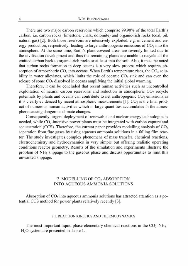
Falling-film reactors offer very simple geometries and well defined hydrodynam-ics which makes them to be well-suited for detailed kinetic studies. Besides, falling film reactors offer adjustable empty spaces and thus any crystallisation problems un-der highly concentrated and low temperature operating conditions can be limited. Fur-thermore, CO2 separation processes under industrially relevant short contact times conditions usually do not approach equilibrium conditions due to limited reaction and mass transport rates. Hence reaction and mass transfer kinetics-oriented studies are of primary importance for detailed design of such gas–liquid reactors [10]. Figure 1 illus-trates a falling film reactor utilised here for CO2 separation from flue gases by aqueous ammonia solutions. The falling film reactor is well suited for aforementioned kinetic studies and can be operated in practical hydrodynamic conditions.
Fig. 1. Scheme of the falling film reactor
3. ANALYSIS OF THE NH3 PROCESS
Among conventional CO2 reactive processes, a monoethanolamine (MEA) process has been comprehensively studied and successfully used in chemical plants for CO2 recovery. Although the MEA process is a promising method for the control of CO2 emissions from massive discharging plants [11], it is a relatively expensive option. In addition, it has several major disadvantages including slow absorption rate, low sol-vent capacity, amine degradation by SO2, NO2, HCl, HF and O2 from flue gases, high equipment corrosion rates, and high energy consumption during solvent regeneration (i.e. high heat of reaction compared with the CO2-NH3 system) [12].
In the MEA process SO2 and NOX must be removed prior to CO2 absorption. This preliminary costly removal might not be necessary when an aqueous ammonia solu-

W.M. BUDZIANOWSKI 10
tion is used which can capture all those acidic gases simultaneously with CO2. The products of absorption of CO2, SO2 and NOX into aqueous ammonia solutions are ammonium bicarbonate, ammonium sulphate and ammonium nitrate, respectively, which are well known fertilizers for certain crops. Unfortunately, ammonia salts have high solubility in water. Their removal by, e.g. crystallisation followed by filtration or sedimentation, can be enhanced under the chilled NH3 operating conditions (2–10 °C [13]) or by the addition of ethanol to aqueous ammonia solution which decreases solubility of salts [14]. Fertilisers from the NH3 process offer great unexplored poten-tial for cultivation of energy crops, i.e. biomass, which can tolerate fertilisers having lower quality and comprising some flue gas-derived impurities.
Further, an aqueous ammonia solvent is characterised in increased CO2 absorption capacity of 1.2 kg CO2/kg NH3, while for MEA it is only 0.4 kg CO2/kg MEA. There is little effect of oxidative degradation of ammonia as it comprises no carbon chains and thus it can offer improved solvent absorption/regeneration cycling. It has been shown [15] that CO2 absorption fluxes into ammonia can be 3 times higher than those into MEA under similar conditions. Also in [14] it has been shown that aqueous am-monia solvent has very high CO2 removal efficiency as compared with MEA or DGA solvents under similar operating conditions. Among major drawbacks of the NH3 process one can indicate ammonia volatility which leads to the contamination of flue gases. All available methods directed at NH3 removal [16] from diluted gases are costly. Therefore, to avoid ammonia slippage from the NH3 process careful attention must be paid to all process design and operation aspects.
It should be emphasised that future deployment of NH3-based CO2 capture into power plants can change the composition of unwanted emissions from the energy-generating sector. Namely, CO2 capture technologies using alkali aqueous solvents can offer simultaneous removal of SO2, NOX and particulate matter (PM) thus those emissions will be reduced. However, NH3-based CO2 capture technologies can lead to large increase of NH3 emissions [17] due to ammonia volatility. Therefore, the present study focuses on the opportunities for the reduction of NH3 emissions in NH3-based CO2 capture systems. In this context, effects of ammonia volatility, falling film reactor hydrodynamics, pH, migration in electrolyte solutions, elevated pressure and tempera-ture on the NH3 process are analysed and discussed.
3.1. EFFECT OF AMMONIA VOLATILITY
Field tests of CO2 capture into aqueous ammonia solutions indicate that a consid-erable ammonia slip to flue gases is frequently experienced under standard operating conditions. For instance Kozak et al. [18] have reported NH3 contents in flue gases up to 2000 ppmv due to desorber instabilities, and for more stable operation the NH3 slip has amounted up to 500 ppmv. Mathias et al. [19] have reported a smaller NH3 slip from their absorber, i.e. 242 ppmv in flue gases. Current permissible limits in several countries allow release of flue gases comprising less than 10 ppmv NH3. Therefore,

CO2 reactive absorption from flue gases 11
when utilising the NH3 process, one must guarantee limited ammonia vaporisation to the gaseous phase.
NH3 slippage to the gaseous phase can be reduced to meet the required level by controlling pH of the liquid, by making use of a negative enhancement of NH3 transfer effect and by thorough process and reactor designs. pH of the liquid can be conven-iently controlled by adjusting NH3 content in water. Further, NH3 transfer to the gase-ous phase can be negatively enhanced in situations when CO2 absorption flux is large enough to be able to substantially lower pH at the gas–liquid interface. Under the con-ditions of interfacial pH shift, NH3 slippage can be limited even under total driving forces promoting NH3 desorption [16].
Figure 2 shows NH3 slippage under air stripping [20] experimental conditions. It can be observed that the NH3 removal from the liquid is proportional to the stripping air flow rate. Such dependence is associated with gas–liquid phase equilibrium at-tained in the investigated conditions. Therefore, it can be concluded that the air-stripping process attains gas–liquid equilibrium at the investigated operating and geo-metrical ranges of parameters.
Fig. 2. NH3 slippage under air stripping experimental conditions, the effect of air flow rate on NH3 removal at 295 K,
2 3 2 3
3 3CO NH CO NH0, 0, 20 mol·m , 93 mol·m .IN IN IN INP C C− −= = = =
Experimental data for the packed-bed counter-current stripper with packing height of 1 m and packing diameter of
0.1 m, 15 mm ceramic Raschig rings
Under CO2 absorption conditions the phenomenon of NH3 slippage is more com-plex. Figure 3 illustrates that the liquid concentration of free (i.e. undissociated) NH3 decreases along the falling film reactor by means of two main mechanisms, i.e. by the reaction of NH3 with CO2 (Eq. (1)) and by NH3 desorption to the gas. As it is seen,

W.M. BUDZIANOWSKI 12
under operating conditions utilising large CO2 absorption flux, free NH3 is completely reacted or desorbed within around 15 cm of the falling film reactor length. For com-parison, when the desorption flux is switched off in the model and thus NH3 is con-sumed solely by the aforementioned reactive mechanism, the required length is con-siderably prolonged to around 30 cm. The contribution of the two competing NH3 consuming mechanisms strictly depends on process operating conditions [21]. It is expected that the contribution of NH3 slippage can be substantially reduced by using process design approaches.
Fig. 3. NH3 slippage under CO2 absorption conditions, the effect of NH3 desorption and reaction on NH3 content in the liquid phase along the absorber at 288 K.
2 3 2 3
4 3CO NH CO NH10 Pa, 0/1 Pa (without/with desorption), 0, 100 mol·m .IN IN IN INP P C C −= = = =
Simulations data from the simplified 2D model of the falling film reactor
The Henry’s constant of ammonia is much lower than that of CO2. HNH3 is typi-cally of the order of 1 Pa m3·mol–1 while HCO2 typically amounts to the order of 2000 Pa·m3·mol–1. For instance, at T = 288 K and CNH3 = 100 mol·m–3 (free ammonia), the gaseous phase equilibrium partial pressure is 100 Pa NH3, i.e. 1000 ppmv in flue gases (under atmospheric pressure) which means that free NH3 can easily desorb to the gas since its desorption driving force is relatively large and shown in Fig. 2 gas–liquid equilibrium is likely. Further, HNH3 is a rising function of temperature; therefore lower temperatures should disfavour ammonia volatility. However, the dependence of HNH3 on T is a relatively weak function, i.e. by decreasing temperature from 303 to 273 K, only a 5-fold drop in HNH3 is achieved. For instance, NH3 partial pressure equilibrated with 100 mol·m–3 of free NH3 solution under 273 K is still around 40 Pa NH3, i.e. 400 ppmv in flue gases (under atmospheric pressure). Consequently, new processes such as a chilled ammonia process [13] do not offer a complete solution to a NH3

CO2 reactive absorption from flue gases 13
volatility problem and thus some additional NH3 slippage limiting techniques are still necessary.
3.2. EFFECT OF PH ON MASS TRANSFER AND ON NH3 SLIPPAGE
In practice, in CO2 absorbers and solvent regenerators pH oscillates from 8,8 to 9,6 [12]. Ammonia slippage increases under high pH due to increased concentration of free NH3 in the liquid. On the other hand, under lower pH CO2 absorption is not en-hanced by chemical reactions and thus CO2 fluxes are degraded. Consequently, an optimum pH value should be found from economic evaluations of the whole CO2 capture system. An optimum NH3 content in water depends on CO2 loading, CO2 content in flue gases, temperature and pressure; however reasonable values can oscillate around 5%.
3.3. EFFECT OF HYDRODYNAMICS
In a falling film reactor, the liquid flow is solely driven by gravity while the gas flow is mainly driven by application of an external pressure, whereas gravity does virtually play no role. From present hydrodynamic analysis of the falling film reactor it can be deduced that liquid can be entrained by gas, especially for thin liquid films and large gas to liquid velocity ratios.
Fig. 4. Gas and liquid axial velocity profiles in a falling film reactor: dashed line – gaseous phase, solid line – liquid phase;
wL – liquid velocity, wG – gas velocity, wmax – maximum velocity in a relevant film. Simulation data from the detailed 2D axis-symmetric
model of the falling film reactor
Figure 4 illustrates results of simulation for a vertical falling film reactor (cf. Fig. 1). The gas flows in an upward direction and its velocity at the gas–liquid interface is substantially decreased compared with the bulk gas velocity. The liquid phase velocity profile is more complex. Under the operating conditions shown in Fig. 4 liquid en-
W.M. BUDZIANOWSKI 14
trainment is exhibited, at least close to the gas–liquid interface. At the gas–liquid in-terface velocity discontinuity is observed (note that the scales are different in Fig. 4). At the wall, liquid velocity approaches 0 due to the domination of friction forces. Con-sequently, maximum liquid velocity is attained somewhere in between the interface and the wall. This hydrodynamic effect is very disadvantageous for CO2 absorption fluxes since the velocity of saturated interfacial liquid is alleviated and hence its expo-sure time to the gas is prolonged. In contrast, this hydrodynamic effect can be benefi-cial for limiting NH3 slippage, especially under the conditions of simultaneous large CO2 absorption fluxes which can shift the equilibria at the gas–liquid interface to-wards complete consumption of free volatile ammonia.
It is expected that reactors with larger gas channels and of simpler geometry such as falling film reactors with thin liquid films can provide conditions for high CO2 re-moval, low NH3 slippage, ability to operation under high-pressure and to cope with salts crystallisation.
3.4. EFFECT OF MIGRATIVE SPECIES TRANSPORT
A NH3–CO2–H2O solution is a weak electrolyte and thus comprises numerous ionic species. Simulations conducted with the detailed 2D axis-symmetric model pro-vide some interesting insights into the NH3 process in this regard. Accordingly, apart from diffusive and convective motions involved, ionic species can also undergo mi-grative motion. According to the Nernst–Planck equation, migrative fluxes tend to reduce electrical potential gradients which arose here from diffusion of species (Eqs. (13), (14)). Such gradients of electrical potential can be formed when species substantially differ in diffusivities and when mass transfer fluxes are large. For in-stance, from the products of reaction in Eq. (1), H+ cations have 3-fold higher diffusiv-ity than carbamate anions. Hence, under a large CO2 absorption flux, faster diffusion of H+ from the gas–liquid interface creates small gradient of the electrical potential. In this electric field, carbamate anions formed diffuse and migrate in the same direction but H+ cations migrate and diffuse in the opposite one. This effect arises from the same direction of diffusion for all species produced in the liquid film due to CO2 ab-sorption and the opposite directions of migration of ions with negative and positive valences, i.e. anions and cations, within the electric field. Consequently, the transport of a carbamate anion (which carries CO2 and bounded NH3) is enhanced by its migra-tive motion and thus CO2 transport is favoured by a migrative mechanism from the interface to the liquid bulk. In a similar way, the migrative mechanism favours the transport of NH4
+ from the liquid bulk to the gas–liquid interface beneficially facilitat-ing ammonia transport. The above conclusions can also be deduced from Eq. (13) taking into account relevant valences of anions and cations as well as concentration and potential gradients formed in CO2 absorption into aqueous NH3. The migrative transport can only have indirect effect on NH3 slippage since NH3 is not an ionic species.

CO2 reactive absorption from flue gases 15
3.5. EFFECT OF ELEVATED PRESSURE
Elevated pressure affects vapour–liquid equilibria. It increases absorption fluxes and it alleviates desorption fluxes of both CO2 and NH3. Namely, under elevated pres-sure conditions partial pressures of CO2 and NH3 are increased by a factor comparable with a compression ratio applied. Increased partial pressures enhance CO2 absorption and beneficially degrade NH3 slippage. High pressures can be attained by e.g. the in-tegration of an absorber with a gas turbine. High pressures are necessary in a desorber unit (ca. 15 MPa) also with the aim to limit ammonia vaporisation from the hot regen-erated liquid. Thus the NH3 process is well suited for all pressurised combustion or IGCC power systems.
3.6. EFFECT OF TEMPERATURE
Experimental data on the effect of temperature on NH3 slippage under air stripping operating conditions is shown in Fig. 5. Increase in temperature facilitates NH3 slip-page due to decreased NH3 solubility in water, i.e. HNH3 increases with temperature.
Fig. 5. Effect of temperature on NH3 slippage under air stripping experimental conditions; T = 296 K,
2 3 2 3
3 3CO NH CO NH0, 0, 20 mol·m , 93 mol·m ,IN IN IN INP P C C− −= = = = aqueous ammonia
solution flow rate = 1.4×10⁻⁵ m3·s–1, stripping air flow rate = 6.7×10⁻³ m3·s–1. Experimental data from the packed-bed counter-current stripper with the packing height
of 1 m and packing diameter of 0.1 m utilising 15 mm ceramic Raschig rings
Again, the thermal behaviour of NH3 slippage under CO2 capture conditions is a bit more complex than under air striping conditions. Semi-batch CO2 absorption experiments [12] indicate that the net amount of CO2 absorbed decreases upon in-creasing temperature. This result arises from the decreased solubility of CO2 at higher temperatures since HCO2 increases upon increasing T. On the other hand, higher tem-

W.M. BUDZIANOWSKI 16
peratures tend to increase diffusivities of species and reaction rates. Besides, under CO2 capture conditions pH can strongly vary along the reactor due to CO2 absorption.
A thermal process control is a powerful tool in combating NH3 slippage [22–24]. However, a process utilising chilled NH3 [13] seems to be relatively expensive. Namely, the chilled NH3 process requires chilling of flue gases including the conden-sation of water, chilling of regenerated ammonia from a desorber and chilling of an absorber itself. The costs of chilling can be reduced in power plants having unlimited access to large cold water resources such as rivers or lakes.
3.7. EFFECT OF INTEGRATION INTO POWER PLANTS
Integration of CO2 capture systems into power plants necessitates advanced man-agement of energy and mass flows in order to reduce the CCS-induced power plant efficiency drop penalty. Besides, for the NH3 process the aspect of limited NH3 slip-page must be considered. Integration can benefit from the following measures:
• recirculation of flue gases back to combustion chambers which improves cycle efficiency and beneficially enriches CO2 in flue gases [25],
• thermal integration of processes [26–30], • utilisation of processes and apparatuses which enable one to reduce exergy losses
(large losses are typically linked with heaters, fans, compressors and reactors), • high-pressure CO2 separation, • optimising pressure and other parameters of steam supplied to a desorber, • optimising stripper operation and its configuration, • integration of CCS with more sophisticated energy technologies such as fuel
cells [31, 32] or bioenergies [33, 34]. More specifically, the NH3 process can benefit from highly reactive solvents such
as NH3, simultaneous removal of acidic gases (SO2 and NOX) and PM and direct inte-gration of a desorber with a heat recovery steam generator unit (HRSG). The NH3 process offers a reduction in regeneration energy requirements due to the higher load-ing capacity of an aqueous ammonia solution, the lower heat of reaction, and the lower heat of vaporisation when compared with standard MEA solutions.
4. CONCLUSIONS
Deployment of NH3-based CO2 capture into coal-fired power plants would shift unwanted emissions from those currently comprising SO2, NOX and particulate matter towards those comprising NH3 which necessitates research efforts directed at limiting NH3 slippage from NH3-based CO2 capture power systems. The presented experimen-tal and 2D simulation data of the NH3 process characterised the hydrodynamics of the
CO2 reactive absorption from flue gases 17
falling film reactor, determined the effect of pH, pressure and temperature on CO2 absorption and explained the role of migrative transport of ionic species in total mass transport. It was found that NH3 slippage could be limited by alleviated operating temperatures, optimised pH, increased pressure and large CO2 absorption fluxes, which forced negative enhancement of NH3 mass transfer to the gaseous phase. NH3 slippage under CO2 capture conditions and under air stripping conditions were illus-trated by simulation and experimental data. Approaches used in the integration of CCS systems into power plants were expounded.
SYMBOLS
CCS – carbon capture and sequestration E – activation energy, J·mol–1 HRSG – heat recovery steam generator K – chemical equilibrium constant, mol·m–3 or, m3·mol–1 or, mol2·m–6 kGP – mass transfer coefficient in the gaseous phase,, mol·m–2·s–1·Pa–1 M – molecular mass of species, kg·mol–1 MEA – monoethanolamine PM – particulate matter R – reaction rate, mol·m–3·s–1 C – molar concentration in liquid phase, mol·m–3 D – molecular diffusivity, m2·s–1 F – Faraday’s constant, A·s ·mol–1 H – Henry's constant, Pa m3·mol–1 m – mobility of ion, s·mol·kg–1 P – pressure or partial pressure, Pa r – radial coordinate, m RG – universal gas constant, J·mol–1·K–1 T – temperature, K v – valence of ion w – velocity, m·s–1 wZ – z component of velocity vector w, m·s–1 x – space coordinate, m δ – film thickness, m λ – thermal conductivity, J·mol–1·s–1·K–1 λE – electrical conductivity, S·mol–1 φ – electric potential in the electrolyte, V G – gaseous phase i, j – compound L – liquid phase r – reaction z – space or axial coordinate, m

W.M. BUDZIANOWSKI 18
GREEK SYMBOLS
δ film thickness, m λ thermal conductivity, J·mol–1·s–1·K–1 λE electrical conductivity, S·mol–1 φ electric potential in the electrolyte, V
SUBSCRIPTS AND SUPERSCRIPTS
G gaseous phase i, j compound L liquid phase r reaction
ACKNOWLEDGEMENTS
The author gratefully acknowledges the financial support from Wrocław University of Technology under grant No. S 10040/Z0311.
REFERENCES
[1] FORSTER P., RAMASWAMY V., ARTAXO P., BERNTSEN T., BETTS R., FAHEY D.W., HAYWOOD J., LEAN J., LOWE D.C., MYHRE G., NGANGA J., PRINN R., RAGA G., SCHULZ M., VAN DORLAND R., Changes in atmospheric constituents and in radiative forcing, [In:] Climate Change 2007: The Physical Science Basis. Contribution of Working Group I to the Fourth Assessment Report of the In-tergovernmental Panel on Climate Change, Cambridge University Press, Cambridge, 2007.
[2] FLORIDES G.A., CHRISTODOULIDES P., Global warming and carbon dioxide through sciences (Re-view), Environ. Int., 2009, 35, 390.
[3] OLAJIRE A.A., Energy, 2010, 35, 2610. [4] PUXTY G., ROWLAND R., ATTALLA M., Chem. Eng. Sci., 2010, 65, 915. [5] PACHECO M.A., ROCHELLE G.T., Ind. Eng. Chem. Res., 1998, 37, 4107. [6] PINSENT B.R.W., PEARSON L., ROUGHTON F.J.W., Transactions of the Faraday Society, 1956, 52,
1512. [7] BUDZIANOWSKI W.M., KOZIOŁ A., Chem. Proc. Eng., 1999, 20, 485. [8] MANI F, PERUZZINI M, STOPPIONI P., CO2 absorption by aqueous NH3 solutions: speciation of am-
monium carbamate, bicarbonate and carbonate by 13C NMR study, Green Chemistry, 2006, 8, 995 –1000.
[9] ZARZYCKI R., Diffusive methods in the description of environmental processes – historical overview, [In:] Modern Achievements in the Protection of Atmospheric Air, A. Musialik-Piotrowska, J.D. Rutkowski (Eds.), Polskie Zrzeszenie Inżynierów i Techników Sanitarnych, 2010, 407–410 (in Polish).
[10] BUDZIANOWSKI W.M., Rynek Energii, 2009, 83(4), 21. [11] GREER T., BEDELBAYEV A., IGREJA J. M., GOMES J. F., LIE B., Environ. Technol, 2010, 31 (1), 107. [12] YEH J.T., RESNIK K.P., RYGLE K., PENNLINE H.W., Fuel Process. Technol., 2005, 86, 1533. [13] GAL E., Ultra cleaning combustion gas including the removal of CO2, Patent No. WO2006022885,
2006.

CO2 reactive absorption from flue gases 19
[14] PELLEGRINI G., STRUBE R., MANFRIDA G., Energy, 2010, 35, 851. [15] LIU J., WANG S., ZHAO B., TONG H., CHEN C., Energy Proc., 2009, 1, 933. [16] BUDZIANOWSKI W.M., KOZIOL A., Chem. Eng. Res. Des., 2005, 83, 196. [17] KOORNNEEF J., RAMIREZ A., VAN HARMELEN T., VAN HORSSEN A., TURKENBURG W., FAAIJ A., At-
mos. Environ., 2010, 44, 1369. [18] KOZAK F., PETIG A., MORRIS E., RHUDY R., THIMSEN D., Energy Proc., 2009, 1, 1419. [19] MATHIAS P.M., REDDY S., O’CONNEL J.P., Energy Proc., 2009, 1, 1227. [20] HUANG H., XIAO X., YAN B., Desalin. Water Treatment, 2009, 8, 109. [21] SUN B.C., WANG X.M., CHEN J.M., CHU G.W., CHEN J.F., SHAO L., Ind. Eng. Chem. Res., 2009, 48,
11175. [22] KOTHANDARAMAN A., NORD L., BOLLAND O., HERZOG H.J., MCRAE G.J., Energy Proc., 2009, 1,
1373. [23] BUDZIANOWSKI W.M., KOZIOŁ A., Chem. Proc. Eng., 2001, 22, 301. [24] BUDZIANOWSKI W.M., KOZIOŁ A., Chem. Proc. Eng., 2000, 21, 741. [25] BUDZIANOWSKI W.M., Rynek Energii, 2010, 88(3), 151. [26] ROMEO L.M., ESPATOLERO, S., BOLEA I., Int. J. Greenh. Gas Con., 2008, 2, 563. [27] BUDZIANOWSKI W.M., MILLER R., Environ. Prot. Eng., 2008, 34(4), 17. [28] BUDZIANOWSKI W.M., MILLER R., Int. J. Chem. React. Eng., 2009, 7, A20. [29] BUDZIANOWSKI W.M., MILLER R., Can. J. Chem. Eng., 2008, 86, 778. [30] BUDZIANOWSKI W.M., MILLER R., Chem. Proc. Eng., 2009, 30, 149. [31] BUDZIANOWSKI W.M., Int. J. Hydrogen Energ., 2010, 35, 7454. [32] BUDZIANOWSKI W.M., Rynek Energii, 2009, 82 (3), 59. [33] GAJ K., KNOP F., TRZEPIERCZYŃSKA I., Environ. Prot. Eng., 2009, 35 (4), 73. [34] VALDEZ-VAZQUEZ I., POGGI-VARALDO H.M., Renew. Sust. Energ. Rev., 2009, 13(5), 1000.


Environment Protection Engineering Vol. 37 2011 No. 4
JOANNA ĆWIKŁA*, KRYSTYNA KONIECZNY**
TREATMENT OF SLUDGE WATER WITH REVERSE OSMOSIS
Considering the increasingly stringent requirements on the quality of treated wastewater intro-duced into surface or ground water, it is reasonable to reduce the loads of biogenic compounds pro-duced already at wastewater treatment plants in sludge treatment processes because sludge water produced in such treatment brings into the process cycle up to 20% more of nitrogen and phosphorus load. The paper presents the results of sludge water treatment in a reverse osmosis process. The con-centration of biogenic compounds in sludge water was successfully reduced by 95%. The tests were made using a pilot installation and laboratory installation. The concentrate produced in the reverse osmosis was treated by precipitating nitrogen and phosphorus compounds in form of struvite (NH4)Mg(PO4)×6H2O that can be next used as a fertiliser.
1. INTRODUCTION
Removal of biogenic compounds containing nitrogen and phosphorus from wastewater for many years has been at the focal point of both, researchers and end users. The issue has become especially vital after Poland’s accession into the Euro-pean Union and the adaptation of sewage treatment legislation with the EU standards. The Ordinance of the Minister of Environment valid from 2006 (and earlier from 2004) on the conditions to be fulfilled for discharging sewage to surface or ground water and on the substances especially harmful for the aquatic environment is setting forth that the permitted quantity of total nitrogen discharged to the environment with treated sewage for wastewater treatment plants with the ENI value of over 100 000 is only 10 mg N/dm3 or that the achieved reduction level should be at least 85%. The permitted value for wastewater treated at such plants was laid down at 1.0 mg/dm3 for phosphorus. The requirements were the consequence of adaptation Polish legislation with the EU solutions, in particular Directive 91/271/EEC of 21 May 1991 concerning urban wastewater treatment and Directive 98/15/EC of 27 February 1998 amending _________________________
*Przedsiębiorstwo Wodociągów i Kanalizacji Sp. z o.o., ul. Rybnicka 47, 44-100 Gliwice, Poland. **Silesian University of Technology, Faculty of Energy and Environmental Engineering,
ul. Akademicka 2A, 44-100 Gliwice, Poland, e-mail: [email protected]

J. ĆWIKŁA, K. KONIECZNY 22
Directive 91/271/EEC with respect to certain requirements established in Annex I thereof.
One should underline that the previous national requirements in this field provided that the permitted total nitrogen content in treated wastewater should not exceed 30 mg/dm3 and 5 mg/dm3 for phosphorus (Ordinance of the Minister of Environmental Protection, Natural Resources and Agriculture of 5.11.1991, Jol No. 116, item 503). Considering such low permitted concentration thresholds for N and P elements, it has become necessary to find efficient methods of removing biogenic compounds from sewage by methods other than conventional nitrification-denitrification systems.
Significant amounts of sludge are produced as a result of implementing new, ad-vanced sewage treatment technologies. Sludge undergoes, respectively, the stabilisa-tion and dewatering process at the treatment plant. The sludge water produced in such processes is in most cases recycled directly to the process cycle. Many researchers, therefore, have become interested in seeking alternatives to reduce nitrogen and phos-phorus loads generated already at the treatment plants as the removal of biogenic compounds from the internal process streams substantially decreases the nitrogen and phosphorus load flowing into the treatment plant’s main process [1].
Studies at wastewater treatment plants have revealed that the nitrogen and phos-phorus load returned with the sludge water produced in sludge treatment processes may account for up to 20–30% of the general load of biogenic compounds directed to biological reactors [2–4]. The C/N ratio is improved in the main process by removing nitrogen from the side streams, thus enhancing denitrification efficiency. It is an espe-cially attractive solution for the existing plants that are being upgraded for the purpose of carrying out or intensifying the biological removal of biogenic compounds.
There are significant issues involved in the treatment of water from digested sewage sludge dewatering such as: very high concentration of total nitrogen (occurring predomi-nantly in the form of ammonium nitrogen), high concentration of phosphorus compounds and suspended solid and marked variations in the concentration of contaminants.
High concentrations of nitrogen and phosphorus compounds is the effect of proc-esses occurring in mesophile sludge digestion – a hydrolysis of polyphosphates gath-ered in the cells of the bacteria responsible for the biological sewage dephosphatation process and the intensive proteins ammonification process.
2. CHARACTERISTICS OF SLUDGE WATER AND ITS TREATMENT METHODS
The following are the key parameters evaluated for sludge water [5] • COD 500–10 000 mg O2/dm3, • BOD5 150–1000 mg O2/dm3, • ammonium nitrogen 300–1000 mg N– +
4NH /dm3 (TKN typically 966 mg/dm3 [2]),

Treatment of sludge water with reverse osmosis 23
• phosphorus 30–100 mg P/dm3, • suspended solid = 400–13000 mg/dm3, • dissolved gases, including H2S, • heavy metals. Irrespective of the broad range of potential contaminant concentrations in sludge
water of various treatment plants, one should be aware that its composition in one particular plant may vary from day to day. The loads introduced with recirculated sludge water for particular plants may also differ, what is shown in a list provided as an example in Table 1 for several treatment plants in Poland [6].
T a b l e 1
Average estimated loads of contaminants introduced with recirculated sludge water at wastewater treatment plants [5]
Parameter Loads [%]
Białystok Ełk Łomża Suwałki OlsztynBOD5 3.5 26.0 0.47 erv 3.5 COD 6.5 31.0 4.8 2.4 1.0–4.5Total nitrogen 9.7 43.3 5.8 19.6 4.1–8.6Ammonium nitrogen 12.0 40.0 6.9 16.7 4.4–10Total phosporus 4.8 28.6 6.8 15.8 4.0–6.6Phosphates 5.7 27.8 7.2 15.3 3.9–7.8Suspended solid 6.0 42.7 0.06 6.7 0.6–4.1
In connection with the above, when analysing the operation of a specific plant it
becomes necessary to identify how much such composition may vary, or alternatively, which determinations may exhibit the highest fluctuations of results as such data is indispensable for deciding what treatment process for such water will be most appro-priate in a particular case.
In general, sludge water can be treated with methods falling into two groups: bio-logical processes and physiochemical processes. The following methods are most widespread for physiochemical processes:
• chemical precipitation, • hot air degassing, • stripping, • ion exchange. Each of the methods – both biological and physiochemical one, has its advantages
and disadvantages and many factors are decisive in choosing a specific one. Choosing the right method depends on the quality and variation of the treated water composi-tion, available funds as well as the conditions existing at the site. For instance, ammo-nia stripping with water steam will prove cost-effective if waste heat is available, whereas such costs will be substantial if such heat has to be produced particularly for

J. ĆWIKŁA, K. KONIECZNY 24
this method. If the high concentrations of ammonium nitrogen are also accompanied by the high concentrations of phosphorus compounds, the precipitation method (e.g. struvite crystallisation) may offer more benefits as compared to stripping because it allows one to remove both biogenic elements at the same time.
On the other hand, a certain disadvantage of new, unconventional biological methods is, most generally, that they focus more on removing nitrogen compounds, and their goal at the same time is not to remove phosphorus. The fact is also weighty that such methods are not conventional; therefore wastewater treatment plant re-searchers and environmental engineering designers are not familiar with them too well. The physiochemical methods, though, have been in use at the chemical industry for many years and are well known.
The paper focuses on the feasibility of reducing a load of biogenic compounds in sludge water using a combined method – reverse osmosis (RO) and then the precipita-tion of struvite from a concentrate in reverse osmosis. In practise, the RO process has been employed for treating run-offs from landfill sites (so-called leachates). Up till now the process has not, however, been used for sludge water at treatment plants. This is because the further handling of the concentrate has not been solved yet (in the case of leachate it is recycled to landfill sites where it gradually concentrates as water is evaporating naturally). Precipitation of ammonium and magnesium phosphate allows one not only to treat a concentrate from biogenic contaminants but also supplies a product usable as a fertiliser [7]. The advantage of concentrating contaminants be-fore their precipitation in such case is that the tanks and equipment used will require smaller volumes and throughputs. Moreover, the precipitation of the struvite sludge itself from the tanks should also be easier as compared to the precipitation method used directly for raw sludge water. It was also expected when choosing this method that the struvite crystals produced would be more regular than when precipitating this compound from unconcentrated solutions, and hence the struvite sludge will feature better sedimentation properties. A simple operation of a reverse osmosis installation and resistance to any installation startups and shutdowns was also of importance when choosing such a method. In addition, the installation is also easy to operate as the driv-ing force of the process is pressure gradient. Similarly, any change in the amount of the medium treated is not any problem – modular design of the device enables changes to its processing capacity by increasing or decreasing the area of the membrane ap-plied (by adding or removing the installation modules).
3. CHARACTERISTICS OF REVERSE OSMOSIS
Reverse osmosis, also referred to as hyperfiltration, serves for separating water (solvent) from the solute having small molecular mass. Single- and multivalent ions and low-molecular organic compounds are separated in this process. RO process is the opposite of natural osmosis phenomenon where the solvent is spontaneously passing

Treatment of sludge water with reverse osmosis 25
through a semipermeable membrane. If the membrane separates the solution from the solvent or separates two solutions with different concentration, then the solvent is flowing towards the solution having a higher concentration. External pressure equalis-ing the osmotic flow is called osmotic pressure characteristic of a specific solution. If a hydrostatic pressure builds up at the solution side exceeding the osmotic pressure, the solvent will permeate from the more concentrated solution to the more diluted one, therefore in the direction opposite than in the osmosis process. This process has been termed reverse osmosis [8].
The amount of water (solvent – Fw) passing through a semipermeable membrane characterised by Lp permeability (cm3/(cm2·s·Pa)) can be calculated from the following formula [8]:
Fw = Lp (P – π). The hydraulic performance of the process is directly proportional to the difference
between the external pressure P and the osmotic pressure π [9]. The amount of the solute (Fs) passing through the membrane depends on the con-
stant permeability of the solute B (cm/s) though, and the difference in concentrations ΔC for the solutions separated with the membrane:
sF B C= Δ .
The hydraulic performance of the process is measured with so-called membrane permeability (Lp) determined with the following formula:
rp
m
VLtS P
=Δ
,
where Vr – solution volume, t – time, Sm – membrane surface area, ΔP – pressure drop at both sides of the membrane [10].
Transmembrane pressure (TMP) used in reverse osmosis is higher than in an ul-trafiltration (UF) and microfiltration (MF) processes (3,5-10 MPa) [11], and the sol-vent (water) affinity to the membrane material plays a predominant role for choosing a membrane, whereas membrane pores are much less important as the separation mechanism is of the solving and diffusion nature [12,13].
4. EXPERIMENTAL
Sludge produced in the Central Wastewater Treatment Plant in Gliwice is intro-duced to mezophilic methane fermentation and next the dewatering process on Roedi-ger–Pasavant belt filter presses is performed. The sludge water produced during the

J. ĆWIKŁA, K. KONIECZNY 26
dewatering is recycled to the biological part of the plant and directed to the activated sludge chambers. The following parameters were evaluated for investigated sludge water: pH, COD, BOD5, ammonium nitrogen, nitrate nitrogen, total nitrogen, total phosphorus, phosphates, suspended solid, conductivity, calcium, magnesium. All analyses were made according to standards presented in Table 2. Studies were carried out between January 2005 and March 2009.
T a b l e 2
Variations in sludge water composition in January 2005–March 2009
Parameter Method of determination (Norm) Average Minimum Maximum
pH PN–C-04540/01:1990 7.58 7.3 8.0 COD, mg O2/dm3 PN–ISO 15705:2005 435.5 79.5 869.0
BOD5, mg O2/dm3 PB-5.4-01/23 publ. 02. 02.01.07 99.8 40 220
Ammonium nitrogen, mg N–NH4/dm3 PN–ISO 5664:2002 603.3 416 887
Nitrates nitrogen, mg N–NO3/dm3 PB-5.4-01/09 publ. 02. 02.01.07 5.48 0.5 24.3
Total nitrogen, mg N/dm3
PB-5.4-01/04 publ. 04. 02.02.09 PB-5.4-01/09 publ. 02. 02.01.07 PN–EN 25663:2001 PN–C-04576/14:1973
652.9 438.0 896.7
Total phosphorus, mg P/dm3 PB-5.4-01/08 publ. 02. 02.01.07 27.8 4.67 114.0
Phosphates, mg PO43-/dm3 PB-5.4-01/08
publ. 02. 02.01.07 194.5 13.8 349.0
Suspended solids, mg/dm3 PN–EN 872:2005 +Apl:2007 91.5 14.4 292.4
Conductivity, μS/cm PN EN 27888:1999 5863 4299 9699
Calcium, mg Ca2+/dm3 PB-5.4-01/32 publ. 03. 02.02.09 55.0 21.8 130.0
Magnesium, mg Mg2+/dm3 PB-5.4-01/32 publ. 03. 02.02.09 20.0 12.5 57.8
The next step of the studies focused on the treatment of sludge water by the re-
verse osmosis process. The studies were performed using two installations: Osmonics’ laboratory installation and a pilot installation supplied by the Pall Poland with a disk tube (DT) module mounted. Composite membranes were used for the studies in both cases marked with BW 30 symbol by the Pall Poland. The final step of the studies covered the treatment of the condensate from RO process via struvite crystallization.

Treatment of sludge water with reverse osmosis 27
The evaluation of produced crystals was made with the use of a Novex optic micro-scope magnified 40 and 100 times.
Pilot installation. The membrane cushions of the pilot installation comprised two composite membrane disks with a spacing inner layer. They were sealed with a pat-ented technique so as the filtered medium did not contact other materials (e.g. bonding agents for membrane). The total surface area of membranes in the installation was 6.8 m2 (160 “cushion” membranes with the surface area of 0.0425 m2 each).
Fig. 1. Simplified working principle of the pilot installation
A sample of 800 dm3 of sludge water was tested (Fig. 1). It was directed onto the membrane module under an initial pressure of 1.6–1.8 MPa, thus reaching the perme-ate flow of 100 dm3/h. The RO concentrate was returned to the feed tank and its con-centration gradually increased. The studies were continued until 75% of the initial volume of feed was purified (i.e. for approx. 8 h). A constant intensity of permeate flow was maintained during the experiment and the intensity was adjusted by increas-ing operating pressure. When the feed concentration reached 25% of its initial volume, the working pressure had to be increased to 2.1–2.2 MPa to maintain the permeate stream of 100 dm3/h.
After ca. 5–10 min, as only the condensation process was stabilized, the feed and permeate samples were collected in order to determine their physicochemical compo-sition.

J. ĆWIKŁA, K. KONIECZNY 28
Osmonics laboratory installation. The surface area of the tested membrane was 0.013m2, being much smaller than that for the pilot installation. Nevertheless, the effi-ciency of retention of the ammonium nitrogen turned out to be comparable to that in the pilot installation. As the area of the tested membrane was small, the intensity of permeate flow was much smaller as compared to that in the pilot installation. Thus the sample was not concentrated in this case and instead the experiment was focused on seeking optimum process parameters such as:
• pH (in the range of 5.5–7.2, adjusted by addition of 0.1 M HCl) • temperature (from 22 °C to 39 °C, its self-heating was obtained by shutting off
the feed cooling) • pressure (2.0, 2.5 and 3.0 MPa), • water flow rate through the module (1.2 and 3 m/s). Pressure and feed flow rate were adjusted by using a pump and appropriate RO
module valves opening.
Most of experiments (except from the part focused on the influence of pressure on the process efficiency) were carried out under the pressure of 2.0 MPa. Permeate sam-ples for physicochemical analysis were collected after stabilization of the process con-ditions, i.e. ca. 15 minutes after every change in the process set up.
The volume of the feed introduced to every process was equal to 10 dm3 and it was decreasing during the process run by the amount of collected permeate (depend-ing on the number of collected permeate samples, the final volume of the concentrate varied from 8 to 9 dm3). The initial concentration of ammonium nitrogen in the feed varied insignificantly within 580–615 mg/dm3.
Condensate treatment. The premliminary tests of struvite precipitation from sludge water (feed) and from concentrated water (concentrate) were made. The tests were made in two series:
• for samples prepared with distilled water, NH4H2PO4 and MgCl2·6H2O, • for actual raw and concentrated sludge water. The same quantities of NH4H2PO4 and MgCl2·6H2O were dissolved in different
amounts of water in the first case, thus producing solutions with the same load but different concentrations. 2 dm3 of water for the diluted solution was used and 0.5 dm3 for the concentrated one.
The content of ammonium nitrogen, phosphates and magnesium in raw and con-centrated sludge water was determined in the first case. Next, K2HPO4 and MgCl2·6H2O were added in stoichiometric amounts, necessary for struvite precipita-tion.
Precipitation was performed after adjusting pH of the solutions to 9.0 with NaOH [14]. The results of such preliminary studies are given in Table 3.

Treatment of sludge water with reverse osmosis 29
T a b l e 3
Results of preliminary tests for struvite precipitation efficiencya
Parameter
Prepared sludge water
Prepared sludge water (feed) Concentrated sludge waterSeries 1
P1 P2 Red % P1 P2 Red % PO4 2830 69 97.6 11350 151 98.7 N–NH4 420 42 90 1630 170 89.6
Series 2
P1 P2 Red % P1 P2 Red % PO4 2850 15 99.5 11340 11 99.9 N–NH4 450 40 91.1 1635 187 88.6
Actual sludge water
Sludge water (feed) Concentrated sludge waterSeries 3
P1 P2 Red. % P1 P2 Red % PO4 241 5 97.9 10085 10 99.9 N–NH4 665 322 51.6 1456 192 86.8
Series 4
P1 P2 Red. % P1 P2 Red % PO4 3792 12 99.7 11428 10 99.9 N–NH4 769 271 64.8 1578 232 85.3
Series 5
P1 P2 Red. % P1 P2 Red % PO4 6013 39 99.4 14245 279 98 N–NH4 735 107 85.4 1542 136 91.2
aP1 – solutions prior to adding MgCl2·6H2O, P2 – solutions after adding MgCl2·6H2O and struvite crystallisation.
5. DISCUSSION OF RESULTS
The results of the study of the composition of sludge water (Table 2) show very strong fluctuations in concentrations of contaminants affected by the seasons of the year as well as the procedures taken in the sludge treatment process. Slightly higher concentrations of phosphorus compounds are observed during the biomass growth of filamentous bacteria (e.g. in spring). This, most likely, is caused firstly by efficient biological dephosphatation induced by this group of bacteria in a biological reactor and, secondly, by a release of phosphates collected in the bacterial cells during sludge digestion. When the higher doses of coagulant for phosphorus precipitation from
J. ĆWIKŁA, K. KONIECZNY 30
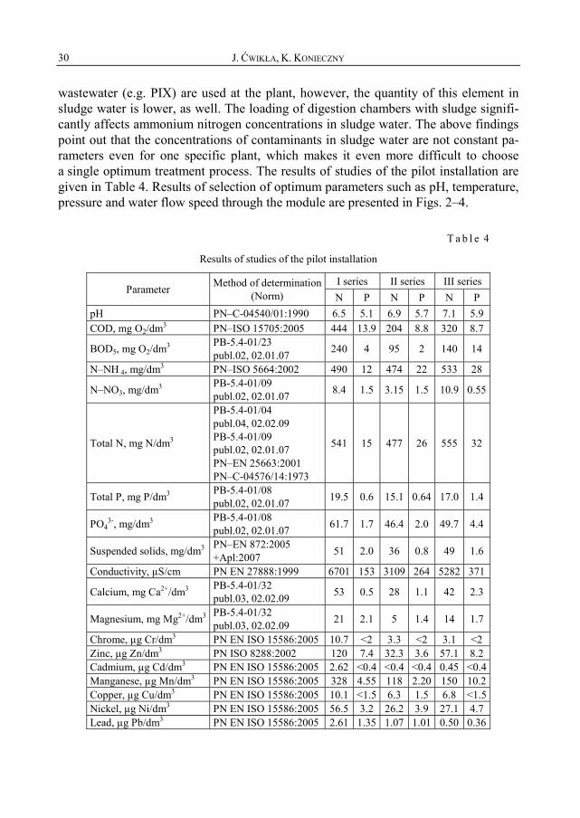
wastewater (e.g. PIX) are used at the plant, however, the quantity of this element in sludge water is lower, as well. The loading of digestion chambers with sludge signifi-cantly affects ammonium nitrogen concentrations in sludge water. The above findings point out that the concentrations of contaminants in sludge water are not constant pa-rameters even for one specific plant, which makes it even more difficult to choose a single optimum treatment process. The results of studies of the pilot installation are given in Table 4. Results of selection of optimum parameters such as pH, temperature, pressure and water flow speed through the module are presented in Figs. 2–4.
T a b l e 4
Results of studies of the pilot installation
Parameter Method of determination(Norm)
I series II series III series N P N P N P
pH PN–C-04540/01:1990 6.5 5.1 6.9 5.7 7.1 5.9 COD, mg O2/dm3 PN–ISO 15705:2005 444 13.9 204 8.8 320 8.7
BOD5, mg O2/dm3 PB-5.4-01/23 publ.02, 02.01.07 240 4 95 2 140 14
N–NH 4, mg/dm3 PN–ISO 5664:2002 490 12 474 22 533 28
N–NO3, mg/dm3 PB-5.4-01/09 publ.02, 02.01.07 8.4 1.5 3.15 1.5 10.9 0.55
Total N, mg N/dm3
PB-5.4-01/04 publ.04, 02.02.09 PB-5.4-01/09 publ.02, 02.01.07 PN–EN 25663:2001 PN–C-04576/14:1973
541 15 477 26 555 32
Total P, mg P/dm3 PB-5.4-01/08 publ.02, 02.01.07 19.5 0.6 15.1 0.64 17.0 1.4
PO43-, mg/dm3 PB-5.4-01/08
publ.02, 02.01.07 61.7 1.7 46.4 2.0 49.7 4.4
Suspended solids, mg/dm3 PN–EN 872:2005 +Apl:2007 51 2.0 36 0.8 49 1.6
Conductivity, μS/cm PN EN 27888:1999 6701 153 3109 264 5282 371
Calcium, mg Ca2+/dm3 PB-5.4-01/32 publ.03, 02.02.09 53 0.5 28 1.1 42 2.3
Magnesium, mg Mg2+/dm3 PB-5.4-01/32 publ.03, 02.02.09 21 2.1 5 1.4 14 1.7
Chrome, μg Cr/dm3 PN EN ISO 15586:2005 10.7 <2 3.3 <2 3.1 <2 Zinc, μg Zn/dm3 PN ISO 8288:2002 120 7.4 32.3 3.6 57.1 8.2 Cadmium, μg Cd/dm3 PN EN ISO 15586:2005 2.62 <0.4 <0.4 <0.4 0.45 <0.4 Manganese, μg Mn/dm3 PN EN ISO 15586:2005 328 4.55 118 2.20 150 10.2 Copper, μg Cu/dm3 PN EN ISO 15586:2005 10.1 <1.5 6.3 1.5 6.8 <1.5 Nickel, μg Ni/dm3 PN EN ISO 15586:2005 56.5 3.2 26.2 3.9 27.1 4.7 Lead, μg Pb/dm3 PN EN ISO 15586:2005 2.61 1.35 1.07 1.01 0.50 0.36

Treatment of sludge water with reverse osmosis 31
It was confirmed that sludge water can be treated by the method of reverse osmo-sis. The process efficiency was very high, as 95% reduction in biogenic compounds was achieved. The reduction level for N and P compounds differed insignificantly according to the feed quality.
Fig. 2. Pressure dependence of the N–NH4 content in permeate
using the Osmonics module and BW 30 membranes; T = 22 °C, flow speed 2 m/s, N–NH4 in feed: 600 mg/dm3
Fig. 3. Dependence of the N–NH4 content in permeate on pH of feed using the Osmonics module and BW 30 membranes;
ΔP = 2 MPa, T = 22 °C, flow speed 2 m/s, N–NH4 in feed 605 mg/dm3

J. ĆWIKŁA, K. KONIECZNY 32
Fig. 4. Dependence of the volumetric flux of permeate on the flow rate through the Osmonics module in the RO process using the BW 30 membrane;
ΔP = 2 MPa, pH = 7.0, T = 22 °C, N–NH4 in feed 590 mg/dm3
The content of ammonium nitrogen in the permeate however, never exceeded 30 mg/dm3, and 1.5 mg/dm3 for general phosphorus, i.e. the permeate composition was similar in this respect to standard urban sewage (Table 4). Additional load brought to the treatment plant with permeate will, therefore, not be significant from the process point of view.
Optimum working conditions for the reverse osmosis were identified: the highest reduction in ammonium nitrogen content was reached for the feed with pH of 6.5 (Fig. 3) under the pressure of 3 MPa. (Fig. 2). However, considering the energy con-sumption and fouling intensity observed for the higher pressure, its the lower value, i.e. 2 MPa was found to be efficient enough to provide satisfactory treatment effect.
A higher intensity of permeate flow was accomplished for feed flowing via the membrane at a lower flow rate (Fig. 4). The reasons would be both turbulent flow for higher flow rate disturbing the convection motion to the membrane and/or torrential growth of flow losses under higher flow rate leading to the decrease of the process driving force.
The concentrate produced in the reverse osmosis was purified by precipitating ammonium and phosphorus compounds in a form of struvite (NH4)Mg(PO4)×6H2O (Table 4). The appropriate amount of magnesium ions and phosphates had to be added to the concentrate for this purpose. It is also important that by concentrating the con-taminants, the tank and the equipment to be used in actual conditions will feature di-mensions and capacities much smaller than when using this technology straightfor-ward for untreated sludge water.
Sedimentation properties of the sludges precipitating from concentrated solutions were better than those of the sludges precipitating from raw sludge water: the

Treatment of sludge water with reverse osmosis 33
precopitates were falling quicker and the occurence of other types of crystals produced in sludges was found in the microscopic image (optical microscope Novex, magnified 40× and 100×). Sludges from the concentrated samples were drying quicker than the those from the samples imitating raw sludge water. Similar reduction values for ammonium nitrogen were obtained from the concentrated and diluted solution. The tests made for actual solutions also differed with regard to the composition of crystals, however, it is necessary to select appropriate process conditions to intensify struvite precipitation considering unsatisfactory reduction in ammonium nitrogen content as compared to the prepared solutions.
Regular, romboidally-shaped crystals along with thin needles and X-shaped forms occured in all the cases. The proportions of various crystal forms in sludges differed, however: forms with regular shapes were prevalent in respect of X-shaped forms for the concentrated solutions and regular forms for the actual solutions were lower in numbers.
The admixtures of other compunds, disturbing the struvite crystallisation process, were probably present in the actual solutions. It is therefore recommened to determine the elemental composition of the sludges produced, which could help to conclude if other crystals than struvite occur in sludges.
The studies have not been completed, yet and they are being continued to produce a series of repeatable results and to select appropriate parameters for the process performed.
6. CONCLUSIONS
The studies have shown that the treatment of sludge water with the reverse osmo-sis method is feasible and its efficiency is very high. The concentrate produced in the process can be treated by the precipitation of struvite sludge. The sludge can be used in agriculture as a good quality fertiliser. The RO module is simple to operate and its installation is resistant to changes in contaminant concentrations in the feed. Breaks in the module usage do not affect the efficiency of the method. There is an opportunity to implement this process for wastewater treatment plants where it can be used for limit-ing the concentration of biogenic loads from external process streams, thereby achiev-ing higher efficiency of nitrogen and phosphorus removal in biological reactors.
REFERENCES
[1] STROUS M., VAN GERVVEN E., ZHENG P., KUENEN J.G., JETTENM S.M., Water Res., 1997, 31 (8), 1955.
[2] CONSTANTINE T., SHEA T., JOHNSON B., Newer approaches for treating return liquors from anaerobic digestion, IWA Spec. Conf. Nutrient Management in Wastewater Treatment Processes and Recycle Streams, Cracow, 2005, 455–464.

J. ĆWIKŁA, K. KONIECZNY 34
[3] CAFFAZ S., LUBELLO C., CANZIANI R., SANTIANNI D., Autotrophic nitrogen removal from anaerobic supernatant of Florence’s WWTP digesters, Newer approaches for treating return liquors from anaerobic digestion, IWA Spec. Conf. Nutrient Management in Wastewater treatment Processes and Recycle Streams, Cracow, 2005, 397–406.
[4] MASŁOŃ A., TOMASZEK J.A., Environ. Prot. Eng., 2007, 33 (2), 175. [5] MALEJ J., MAJEWSKA A., BOGUSKI A., Rocznik Ochr. Środ., 2002, 4, 11. [6] MYSZOGRAJ S., Inż. Ochr. Środ., 2008, 11 (2), 219. [7] BRIDGER G., CEEP Scope Newsletter, 2001, 43, 3. [8] KOŁTUNIEWICZ A.B., DRIOLI E., Membranes in Clean Technologies. Theory and Practice, Wiley,
Weinheim, 2008. [9] MAJEWSKA-NOWAK K., Ochr. Środ., 2007, 2, 21.
[10] KOWAL A., ŚWIDERSKA-BRÓŻ M., Purification of Water, PWN, Warsaw, 2009, p. 311–312 (in Polish).
[11] CHERYAN M., Ultrafiltration and Microfiltration Handbook, Technomic Publ. Comp., Lancaster, 1998. [12] NOWORYTA A., TRUSEK-HOŁOWNIA A., Membrane Separations, Agencja Wyd. ARGI, Wrocław,
2001 (in Polish). [13] NARĘBSKA A., Membrany i membranowe techniki rozdziału, Wyd. Uniw. Mikołaja Kopernika, To-
ruń, 1997. [14] JAFFER Y., CLARK T.A., PEARCE P., PARSONS S.A., Water Res., 2002, 36, 1834.

Environment Protection Engineering Vol. 37 2011 No. 4
WOJCIECH DĄBROWSKI*
RATIONAL OPERATION OF VARIABLE DECLINING RATE FILTERS
An approximate solution to the system of equations governing the flow distribution among vari-able declining rate (VDR) filters results in flow rates through filters being elements of a geometrical progression. Based on this approximation, it was deduced how to operate a plant in order to keep the same flow rates through VDR filters for various total head losses of flow. These principles of opera-tion were carefully verified using the accurate di Bernardo mathematical model of VDR filter plants. It was deduced that the longest filter runs result from such an operation of a plant for which the ratio of the highest to the average flow rates through a filter and simultaneously the affordable total head loss of flow through the plant are the highest.
1. INTRODUCTION
In the forty years since the first application of the variable declining rate (VDR) control system [1], many existing plants have been installed with orifices to replace expensive and sometimes unreliable mechanical flow rate controllers. VDR filters are especially popular in South America, but several water treatment plants using the VDR control system operate successfully in the U.S.A., and in the European Commu-nity.
The idea of declining filtration might be advantageous in further application of ac-tivated carbon, either by itself or as one of filter media layers. A longer time is re-quired for filtration in the case of a clogged activated carbon filter. This longer time facilitates improved adsorption of soluble organic compounds. However, if granular activated carbon (GAC) filters follow conventional sand or sand–anthracite filters the GAC media often requires backwashing to avoid high bacteriological content in fil-trate, before any significant clogging of carbon is observed [2]. So far it is difficult to
_________________________ *Water Supply and Environmental Engineering Institute, Cracow University of Technology,
ul. Warszawska 24, 31-135 Cracow, Poland, e-mail: [email protected]

W. DĄBROWSKI 36
judge how effectively the VDR system of operation will compete with mechanical flow controllers, as this second type of a flow control system can also be constructed to operate under a declining flow rate in a more manageable fashion than that offered by orifices installed at the outflows from the filters. However, it is evident that vari-able declining rate (VDR) filters are an economically reasonable solution for all treat-ment plants unable to meet the water quality demands or those poorly controlled. Moreover, it has been shown several times that the quality of filtrate produced by fil-ters operated under this system is at least as good as that obtained under a constant filtration velocity [3–8]. Thus, it is easy to understand why this invention has spread rapidly in countries where increasing water demands exist but still low financial capa-bilities. VDR filters offer some advantages as an increase in plant capacity, longer filter runs or a decrease in the total head loss in the system. If only one of these factors is chosen for maximization, it limits or excludes making use of other opportunities. Therefore, a proper design of a VDR filter system is best approached as an optimisa-tion problem.
Optimisation theory is a powerful tool which deals with hundreds or even thou-sands of decision variables, especially when linear problems are concerned. In the case of retrofitting a plant with a VDR filter control system there are only a few operation parameters to be optimised. Therefore major difficulty results from a lack of compre-hensive knowledge about relations existing between them. However, there are several prospective methods of computing hydraulic control systems of VDR filters. An ap-proximate solution to di Bernardo’s [9, 10] mathematical model is used here to elabo-rate several relationships between filters operating in a bank. Most of these relation-ships have been found to be useful in an optimisation procedure proposed for the hydraulic control system of a VDR filter plant. It was assumed that an existing water treatment plant is equipped with hydraulic flow rate controllers (orifices) located at the outflow pipe from each of the filters [10, 11]. The maximum available head loss, the ratio of the maximum to the mean flow rate, the flow rate through the whole plant and the filter media are assumed to be fixed. The coefficients characterizing the friction created by orifices, the ratio of maximum qmax to average qavr flow rates through the filter units, the height of water surface fluctuation above filter media h0, and the value of the total head loss of flow through the system H are decision variables. The goal is to minimize the frequency of backwash subject to the constraints imposed on the deci-sion variables by the total plant capacity, affordable head loss of flow through the system, and the highest admissible flow rate through a clean filter.
2. FLOW CONTROL SYSTEM
Variable declining rate filters are equipped with identical orifices installed at in-flows or outflows from all filters. The operation of such a filter plant is based on co-

Rational operation of variable declining rate filters 37
operation between head losses created by linear laminar flow through filter media with head loses of turbulent flow through orifices and transitional flow through the drain-age [11, 12]. The operational parameters of the flow control system should be selected in such a way to restrict flow through the freshly backwashed filters mostly by head losses of flow through orifices. However, for the most significantly clogged filter, waiting for backwash, this head loss should be negligible in comparison with the head loss of flow through the filter media. The principles of the VDRF plant operation are described elsewhere [10–18]. The following assumptions were made:
• there are at least four filters in a bank, • all filters are identical, • inflows are located below the lowest water surface above the filter media, • head losses in piping are negligible in comparison with those created by filter
media, • orifices are located at outflows from filters.
Fig. 1. The place of installation of an orifice:
1 – air, 2 – raw water, 3 – wastewater, 4 – backwash water, 5 – filtrate, 6 – orifice
Under these assumptions the unconfined water surface level is the same above all filters in any moment of time. This level rises in time due to clogging of filter media, to drop down quite rapidly after restoring the most recently backwashed filter to service. The place of installing orifices controlling flow rates through filters is presented in Fig. 1. Examples of patterns of water and flow rates are presented in Figs. 2, 3.

W. DĄBROWSKI 38
Fig. 2. An example of water table fluctuations at the pilot VDR filter plant
constructed at the Cracow University of Technology
Fig. 3. An example of flow rates recorded at the pilot VDR filter plant constructed at the Cracow University of Technology
3. EQUATIONS
Di Bernardo [9, 10] proposed a model of the variable declining rate filter control system under the following assumptions:
1. All flow rates vary only at time of and just after a backwash of one filter, thus they remain essentially constant between subsequent backwashes in a plant.
2. The period of a backwash of one of the filters is so short that the hydraulic re-sistances of the filters remaining in service are not visibly affected by clogging during this period (the resistance of a filter i is recognized to be the same before and after the backwash of a filter z).
Di Bernardo [9, 10] compared theoretical results obtained by his model with ex-perimental data collected from a pilot plant as well as from a full-scale filtration plant and he received strong support for his theory. Dąbrowski [11] found the Di Bernardo model to give results similar to those produced from the set of equations elaborated by

Rational operation of variable declining rate filters 39
Arboleda et al. [16] and summarized di Bernardo’s model in a set of z + 1 Eqs. (1)–(3). Mackie et al [12] proved the solution to the system of Eqs. (1)–(3) to be close to results of computations based on the unit bed element (UBE) [19] model of a filter plant
• z – 1 equations
0 2 1 2
1
n ni i
i i
H h c q H c qq q
+
+
− − −= (1)
• 1 equation
( )0 1 1 2 1 nH h c q c q− = + (2)
• 1 equation
1
i z
ii
Q q=
=
=∑ (3)
where: c1 is a proportional coefficient characterizing the resistance of clean medium, c2 – coefficient of turbulent head losses, H – total head loss of flow through the plant just before a backwash, h0 – height of water surface increase between backwashes, i – number of a filter in a bank, n – exponent of turbulent and transitional head loss created by orifices and drainage, qi – flow rate through ith unit, qi = q1 for i = 1, etc., Q – total flow rate through the system, z – number of filters in a bank.
Equations (1) does not account for compressing of deposit in filter media, which is an easily visible phenomenon in the case of increasing [20] and less visible for de-creasing [21] of coagulated water suspension filtration velocity. However, extensive pilot plant experiments [22] proved that the di Bernardo model [10] was surprisingly accurate for modelling filter plants following chemical pretreatment and flocculators. There are (z – 1) equations (1) and two single Eqs. (2), (3) where z is the number of filters in a bank.
Three approximate solutions to the system of Eqs. (1)–(3) were elaborated [11] and tested in comparison with accurate numerical solutions and with experimental data. Approximation (4) to Eq. (1) was definitely of the worst accuracy but still gave quite acceptable results:
1 01i
i
q hq H
+ = − (4)
According to this approximation flow rates through filters are elements of a geo-metrical progression. Obviously approximated Eq. (4) to Eq. (1) may be applied only as long as the parameters of a filter plant operation H, h0, z, c1, c2, q1 ..., qi ..., .qz are in the range commonly used in water filtration practice. Beyond this range the substitu-tion of Eq. (1) by Eq. (4) may result in unexpectedly high errors of calculations.

W. DĄBROWSKI 40
4. BASIC RULES
Some general properties of VDR filters developed from a solution to the set of Eqs. (2)–(4) give an idea which particular parameters should be considered in optimi-sation of filter runs. Since Eq. (4) is a rough approximation to Eq. (1), thus all the con-clusions developed here were carefully verified in numerical experiments by rigorous solution to the set of Eqs. (1)–(3). The theory developed here is limited to a recon-struction of an existing plant, so the coefficient c1, describing the hydraulic resistance of a clean porous medium against the flow, is given. The head loss H, height of water table fluctuations over the filters h0, and the turbulent head loss coefficient c2 are ad-justed in calculations to meet the required optimisation goals. However, prior to for-mulation of the optimisation problem, some properties of the solution to the system of Eqs. (2)–(4) are summarized. These properties will be used later in search for a special family of solutions to the set of Eqs. (1)–(3) for which flow rates through filter units remain almost the same when parameters of a filter plant operation change according to basic rules defined in the next paragraph.
5. PROPERTIES OF THE SOLUTION TO THE SYSTEM OF EQUATIONS (2)–(4)
Prior to formulation of the optimisation problem, some properties of the solution to the system of Eqs. (2), (3), (4) are summarized. Property 1 follows directly from Eq. (4).
Theorem 1. The ratio of qi+1/qi does not depend on the number i of a filter in a bank. If the values of H and h0 are the subject of change in such a particular way that h0/H is the same each time the ratio qi+1/qi remains constant.
From this statement and from Eqs. (2), (3) a practical rule for management of VDR control systems may be directly deduced.
Theorem 2. In order to receive the same flow rates through all filters in a plant q1, ..., qi, ..., qz for any feasibly chosen new values of the total head loss of flow through a plant before a subsequent backwash H, parameters of the plant operation c2, h0 should be adjusted according to the following rules:
1) h0 is to be calculated for a new value H directly from a constant (equal to the previous) value of the quotient h0/H.
2) The coefficient characterizing the orifice c2 is to be calculated from Eq. (2) in order to give the same q1.
Finally, a whole family of solutions to the set of Eqs. (2)–(4) characterized by the same total plant capacity Q and the same flow rates qi through all filters is obtained.

Rational operation of variable declining rate filters 41
Such a family of solutions is presented in Fig. 4 based on a rigorous numerical solu-tion to the system of Eqs. (1)–(3) supplied with the same data c1, Q, z, n as given in di Bernardo’s [9, 10] example of calculations for a pilot plant – see Table 1. In these computations, the ratio of q1/qavr was imposed to be equal to 1.3. The flow rates now refer to 1 m2 of a filter (hydraulic load), so consequently, the following dimensions are in use: H [m H2O], q [m/day], Q [m/day], c1 [(m H2O)/(m/day)], c2[(m H2O)/(m/day)n].
T a b l e 1
Coefficients c1, c2, n of Eq. (2) measured by Di Bernardo [9], [10] for a pilot and a full scale plantsa
Scale of the plant
Numberof filters
c1
[(m H2O)/(m/day)]c2
[(m H2O)/(m/day)n] n
Pilot plant 4 0.00145 0.00050 1.22Full scale plant 4 0.00150 0.0000026 1.90
aThe coefficients c1, c2 were predicted for qi referred to 1 m2
(hydraulic load, [m3/(m2·day)] simplified to [(m/day)]). The curves qi(H) in Fig. 4 fit perfectly with the horizontal straight lines expected
here in spite of the fact that they are not received from the rough approximation (4), but from the precise numerical solution [11] to the set of Eqs. (1)–(3). Fifty different values of H were chosen, then h0, c2 calculated according to the points 1, 2 of the theo-rem 2 and finally qi computed from the system of Eqs. (1)–(3). The set of Eqs. (1)–(3) was solved by the most precise of the methods described elsewhere [11]. In this method, each value of qi is bounded both from the upper and the lower side but these limits are so close to each other that they are denoted by single lines in Fig. 4.
Fig. 4. Distribution of the flow rate vs. H for a family of solutions calculated
according to property 1 for Q = 704 m/day, q1/qavr = 1.3, and for the same data c1, n as for the pilot plant experiments (Table 1 after [9, 10])
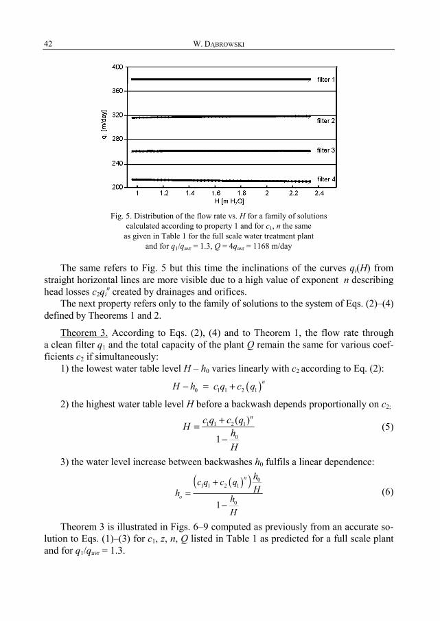
W. DĄBROWSKI 42
Fig. 5. Distribution of the flow rate vs. H for a family of solutions
calculated according to property 1 and for c1, n the same as given in Table 1 for the full scale water treatment plant
and for q1/qavr = 1.3, Q = 4qavr = 1168 m/day
The same refers to Fig. 5 but this time the inclinations of the curves qi(H) from straight horizontal lines are more visible due to a high value of exponent n describing head losses c2qi
n created by drainages and orifices. The next property refers only to the family of solutions to the system of Eqs. (2)–(4)
defined by Theorems 1 and 2.
Theorem 3. According to Eqs. (2), (4) and to Theorem 1, the flow rate through a clean filter q1 and the total capacity of the plant Q remain the same for various coef-ficients c2 if simultaneously:
1) the lowest water table level H – h0 varies linearly with c2 according to Eq. (2):
( )0 1 1 2 1 nH h c q c q− = +
2) the highest water table level H before a backwash depends proportionally on c2;
1 1 2 1
0
( )
1
nc q c qH hH
+=−
(5)
3) the water level increase between backwashes h0 fulfils a linear dependence:
( )( ) 0
1 1 2 1
01
n
o
hc q c qHh h
H
+=
− (6)
Theorem 3 is illustrated in Figs. 6–9 computed as previously from an accurate so-lution to Eqs. (1)–(3) for c1, z, n, Q listed in Table 1 as predicted for a full scale plant and for q1/qavr = 1.3.

Rational operation of variable declining rate filters 43
Fig. 6. Total head loss H as a function of c2 for data presented in Fig. 5
Fig. 7. Head loss H as a function of c2 (for c1, n as for the full scale treatment plant
reported in Table 1) in comparison with the head loss computed for more filters operating with the same qavr = Q/z = 292 m/day, q1/qavr = 1.3
Fig. 8. The highest water table fluctuation h0 over the filters, computed
as a function of c2 for the same data as the calculations presented in Fig. 5

W. DĄBROWSKI 44
Fig. 9. Head loss H – h0 calculated as a function of c2 for the same data as in Figs. 5, 6
The next theorem refers to the resistance of hydraulic porous media c1z to flow just before its backwash. As the total head loss of flow through the plant is equal to H just before each of backwashes, c1z is defined by:
( )1 2 nz z zH c q c q= + (7)
Equation (7) is introduced for the most clogged filter z operated with the flow rate qz.
Theorem 4. For a family of solutions to the set of Eqs. (2)–(4) constructed accord-ing to the points 1, 2 of Theorem 2 (so characterized by the same values of flow rates q1, ..., qi, ..., qz) the hydraulic resistance c1z of the most clogged filter media just before its backwash depends linearly on the constant c2 being proportional to the turbulent head losses in the drainage and orifices:
0
1 1 2 1 2
10
1
1
n nz
z
z
hc q c q c qHc
hqH
⎛ ⎞+ − −⎜ ⎟⎝ ⎠=
⎛ ⎞−⎜ ⎟⎝ ⎠
(8)
The family of solutions to the system of Eqs. (4), (2), (3) calculated according to the instructions given by Theorems 1–3 have almost identical flow distribution q1, ..., qi ..., qz between filters in a bank and a constant ratio h0/H. Equation (8) results directly from the definition of c1z (7) and from Eqs. (2), (6). Theorem 4 is illustrated in Figs. 10, 11 constructed as previously from fifty accurate solutions to the set of Eqs. (1)–(3). The data for these computations are the same as those listed in Table 1, with q1/qavr = 1.3 in this instance. It may be seen that the resistance c1z is almost a lin-ear function of c2. However, the ratio of c1z/H as a function of c2 shows some unlinear-ity as presented in Fig. 12, constructed from the solutions to the system of Eqs. (1)–(3) for 50 different values of c2.

Rational operation of variable declining rate filters 45
Fig. 10. Relative resistance c1i/c1 of four filters before backwashing
calculated as a function of c2 for Q = 704 m/day, q1/qavr = 1.3, and for c1, n the same as for the pilot plant (see Table 1) ; the most clogged filter 4
Fig. 11. Resistance of four filters as a function of c2 for the same n, c1 as for the full scale plant reported in Table 1, and for q1/qavr = 1.3, Q = 4qavr = 1168 m/day
Fig. 12. Some nonlinearity of the ratio c1z/H as a function of c2 according to computations based on a precise numerical solution to the system of Eqs. (1)–(3)
and subject to the same Q, q, c1, n as for Figs. 5–9, 11

W. DĄBROWSKI 46
6. OPTIMISATION PROBLEM
It is assumed that the highest resistance of porous media to flow corresponds to the largest volume of water passing through a filter. This usually reasonable assump-tion is not always valid as the depth bed filtration theory gives a complex picture of the head loss increase with time and filtration velocity impacts a pattern of deposit distribution in depth. However, in most optimisation tasks it is not possible to avoid some simplifications. It is believed that the substitution of a problem on the longest filter run by the problem on the highest media resistance to flow c1z at the end of this run is acceptable in many technical applications. Concluding the objective function is defined by the equation
21Max
nz
zz
H c qcq−= (9)
The constraints include the set of Eqs. (4), (2), (3) and some limits imposed to the total available head loss of flow H and the ratio of flow rate q1 to the average flow rate qavr:
H ≤ Hmax (10)
1
avr
q Dq
≤ (11)
where: Hmax – the highest available head loss of flow through a plant limited by its construction, D – limit imposed on the ratio q1/qavr because of required filtrate quality.
The formulated optimisation problem will be solved in two steps. First it will be shown that for all families of solutions to the set of Eqs. (4), (2), (3) characterized by flow rate distribution q1, ..., qi, ..., qz for which q1/qavr = D the highest hydraulic resis-tance to flow of the most clogged filter c1z, just before its backwash, refers to the high-est coefficient c2. For this value of c2 the total head loss of flow through the plant H reaches Hmax. In the latter step, it will be proved that any solution being outside of these families of solutions for which q1/qavr = D refers to a lower value of c1z, than received simultaneously for q1/qavr = D and for H = Hmax.
7. SOLUTIONS
The solution to the optimisation problem inside of the family of fixed values of q1, ..., qi, ..., qz, for which q1/qavr = D results directly from theorems 1–4. As the pa-rameters c2, H, h0 have to be adjusted through Eqs. (2), (5), (6) resulting in the re-quired Q, q1/qavr, the same h0/H and qz, so the resistance of the filter media z in Eq. (8) linearly depends on c2 and is the highest for the value of c2 for which H = Hmax. This might be intuitively expected.

Rational operation of variable declining rate filters 47
The family of solutions defined by the points 1–3 fulfilling Theorem 3 refers to the highest acceptable value of q1. There are also solutions to the set of Eqs. (4), (2), (3) fulfilling constrains (10), (11) but not belonging to this family. These solutions satisfy required plant capacity Q for some lower values of the largest flow rate *
1 ,q and for different flow rate distributions * * *1 , ..., , ...,i zq q q among the filters. To
make this text clear, the same notations are used as previously to describe h0, q1, ..., qi, ..., qz, c2, c1z when they refer to the solutions of the set of Eqs. (4), (2), (3) being a sub-ject to the restriction q1/qavr < D, and not belonging to the family of fixed q1, ..., qi, ..., qz, for which q1/qavr = D. However, in this case they are denoted additionally by an asterisk, thus *
1 1.q q< As the filter media is known in advance and all comparisons between the results of calculations will be done for the same arbitrarily chosen head loss H before a subsequent backwash in a plant, there is no reason to use the asterisk * to distinguish c1 and H for separate families of solutions.
Let us take into account two different solutions to the system of Eqs. (4), (2), (3), both satisfying the same plant capacity for the same available head loss H. The second of these solutions * * * * *
1 2 0, ..., , ..., , ,i zq q q c h refers to 1< q1/qavr < D. At the end of a filter run, the resistance of the most clogged porous media may be described by the equa-tion:
* *
* 2 21 1*
( ) ,n n
z zz z
z z
H c q H c qc cq q
− −= = (7*)
We shall investigate the relations between c2, qz, and * *2 , zc q in advance to confront c1z
with *1 .zc For further discussion it is useful to have a closer look at the relations between
h0, H – h0 and * *0 0, .h H h− According to approximation (4) both flow rate distributions q1,
...,qi, ...,qz and * * *1 , ..., , ...,i zq q q consist of elements of geometric progression giving an
identical plant capacity Q = q1 + ... + qi + ... + qz = * * *1 ... ... .i zq q q+ + + + Bearing in mind
that by definition the flow rate *1q is lower than q1 obviously *
zq must be higher than qz. Moreover from Eq. (4) *
0 0, .h h< As both solutions (with and without the asterisk) refer to the same available head loss H, thus *
0 0 ,H h H h− > − which means that the turbulent
head loss coefficients c2 and *2c fulfil the inequality ( ) ( ) * * *
1 1 2 1 1 1 2 1 .n nc q c q c q c q+ > +
Keeping in mind that from the definition of q1 any value of *1q is lower than q1, it is
obvious that *2 2.c c> All the necessary items of information on the relations between
* *2 2, and ,z zc c q q have been collected * *
2 2( , ),z zc c q q> > and finally the expectation that *1zc is lower than c1z may be confirmed by discussing the equation:

W. DĄBROWSKI 48
1 * * * 11 2 1 2*( ) , ( )n n
z z z zz z
H Hc c q c c qq q
− −= − = − (7**)
Concluding, the highest hydraulic resistance of filter media before backwashing should be sought among the family of solutions q1, ... qi, ... qz, c2, h0, subject to q1/qavr = D. Finally, the highest value of c1z (and hopefully the longest filter run) refers to H = Hmax and to q1/qavr = D.
8. PRACTICAL ASPECTS
A possible application of equations and theorems discussed here is now presented in an optimisation example calculated for a four-filter plant. The conditions assumed are those of di Bernardo [9, 10] for a full scale plant (see Table 1): According to the theorems developed in the previous paragraphs, the highest resistance of the media before a backwash occurs if simultaneously the ratio of q1/qavr and H reach their maximum values.
Fig. 13. The ratio of c1/c1z as a function of H and q1/qavr for an optimisation example
Fig. 14. Values of h0/H as a function of q1/qavr and to some extent also a function of H (data the same as for Fig. 11)

Rational operation of variable declining rate filters 49
Usually q1/qavr is limited by technological reasons and H mainly by the construc-tion of a plant. This simple optimisation rule was tested many times in numerical cal-culations. Examples of such tests are presented in Figs. 13 and 14. Each of lines in these figures was constructed from 50 points obtained from an accurate numerical solution to the set of Eqs. (1)–(3). A full system of equations was used again to verify the optimisation approach developed based on the approximated model described by the set of Eqs. (4), (2), (3). Coefficients c1, n and the plant capacity are the same as in di Bernardo’s [10] full scale experiments. Values h0, c2 were adjusted in such a way that the same Q and q1/qavr were obtained for different values of H varying from 1.2 to 2.5 m. From Figure 13 it can be seen that the resistance of the filter media z increases as q1/qavr increases (for the same H) and behaves analogously if H increases for the same q1/qavr . The value of h0/H remains almost constant for all computations referring to the same q1/qavr (Fig. 14).
9. CONSTANT VERSUS VARIABLE RATE FILTRATION
To evaluate the advantage resulting from using the VDR control system, as op-posed to the constant flow rate system, two filter plants consisted of z = 4 identical filter media, producing the same amount of filtrate, and operated with the same total head loss H were compared. The ratio of c1z (CRF)/c1z(VDRF) was calculated and shown in Fig. 15.
Fig. 15. Ratio of the filter media resistances before a backwash c1z (CRF)/c1z(VDRF), representative of Constant rate and variable declining rate filter operation, respectively
Here c1z(CRF) presents the hydraulic resistance of the constant rate filter (CRF) media z just before the backwash and c1z(VDRF) resistance of the variable declining rate filter (VDRF) media z. The resistance c1z(CRF) was calculated as equal to (H – 0.2 m)/qavr, on the assumption that the head loss of flow through the filter drain-age and an open flow rate controller (at the end of the filter run) is equal to 0.2 m H2O.

W. DĄBROWSKI 50
For q1/qavr = 1.1 the resistance of the clogged filter media is usually higher in a CFR system than it is in a VDR one. Therefore it is possible that no profit would result from VDR control system and these results are not included in Fig. 15. For q1/qavr = 1.2 VDR control system results in higher hydraulic resistance c1z of filter media z for H < 2.0 m. Higher the ratio q1/qavr, lower the ratio c1z(CRF)/c1z(VDRF) is and more profitable is the VDR operation system. However, the ratio q1/qavr is to be restricted because of the filtrate quality. A limit of 1.3 or more commonly 1.5 is imposed on this ratio on a rule of thumb but pilot plant experiments should be used to verify these limits for a given case. In such pilot experiments particles counting is much more reliable than turbidity measuring.
10. THE MOSTLY CLOGGED FILTER
Till now only the maximum ratio of q1/qavr was concerned as a significant factor of the filtrate quality to be determined experimentally. However, the turbidity of filtrate produced by the dirtiest filter may be of crucial concern. The product hmediaq is some-times recognized as a representative parameter for filtrate quality relating to given raw water, pretreatment, and porous media. By hmedia head loss created by filter media is created. The flow rates qz (four filters) obtained according to precise solution to the set of Eqs. (1)–(3) are denoted by circles in Fig. 16 in comparison with a monogram qz/qavr constructed as a function of h0/H from Eq. (12):
( 1)0
avr 0 0
1
1 1
z
zz
hzq Hq h h
H H
−⎛ ⎞−⎜ ⎟⎝ ⎠=⎛ ⎞⎛ ⎞− −⎜ ⎟⎜ ⎟
⎝ ⎠⎝ ⎠
(12)
resulting directly from approximation (4) and from the formula for a sum of geometri-cal progression elements q1 ..., qi ..., qz. The general monogram can be applied to any VDR water filtration plant but it is based on rough approximation (4), so the points denoted by circles do not lay exactly on the line developed for a four filter plant. Each of these points represents a value of qz/qavr computed from the set of Eqs. (1)–(3) for tests in which q1/qavr = 1.1, 1.2, 1.3, 1.4 and 1.5. For these particular tests qz versus h0/H are presented in Fig. 16. If for instance a total available head loss H in this plant is equal to 2.2 m, h0 = 0.61 m, and q1 = 438 m/day = 1.5qavr was chosen experimen-tally it is advisable to verify also the quality of filtrate collected from the mostly clogged filter (c1z = c1/0.12, see Fig. 13) operated with qz = 0.58qavr = 0.58q1/1.5 = 169 m/day (Fig. 16). If the filtrate quality is poor, it is a question of economy whether it is reasonable to improve pretreatment or whether a lower H, rather than the maximum available value, should be considered. In general, optimising of chemical

Rational operation of variable declining rate filters 51
treatment should be attempted first as it has usually a tremendous impact on both fil-tration quality and length of a filter run.
Fig. 16. Monogram for primary values qz in comparison with some points obtained from an optimisation example
Fig. 17 Almost constant values of qz versus H calculated for an optimisation example
11. FINAL REMARKS
The theorems presented in the paper and the optimisation approach to operation of a VDR filter plant were developed from the set of Eqs. (4), (2), (3) but verified by numerical solutions to the set of Eqs. (1)–(3), which does not include a simplified Eq. (4). The data from a pilot and a technical scale treatment plants reported by di Bernardo [9, 10] were used for verification of the findings. However, this verifica-tion is still limited and partially numerical, so a pilot plant was constructed at the Cra-cow University of Technology [24] to carry out empirical tests. The results of experi-ments confirming the theory presented here and advantages of application of the optimisation approach to both a pilot and a full-scale treatment plants will be de-scribed in the next paper.
W. DĄBROWSKI 52
12. CONCLUSIONS
Approximation (4) has been found to be useful in deducing some approximate lin-ear relationships between the parameters of a VDRF hydraulic control system. Based on this approximation, it has been shown that the highest resistance of filter z media before backwashing is related to the highest available head loss of flow through a plant and to the turbulent resistance of orifices adjusted to obtain as high a flow rate through a clean filter as technologically possible. The deduced properties of the solu-tion to the system of equations governing VDR filter plants have been verified in comparison with numerical solutions, which in turn have been compared with litera-ture experimental data.
It is expected that the longest duration of filter runs is related to the highest resis-tance of the filter media just before the backwash. In conclusion, the theoretical con-siderations presented here led to a more efficient filter plant operation method based on an increase of both the water table level above filter media and the ratio of maxi-mum to average flow rates to the highest acceptable values.
Perhaps the best solution to optimisation problems is a pilot plant experiment tak-ing into consideration some of the linear relations developed in the present paper (Theorems 1–4). Such a pilot plant and calculations would have to take into account any possible changes in the water temperature in summer and winter [25].
SYMBOLS
c1 – proportional coefficient characterizing the resistance of a clean medium c2 – coefficient of turbulent head losses c1z – resistance of filter media z before a backwash c1z(CRF) – resistance of filter media z for constant flow rate control system D – constant value H – total head loss of flow through the plant just before a backwash hmedia – head loss of flow through filter media just before its backwash h0 – the height of water surface increase between backwashes i – number of a filter in a bank n – exponent of turbulent head loss Q – total flow rate through the system qi – flow rate through a filter i qavr – mean value of flow rate through a filter qavr = Q/z z – number of the filters in a bank
ACKNOWLEDGEMENTS
This work was sponsored by the Polish National Foundation as a part of the project 1235/T09/2005/28.

Rational operation of variable declining rate filters 53
REFERENCES
[1] CLEASBY J.L., J. Am. Water Works Assoc., 1969, 61 (4), 181. [2] DĄBROWSKI W., ZIELINA M., KUŁAKOWSKI P., SPACZYŃSKA M., Evaluation of sorption into granular
activated carbon by UV absorbance, 5th Int. Conf. Hydro-Science and Engineering, September 18–12 2002, Warsaw, on CD.
[3] DI BERNARDO L., CLEASBY J.L., J. Environ. Eng. Div., 1980, 106, 1023. [4] HILMOE D.J., A comparison of constant rate and declining rate direct filtration of a surface water
supply, Thesis presented to Iowa State University, in partial fulfilment of the requirements for the MSci. degree, 1983.
[5] HILMOE D.J., CLEASBY J.L., J. Am. Water Works Assoc., 1986, 78 (12), 26. [6] CLEASBY J.L., Water Sci. Technol., 1993, 27 (10), 151. [7] MACKIE R.I., DĄBROWSKI W., ZIELINA M., Environ. Prot. Eng., 2007, 33 (4), 27. [8] CORNWELL D.A., BISHOP M.M., DUNN H.J., J. Am. Water Works Assoc., 1984, 76 (12), 55. [9] DI BERNARDO L., A rational method to the design of declining rate filters, 4th World Filtration Con-
gress, Ostend, Belgium, 1986 (manuscript). [10] DI BERNARDO L., Filtration Separation, 1987, Sept./Oct., 338. [11] DĄBROWSKI W., Acta Hydroch. Hydrob., 2006, 34 (5), 442. [12] MACKIE R.I., DĄBROWSKI W., ZIELINA M., Environ. Prot. Eng., 2003, 29 (1), 45. [13] AKGIRAY O., SAATÇI A.M., Water Sci. Technol., 1998, 38(6), 89. [14] SAATÇI A.M., J. Environ. Eng., 1989, 115 (2), 462. [15] CHAUDHRY F.H., J. Environ. Eng., 1987, 113 (4), 852. [16] ARBOLEDA J., GIRALDO R., SNEL H., J. Am. Water Works Assoc., 1985, 77 (12), 67. [17] CLEASBY J.L., DI BERNARDO L., J. Environ. Eng. Div., 1980, 106,1043. [18] DROŻDŻ J., Gaz, Woda i Technika Sanit., 1979, 55 (4), 108. [19] MACKIE R.I., ZHAO Q., Water Res., 1999, 33 (3),794. [20] DĄBROWSKI W., A discussion of controversies regarding deep bed filtration for water treatment,
Filtech – Int. Conf. Exhibition for Filtration and Separation Technology, 2005, 11–13 October., Rhein-Main-Hallen Wiesbaden, Germany, Vol.1, I-394–401.
[21] DĄBROWSKI W., Arch. Hydro-Eng. Environ. Mechanics, 1993, 40 (1/2),135. [22] ZIELINA M., Theoretical and Empirical Investigations into Water Rapid Filters of Variable Declining
Rate, Thesis presented to the Environmental Engineering Department, Cracow University of Tech-nology, in the partial fulfilment of the requirements for the degree of PhD, Cracow, 2002.
[23] ZIELINA M., DĄBROWSKI W., MACKIE R.I., Empirical verification of an optimisation approach to a VDR filter plant operation, 5th Int. Conf. Hydro-Science and Engineering, 1992, September 08–12, Warsaw (on CD).
[24] ZIELINA M., DĄBROWSKI W., Principles of Designing and Operating Rapid Filter Plants Which Are Not Supplied with Flow-Rate Regulators, Monograph 293, the Cracow University of Technology, 2003, Cracow (in Polish).
[25] DĄBROWSKI W., MACKIE R.I., Arch. Hydro-Eng. Environ. Mechanics, 1994, 41 (3–4), 37.


Environment Protection Engineering Vol. 37 2011 No. 4
WOJCIECH GOLIMOWSKI*, AGNIESZKA GRACZYK-PAWLAK*
INFLUENCE OF ESTERIFICATION OF WASTE FATS PROCESS PARAMETERS ON AGRICULTURAL
BIOFUEL PRODUCTION FACILITIES
The paper presents the influence of esterification process parameters in waste fats on their level of reaction. Raw materials contained: frying rapeseed oil, animal lard, methyl alcohol and potassium hydroxide as a catalyst, necessary for reaction in non-pressure conditions. Esterification was carried out at 35–40 °C and 60–65 °C in two separate esterificators differing from one another with mixing systems. It has been established that in terms of contents of non-reactants allowed the obtained prod-uct meets the European EN 14214 standard, determining the quality of biodiesel.
1. INTRODUCTION
In search of alternative fuels, Szlachta [1] pointed at methyl esters of higher fatty acids, their properties being close to those of motor oil. In the nineties, a research was conducted in Poland on capabilities to produce biofuels by farmer producers out of raw rapeseed oil [2], based on the technology of low-temperature transesterifica-tion [3]. From the moment of publishing the information on a prototype low-efficiency installation for fuel production [4], there has been an increasing interest among far-mers. In 2007, a rapid increase in rape prices [5] along with a decrease in oil prices caused the farmers to seek other inexpensive sources to produce methyl esters.
Walisiewicz-Niedbalska and Podkówka [6] proposed to utilize frying oils and an-imal fats for biofuels production for own use. Research conducted by Sulewski et al. [7], Wang et al. [8], Leong et al. [9], Predojević [10], Phan [11] have shown that me-thyl esters from frying oils from various sources have similar properties. Animal fats are solid at room temperature due to high content of saturated fatty acids [12]. As shown in the studies performed by Tashtoush et al. [13], Wyatt’a et al. [14], Goli-moski and Nowak [15] biofuels made from animal fats as well as frying oils have sim- _________________________
*Institute of Technology and Life Sciences, Poznań, ul. Biskupińska 67, 60-463 Poznań, Poland; corresponding author W. Golimowski, e-mail: [email protected]

W. GOLIMOWSKI, A. GRACZYK-PAWLAK 56
ilar properties as diesel fuel, except for their freezing point, which takes positive val-ues. Biodiesel, based on frying oil, is manufactured on industrial scale in Austria, where it contributes to 1.5% of fuel’s national supply [16]. In Denmark, the Daka company produces biodiesel from animal fats [17].
The analyses of waste fats-based biofuel properties performed so far, in most cases did not determine the presence of free glycerol and unreacted particles. According to Stren-ziok and Wickboldt [18], an excessive presence of these particles can cause serious dam-age to the engine. A research conducted by Golimowski et al. [19] on the production of biofuels based on low-temperature esterification technology from refined rapeseed oil as well as from fresh animal lard, has shown increased participation of di- and triglyceride in the ester phase. This proves low reaction level of triglycerides.
The study aimed at evaluating the influence of the reaction environment and the kind of raw materials on the occurrence of glycerol groups in methyl esters of higher fatty acids. Present knowledge provides no information on the quality of waste fat-based biofuels, manufactured in homesteads for own use.
2. MATERIALS AND METHODS
Raw materials used in the research were waste rapeseed oil (FO) and animal lard (AL), which went rancid on behalf of bad storage. Substrates necessary for esterifica-tion were methyl alcohol with molar part of 6 to 1 and a 2% addition of potassium hydroxide. 8 kg of raw materials were used for one trial.
T a b l e 1
Physical and chemical properties of materials used
Parameters FO AL Acid value, mg KOH·g–1 2.6 7.3 Thickness at 20 °, kg·m–3C 912 915 Kinematic viscosity at 40 °C, mm2·s–1 53.99 42.63Combustion temperature, °C 242 244 Calorific value, MJ·kg–1 38.9 39.1
Physicochemical properties of the materials were described and compared to those
of food fats. The results obtained are given in Tables 1 and 2. In the next stage of the study, frying oil and animal fats underwent the esterification process, which was car-ried out in two separate esterificators: hydraulically mixed (EH) and mechanically mixed (EM) at 35–40 °C and 60–65 °C after mixing the substrates for 30 minutes. Post-reactive product was placed in sedimentation columns for 24 h, where it distri-buted into two phases: ester phase and glycerol phase. After two weeks, the concentra-

Agricultural biofuel production facilities 57
tion of unreacted particles and free glycerol in the ester phase was determined using the gas chromatography (Clarus 600, PerkinElmer). The measurement was performed in accordance to the Polish standard PN-EN 14105, regarding free and total glycerol and mono-, di-, triglycerides.
T a b l e 2
The contribution of fatty acids [%]
Fatty acids Systematic nameof the acid Carbon number
Measurement results Rapeseed oil [20]
Lard [21] FO AL
Saturated
tetradecanoic 14:0 – 2.28 0.06 0.58 pentadecanoic 15:0 – 0.25 – – hexadecanoic 16:0 5.45 26.79 4.5 22.77 heptadecanoic 17:0 – 0.75 – – oktadecanoic 18:0 2.19 17.76 1.8 13.10 eicosanoid 20:0 0.65 0.21 0.6 – docosanoic 22:0 0.33 – 0.3 –
Total 8.62 48.04 7.26 36.45
Monounsaturated
tetradecenoic 14:1 – 0.24 – – hexadecenoic 16:1 0.27 2.49 0.2 2.32 heptadecenoic 17:1 – 0.49 – – oktadecenoic 18:1 64.91 37.63 61.4 50.39 eicosanoid 20:1 1.61 0.74 1.6 2 decosanoic 22:1 0.68 – 0.3 –
Total 67.47 41.59 63.5 54.71
Polyunsaturated octadecadienoic 18:2 16.46 4.96 19.4 5.30 octadecatrienoic 18:3n3 5.15 0.49 9.3 1.15
Total 21.61 5.45 28.7 6.45 Other 2.30 2.46 0.4 – Total 100 97.07 99.86 97.69
3. RESULTS AND DISCUSSION
Based on the analysis of physicochemical properties (Table 1) it has been estab-lished that the fats used in the research were partially biodegraded. This is shown by a high acid value: 2.6 mg KOH·g–1 in frying oil and 7,3 mgKOH·g–1 in animal fats. FO’s high viscosity of 53.99 mm2·s–1 at 40 °C results from high mechanical pollution, also confirmed organoleptically. The analysis of raw materials showed an increased content of saturated acids in relation to fresh fats (Table 2). The increased content of saturated acids results from progressive degradation of the fats.
Results of the research confirming the presence of unreacted particles and free glyce-rol are given in Tables 2 and 3. Tests 1–4 were performed under the following conditions:

W. GOLIMOWSKI, A. GRACZYK-PAWLAK 58
Test 1 – EH reaction at 35–40 °C, Test 2 – EM reaction at 35–40 °C, Test 3 – EH reaction at 60–65 °C, Test 4 – EM reaction at 60–65 °C.
T a b l e 3
Contents of mono-, di-, triglycerides and free glycerol in MEAL [%]a
Test No.
Triglycerides Diglycerides Monoglycerides Free glycerol Total M A M A M A M A M A
1 0.02
0.02 0.06
0.06 0.24
0.24 0.26
0.23 0.58
0.55 0.02 0.06 0.23 0.23 0.540.02 0.06 0.24 0.21 0.53
2 0.02
0.02 0.09
0.10 0.31
0.34 0.12
0.11 0.54
0.57 0.01 0.11 0.39 0.14 0.650.03 0.11 0.31 0.08 0.53
3 0.02
0.02 0.06
0.05 0.21
0.22 0.18
0.20 0.47
0.48 0.02 0.05 0.21 0.19 0.470.01 0.05 0.23 0.22 0.51
4 0.03
0.04 0.09
0.14 0.31
0.45 0.02
0.13 0.45
0.76 0.03 0.12 0.33 0.12 0.600.06 0.20 0.71 0.25 1.22
Standard EN14214 0.20 0.20 0.80 0.02
aM – measurement, A – average. The presence of tri-, di- and monoglycerides in the methyl esters in question complied
with the European standard EN 14214, regarding biodiesel quality. In all examined sam-ples, the concentration of di- and triglycerides was below 0.2% and the concentration of monoglycerides was below 0.80%. The content of free glycerol was increased, several times higher than the limit value of 0.02%. This shows that the removal of post-reaction products is incomplete. Therefore, it is necessary to implement additional refining processes, such as rinsing with hot water, phosphoric acid or silica gel. A comparison of the refining methods mentioned above show that their effectiveness is similar, although Predojević [10] observed that the use of silica gel provides the smallest losses in biodiesel. It cannot be established based on Tables 3 and 4 alone, whether the environment of the reaction had any impact on pollution levels in methyl esters. A statistical analysis has been performed, taking a 95% confidence level, in order to describe the importance of the envi-ronment impact on the participation of unreacted particles and free glycerol. Independent variables with one degree of freedom are the following: temperature of the reactions and the equipment used for esterification reaction processes. Dependent variables are: contents of tri-, di-, monoglycerides and of free glycerol.
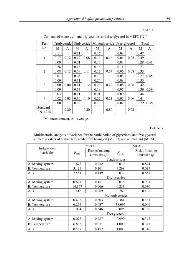
Agricultural biofuel production facilities 59
T a b l e 4
Contents of mono-, di- and triglycerides and free glycerol in MEFO [%]a
Test No.
Triglyceride Diglyceride Monoglyceride Free glycerol Total M A M A M A M A M A
1 0.11
0.120.11
0.080.16
0.16 0.09
0.05 0.47
0.41 0.17 0.12 0.16 0.04 0.490.09 0.01 0.15 0.03 0.28
2 0.28
0.120.18
0.110.16
0.14 0.11
0.08 0.73
0.45 0.08 0.09 0.12 0.06 0.350.01 0.05 0.13 0.08 0.27
3 0.00
0.000.11
0.120.24
0.22 0.08
0.08 0.35
0.39 0.00 0.11 0.23 0.08 0.420.00 0.13 0.19 0.07 0.39
4 0.03
0.020.11
0.100.21
0.21 0.09
0.06 0.44
0.38 0.02 0.10 0.22 0.07 0.410.00 0.08 0.19 0.02 0.29
Standard EN14214
0.20 0.20 0.80 0.02
aM –measurement, A – average.
T a b l e 5
Multifactorial analysis of variance for the participation of glycerides and free glycerol in methyl esters of higher fatty acids from frying oil (MEFO) and animal lard (MEAL)
Independent variables
MEFO MEAL
Fcalc. Risk of making a mistake (p) Fcalc.
Risk of making a mistake (p)
Triglycerides A. Mixing system 1.672 0.232 0.019 0.894 B. Temperature 3.425 0.101 7.268 0.027 A:B 2.551 0.149 0.037 0.851 Diglycerides A. Mixing system 0.627 0.451 0.016 0.903 B. Temperature 14.157 0.006 0.251 0.630 A:B 1.412 0.269 0.769 0.406 Monoglycerides A. Mixing system 0.492 0.503 2.381 0.161 B. Temperature 6.277 0.037 38.095 0.000 A:B 1.004 0.346 0.095 0.766 Free glycerol A. Mixing system 0.078 0.787 0.999 0.347 B. Temperature 6.832 0.031 1.000 0.347 A:B 0.558 0.477 1.003 0.346

W. GOLIMOWSKI, A. GRACZYK-PAWLAK 60
Based on the analysis of multifactorial variance, it has been established that only temperature influenced the content of glycerol particles. Neither the esterificator type nor factorial interactions between the two variables had any impact. Also, a correlation was observed between the dependent variables. The correlation for dependent va-riables has been calculated, including variable temperature, which had a major impact on the results. These results are shown in Table 6.
T a b l e 6
Correlation matrix of dependent variables and temperature
MEALMEFO Temperature Triglycerides Diglycerides Monoglycerides Free glycerol
Temperature –0.69 0.17 0.89 0.30 Triglycerides 0.47 0.45 –0.46 –0.24 Diglycerides 0.76 0.85 0.28 0.08 Monoglycerides 0.63 0.88 0.96 0.48 Free glycerol –0.66 0.07 –0.11 0.07
As a result of the statistical factorial analysis, it has been established that the participa-
tion of triglycerides in MEAL falls with the increasing temperature, whereas the participa-tion of monoglycerides increases. In the case of MEFO, there is a positive correlation be-tween temperature and the participation of glyceride particles as well as a strong positive intergroup correlation. This means that the higher the temperature, the higher the contents of glyceride particles. A negative correlation of free glycerol suggests that with the in-creasing temperature, the contents of free glycerol particles decreases.
4. CONCLUSION
Presence of unreacted fat particles in biodiesel obtained based on low-temperature esterification technology from waste fats is compliant with the European standard EN 14214 regarding biodiesel quality.
Increased content of free glycerol in all samples points at the necessity of imple-menting initial filtration of biodiesel in order to separate free glycerol particles.
As a result of a statistical analysis, a major impact of temperature on the content of the particles in question has been observed. A temperature increase results in de-creased reaction efficiency by increase of the content of glyceride particles in methyl esters from frying oil and decrease of the content of free glycerol. In the case of me-thyl esters from animal lard, a partly inversed correlation exists. Increasing tempera-ture of the reaction causes the concentrations of monoglycerides to increase and of triglycerides to decrease.

Agricultural biofuel production facilities 61
SYMBOLS
AL – animal lard FO – frying oil ME - methyl esters of higher fatty acids MEFO – methyl esters of higher fatty acids from frying oil MEAL – methyl esters of higher fatty acids from animal lard EH – hydraulically-mixing esterificator EM – mechanically-mixing esterificator
REFERENCES
[1] SZLACHTA Z., Power fuels from rapeseed of diesel engines, Wyd. Komunikacji i Łączności, War-szawa, 2002 (in Polish).
[2] BOCHEŃSKI C.I., Biodiesel agricultural fuel, Wyd. SGGW, Warszawa, 2003 (in Polish). [3] GRZYBEK A., Technologies transesterification of rapeseed oil, [In:] PODKÓWKA W. (Ed.), Biofuel
Glycerin Feed from rapeseed, Wyd. Uczelniane ATR, Bydgoszcz, 2004 (in Polish). [4] FRĄCKOWIAK P., J. Res. Replicat. Agricultural Eng., 2002, 47, 67. [5] ROSIAK E., Good economic situation for rape. Rape new challenges, Wyd. Biznes-Press, Warszawa,
2008 (in Polish). [6] WALISIEWICZ-NIEDBALSKA W., PODKÓWKA W., Fat acid methyl esters from cooking oil and animals,
[In:] PODKÓWKA W. (Ed.), Biofuel Glycerin Feed from rapeseed, Wyd. Uczelniane ATR, Byd-goszcz, 2004 (in Polish).
[7] SULEWSKI M., GACA J., BRZESKI S., Effect of oil quality and synthesis conditions on performance and selected parameters of biodiesel. II International Conference Energy Process Eco-Euro-Energy Bydgoszcz 2006, p. 365–373 (in Polish).
[8] WANG Y., OU S., LIU P., ZHANG Z., Energy Consvers. Manage., 2007, 48, 184. [9] LEUNG D.Y.C., GOU Y., Fuel Process Technol., 2007, 87, 883.
[10] PREDOJEVIĆ Z.J., Fuel, 2008, 87, 3522. [11] PHAN A.N., PHAN T.M., Fuel, 2008, 87, 3490. [12] GAWĘCKI J., Fats as ford components, [In:] GAWĘCKI J. (Ed.), The truth About Fats, Danone Insti-
tute, Warszawa, 1997, p. 1–2 (in Polish). [13] TASHTOUSH G.M., AL-WIDYAN M.I., AL-JARRAH M.M., Eng. Convers. Manage., 2004, 45, 2697. [14] WYATT V.T., HESS M.A., DUNN R.O., FOGLIA T.A., HAAS M.J., MARMER W.N., Jaocs., 2005, 82 (8),
585. [15] GOLIMOWSKI W., NOWAK A., Probl. Inż. Roln., 2008, 62 (4), 173. [16] ANGGRAINI A. A., LÖHRLEIN H. P., KRAUSE R., Possibilities and limits of the Re-Use cooking oils
with animals fat content as motor and heating fuel, [In:] Biomass for Energy and Industry, Proc. 10th European Conf. Technol. Exhib., Würzburg, Germany, June 1998, p. 572–574.
[17] SKOTT T., BioEnergy Research, 2007, 19, 6. [18] STRENZIOK R., WICKBOLDT P., Modification and optimization of a diesel engine for operation with
RME, [In:] Biomass for Energy and Industry, Proc. 10th European Conf. Technol. Exhib., Würzburg, Germany, June 1998, p. 634–638.
[19] GOLIMOWSKI W., NOWAK A., PAWLAK S., Biofuels from vegetables and animals fat, [In:] Selected Aspects of Current Environmental Conditions and Future Techniques in Animal Production, J.L. Ju-gowa (Ed.), IBMER, Warszawa, 2008 (in Polish).

W. GOLIMOWSKI, A. GRACZYK-PAWLAK 62
[20] PIKUL J., Characteristics and receiving animals fat, [In:] The Truth about Fats, J. Gawęcki (Ed.), Instytut Danone, Warszawa, 1997, p. 27–42 (in Polish).
[21] MATYSHOK H., KIEŻEL L.J., HOJNIAK M., Chemik, 1999, 52 (1), 6.
Environment Protection Engineering Vol. 37 2011 No. 4
BARBARA KUCHARCZYK*, WŁODZIMIERZ TYLUS*
EFFECT OF PROMOTOR TYPE AND REDUCER ADDITION ON THE ACTIVITY OF PALLADIUM CATALYSTS
IN OXIDATION OF METHANE IN MINE VENTILATION AIR
The aim of the study was to examine how the palladium precursors such as Pd(NO3)2 or PdCl2 and the reducers added (hydrazine hydrate or EDTA) influence methane combustion activity of monolithic palladium catalysts. Palladium nitrate was found to be a better Pd precursor, and the cata-lysts obtained displayed a noticeably higher activity in methane oxidation. The addition of hydrazine hydrate to 1% Pd/Al2O3 catalyst increased its activity when PdCl2 was used as the palladium precur-sor. With Pd(NO3)2 as the palladium precursor, the addition of reducers – hydrazine hydrate or EDTA – decreased the activity of the monolithic palladium catalysts tested.
1. INTRODUCTION
Palladium-based catalysts are characterized by a high methane combustion activ-ity which is influenced by the Pd precursor, the method of catalyst preparation and pretreatment, as well as the reaction conditions applied [1–7]. Pd precursors most fre-quently used are Pd(NO3)2, PdCl2 or H2PdCl4 [1–6], but use can also be made of palla-dium acetate, palladium propionate or other organic palladium salts dissolved in a variety of solvents [3, 4]. Catalysts obtained by dissolving those salts in carboxylic acids (acetic and propionic) exhibit very high activity [3]. The type of the precursor used influences the dispersion of Pd and the form in which it occurs on the surface of the Pd/Al2O3 catalyst [4]. When palladium acetate dissolved in toluene is used as a Pd precursor, the extent of Pd dispersion is higher than when use is made of Pd(NO3)2 or H2PdCl4. It was reported that Pd dispersion did not change after 24 h ageing of the Pd/Al2O3 catalyst at 650 °C [4]. Pd particles of the size smaller than 5 nm were
________________________ *Wrocław University of Technology, Institute of Inorganic Chemistry and Mineral Fertilizers,
Wybrzeże Wyspiańskiego 27, 50-370 Wrocław, Poland; corresponding author B. Kucharczyk, e-mail: [email protected]
B. KUCHARCZYK, W. TYLUS 64
quickly oxidized to PdO which alone was present on the catalyst surface. When Pd particles were of a larger size than 15 nm, palladium occurred in a metallic form and was covered with a PdO layer [4]. The form of Pd occurrence during methane oxida-tion – Pd0, PdO or PdOx/Pd – is ambiguous [1–4]. Depending on the reaction condi-tions (partial pressure of oxygen, temperature, composition of reaction mixture), PdO may undergo reduction or re-oxidation. The hydrocarbons present in the gas may in-duce the reduction of PdO at temperatures substantially lower than the temperature of its thermal decomposition in air or inert gas [6].
Methane emission is an inherent part of hard coal mining. As the emitted volume is large, methane has to be removed from the pit shaft with ventilation air for safety reasons. As methane concentration in ventilation air is low, not exceeding 0.75%, it cannot be fully utilized and in most instances methane is released into the atmosphere. The annual volume of methane entering the atmosphere with ventilation air ap-proaches 581million cubic meters [8]. Methane is a greenhouse gas [9] with an envi-ronmental impact 23 times as strong as that of carbon dioxide, and its presence in the atmosphere contributes to climatic changes and consequently to global warming.
Continual increase in the concentration of air-borne CH4 necessitates its removal from mine ventilation air. The best method for its removing in coal mines is catalytic combustion. Palladium catalysts on monolithic supports show a high activity in this process. The supports that may be used in catalytic combustion are either ceramic monoliths fabricated from aluminium oxide, silica, cordierite or mullite, or metallic monoliths made from heat-resisting foil of a 0.04–0.05 mm thick. Each of them has to be washcoated, e.g. with γ-Al2O3 of a high specific surface area. The washcoat is added to increase the specific surface area of the metallic support and stabilize its sur-face so as to prevent crystallite growth (at high temperatures, the crystallites of active components undergo sintering, causing them to increase in size) [10]. The benefits of applying monolithic supports are manifold: low cost of the support, possibility of us-ing a comparatively small amount of active layer, low flow resistance of gases at high flow velocities (>105 h–1), which enables application of high gas hourly space veloci-ties (GHSV) without considerable pressure drop on the catalytic layer [10]. As com-pared to ceramic monoliths, the walls of the support in metallic monoliths provide the catalyst with a larger free cross-section. As a result, the same conversion can be ob-tained at the volume of metallic monoliths which is by 20–30% lower than the volume of ceramic monoliths [10]. This is of importance when methane has to be removed from the ventilation air in coal mines because in that particular case large volumes of air are to be combusted, where methane concentration does not exceed 0.75%.
The aim of this work was to investigate the effect of Pd precursors and reducing agents chosen on the activity of the monolithic Pd catalyst in methane oxidation. The study included investigations into the specific surface area of the washcoat, Pd disper-sion and size of Pd crystallites, as well as XRD and SEM examinations of catalyst surfaces.

Activity of palladium catalysts in oxidation of methane 65
2. METHODS OF PREPARATION AND INVESTIGATION OF THE CATALYST
The supports for the catalysts were metal monoliths made of a 0.05 mm thick, Al2O3 washcoated heat-resisting FeCr20Al5 steel foil. They were shaped into cylinders with the height and diameter of 70 mm and 26 mm, respectively, possessing a honeycomb cross-section with 112 triangular channels/cm2 support. The washcoated support was calcined at 400 °C in air for 3 h. To obtain the active layer, 1% or 1.5% Pd (with the addition of 0.15% Al(OH)3 sol solution) was deposited onto the support by impregna-tion. Palladium nitrate with Pd concentration of 19.69% or palladium chloride with Pd concentration of 20.04% was used as the palladium precursor. The catalysts were cal-cined at 500 °C in air for 3 h. To increase Pd dispersion, additional catalysts were pre-pared, where the washcoated monolithic support was impregnated with the solutions of two reducing agents: hydrazine hydrate or ethylenediaminetetraacetic acid (EDTA). As for hydrazine hydrate, the washcoated support was subject to 12 h drying at 105 °C, followed by 10 min impregnation with hydrazine hydrate solution at 50 °C. EDTA was deposited by impregnation of the support with 0.1 M EDTA solution at 70 °C for 30 min, or for 5 min (Pd(NO3)2) and 12 min (PdCl2). Then the supports were subject to drying at 105 °C for 3 h, followed by deposition of 1.5% Pd from palladium nitrate or 1% Pd from palladium chloride. The catalysts are characterized in Table 1.
T a b l e 1
Preparation conditions, Pd dispersion, and average size of Pd crystallites
Catalyst Pd/Al2O3
[%]
Pd precursor
Reducer added
Impregnationtemperature
and time
Pd dispersion
[%]
Average size of Pd crystallites
[nm] 1.5 Pd(NO3)2 no reducer – 2.82 42 1.0 Pd(NO3)2 no reducer – 4.43 33 1.5 Pd(NO3)2 0.1M EDTA 70 °C, 5 min – – 1.5 Pd(NO3)2 0.1M EDTA 70 °C, 30 min 0.83 133 1.5 Pd(NO3)2 hydrazine hydrate 50 °C, 10 min 1.79 62 1.0 PdCl2 no reducer – – 61 1.0 PdCl2 0.1M EDTA 70 °C, 12 min – – 1.0 PdCl2 hydrazine hydrate 50 °C, 10 min – –
Methane combustion efficiency was tested using a laboratory flow reactor placed
in a heater with a programmed temperature increment (heating ramp 3 °C/min). Over the catalysts, 1% methane in air was oxidized at GHSV of 5800 h–1. Methane concen-tration in the gas mixture was measured with a Nanosens DP-27 analyzer.
BET surface area (SBET), average pore size and pore volume of the washcoat were determined by nitrogen sorption at the temperature of liquid nitrogen, using the ASAP 2010C apparatus (Micromeritics, USA). Active surface and dispersion of Pd were

B. KUCHARCZYK, W. TYLUS 66
determined with the same apparatus, based on measurements of hydrogen chemisorp-tion at 100 °C over the pressure range of 120–250 mm Hg.
XRD measurements were carried out using a PANalytical X’Pert Pro diffractome-ter with a Cu radiation source Kα of the wavelength of λ = 1.5418 Å. Use was made of the Bragg–Brentano scattering geometry. Morphology of the samples was examined by the scanning electron microscopy (SEM) with a Nova NanoSEM 230 microscope (made by FEI). Sample composition was determined by the energy dispersive X-ray spectrometry (EDXS), using an EDAX Pegasus XM4 spectrometer (with an SDD Apollo 40 detector) at 20 keV.
3. RESULTS AND DISCUSSION
Monolithic supports were covered with an Al2O3-based washcoat of the specific sur-face area (SBET) of 335.1 m2/g, total pore volume of 0.42 cm3/g, and pore diameter of 4.98 nm. Pd dispersion in the monolithic catalysts was poor (Table 1). In the case of the 1.5% Pd/Al2O3 catalyst, impregnation of the washcoated support with EDTA or hydra-zine hydrate solutions caused a decrease in Pd dispersion and consequently Pd crystallite growth. After 30 min of impregnation with EDTA, Pd dispersion dropped from 2.82% to 0.83%, and after 10 min of impregnation with hydrazine hydrate to 1.79%.
Impregnation of the support of the 1.5% Pd/Al2O3 catalyst with hydrazine hydrate solution at 50 °C for 10 min noticeably changed the appearance of the catalyst surface (Figs. 1 and 2). Although the surface of 1.5% Pd/Al2O3 with no reducer (Fig. 1) exhib-its cracks, no single crystallites are detected even at 10 000× magnification. This indi-cates the presence of very fine Pd crystallites.
Fig. 1. SEM image (left) and results of X-ray microanalysis (right) of the surface
of the 1.5% Pd/Al2O3 catalyst with no reducers; Pd precursor: Pd(NO3)2, magnification: 10 000×

Activity of palladium catalysts in oxidation of methane 67
After impregnation with hydrazine hydrate solution, the catalyst surface was covered with clusters of white crystallites. EDXS examinations have shown that Pd concentration in these crystallites is more than twice as high as in the grey fields on the catalyst surface (Fig. 2). White crystallites contain 6.05 at. % of Pd, 40.16 at. % of Al and 53.79 at. % of O, whereas in the dark fields of the surface 2.6 at. % of Pd, 45.9 at. % of Al and 51.5 at. % of O are found.
Fig. 2. SEM images and results of X-ray microanalyses of the surface of 1.5% Pd/Al2O3
catalyst impregnated with hydrazine hydrate solution at 50 °C for 10 min. Pd precursor: Pd(NO3)2
The XRD spectra of the 1.5% Pd/Al2O3 catalysts with no reducer addition and af-ter 5 min impregnation with EDTA solution (Pd precursor: Pd(NO3)2), as well as the XRD spectra of the 1% Pd/Al2O3 catalyst (Pd precursor: PdCl2), exhibit PdO peaks at 2Θ of 34° and peaks of heat-resisting FeCr20Al5 steel.
Fig. 3. Methane combustion activity of 1.5% Pd/Al2O3 catalysts with no reducer added, and after impregnation with EDTA and hydrazine hydrate

B. KUCHARCZYK, W. TYLUS 68
With Pd(NO3)2 as palladium precursor and in the absence of reducers, methane combustion efficiency increased when the Pd content increased from 1% to 1.5%. Over these catalysts, 100% conversion was achieved at 465 °C (1.5% of Pd) and 96% conversion at 509 °C (1% of Pd). Figure 3 shows temperature dependence of methane conversion over the 1.5% Pd/Al2O3 catalyst with Pd(NO3)2 as palladium precursor under the influence of EDTA or hydrazine hydrate addition. The activity of the cata-lyst was the highest when no reducing agent was added. Pd deposition onto the wash-coated support which was impregnated with 0.1 M EDTA solution for 5 min caused a substantial decrease in the catalyst activity despite the insignificant decrease in the size of PdO crystallites from 42 nm to 33 nm (XRD). Methane combustion efficiency decreased upon increasing the time of support impregnation. When the washcoated support was impregnated with hydrazine hydrate solution for 10 min, the decrease in the catalyst activity was lower than when EDTA solution was used.
Fig. 4. Methane combustion activity of 1% Pd/Al2O3 catalysts prepared
by various methods: 1 – Pd deposited without 0.15% Al(OH)3 sol, 2 – Pd deposited using Al(OH)3 sol; palladium precursor: PdCl2
When PdCl2 was used as palladium precursor, methane combustion efficiency in-creased with the Pd content of the catalyst from 1% to 1.5%. Figure 4 shows the effect of the preparation method used on the activity of the monolithic 1% Pd/Al2O3 catalyst. Palladium was deposited onto the surface of the washcoat prepared from Al2O3 pow-der in mixture with aluminium hydroxide sol (0.15% Al(OH)3) or without it. When use was made of the PdCl2 precursor, the 1% Pd/Al2O3 catalyst where Pd was depos-ited together with the 0.15% Al(OH)3 sol displayed a higher activity. In spite of this, its activity is noticeably lower as compared to the catalyst prepared with Pd(NO3)2 as the palladium precursor. This may be due to the poorer Pd dispersion and to the pres-

Activity of palladium catalysts in oxidation of methane 69
ence of larger Pd crystallites (Table 1) but also due to the poisoning effect of the chlo-rine persisting in the catalyst after calcination.
Fig. 5. Effect of the reducing agents (EDTA and hydrazine hydrate) on the methane combustion activity of the 1% Pd/Al2O3 catalyst;
palladium precursor: PdCl2, palladium deposited without Al(OH)3 sol
With PdCl2 as the palladium precursor and Pd deposition with no Al(OH)3 sol, im-pregnation of the washcoated support with hydrazine hydrate solution improves the activity of the catalyst (compared to the catalyst with no reducer added). When the same catalyst is impregnated with 0.1 M EDTA solution, its activity decreases mark-edly (Fig. 5).
4. CONCLUSIONS
The catalysts show a noticeably higher methane combustion activity with palladium nitrate than with palladium chloride as the Pd precursor. Regardless of the Pd precursor applied, their activity increases with the increase in Pd content from 1% to 1.5%.
The activity of the catalysts depends on the preparation method used. With PdCl2
as Pd precursor, the 1% Pd/Al2O3 catalyst where Pd was deposited together with the 1.5% Al(OH)3 sol exhibited a higher methane combustion activity.
The addition of solution of hydrazine hydrate improves the activity of the 1% Pd/Al2O3 catalyst when use is made of PdCl2 as the Pd precursor. With Pd(NO3)2 as the Pd precursor, methane combustion activity of the catalyst deteriorates.
The use of EDTA as a reducer decreases the activity of palladium-based catalysts irrespective of the Pd precursor applied.

B. KUCHARCZYK, W. TYLUS 70
ACKNOWLEDGEMENTS
The study was co-financed by the European Union from the European Regional Development Fund Project No. POIG.01.03.01-00-072/08 Program Innovative Econ-omy 2007–2013.
REFERENCES
[1] SCHLAM M., SOUZA M.M.V.M., ALEGRE V.V., PEREIRA DA SILVA M.A., CESAR D.V., PEREZ C.A.C., Catal. Today, 2006, 118 (3–4), 392.
[2] GELIN P., PRIMET M., Appl. Catal. B, 2002, 39 (1), 1. [3] KINNUNEN N.M., SUVANTO M., MORENO M.A., SAVIMAKI A., KINNUNEN T.J.J, PAKKANEN T.A.,
Appl. Catal. A, 2009, 370 (1–2), 78. [4] ROTH D., GELIN P., KADDOURI A., GARBOWSKI E., PRIMET M., TENA E., Catal. Today 2006, 112
(1–4), 134. [5] CIUPARU D., LYUBOVSKY M. R., ALTMAN E., PFEFFERIE L.D., DATYE A., Catal. Rev., 2002, 44 (4),
593. [6] RYOO M.W., CHUNG S.G., KIM J.H., SONG Y.S., SEO G., Catal. Today, 2003, 83 (1–4), 131. [7] MUSIALIK-PIOTROWSKA A., Ochr. Środ., 2011, 33 (1), 19. [8] Annual Report on Status of Basic Natural and technical Hazards in the Hard Coal Mining Industry,
GIG, Katowice 1986–2007 (in Polish). [9] KUJAWSKI O., Environ. Prot. Eng., 2009, 3, 27.
[10] NIJHUIS T.A., BEERS A.E.W., VERGUNST T., HOEK I., KAPTEIJN F., MOULIJN J.A., Catal. Rev. 2001, 43 (4), 345.
Environment Protection Engineering Vol. 37 2011 No. 4
ANDRZEJ BIELSKI*
MODELLING OF MASS TRANSPORT IN WATERCOURSES CONSIDERING MASS TRANSFER
BETWEEN PHASES IN UNSTEADY STATES. PART II. MASS TRANSPORT DURING ABSORPTION
AND ADSORPTION PROCESSES
Equations describing the rate of adsorption and absorption processes and those based on Whit-man’s model have been analyzed. In the case of unstable states, the mass flux penetrating to the layer of the river sediment and calculated by means of these equations differs from the mass flux calculated from the mass diffusion equation. In order to minimize the discrepancies between the flux determined by Whitman’s model and a real flux, the correction factor has been introduced into the concentration gradient equation originated from Whitman’s model. This correction factor can be expressed as a time dependence of the product of a certain parameter and the concentration derivative at the phase boundary (solid phase side). The corrected equation for the concentration gradient has been used to derive another equation, describing a general rate of the absorption and adsorption processes at the linear interfacial equilibrium and the chemical reactions occurring in the liquid and solid phases; the chemical reactions follow the first order monomolecular mechanism in unstable states with reference to the liquid phase. Knowing the general rate of the earlier mentioned processes it is possible to con-struct an advective-dispersion model of mass transport in a river including these particular processes. Such a model contains a term defined as a correction factor referring to the time dependence of the concentration derivative with respect to time. The described model may be also used for simulation of the transport of pollutants undergoing adsorption and absorption in the layer river sediment; the processes occur with a finite and infinitely large rate through the equilibrium states.
1. MASS TRANSPORT IN ABSORPTION AND ADSORPTION PROCESSES
Mass exchange between phases when there is no discontinuity of concentration at the phase boundary has been discussed in our previous paper [1]. In the case of ab-sorption and adsorption, concentrations associated with separate phases may take dif-
_________________________ *Cracow University of Technology, Department of Environmental Engineering, ul. Warszawska 24,
31-155 Cracow, Poland, e-mail: [email protected]

A. BIELSKI 72
ferent values next to the phase boundary. It is assumed that close to the phase bound-ary, the equilibrium between these concentrations is reached almost immediately [2]. In a general case, the relationships between these concentrations are described with nonlinear functions and only for sufficiently low concentrations it is possible to use a linear function (Henry’s law for the absorption equilibrium or for an adsorption iso-therm).
In the case of absorption or adsorption, the analysis of mass transport through a phase boundary may be carried out in a similar way as it was presented previously [1]. However, in such a case it would be necessary to solve the mass transport equa-tion in unsteady states (Eq, (1), [1])) for each phase separately to determine the con-centration distribution in a liquid phase and either in adsorption or absorption phases. Such approach to the analysis of mass transport through a phase boundary would re-sult in some major complications in calculations. Therefore, film Whitman’s model is used [2–5] to describe the mass transfer rate through a phase boundary.
Numerous other models of mass transfer exist, such as the Higbie penetration model, Danckwerst surface renewal model, Dobbins, Toor and Marchello model, Kisziniewski model, King model [2, 4]. Neither of them provides any possibilities to consider periodic or aperiodic concentration changes at the phase boundary though the models are little more complex than Whitman’s model. Just from the perspective of the mass transfer through a phase boundary in rivers, Whitman’s model seems to be the most appropriate.
For the specific case of absorption or adsorption without a chemical reaction, the model based on Whitman’s model may be described as follows:
( )*dc K c cdt h
= − − (1)
( )*
0
da K c cdt L
= − (2)
*a cΓ= (3)
Based on Fick’s law (Eq. (23), [1]) [4] and Eq. (1) it may be stated that:
( )*K D dcc ch h dy
⎛ ⎞− − = − −⎜ ⎟⎝ ⎠
(4)
After introducing Eq. (3) into Eq. (4) the concentration gradient is given by:
dc K acdy D Γ
⎛ ⎞= − −⎜ ⎟⎝ ⎠
(5)

Modelling of mass transport 73
Equation (5) refers to the average concentration gradient in the close vicinity of a phase boundary (Fig. 1).
Fig. 1. Distribution of concentrations inside liquid and solid phases. The dotted lines represent equilibrium concentrations
From Eqs. (2) and (3) it may be concluded that the degree of absorption or adsorp-tion may be described as:
( )00
0,t K aa a t x c d
Lτ
Γ⎛ ⎞= = + −⎜ ⎟⎝ ⎠∫ (6)
Using Equation (5), Eq. (6) may be transformed into:
( )0 0
0,tD dca a t x d
L dyτ= = − ∫ (7)
Substitution of Eq. (7) into Eq. (5) yields to expression for the concentration gradient:
( )0 0
0,tdc K K dc Kc d a t x
dy D L dy Dτ
Γ Γ= − − + =∫ (8)
In Equations (1)–(3) and the following, the equilibrium concentration was denoted as c*, the concentration at a phase boundary in a liquid phase was denoted as Ci while the concentration in a liquid phase core was denoted as c (Fig. 1). Equations (1) and (2) describe the mass transfer rate through a phase boundary. If concentration c was equivalent to Ci, the coefficient K would be defined as the penetration coefficient in a solid phase.
The first term of Eq. (8) refers to absorption or adsorption, while the second one to desorption processes. Let us use model (8) to analyze gradient changes for the concen-tration presented in Fig. 5 of [1].
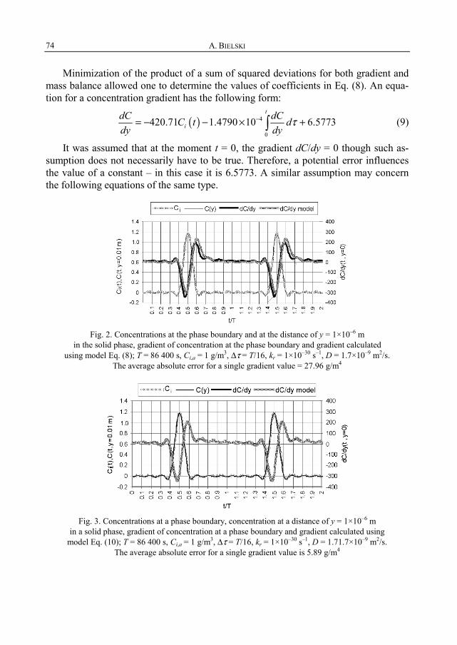
A. BIELSKI 74
Minimization of the product of a sum of squared deviations for both gradient and mass balance allowed one to determine the values of coefficients in Eq. (8). An equa-tion for a concentration gradient has the following form:
( ) 4
0
420.71 1.4790 10 6.5773t
idC dCC t ddy dy
τ−= − − × +∫ (9)
It was assumed that at the moment t = 0, the gradient dC/dy = 0 though such as-sumption does not necessarily have to be true. Therefore, a potential error influences the value of a constant – in this case it is 6.5773. A similar assumption may concern the following equations of the same type.
Fig. 2. Concentrations at the phase boundary and at the distance of y = 1×10⁻⁶ m in the solid phase, gradient of concentration at the phase boundary and gradient calculated
using model Eq. (8); T = 86 400 s, Ci,a = 1 g/m3, Δτ = T/16, kr = 1×10–30 s–1, D = 1.7×10⁻⁹ m2/s. The average absolute error for a single gradient value = 27.96 g/m4
Fig. 3. Concentrations at a phase boundary, concentration at a distance of y = 1×10⁻⁶ m
in a solid phase, gradient of concentration at a phase boundary and gradient calculated using model Eq. (10); T = 86 400 s, Ci,a = 1 g/m3, Δτ = T/16, kr = 1×10–30 s–1, D = 1.71.7×10–9 m2/s.
The average absolute error for a single gradient value is 5.89 g/m4

Modelling of mass transport 75
Model (8) shows substantial errors in calculations of the mass balance [6] (Fig. 3) and errors in calculations of the concentration gradient (Fig. 2) [6]. Its accuracy may still be improved by introducing a derivative of the concentration with respect to time, as it was proposed in previously (model (26) [1]). Then the model takes the form of:
( )1 2 3 40
ti
it
dC dC dCa C t a a d ady dt dy
τ= + + +∫ (10)
In the above equation, a constant a4 represents an initial value of absorption or ad-sorption – the value is zero in a particular case of an organic tracer introduced in an impulse mode. A term with the concentration gradient integral is responsible for de-sorption of the material back to a solid phase. The integral of a concentration gradient is proportional to the current value of absorption or adsorption. If the substance pre-sent in a solid phase is completely desorbed, the value of the integral is zero.
Minimization of the product of a sum of squared deviations for both gradient and mass balances allowed one to determine the values of the coefficients in Eq. (10) for the concentration curve presented in Fig. 5 of [1]. Now, the equation for the concen-tration gradient takes the following form:
( ) ( )
( )
4
5
0
( 224.30) 92.478 10
4.0725 10 15.209
ii
tt
dC dCC tdy dt
dC ddy
τ−
= − + − ×
+ − × +∫ (11)
Model (11) shows minor errors in calculation of the concentration gradient (Fig. 3) and a mass balance [6]. In Equation (11), the value of a4 different from zero is related to a periodic occurrence of impulses. Therefore, the average amount of ab-sorbed or adsorbed substance in a solid phase does not approach zero. It may be con-cluded that hardly any desorption process takes place, hence the concentration gradi-ent should take a positive sign and such situation occurs since a4 is positive.
Model (10) after its generalization may also be used as a tool for description of processes of absorption or adsorption accompanied with a chemical reaction in both liquid and solid phases.
If the reaction proceeds in solid phase with the rate (–kra), the concentration gra-dient has the following form:
( )0 0 0
0,t t
rr
dc K K dc K Kkc k d a t x c ddy D L dy D D
τ τΓ Γ
⎛ ⎞= − − + + = −⎜ ⎟
⎝ ⎠∫ ∫ (12)
In such a situation, the concentration gradient is expressed using the relationship similar to Eq. (10) including also the concentration integral in function of time (under a momentary assumption that: c ⇔ Ci)

A. BIELSKI 76
( )1 2 3 4 50 0
t ti
i it
dC dC dCa C t a a d a a C ddy dt dy
τ τ= + + + +∫ ∫ (13)
If the term including the concentration differential with respect to time is ignored in the above equation, the gradient and mass balance values are calculated with errors [6].
Based on Fick’s law (Eq. (23), [1]) [4] and the concentration gradient (Eq. (12)) rates r of absorption or adsorption accompanied with a chemical reaction with respect to a liquid phase may be calculated as:
( )
( )
*
* *
0 0 0
0 0 0
1
0,
0,
t tr
r
t tr
r
dm A dc D dcr Ddt V V dy h dy
K K D dc K Kkc k d a t x c dh L h dy h h
K K K Kkc k r d a t x c dh L h h
τ τΓ Γ
τ τΓ Γ
⎛ ⎞= − = − − =⎜ ⎟
⎝ ⎠⎛ ⎞
= − − + + = −⎜ ⎟⎝ ⎠⎛ ⎞
= − − + + = −⎜ ⎟⎝ ⎠
∫ ∫
∫ ∫
(14)
Since the overall process rate in the liquid phase is:
og cr r k c= − (15)
(rate of chemical reaction is (–krc)), based on Eq. (14), the following may be written:
( )0 0
0 0
0,t
og c r og
tr
c r
K K Kr k c k r d a t xh L h
Kk Kk k c dh L
τΓ Γ
τΓ
⎛ ⎞⎛ ⎞= − + − + + =⎜ ⎟⎜ ⎟⎝ ⎠ ⎝ ⎠⎡ ⎤⎛ ⎞
− + +⎢ ⎥⎜ ⎟⎢ ⎥⎝ ⎠⎣ ⎦
∫
∫ (16)
Considering a differential of concentration with respect to time in the equation for an overall process rate in a liquid phase, Eq. (16) takes the form:
1 2 3 4 50 0
t ti
og i og it
dCr a C a a r d a a C ddt
τ τ′ ′ ′ ′= + + + +∫ ∫ (17)
under the assumption that c ⇔ Ci. Parameter 2a′ = (D/h)a2 because after inserting the gradient equation, for example
Eq. (13) to Eq. (14), the parameter a2 will be multiplied through fraction (D/h). In the case of the concentration related to the core of a liquid phase, it may be
written that:
1 2 3 4 50 0
t t
og ogt
dcr a c a a r d a a c ddt
τ τ′ ′ ′ ′ ′= + + + +∫ ∫ (18)

Modelling of mass transport 77
Equation (18) describes a general process rate of absorption and adsorption at a linear interphase equilibrium accompanied with chemical reactions taking place in both solid and liquid phases; the reactions follow a monomolecular first order reaction mechanism, at an unsteady state with respect to a liquid phase. Parameters 1,a′ 4 ,a′ 5a′ and probably 2a′ (uncertainty origins from both analysis of a mass transport equation that includes absorption or adsorption processes carried on through an equilibrium states and Eq. (16)) depend on the water level h.
Coefficients 1 2 3 4 5, , , ,a a a a a′ ′ ′ ′ are characteristic of a certain type of wave. By changing wave parameters, e.g. the period T, number of harmonics, impulse duration, etc., parameters of Eq. (18) change as well.
2. POLLUTANT TRANSPORT MODEL
Advection-diffusion transport of any substance in natural water courses may be accompanied with chemical and/or physical processes such as absorption and adsorp-tion. The absorption and adsorption process rates are expressed as functions depending on concentrations of the analyzed substances within the phases participating in trans-port (e.g. liquid phase – water, solid phase related with water course sediment).
Substituting the overall rate (Eq. (18)) into a pollutant transport equation [7–14]:
1x og
c c cV E A rt x A x x
∂ ∂ ∂ ∂⎛ ⎞+ = ⋅ +⎜ ⎟∂ ∂ ∂ ∂⎝ ⎠ (19)
we arrive at an equation where the concentration derivative with respect to time is multiplied by a coefficient higher than 1 (1+ 2a′ ). Such a situation is similar to the one that occurs in the mass transport equation which takes into account processes of ad-sorption or absorption proceeding through the equilibrium states.
Using a classical approach of the mass transport model with other processes pro-ceeding with no equilibrium, the set of equations would be expressed as follows (case with a linear isotherm):
( )*1x c
c c c KV E A c c k ct x A x x h
∂ ∂ ∂ ∂⎛ ⎞+ = ⋅ − − −⎜ ⎟∂ ∂ ∂ ∂⎝ ⎠ (20)
( )*
0r
da K c c k adt L
= − − (21)
*a cΓ= (22)

A. BIELSKI 78
The set of equations does not have any additional term assigned to the concentration differential with respect to time, therefore calculations based on from Eqs. (20)–(22) would not give an accurate results.
Introduction of a new term at a differential ∂c/∂t in Eq. (20) leads to a model that consists of three equations:
( )*2
11 x cD c c c Ka V E A c c k ch t x A x x h
∂ ∂ ∂ ∂⎛ ⎞ ⎛ ⎞− + = ⋅ − − −⎜ ⎟ ⎜ ⎟∂ ∂ ∂ ∂⎝ ⎠ ⎝ ⎠ (23)
( )*2
0 0r
a K D cc c a k at L L t
∂ ∂= − − −∂ ∂
(24)
*a cΓ= (25)
Integrated with respect to time, Eq. (24) yields the dependence:
( ) ( ) ( )( ) ( )
( ) ( ) ( )
*
00
2 2 0 00 0
, , , ,
,
t
rKa x t c x c x k a x dL
D Da c x t a c x a xL L
τ τ τ τ⎛ ⎞= − −⎜ ⎟⎝ ⎠
− + +
∫ (26)
which may be easier to use in numerical applications. To solve the set of the above equations, the following conditions have to be for-
mulated: 1. Initial condition:
0( , 0) ( )C x t C x= = (27)
2. Boundary conditions related to: a) concentration changes in the initial cross-section:
( 0, ) ( )pC x t C t= = (28)
b) changes of the concentration gradient in the final cross-section (Neumann’s condition [15–19]:
odc ,
0x L t
Cx =
∂ =∂
(29)
(Lodc is the length of the water course segment) 3. Initial condition for adsorption or absorption:
( ) ( )0, 0a x t a x= = (30)

Modelling of mass transport 79
It should be noted, however that if a thermodynamic equilibrium exists between the phases at the initial moment, Eq. (25) or a similar one resulting from the actual isotherm has to be true. In particular, for a pure solid phase:
( ), 0 0a x t = = (31)
though, if an interfacial equilibrium exists, concentrations in a liquid phase are also zero, at the initial moment.
3. THEORETICAL ANALYSIS OF THE MASS TRANSPORT MODEL INCLUDING ABSORPTION OR ADSORPTION RATES
The mass transport model, including absorption and/or adsorption, comprises three equations: advection and diffusion in a liquid phase (Eq. (23)), absorption and/or adsorption rate (Eq. (24)) and interfacial equilibrium equation (Eq. (25), in this case Henry’s law). Equations (23) and (24) meet the conditions of the mass conservation law for the system [6].
If adsorption or absorption processes proceed through the equilibrium states, it may be shown that the model of mass transport fulfils the equations:
( )0 11 Lx d
L c c c qV AE r c ch t x A x x A
Γ ∂ ∂ ∂ ∂⎛ ⎞ ⎛ ⎞+ + = + + −⎜ ⎟ ⎜ ⎟∂ ∂ ∂ ∂⎝ ⎠ ⎝ ⎠ (32)
whereas the rate of changes of adsorption or absorption level is [6]:
0
a K a cct L t
Γ εΓ
∂ ∂⎛ ⎞= − +⎜ ⎟∂ ∂⎝ ⎠ (33)
Comparing Equations (33) and (24), as well as considering Eq. (25), the following relationship is obtained:
2 0Da LΓ ε− ⇔ (34)
A similarity of Eqs. (33) and (24) means that the set of Eqs. (23)–(25) may be used to simulate mass transport accompanied with adsorption/absorption processes proceeding at a finite rate through the equilibrium states. It may also be used in both cases simultaneously, when the sediment material consists of fractions that show dif-ferent physicochemical affinity to a substance transported in the water phase.

A. BIELSKI 80
4. IDENTIFICATION OF A MASS TRANSPORT MODEL ACCOMPANIED WITH ABSORPTION PROCESSES
The set of Eqs. (23)–(25) was used to describe propagation of copper sulfate in water. Water passed through a glass pipe partially filled with glass balls; the pipe length Lodc was ca. 0.70 m, its diameter d ca. 3 cm. In order to obtain very accurate results of measurements, the experiment was conducted in the laboratory. The pipe was slightly tilted up from its horizontal position and its upper end was equipped with an air release valve. This way the volume of a gas phase that built up over the water surface (air and water vapour) could be minimized. Water flowed over the entire cross-section of the pipe and only at the very end of the pipe both gas phase and free water level were present. Flow-through conductometric sensors were mounted at the both sides of the pipe to measure the conductivity in a real time. After calibration of sensors, it was possible to convert the measured conductivity into copper sulfate con-centration. Along the lower end of a pipe wall glass balls were placed; the ball diame-ter was 3 mm, thickness of a ball layer ca. 1.13 cm.
A polyethylene capillary was introduced inside the layer of glass balls and close to the air release valve, at the upper end of the pipe. The capillary enabled one to draw a sample from the inside of the glass ball layer. The layer of the glass balls together with water immobilized inside the layer was considered a solid phase with mostly absorption properties. Adsorption of copper ions on glass is very low if compared with their absorption in water that filled the space between glass balls. Therefore, it was absorption that was considered a leading process in a layer of balls. It was assumed that water motion in the interspace between balls is negligible if compared with the main stream motion over the glass ball layer and is therefore not considered in the transport of copper sulfate. During the experiment, water of high purity (specific con-ductivity of about 1 μS/cm) was used as a liquid phase. Conductivity of pure water was used as a reference value to calculate the copper sulfate concentration. Conduc-tivity measurements were performed including the temperature compensation coeffi-cient of 0.02 °C–1. Temperature of 25 °C was the reference temperature. All conductivity measurements were automatically converted to the values at the reference temperature. It was found that the relationship between specific conductivity S [μS/cm], and the concen-tration C [mol CuSO4·5H2O/m3] was as follows:
( )1.0566 3 6 0.657043.7361 10 5.4493 10C S S− −= × + × (35)
(Note: The values of the specific conductivity S in Eq. (35) are the readings of the conductometers for which the measuring constants were set in such a way as to make their readings identical. Hence, the results of Eq. (35) may slightly differ from the real values.)

Modelling of mass transport 81
4.1. EXPERIMENTAL RUNS
1 M copper sulfate solution was injected with a syringe to the water stream pass-ing through the pipe connected to the exit electrode. Characteristic of an input impulse is presented in Fig. 4. In practice, the volume of a copper sulfate solution injected to the water did not change the flow volume of Q = 3.48 cm3/s. The volume of the pipe V* that extended over the layer of glass balls was estimated as ca. 228 cm3. Based on this volume, the average hydraulic detention time in the system (tm = 228 cm3
/3.48 cm3/s = 65.59) as well as the average velocity V = 0.70 m/65.59 s = 1.067×10⁻² m/s were calculated. It should be noted that, the velocity calculated this way is lower than the real mass advection velocity; the difference may be attributed to the boundary layer present next to glass balls. Therefore, the actual volume V* of the liquid core was smaller than 228 cm3 and the estimated velocity V was just an approximation of the real advection velocity.
Fig. 4. Characteristic of the input impulse
Once the copper sulfate solution was introduced into the water stream, the conduc-tivity measurements were performed every 1 s and every 2 s, at the inlet and outlet of the system, respectively. Measurements were recorded automatically with a computer.
4.2. ESTIMATION OF MODEL PARAMETERS
In simulation calculations the model was used that comprised Eqs. (23)–(25). Ad-ditionally, a complementary variable ST6 and porosity of a balls layer ε0 were intro-duced to the model. Finally, the model could be written as:
( )*2 6
6 6
11 T x c
T T
D c c c Ka VS E A c c k ch ht x A x xS S
∂ ∂ ∂ ∂⎛ ⎞ ⎛ ⎞− + = ⋅ − − −⎜ ⎟⎜ ⎟ ∂ ∂ ∂ ∂⎝ ⎠⎜ ⎟⎜ ⎟⎝ ⎠
(36)

A. BIELSKI 82
( )*2
0 0 0 0r
a K D cc c a k at L L tε ε
∂ ∂= − − −∂ ∂
(37)
*a cΓ= (38)
The constant ST6 was introduced in order to compensate for the error caused by a rather rough determination of an advection velocity V. Since the velocity V increased along with a decrease of the water depth h, the term (h/ST6) in Eq. (36) appeared. Po-rosity ε0 of the layer of glass balls in Eq. (37) resulted from the assumption that copper salts were absorbed mostly by water that filled void spaces between balls. Therefore, based on the mass balance, thickness of the layer of glass ball L0 had to be multiplied by ε0.
The values of some model parameters were assumed for the calculations: h = 0.0109 m, V = 0.0107 m/s, A = 3.26×10⁻⁴ m2, kc = 0, ε0 = 0.409, L0 = 0.0113 m, kr = 0. The main goal of the experiment was to determine the values of the parameters or expressions: Ex, Da2, K, Γ and ST6, based on the experimental results.
The parameter values of model (Eqs. (36)–(38)) were identified using measurements of copper sulfate concentration in water passing through the installation. Additionally, the measurements of the concentration of copper sulfate in a layer of glass balls were consid-ered (absorption point in Table 1). The values of model parameters were determined by minimizing the sum of squared deviations between measured and calculated values. The function was minimized according to the simplex method of Nelder–Mead [20, 21].
T a b l e 1
Results of estimation of the model parametersa
Parameter or expression
One absorption
point
One absorption
point
Initial values No absorption
point
Two absorption
points
No absorption
point
No absorptionpoint v2
1 2 3 4 5 6 7 Ex [10–4 m2/s] 1.0236 0.61180 1.0829 5.2839 0.69805 0.42996 Da2 [10–3 m] –1.2966 − –0.64980 –7.9260 − − K [10–5 m/s] 8.6887 22.870 6.8685 23.236 10.849 22.873 Γ 1.0976 0.70157 1.0007 2.4553 0.68493 1.0156 ST6 1.3146 1.3874 1.2030 6.9646 1.2136 1.3676 Average absolute errormodel fitting [mol CuSO4·5H2O/m3]
0.002098 0.005491 0.004133 0.004407 0.006549 0.009507
aCoordinates of the experimental absorption point: t = 92 s, c = 2.430 mol CuSO4·5H2O/m3, coordinates of the theoretical absorption point t = 180 s, c = 1.637 mol CuSO4·5H2O/m3.
From the mathematical point of view, the model parameters may also be deter-mined if concentration measurements in a layer of glass balls are not considered (Ta-

Modelling of mass transport 83
ble 1, columns 4 and 5). In such a case, tough approximation of the model parameters may by ambiguous due to a multiminimum character of the sum of squared deviations between calculated and measured concentrations. The results presented in column 2 of Table 1 served as a basis for the essential plots that were later compared to the plots referring to the columns 3, 4 and 6.
Fig. 5. Concentration c and absorption a curves obtained from the model (Eqs. (36)–(38))
for data with absorption (Table 1, column 2) and without absorption ((–)abs) (Table 1, column 4)
Fig. 6. Concentration c and absorption a curves obtained from the model Eqs. (36)–(38) for data with absorption (Table 1, column 2) and without absorption ((–)abs v2) (Table 1, column 5)
Model parameters that have been determined based on the data both including and neglecting absorption level may assume similar or significantly different values (Ta-

A. BIELSKI 84
ble 1, columns: 2, 4 and 5). If the values are similar, the curves representing concen-tration c and absorption level a (Fig. 5) are also similar. Depending on the input values of model parameters, rather poor probability of the model parameters may be obtained after minimization of the sum of squared deviations (Table 1, column 5). A low value of the average absolute error of the model fitting, if compared with other errors, does not guarantee that the parameters values are accurate (Table 1, column 5). Curves of concentration c are in this case also similar, but the absorption level assumes irrational values (Fig. 6; concentrations in the absorption layer cannot exceed in this case con-centrations in the liquid phase). The value of the absorption coefficient Γ is close to 1.0 in this experiment (for the system water in a liquid phase – water in a solid phase of glass balls). The value of 2.4553 (Table 1, column 5) cannot refer to this phase sys-tem, although such a value is entirely correct just from the mathematical point of view. Questionable value of the coefficient Γ causes that the values of other parameters should also be considered as unlikely.
From the above discussion, it may be concluded that if the model (36)–(38) is to be used to analyze the quantity of substance in an absorption layer, it is necessary to obtain information on concentrations in this layer. Estimation of model parameters based on concentrations in just a mobile liquid phase may give wrong estimates. The results of actual measurements concerning liquid phase are usually used while model-ling processes of pollutant transport in rivers, lakes, sea etc. Such approach may result in poor estimation of model parameters. It should be stressed that transport of any substance in any medium (natural or man-mad, e.g. pipe, wastewater drain, chemical reactor) is always accompanied with absorption and/or adsorption processes – to less or more extend. Absorption processes may also be analyzed with respect to dead zones in units that carry the flow. Therefore, if the theoretical model has to describe accu-rately the course of the real-life processes, it is recommended to use the specific measuring data that enable one to determine the model parameter values. It should be noted that in the case of natural water bodies: rivers, lakes, sea etc., the values of Da2 and Γ are not known. Evaluation of the values of the parameters using other methods would not be much reliable. Therefore, they have to be estimated simultaneously with the values of other model parameters, and as such require the specific data.
Determination of concentrations in an absorption layer is difficult since measure-ments in this layer cause turmoil that interfere with the absorption process. In the ex-periment, in order to determine the concentration a, the sample volume of ca. 0.1 cm3 was taken from the layer core.
Assume that the product Da2 serves only as a correction factor for Whitman’s model to compensate for unsteady state conditions. Then, based on the estimated value –1.2966×10⁻³ m (Table 1, column 2), using equations published elsewhere (Eqs. (19), (22c) [1]) and assuming that the chemical process rate constant kr is 0 and the average wave period T ≈ 200 s, it is possible to determine the value of the effective coefficient of turbulent diffusion from a liquid to solid phase. In this case

Modelling of mass transport 85
D = Ez = 1.06×10⁻⁷ m2/s; the value is ca. 106 times higher than the molecular diffu-sion coefficient for copper sulfate.
Fig. 7. Concentration c and absorption a curves obtained from the model (Eqs. (36)–(38))
(Table 1, column 2) and model (Eqs. (36)–(38)) without term Da2 ((–)Da2) (Table 1, column 3)
Fig. 8. Concentration c and absorption a curves using model (Eqs. (36)–(38))
for the data including absorption (Table 1, column 2) and model (Eqs. (36)–(38)) without term Da2 ((-)Da2) for the data without absorption ((–)abs) (Table 1, column 6)
Neglecting the term Da2 in the model (Eqs. (36)–(38)) makes the model less ac-curate (the average absolute error of the model fit increases, Table 1, columns 3 and 6; Figs. 7 and 8). Absorption coefficients Γ are lower than the theoretical one, which is close to one. Also other values of the model parameters differ, specially the ab-
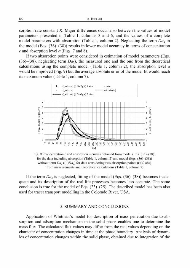
A. BIELSKI 86
sorption rate constant K. Major differences occur also between the values of model parameters presented in Table 1, columns 3 and 6, and the values of a complete model parameters with absorption (Table 1, column 2). Neglecting the term Da2 in the model (Eqs. (36)–(38)) results in lower model accuracy in terms of concentration c and absorption level a (Figs. 7 and 8).
If two absorption points were considered in estimation of model parameters (Eqs. (36)–(38), neglecting term Da2), the measured one and the one from the theoretical calculations using the complete model (Table 1, column 2), the absorption level a would be improved (Fig. 9) but the average absolute error of the model fit would reach its maximum value (Table 1, column 7).
Fig. 9. Concentration c and absorption a curves obtained from model (Eqs. (36)–(38))
for the data including absorption (Table 1, column 2) and model (Eqs. (36)–(38)) without term Da2 ((–)Da2) for data considering two absorption points ((+)2 abs)
from measurements and theoretical calculations (Table 1, column 7)
If the term Da2 is neglected, fitting of the model (Eqs. (36)–(38)) becomes inade-quate and its description of the real-life processes becomes less accurate. The same conclusion is true for the model of Eqs. (23)–(25). The described model has been also used for tracer transport modelling in the Colorado River, USA.
5. SUMMARY AND CONCLUSIONS
Application of Whitman’s model for description of mass penetration due to ab-sorption and adsorption mechanism in the solid phase enables one to determine the mass flux. The calculated flux values may differ from the real values depending on the character of concentration changes in time at the phase boundary. Analysis of dynam-ics of concentration changes within the solid phase, obtained due to integration of the

Modelling of mass transport 87
equation of diffusion in unsteady states, enables one to determine the real mass flux with respect to time. In order to decrease the discrepancies between the mass flux cal-culated from Whitman’s model and the real mass flux, it is necessary to introduce the correction factor to the equation describing the concentration gradient close to the phase boundary in a solid phase. The correction factor may be expressed as the prod-uct of a certain parameter and the concentration derivative with respect to time, at a phase boundary. The parameter is equivalent to the coefficient a2 (Eq. (22c), [1])) and therefore, it would be a function of: the concentration wave period, rate constant of chemical processes and the diffusion coefficient. The model comprises Eqs. (23)–(25) including the correction factor that incorporates the concentration de-rivative with respect to time. The model may be applied to simulate transport of pol-lutants which are subjected to adsorption or absorption processes in a river sediment layer. The processes proceed at a finite and an infinitely large rates through the equi-librium states. Therefore, the coefficient a2 stands for the correction factor improving accuracy of Whitman’s model and the parameter characterizing adsorption/absorption processes proceeding through the equilibrium states, simultaneously.
Model (23)–(25) was used to describe mass transport in a measuring apparatus; the experiments were conducted in a lab and in a full-scale model (river). The model accuracy improved when the term Da2 was different from zero. Knowing the value of this term, one can estimate the effective coefficient of turbulent diffusion in the direc-tion of the phase boundary, where the mass transport occurs.
SYMBOLS
(1/2)A0 – average concentration Ci, g/m3 A – surface area, m2 A* – surface normal to diffusion direction, m2 An, Bn – coefficients of a trigonometric series, g/m3 C, c – concentration, g/m3 C~ – concentration in a phase core, g/m3
~mC – average concentration within a phase core, g/m3 ~
,0mC – average concentration in a phase core at an initial river cross-section, g/m3 ~
,srdmC – average concentration in a phase core for a water course segment, g/m3 ~aC – concentration amplitude in a phase core, g/m3
C^ – Laplace transformation of a concentration function Ci – concentration at a phase boundary, g/m3 Ci,m – average concentration at a phase boundary, g/m3 Ci,a – concentration amplitude at a phase boundary, g/m3
iC∧ – Laplace transformation of a concentration at a phase boundary, g/m3 D – diffusion coefficient, m2/s Ex – longitudinal dispersion coefficient, m2/s Ez – coefficient of vertical turbulent diffusion (perpendicular to a solid phase surface), m2/s

A. BIELSKI 88
f – function G – transmittance g – acceleration of gravity h – water level or the average water level in a river, m i – drop of a water level in a water course, unless stated otherwise I – imaginary unit, kr – process rate constant, 1/s kw – coefficient of mass transfer at a liquid phase side, m/s; in the case of few different phases
indexes: 1, 2, etc. are used; units may differ depending on the formula kz,og – overall equivalent rate constant for all processes occurring in liquid and solid phases, s–1 L, L0 – thickness of a solid phase layer, m Lodc – length of water course segment, m M – transmittance module |G| m – mass, g r(C~) – process rate in the liquid phase core, g/(m3·s) rog – total process rate, g/(m3·s) Rh – hydraulic radius, m], re(...) – real part of complex variables im(...) – imaginary part of complex variables s – complex variable t – time, s t01, t02 – time of appearing and disappearing of a concentration impulse in a initial river cross-section, s tk1, tk2 – time of appearing and disappearing of a concentration impulse in a final river cross-section, s T – period of a function, s V – velocity, m/s Vsrd – average velocity, m/s V* – liquid phase volume, m3 x – linear coordinate (longitudinal for a river), m y – linear coordinate, m
GREEK SYMBOLS
αM, γM – complementary parameters Δt – time difference or time shift, s Δt1, Δt2 – time shifts, s Δt0, Δtk – time differences, s Δτ – impulse time, s ϕ – argument of transmittance G, rad ω – angular velocity, rad/s ω0 – angular velocity for the main harmonic, rad/s Ω1, Ω2 – integration constants
SELECTED SUBSCRIPTS
i – concentration at a phase boundary a – amplitude, unless the list of variables states otherwise m – average value, unless the list of variables states otherwise
SELECTED SUPERSCRIPTS
~ – phase core (in the case of concentration) ^ – Laplace transformation

Modelling of mass transport 89
REFERENCES
[1] BIELSKI A., Environ. Prot. Eng., 2011, 37 (2), 35. [2] KEMBŁOWSKI Z., MICHAŁOWSKI ST., STRUMIŁŁO C., ZARZYCKI R., Theoretical Basis of Chemical and
Process Engineering, WNT, Warsaw, 1985 (in Polish). [3] SZARAWARA J., SKRZYPEK J., Basis of Chemical Reactors Engineering, WNT, Warsaw, 1980
(in Polish). [4] POHORECKI R., WROŃSKI S., Kinetics and Thermodynamics of Chemical Engineering Processes,
WNT, Warsaw, 1977 (in Polish). [5] ZARZYCKI R., CHACUK A., STARZAK M., Absorption and Absorbers, WNT, Warsaw, 1987 (in Polish). [6] BIELSKI A., Selected Aspects of Mass Transfer Rate Determination between Phases in the Water-
course. Part III. Modification of Whitman’s Model for Concentration Changing in Time, Technical Bulletin, Cracow University of Technology, 2006, No. 2.
[7] BRUNNER G.W., HEC-RAS, River Analysis System, Hydraulic Reference Manual, Version 3.1, November 2002 (US Army Corps of Engineers, Hydraulic Engineering Center, http://www.hec.usace.army.mil
[8] BOWIE G.L., MILLS W.B., PORCELLA D.B., Rates, Constants and Kinetics Formulations in Surface Water Quality Modeling, Environmental Research Laboratory Office of Research and Development U.S. Environmental Protection Agency, Athens, Georgia, June 1985 (EPA/600/3-85/040), http://www.epa.gov//ordntrnt/ORD/WebPubs/surfaceH2O/surface.html
[9] FRANZ D.D, MELCHING C.S., Full Equations (FEQ) Model for the Solution of the Full, Dynamic Equations of Motion for One-Dimensional Unsteady Flow in Open Channels and through Control Structures, U.S. Geological Survey, Water-Resources Investigations Report, California, 1997, (http://water.usgs.gov/software/code/surface_water/feq/doc/feq.pdf).
[10] Ukrainian Center of Environmental and Water Projects, web page address: http://www.ucewp.kiev.ua, files address: http://www.ucewp.kiev.ua/publ/nazwa, name = { p1.pdf, p2.pdf, p3.pdf, …, p23.pdf }
[11] PUZYREWSKI R., SAWICKI J., Fluid Mechanic and Hydraulics, PWN, Warsaw, 1987 (in Polish). [12] LYNESS J.F., MYERS W.R.C., WARK J.B., J. Chart. Inst. Water Environ. Manage., 1997, 11 (5), 335. [13] HAIMES Y.Y., Hierarchical Analyses of Water Resources Systems, McGraw-Hill, New York, 1977. [14] CUNGE J.A., HOLLY F.M., VERWEY A., Practical Aspects of Computational River Hydraulics, Pitman
Publ. Ltd., London, 1980. [15] BIAŁAS S., OLAJOSSY A., Differential Methods of Solving Differential Equations. Part I, II, Technical
University of Mining and Metallurgy, Cracow, 1984. [16] SZYMKIEWICZ R., Mathematical Modelling of Flows in Rivers and Channels, PWN, Warsaw, 2000
(in Polish). [17] WESSELING P., Principles of Computational Fluid Dynamics, Springer, Berlin, 2001. [18] FLETCHER C.A.J., Computational Techniques for Fluid Dynamics, Vol. 1, 2, Springer, Berlin, 2000. [19] SAWICKI J.M., Pollutant Migration, Gdańsk Techn. Univ. Publ,, 2003 (in Polish). [20] SIENIUTYCZ S., Optimization in Process Engineering, WNT, Warsaw, 1978 (in Polish). [21] KRĘGLEWSKI T., ROGOWSKI T., RUSZCZYŃSKI A., SZYMANOWSKI J., Methods of Optimization in
FORTRAN, PWN, Warsaw, 1984 (in Polish).


Environment Protection Engineering Vol. 37 2011 No. 4
MOHAMED ALWAELI*
AN ECONOMIC ANALYSIS OF JOINED COSTS AND BENEFICIAL EFFECTS OF WASTE RECYCLING
Much research has been done throughout the world to determine the economic and ecological profitability of waste utilization as a substitution for raw materials. Unfortunately, Poland has no suf-ficient solutions in this field. The deficiency of solutions impedes the work of groups of specialists in various fields involved with the rational planning of recycling. This research seeks to offer a simple unified framework to study the key economic features of the use of waste as substitute for nonrenew-able resources in production in Poland and other countries. The purpose of this paper is to develop a model to obtain some key insights about the cost-effectiveness and define certain parameters which determine the effectiveness of production plants dedicated for processing waste into useful products. A plant’s productive possibilities can be described by the production function which is determined empirically. In this model, the emphasis is put on plant functioning and is dependent on the amount of work destined for the production in fixed units, technical maintenance costs of the work fixture in fixed units (e.g. machines’, cars’ operating costs etc.), and the amount of modified waste. In order to calculate these costs, we need to consider the issue of precise measuring the overhead costs in order to maximize profitability of this kind of measures allocation so that the profit will be the highest. The task of measuring overhead (costs) comes down to finding the maximum of the production function. This research presents the mathematical model and provides some key insights about the profitability of the plants dedicated for processing waste into secondary materials. In this research, we also deter-mined the maximum of the profit function and assess when the recycling plant will bring the profit and when it is the highest.
1. INTRODUCTION
We live in a socially interconnected world as well as in one displaying environ-mental interdependence. In most cases, human desires to use the Earth’s available resources, including environmental resources, exceed the capacity of these resources to satisfy human wants completely [1]. From an economic viewpoint, developing
_________________________ *Silesian University of Technology, Faculty of Energy and Environmental Engineering, ul. Konars-
kiego 18, 44-100 Gliwice, Poland, e-mail: [email protected]

M. ALWAELI 92
countries such as Poland are heavily dependent on living resources and natural envi-ronments. Furthermore, developed countries benefit substantially from the conserva-tion of their own resources through recycling/reuse.
The analysis of waste utilization as substitute natural resources has largely evolved as separate branches in economic literature. A notable exception is On Natu-ral Resources Substitution” by Andre and Creda, presenting a simple dynamic model to gain some key insights about the substitution of renewable resources for non-renewable resources, and the consequences for sustainability [2]. Ready and Ready presented a dynamic model according to which the price of landfill disposal increases from the time a new landfill is opened until it is filled, then decreases slightly as a new landfill is opened, and then begins increasing once again, due to the problem of land scarcity [3]. Therefore, it is economical to start recycling some of the waste before the price of landfill disposal reaches that of recycling, in order to reduce the costs of land-fill over time. In his pioneering work, Vivian [4] studied the costs and benefits of the current practice of dumping the construction waste into landfills and extracting new natural materials for new concrete production, as well as the proposed concrete recy-cling method to recycle the construction waste as aggregate for new concrete produc-tion. With the advent of the cost on the current practice, it is found that the concrete recycling method can result in huge savings.
The benefits gained from the concrete recycling method can balance the cost ex-pended for the current practice. Therefore, recycling concrete waste for new produc-tion is a cost-effective method that also helps to protect the environment as well as to achieve construction sustainability.
Towards the end of the 20th century, and at the beginning of the 21st century, the problem of using waste as a substitute for primary materials has become one of the basic issues of environmental protection and waste management in the world. Much research on recycling has been done by such authors as Rhyner [5], Sharma et al., [6], di Vita [7, 8], Fletcher and Mackay [9], Hsu and Kuo [10] Nakamura [11, 12], Ber-glund [13], Haque et al. [14] and Alwaeli [15, 16]. The authors analysed various mi-croeconomic models in which the economic profitability from waste recycling and certain ways of reducing the current value and future costs connected with waste man-agement were considered.
Over the last few decades, consumption behaviour in Poland has changed dramati-cally in accordance with rapid economic growth. Waste disposal caused serious prob-lems. Altogether more than 1.74 milliard tons of waste have been landfilled in Poland, and this amount increases approximately by 133 million tons every year [17]. Land-filling is still the main disposal method in Poland, although other methods are used on a negligible scale. Recycling is the most effective method for solving this problem because it not only reduces amount of waste, but also mitigates the depletion of natu-ral resources resulting from economic development.

An economic analysis of joined costs and beneficial effects of waste recycling 93
2. THE MODEL
The cost-effectiveness of waste recycling depends on a variety of inherent ex-penses. These costs include the expenses borne by the waste supplier, namely the cost of obtaining waste, transporting it to the segregation plants, and finally, the cost of the actual waste segregation. By contrast, recycling plants which use waste as raw materi-als bear the costs of waste processing as well as their clearance. In addition, we need to take into consideration those costs which are associated with amortization, equip-ment maintenance, waste storage, and labour. This work emphasizes the economic profitability of the plants dedicated for processing waste into secondary materials. The economic cost-effectiveness of the plant dedicated for processing waste into secondary materials can be defined as a production function. From economic experience [2, 7, 18] it seems that the production function has the form:
31 2 41 2 3 4 1 2 3 4( , , , )f x x x x ax x x xαα α α= (1)
In which coefficients a, α1, α2, α3, α4, are empirically matched and fulfil the following conditions:
2 3 4 1 2 3 40, 0, 0, 0, 1α α α α α α α α> > > > + + + <
The production function depends on the amount of work destined for the produc-tion in fixed units (x1), the technological maintenance costs of the work fixture in fixed units (x2), the amount of the modified raw material (x3), and the amortization costs (x4), etc.
Let us denote unit costs of particular elements of the production by q1, q2, q4, q4,. This means that the work unit costs q1 ZLP, technological maintenance unit of the work fixture costs q2 ZLP, etc. The unit of the product has the price of γ ZLP.
Having available x1, x2, x3, x4, the production plant will produce f(x1, x2, x3, x4) of the product units in a specific time unit (e.g. one month).
Owing to the fact that we have K means destined for the production in a given time, we get the condition that the sum of the input designated for the plant exploita-tion will not exceed K reduced by the permanent costs K1, (maintenance of both ad-ministration and plant). The aforementioned costs must be borne despite the volume of the production.
1 1 2 2 3 3 4 4 1q x q x q x q x K K+ + + ≤ − (2)
The left side of the inequality stands for the relative sum of the plant, whereas the right side signifies the amount of measures available.
We need to consider the issue of measuring overhead costs in order to ensure the highest possible profit. The profit from the production is expressed by the following formula:
M. ALWAELI 94
1 2 3 4 1 2 3 4 1 1 2 2 3 3 4 4( , , , ) ( , , , ) ( )x x x x f x x x x q x q x q x q xΦ γ= − + + + (3)
Because of the fact that the function increases with regard to each variable, the whole capital which we have at our disposal, must be divided. The following conclu-sion can be drawn:
1 2 3 4 1 2 3 4 10, 0, 0, 0,x x x x x x x x K K> > > > + + + = − (4)
The task of measuring overhead costs comes down to finding the maximum of the function (3) taking into account the aforementioned conditions (4). The mathematical solution to the issue of optimization will be discussed later.
Assuming that 1 2 3 4( , , , )x x x x is the solution to the problem, the profit from the plant operating in a specific time will be:
( ) ( )1 2 3 4 1 2 3 4 1, , , , , , ( )x x x x f x x x x K KΦ γ= − −
However, the profit must fulfil certain economic conditions. The value of the plant amounts to Π ZLP, the interest on the financial market in
a fixed time unit comes to p%, total depreciation of the working place amounts to q%. It may be concluded that the profit from the plant exploitation must be higher. Eventu-ally, it will come to:
1 2 3 4( , , , ) 0100 100
p qx x x xΦ Π− ⋅ ⋅ > (5)
The profit must be positive in order for the plant to have economic profitability. The profit issue of optimization will be solved based on the Kuhn–Tucker (K–T)
methods. From the K–T condition, if the system of equations
0, 1, 2, ...,i
L i nx
∂ = =∂
0Lλ
∂ =∂
has a positive solution
0, 1, 2, ..., , 0ix i n λ> = >
in which
( )1 1 2 2( , ) ( ) ... n nL x f x q x q x q x Kλ γ λ= − + + + −
is the Lagrange function, and the function for f(x) is a concave one which means that the solution of the system of Eqs. (5) is the solution to the problem of the maximiza-tion of the profit function

An economic analysis of joined costs and beneficial effects of waste recycling 95
( ) ( )x f x KΦ γ= −
Nevertheless, there is the condition
1 1 2 2 ... n nq x q x q x K+ + + =
Hence, we have the system of equations to be solved
0, 1, 2, ...,ii i
L f q i nx x
γ λ∂ ∂= − = =∂ ∂
1 1 2 2 ... 0n nL q x q x q x Kx
∂ = + + + − =∂
If the solution of this system is positive, it is a point in which the profit function reaches a maximum,
The profit function obtained from the production amounts to:
( ) ( )Z x f x Kγ= − (6)
where γ is the unit cost of the produced product, K – the amount of money destined for the production in a specific time (e.g. one month).
The function f(x) is the productive function depending on the means of production and is expressed as
1 21 2( ) ... n
nf x ax x xαα α= (7)
where:
1( ,..., ) nnx x x R+= ∈
10, 1, 2, ..., , 1
n
i ii
i n aα α=
> = = <∑
The function (7) is the concave one. We determine the maximum of the function Z(x) having the given condition
1 1 2 2 ... , 0, 1, 2, ...,n n iq x q x q x K x i n+ + + = > = (8)
in which (q1, q2, …, qn) is the vector of the unit prices of the means of production .nx R+∈
The Lagrange function
1 1 2 2( , ) ( ) ( ... ),n nL x f x q x q x q x K x Rλ γ λ += − + + + − ∈
and the Kuhn–Tucker function should be applied

M. ALWAELI 96
1 1 2 2
0, 1, 2, ...,
0
ii i
n n
L f q i nx xL q x q x q x K
γ λ
λ
∂ ∂⎧ ⎫= − = =⎪ ⎪∂ ∂⎪ ⎪⎨ ⎬
∂⎪ ⎪= + + ⋅⋅ ⋅+ − =⎪ ⎪∂⎩ ⎭
(9)
If the system has only one solution and ( , )L x λ is the concave function, the solu-tion is the maximum of the function given by Eq. (1). However, the condition in Eq. (3) must be fulfilled.
We determine the solution of the system depending on the parameter γ. Because of the fact that
1 11 ...( )... ( )i n i
i i ni i
f ax x x f xx x
α αα αα −∂ = =∂
the system of Eqs. (9) is represented by:
( ) 0, 1, 2, ...,ii
i
f x q i nxαγ λ− = =
For i j≠ we have
( )ii
i
f x qxαγ λ= (10a)
( )jj
j
f x qxα
γ λ= (10b)
Dividing Eq. (10a) by (10b), we obtain
, ,
i
i j ji i i i
j j ij j i j
ij j
x xx q q xq x q
qx q
αα
α α αα= = =
Hence, the vectors
( ) 1 21 2
1 2
, , ..., and , , ..., nn
n
x x x xq q q
αα α⎛ ⎞⎜ ⎟⎝ ⎠
have proportional coordinates; in consequence, we obtain
, 1, 2, ...,ii
i
x t i nqα
= =
where t is a parameter.

An economic analysis of joined costs and beneficial effects of waste recycling 97
After introducing the obtained values into Eq. (8) we get
1 21 2
1 2
... 0nn
n
q t q t q t Kq q q
αα α+ + + − =
The conclusion is that
1 2( ... )nt Kα α α+ + + =
Eventually,
Ktα
=
Consequently, we get the solution of the systems Eqs. (9) and (5)
· , 1, 2, ...,ii
i
Kx i nqα
α= =
which is the solution of the optimum task. The maximum profit, if we take into consideration investing K capital, amounts to:
1 2
1 2 1 2
1 21 2
1 2
... 1 2 1 2
1 2 1 2
( ) ( , ,..., ) ( ) ( ) ... ( )
( ) ( ) ( ) ...( ) ( ) ( , ,... )
n
n n
nn
n
n n
n n
K K KZ K Z x x x a Kq q q
K Ka K f Kq q q q q q
αα α
α α α αα α α
αα αγα α α
α αα α α αγ γα α
+ + +
= = ⋅ ⋅ ⋅ −
= − = −
Marking the constant
1 2
1 2
, , ..., ,n
n
f Rq q q
αα αγ ⎛ ⎞ =⎜ ⎟⎝ ⎠
we get
( ) KZ K R Kα
α⎛ ⎞= −⎜ ⎟⎝ ⎠
Now, we need to study how much money we have to invest in the production in order to achieve the maximuml profit. For this purpose, the variability of function
( )Z K must be studied
1( ) 1 0RZ K Kαα α
α−′ = − =
1 1R Kα αα − −=

M. ALWAELI 98
( )1/ 1K R αα −= ( ) ( ) ( ) ( ) ( )1/ 1 1/ 1 1/ 1 1/ 1 1/ 1( ) ( ) (1 )Z K R R R R R Rα α α α α αα α α− − − − −= − = − = −
Based on the fact that Z(K) = 0 for K = 0 and K = R1/(1–α)/α1/(1–α), the course of the function Z(K) is as shown in Fig. 1.
Fig. 1. Profit dependence on the invested capital
The unconditional extreme of the function (6), i.e. without the condition (8), is seen in the point
( )1/ 1 , 1, 2, ...,ii
i
x R i nq
α α−= =
For ( )1/ 1K R αα −> , it is uneconomic to invest K funds due to the fact that the profit from the production will be smaller than for the unconditional extreme.
3. DISCUSSION
It is a challenge to reduce the increasing flow of waste. The development of an ef-ficient waste recycling approach will help us to explore new opportunities for urban and environmental protection. Despite the fact that properties of the primary materials have been lost, the waste still carries both the value of subjective human work as well as the energy used for their production. This waste constitutes a potential source of secondary materials and fuels. Recycling is the most effective method for solving these problems because the recycling process not only reduces amount of waste, but also mitigates the depletion of natural resources resulting from economic develop-ment. Additionally, recycling reduces the cost of transportation and, relying on the analysis of the use of waste as a substitute in the production held by LCA, shortens, in some cases, the production process.

An economic analysis of joined costs and beneficial effects of waste recycling 99
Owing to the fact that we have K meaning destined for the production in a given time, we get the condition that the sum of the input designated for the plant exploita-tion will not exceed K reduced by the permanent costs K1, that is, the maintenance of both the administration and the plants.
Because of the fact that the production function increases with regard to each vari-able, the whole capital, which we have at our disposal, must be divided. We consi-dered the issue of measuring and dividing overhead costs, in order that the highest profit can be achieved.
The purpose of this research is to present the mathematical model and to provide some key insights about the profitability of the plants dedicated for processing waste into secondary materials. The profit function obtained from the production amounts to Z(x) = γ f(x) – K in which γ is the unit cost of the produced product, K is the quantity of money destined for the production in a specific time (e.g. one month) and f(x) is the production function.
In this research, we also determined the maximum of the profit function. Based on Eq. (6), the maximum profit, implicate that if we take into consideration investing K capital, amounts to:
1
( ) 1K RZ K R K KK
α ααα α
−⎛ ⎞⎛ ⎞ ⎛ ⎞= − = −⎜ ⎟⎜ ⎟ ⎜ ⎟⎜ ⎟⎝ ⎠ ⎝ ⎠⎝ ⎠
This means that the profit is proportional to the sum of invested capital K multi-
plied by the factor 1
1RK
ααα
−⎛ ⎞⎛ ⎞ −⎜ ⎟⎜ ⎟⎜ ⎟⎝ ⎠⎝ ⎠ which is decreasing upon increasing K. Thus in
order to have the maximum profit, we have to invest K = R1/(1–α)/α1/(1–α). Based on Fig. 1, the recycling plant will bring the profit for 0 < K < αR1/(1–α); nev-
ertheless, the profit is the highest for K = (αR2)1/(1–α. While for K > αR1/(1–α) it is un-
economic to invest K fund due to the fact that the profit from the production will be smaller than for the unconditional extreme.
Much research has been done throughout the world to determine the economic and ecological profitability of utilization of secondary materials (waste) as a substitution for raw materials. Unfortunately, Poland does not have sufficient solutions in this field. The deficiency of solutions impedes the work of groups of specialists in various fields involved with the rational planning of recycling. These are the results of our mathematical model of economic profitability of secondary materials (waste) utiliza-tion as the substitute for primary materials. Currently, no empirical analyses have been carried out on this issue. This research seeks to offer a simple unified framework to study the key economic features of the use of waste as substitute for nonrenewable resources in production in Poland and other countries.

M. ALWAELI 100
APPENDIX A
As a first attempt to evaluate the empirical performance of the model of the pre-vious section, we will consider example in which the production function is as fol-lows:
0,25 0,251 2 1 2( , )f x x x x=
The profit function amounts to 0,25 0,25
1 2 1 2 1 1 2 2( , )Z x x Px x q x q x= − −
where: P is the unit price of the produced product, q1, q2 – unit prices of raw materials. We need to determine the unconditional extreme of the function. We have
0,25 0,251 2
0,251 1 2 2 1 2 1 2 1
0.251 2
2 22 2
1 20,25 0,5 0,25 0,51 2 1 1 1 2 1 2 2 2 1 2
1 21 2
2
1 1 1 1 1 1 1, , ,4 4 4 4 4 4 2( )
2( )
1 1,2( ) 4 16 ( ) 2( ) 4 16 ( )
( , )4
( , )
fq q q q q q q q q q
PRq q
P P P Px xq q q q q q q q q q q q
Pf x xq q
PZ x y
α α ⎛ ⎞ ⎛ ⎞ ⎛ ⎞= = = =⎜ ⎟ ⎜ ⎟ ⎜ ⎟⎝ ⎠ ⎝ ⎠ ⎝ ⎠
=
⎛ ⎞ ⎛ ⎞= = = =⎜ ⎟ ⎜ ⎟⎝ ⎠ ⎝ ⎠
=
=2 2
1 2 1 2 1 24 8 8P P
q q q q q q− =
We can conclude that if we invest the means of production 1 2,x x , we will obtain the production 1 2( , )f x x whose profit amounts to ( , )Z x y .
APPENDIX B
Now we have to consider one more example in which the production function is as follows:
1 1 2 2( ) ln ln ... lnn nf x x x xα α α= + + +
where
1( ,..., ) , 0, 1,2, ...,nn ix x x R i nα+= ∈ > =
The function f(x) is concave for .nx R+∈
An economic analysis of joined costs and beneficial effects of waste recycling 101
The profit function
( ) ( )Z x Pf x K= −
where P is the price of the produced product, K the total sum of means destined for the production, i.e.
1 1 2 2 ... n nq x q x q x K+ + + =
where qi is the unit price of the used raw material. We maximize the Lagrange function
1 1 2 2( , ) ( ) ( ... )n nL x f x K q x q x q x Kλ γ λ= − − + + + −
We solve the system of equations
0, 1, 2, ...,ii
i i
L P q i nx x
α λ∂ = − = =∂
1 1 2 2 ... 0n nL q x q x q x Kx
∂ = + + + − =∂
we have
, 1, 2,...,ii
i
Pq i n
xα λ= =
For i j≠ we have
, jii j
i j
PP q qx x
αα λ λ= =
Dividing the equations by their members, we obtain
ji i
i j j
qx x q
αα=
Hence we get
j i
j i
ij
x x
qqα α= .
Therefore, the vectors
1 2( , ,..., )nx x x and 1 2
1 2
, ,..., n
n
xq q q
αα α⎛ ⎞⎜ ⎟⎝ ⎠
, are parallel.

M. ALWAELI 102
In that case there exists a constant such that
, 1, 2, ...,ii i
i
x t i nqα
= =
Substituting it into Eq. (8), we have
1 2 ... nt t t Kα α α+ + + =
Stating that
1 2 ... n aα α α+ + + =
we obtain
, Kta K ta
= =
consequently
, 1, 2, ...,ii
i
Kx i na q
α= =
is the solution to the problem of maximization. We have
1 21 2
1 2
1 21 2 1 2
1 2
( ) ln ln ... ln
( ... ) ln ln ... ln ln ( )
nn
n
nn n
n
K K Kf xa q a q a q
K Ka f xa q q q a
αα αα α α
αα αα α α α α α
= + + +
= + + + + + + + = +
Therefore the maximum profit from the production process is
( ) ( ln ( ))KZ x P a f x Ka
= + −
Stating that ( )Pf x R= we have
( ) ln KZ x Pa K Ra
= − −
We investigate which means have to be involved so that the profit is maximized. We have
( ) 1 0dZ x PadK K
= − =
thus K = Pa.

An economic analysis of joined costs and beneficial effects of waste recycling 103
Therefore, the maximum profit amounts to
ln for , 1, 2, ..., ii
i
PZ Pa P Pa R x i nqα
= − − = =
REFERENCES
[1] TISDELL C.A., Economics of Environmental Conservation, 2nd Ed., Edward Elgar, Cheltenam., UK, 2005.
[2] ANDRE F.J., CREDA E., Resour. Policy, 2006, 30 (4), 233. [3] READY M., READY R., J. Environ. Econ. Manage., 1995, 28 (3), 307. [4] VIVIAN W.Y.T., Resour. Conserv. Recycl., 2008, 52 (2), 821. [5] RHYNER CH.R., Resour. Conserv. Recycl., 1998, 24 (3-4), 349. [6] SHARMA V.K., BEUKERING V.P., BARNALI N., Resour. Conserv. Recycl., 1997, 21 (1), 55. [7] DI VITA G., Resour. Policy, 2006, 31 (3), 172. [8] DI VITA G., Ecol. Econ., 2007, 63 (1), 138. [9] FLETCHER B.L., MACKAY M.E., Resour. Conserv. Recycl., 1996, 17 (2), 141.
[10] HSU E., KUO C.M., Waste Manage., 2005, 25 (1), 53. [11] NAKAMURA S., Ecol. Econom., 1999, 28 (1), 1333. [12] NAKAMURA S., KONDO Y., Ecol. Econom., 2006, 57 (3), 494. [13] BERGLUND C., Ecol. Econom., 2006, 56 (4), 560. [14] HAQUE A., MUJTABA I.M., BELL J.N.B., Waste Manage., 2000, 20 (8), 625. [15] ALWAELI M., Mineral Energy Economy, 2008, 24 (4/1), 19. [16] ALWAELI M., Environ. Prot. Eng., 2011, 1, 51. [17] Statistical Yearbook, GUS, Poland, 2008. [18] SHARMA V.K., BEUKERING P.V., NAG B., Resour. Conserv. Recycl., 2007, 21 (1), 57.


Environment Protection Engineering Vol. 37 2011 No. 4
ANDRZEJ KOTOWSKI*, HENRYK SZEWCZYK**, WOJCIECH CIEŻAK*
ENTRANCE LOSS COEFFICIENTS IN PIPE HYDRAULIC SYSTEMS
The entrance loss coefficients have been investigated for four, most frequently occurring geo-metric shapes of inlets placed on the reservoir bottom. The minor (entrance, inlet) losses coefficients determined in the paper, having not been investigated experimentally so far, may be used, for exam-ple, to correctly dimension throttling pipes. Throttling pipelines are commonly used in sewage sys-tems for limiting the volume flow rate of sewage channelled to sewage treatment plants from storage reservoirs, storm overflows or rainwater separators during torrential rainfall.
1. INTRODUCTION
The possibility to find correct values of entrance resistance coefficients of pipes in hydraulic systems given in available manuals, handbooks or standards and similar materials is only illusory. This is no surprise, since the coefficients are determined by specific shapes of a given minor loss and, in general, depend on the Reynolds number (Re). However, in practice, the Reynolds number is so high that the K coefficient can be constant. The paper presents the results of investigation of four specific shapes of pipe inlets typical of hydraulic (particularly sewage) systems, which however, have not been hydraulically investigated so far.
The sewage flow from a number of sewage facilities (storage reservoirs, storm overflows, separators) occurring during torrential rainfall must be limited prior to its introduction to the sewage treatment plant. To this end various types of flow regula-tors are used. However, most often this is realized by means of a pipeline working under pressure called a throttling pipe [1, 2]. The throttling pipe is an example of liq-uid flow regulator which makes it possible to empty a reservoir completely because it _________________________
*Institute of Environmental Protection Engineering, Wrocław University of Technology, pl. Grun-waldzki 9, 50-370 Wrocław, Poland, e-mail addresses: [email protected] (corresponding author), [email protected]
**Institute of Thermal Engineering and Fluid Mechanics, Wrocław University of Technology, Wybrzeże Wyspiańskiego 27, 50-370 Wrocław, Poland, e-mail: [email protected]

A. KOTOWSKI et al. 106
is placed on its bottom level. Minor losses on the inlet and outlet of a throttling pipe – apart from linear losses – influence the selection of the length and diameter of the pipe which should ensure the assumed distribution of volume flow rates on a storm overflow [3–5], or in a light liquid separator with inner by-pass channels [6].
The calculation of dimensions (diameter and length) of a throttling pipe is based on the phenomenon of liquid flow between two open reservoirs and connected by means of a pipeline operating under elevated pressure. Its correct dimensioning re-quires the knowledge of the linear ( f ) and minor (K) loss coefficients because they appear in the Darcy–Weisbach formula which is used to calculate energy losses in closed conduits. Therefore, the energy loss head Dhl,d occurring in liquid flow with the mean velocity u through the pipeline of the diameter d and length l amounts to
2
,Δ2l d
l uh f Kd g
α⎛ ⎞= + +⎜ ⎟⎝ ⎠
(1)
These are the entrance resistance of the coefficient K and outlet resistance of the coefficient α. It should be noted that the entire kinetic energy is lost on the outlet of the throttling pipe [6], thus, the outlet loss head is αu2/2g (α is the kinetic energy cor-rection factor).
As can be seen from Eq. (1), the knowledge of correct values of coefficients f, K and α is essential in the procedure of dimensioning of the throttling pipe. Thus, the friction factor f, which depends on relative roughness k/d (where k is a mean wall roughness head) and the Reynolds number and hence f = f (k/d, Re), is assumed ac-cording to known formulae or from nomograms [8]. In the case of plastic sewage pipes of the wall smoothness comparable to glass the friction factor can be then calcu-lated from the Blasius formula [7–11]:
4
40.3164π
Vqudf RedRe ν ν
= ∧ = = (2)
where: ν is the kinematic viscosity (it was calculated using the formula making it de-pendent on the water temperature) and qV is volume rate of flow.
As already mentioned, the entire kinetic energy is lost on the outlet of the throt-tling pipe, therefore the outlet loss head is αu2/2g. However, in many textbooks and publications [7, 10, 12] the outlet loss coefficient (α) is assumed equal to 1. It is nearly consistent with reality but only for a high turbulent flow. Whereas, Szewczyk [13] gave the following explicit dependence for the kinetic energy correction factor valid in the wide range of Re ∈ [2.8×10³, 36×106[, for the flow in smooth hydraulic pipes
6 4 210 10 101 0.101 0.107 0.113ln ln lnRe Re Re
α ⎛ ⎞ ⎛ ⎞ ⎛ ⎞= + − +⎜ ⎟ ⎜ ⎟ ⎜ ⎟⎝ ⎠ ⎝ ⎠ ⎝ ⎠
(3)

Entrance loss coefficients in pipe hydraulic systems 107
In order to illustrate the course of the dependence α(Re), a number of values of α calculated from Eq. (3) were given, that is: α({5, 10, 102, 103}μ103) = {1.22, 1.15, 1.07, 1.04}.
The selection of values for the inlet loss coefficient K encounters a number of dif-ficulties, since literature data differ by as much as 100%. Typically, the Borda–Carnot formula was employed here [7, 10, 14, 15] and for the outflow from a large reservoir to the throttling pipe K is obtained as equal 0.5. According to the model testing on lateral overfalls with throttled outflow carried out by Kallwass [16, 17], values of the outlet loss coefficient amount to: K = 0.25, for the round-edged inlet, or K = 0.35 for the sharp-edged inlet. However, Imhoff and Imhoff [18] and the TGL standard [19] recommend to assume K = 0.40, if edges are technically sharp, but according to the DVWK-ATV-A 111 guidelines [1] give K = 0.45.
The reservoir wall containing the throttling pipe can be flat and perpendicular to the pipe axis, but it may also contain bevels – guides (usually at the angle of π/4 rad), and finally, the reservoir bottom may contain invert channels (typically of the depth of d/2). Furthermore, the influence of the height and width of a liquid jet in front of a pipe inlet have not been investigated.
2. THE IDEA OF ENTRANCE LOSSES MEASUREMENT, INVESTIGATION PROGRAM AND TESTING STATION
Figure 1 shows an idealized, axially symmetrical case of laminar and turbulent liquid flows through a straight pipe of the length more than le and diameter d connect-ing two quasi infinite liquid areas (areas of recirculation behind the pipe inlet were omitted for simplification).
The average flow velocity in the pipe amounts to u, whereas the shape of velocity distribution is formed at the entrance length le obtaining an unchangeable shape, char-acteristic of laminar or turbulent flow, only behind this length. Therefore, on the length le the energy grade line (EGL) drop is descending to become steady behind the entrance length. As can be seen, the minor loss is spread on the entire entrance length le, which in laminar flow amounts to approximately 0.06Red and le ≈ 40d* in a turbu-lent flow. For practical reasons, energetic losses in the conduit are shown in the form of a simple sum of two components: minor losses and friction losses changing real curves EGL and HGL (the hydraulic grade line) into their apparent courses, which were marked with dotted lines in Fig. 1. As it can be seen in the figure, K cannot be well determined based on differential pressure p0 – pi measurements in front of the inlet and in the section ]0, le[, especially, when the value of K being measured is as _________________________
*Some authors give different values, e.g. according to Schlichting [20] le ∈ [25, 40]d (in a turbulent flow).

A. KOTOWSKI et al. 108
small as in the investigated case. A method similar to the one, forced by many authors, can be used to determinethe minor losses coefficient of fittings offering a high resis-tance, e.g. a flow regulating valve. Then, two measurement sections are located close in front of and behind a fitting being investigated and their velocity heads are assumed identical, whereas friction losses are typically omitted. Such assumptions are not ac-ceptable in the investigated case, where K is ca. 0.5 and f is ca. 0.02, and if the meas-urement is performed in a typical distance of 5d behind the inlet*, then friction losses constitute 0.2 of minor losses. It should be emphasized that the subject of the investi-gations was a flow far more complex than the one shown in Fig. 1. Namely, there is no axial symmetry of flow and recirculation areas are present, which were not accounted for in the figure.
Fig. 1. Laminar (a) and turbulent (b) flows in the entrance of the tube, EGL – the energy grad line, VH – the velocity head, HGL – the hydraulic grade line,
BL – the boundary layer, α – the kinetic energy correction factor (αe≈1), le – the entrance length, pk (k ∈ {i = 1, 2; 0, e}) – the liquid pressure
_________________________ * Notice that additionally the measurement section may be located beyond a recirculation zone and in
the section ]0, le[ the kinetic energy correction factor a is unknown [21].

Entrance loss coefficients in pipe hydraulic systems 109
A similar explanation of the shape of the phenomenon velocity of distribution for-mation and interpretation of inlet losses are given by White [10] and Szewczyk [13].
The investigations aimed at determining the influence of geometrical shapes most frequently used in engineering practice forming reservoir sections adhering to the inlet of the pipe on its inlet resistance. The investigations covered:
• measurements related to the identification and calibration of model elements, which include: the inner diameter of polypropylene pipes used to produce the throt-tling pipe, the hydraulic characteristic of a triangular measuring overfall and physico-chemical properties of circulating water used for the investigations,
• measurements related to the implementation of the fundamental paper objective, that is: determination of the piezometric pressure heads in hydrometric sections, measurements of water volume flow rates (by means of the overfall) for varying depths of reservoir filling and for different shapes of its inlet section adhering to the throttling pipe and variable heights (z0) and widths (b) of the water jets, and finally, measurements of water temperature.
The inner diameter of polypropylene pipeline being investigated was determined by measuring the volume of water filling a pipe section of the known length, obtaining d = (71.0±0.1) mm. The hydraulic characteristic of the triangular measuring overfall (of the angle of π/2 rad) were determined by the volumetric method, establishing its flow coefficient at m = 0.600. The physicochemical properties of water used in the investigations were verified at the beginning, in the middle and at the end of investiga-tions, while the composition of circulating water during the test proved to be stable.
Fig. 2. The shapes of pipe inlets (1–4): vertical cross-sections and horizontal projections (b/d ∈ {1.25, 2.5, 5, 10}, h/d ∈ {2.5, 5, 10, 19})
The testing program covered four basic options of geometrical shapes of reser-voirs in the section adhering to pipe inlets that is (Fig. 2):
1) a flat wall perpendicular to the throttling pipe axis with sharp-edged inlet, with-out an invert channel on the reservoir bottom;
1 2 3 4
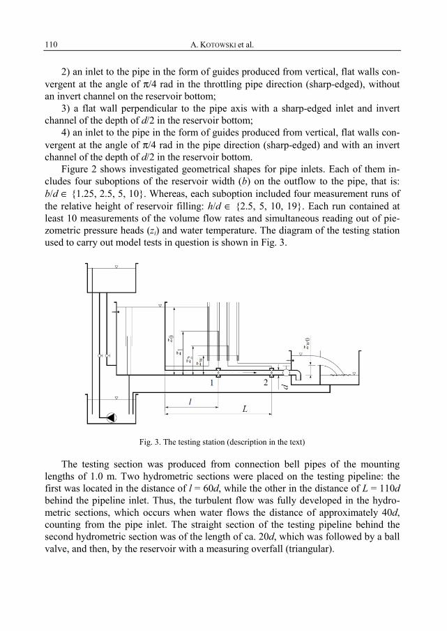
A. KOTOWSKI et al. 110
2) an inlet to the pipe in the form of guides produced from vertical, flat walls con-vergent at the angle of π/4 rad in the throttling pipe direction (sharp-edged), without an invert channel on the reservoir bottom;
3) a flat wall perpendicular to the pipe axis with a sharp-edged inlet and invert channel of the depth of d/2 in the reservoir bottom;
4) an inlet to the pipe in the form of guides produced from vertical, flat walls con-vergent at the angle of π/4 rad in the pipe direction (sharp-edged) and with an invert channel of the depth of d/2 in the reservoir bottom.
Figure 2 shows investigated geometrical shapes for pipe inlets. Each of them in-cludes four suboptions of the reservoir width (b) on the outflow to the pipe, that is: b/d ∈ {1.25, 2.5, 5, 10}. Whereas, each suboption included four measurement runs of the relative height of reservoir filling: h/d ∈ {2.5, 5, 10, 19}. Each run contained at least 10 measurements of the volume flow rates and simultaneous reading out of pie-zometric pressure heads (zi) and water temperature. The diagram of the testing station used to carry out model tests in question is shown in Fig. 3.
Fig. 3. The testing station (description in the text)
The testing section was produced from connection bell pipes of the mounting lengths of 1.0 m. Two hydrometric sections were placed on the testing pipeline: the first was located in the distance of l = 60d, while the other in the distance of L = 110d behind the pipeline inlet. Thus, the turbulent flow was fully developed in the hydro-metric sections, which occurs when water flows the distance of approximately 40d, counting from the pipe inlet. The straight section of the testing pipeline behind the second hydrometric section was of the length of ca. 20d, which was followed by a ball valve, and then, by the reservoir with a measuring overfall (triangular).

Entrance loss coefficients in pipe hydraulic systems 111
The adjustment of the valve, as well as of other valves shown in Fig. 3, made it possible to set required parameters (h/d, qV). The remaining values of quantities neces-sary to determine the loss coefficients (f, K) and Reynolds number (Re) were read out from piezometers (zi, i ∈ {0, 1, 2, w}), and water temperature was measured in two locations shown in Fig. 3. Water was supplied to the piezometers by means of circuit pressure delivery chambers to which pressure signal was provided through 4 piezo-metric holes («3 mm), drilled precisely and symmetrically in the pipe circumference. The obtained volume flow rates were in the range ]1.45, 10.3[ dm3/s, while the water flow velocities were in the range ]0.37, 2.6[ m/s, the temperatures of water were in the range ]7.0, 13.1[ °C thus, the flow was always turbulent, since Re ∈ ]19, 155[μ103.
3. RESULTS OF INVESTIGATIONS
3.1. THE OUTPUT EQUATIONS FOR FRICTION FACTOR AND MINOR LOSS COEFFICIENT
By writing generalized Bernoulli’s equation in relation to the comparative level located on the inlet chamber bottom, set for the first section lying on the water surface in the chamber and for the second cross-section of the water jet flowing through the pipe, the following two equations can be yielded in the form of
2 2 2
0 2 2 2
4 4 41 1 1 ,π 2 π 2 π 2
{ , } {{1, },{2, }}
V V Vi
q q qz z f Kd g d d g d g
i l L
Λα
Λ
⎛ ⎞ ⎛ ⎞ ⎛ ⎞= + + +⎜ ⎟ ⎜ ⎟ ⎜ ⎟⎝ ⎠ ⎝ ⎠ ⎝ ⎠
∈
(4)
which gives the following dependences with regards to f and K
2 5 1 2
2
π
8 V
z zgdL l L lf
q
⎛ ⎞−⎜ ⎟− −⎝ ⎠= (5)
2 4 1 20
2
π1 1
8 V
z zgd z l LL lK
qα
⎛ ⎞− +⎜ ⎟− −⎜ ⎟
⎝ ⎠= − (6)
The fact that the flow in Sections 1 and 2 is fully developed was accounted for, thus α is identical there. It follows from Eqs. (5) and (6) that owing to the applied compensatory measurement method the influence of the minor losses on the measured value of the friction factor and the influence of the friction losses on the measured value of the minor loss coefficient can be eliminated. It can be seen from Eq. (6) that

A. KOTOWSKI et al. 112
a sufficiently accurate knowledge of the kinetic energy correction factor is very impor-tant in the measurement procedure of the coefficient K. It should be remembered that the minor loss coefficient has the numerical value of the order of 0.5 in relation to α > 1.04, and thus, the assumption of α = 1 involves the error of the order of 10% measurement results of the factor K.
In the experiment, it can be acknowledged that the pipe is hydraulically smooth, because the empirically obtained dependence of f (Re) diverges insignificantly from the Blasius curve (2). This is illustrated in Fig. 4, which shows the results of the de-termination of the friction factor f based on thet measurements using Eq. (5). The vol-ume flow rate qV, as in Eqs. (5) and (6), was determined based on equation specifying the liquid flow through the measuring triangular overfall (Fig. 3)
50
8 2 ( )15V w wq g z zμ= − (7)
In Equation (7), m = 0.60 was taken as the value obtained as a result of the overfall calibration on the testing station presented in the Fig. 3.
Fig. 4. The dependence f (Re) obtained empirically by the authors (the solid line is the Blasius curve)
In Figure 4, the results of all measurements (the total of 719) are given. They are marked with circles, therewith, the grey circles indicate results recognized as inaccu-rate – divergent by more than 5% from the mean value (there were 18). The square centers visible in Fig. 4 contain coordinates of mean values of Re and f calculated in 35 subsets of measurement results, which the entire usable set of measurement results was divided into (701 points). The averaging of results makes sense, since there is

Entrance loss coefficients in pipe hydraulic systems 113
a relatively large dispersion of results, which have normal distribution in the subsets. The subsets contained 20 results each (only the last one contained 21 results).
The solid line in Fig. 4 is the Blasius curve and, as can be seen, it lies close to the path set out by the squares. Therefore, the pipe being investigated was deemed hy-draulically smooth and the Eq. (3) was employed to determine the kinetic energy cor-rection factor.
3.2. RESULTS OF MEASUREMENT OF THE ENTRANCE LOSS COEFFICIENT K
The results of measurements conducted for each determined sub-option b/d ∈{1.25, 2.5, 5, 10} and all measurement runs h/d œ{2.5, 5, 10, 19}, in each geo-metric option of the reservoir (that is, for each of four pipe inlet shapes – Figure 2) were properly prepared prior to their marking on the diagrams. Namely, raw results (719) were sorted, while results whose values deviated by more than ≤3μ(Standard Deviation) from the mean value for a given set were rejected as incredible (41).
Fig. 5. Results of measurement of the entrance loss coefficient K (an example for the pipe inlet No. 2) for h/d ∈ {2.5, 5, 10, 19}
and each b/d ∈ {1.25, 2.5, 5, 10} (InNo is the pipe inlet number, while MeNo denotes the number of measurement results)
Thus, results for four measurement runs (h/d) were presented for the inlet option No. 2, in Fig. 5. Each suboption (for specified b/d) was marked with a different square subsequent to the rejection of incredible values. The horizontal line is located at the height of the mean value from all 4 measurement runs (the total of MeNo = 168 re-sults). All measurement runs were marked in Fig. 5 by means of layers (a layer of symbols denote a single run). Analyzing the distribution of symbols on the diagram plane, the dependence of K on Re [14, 15, 22] and the relation of K with values b/d

A. KOTOWSKI et al. 114
and h/d could not be found. All symbols are mixed and do not form separate paths, which would mark out 4 different curves. Furthermore, many symbols are not visible, since previous layers were covered with subsequent layers of symbols belonging to subsequent measurement runs. The mean value of the set produced from the sum of measured values of K in all four measurement runs were taken credible in the situa-tion.
The set of K values assigned in such manner to a single pipe inlet shape and sorted by ascending Reynolds numbers was presented in Fig. 6. The figure shows a consider-able dispersion of results of single measurements around the mean value of the entire 168-element set. However, the confidence interval is relatively narrow ≤0.01 in rela-tion to the mean 0.35. This can be explained by the fact that the value set is numerous and has normal distribution. Thus, the uncertainty of the K value, and thus the confi-dence interval were calculated based on the mean square error of the arithmetic mean with the probability of 95%.
Fig. 6. Complete results of measurements of the coefficient K for the pipe inlet No. 2
Subsequent results of measurements assigned to other investigated inlet shapes (Nos. 1, 3 and 4 cf. Fig. 2) are given in Table 1.
It follows from the cumulative juxtaposition of the results of investigation (Ta-ble 1) that the invert channel (on the reservoir bottom) and the guides (vertical flat converging toward the pipe) have the influence on the value of the entrance loss coef-ficient K, that is:
• the presence of guides decreases the value of K by 16–19%, • the presence of invert channel increases the value of K by 22–24%, • the lowest value of K = 0.35 exists when the guides are located in the tank with-
out invert channel on its bottom,

Entrance loss coefficients in pipe hydraulic systems 115
• the highest value of K = 0.55 exists when the tank has not a guides but the invert channel is located on its bottom.
T a b l e 1
The cumulative juxtaposition of results of measurement of the entrance loss coefficient K of all investigated pipe inlets
InNo Inlet shape K MeNo 10–3Re
1
0.43 ± 0.01 176 ]20, 155[
2
0.35 ± 0.01 168 ]22, 155[
3
0.55 ± 0.01 164 ]20, 135[
4
0.46 ± 0.01 170 ]19, 135[
It was found that an invert channel of the depth d/2, located on the tank bottom,
increases the values of the coefficient K, whereas guides, produced from vertical, flat walls converging at the angle π/4 rad towards the pipe, decrease the values of K in relation to inlets without such elements. This can be explained by the fact that a liquid inlet to the pipe with an invert channel is hindered with respect to an inlet without an invert channel. Namely, the bottom half of a pipe flow section is only supplied by liquid from an invert channel, while the top half draws liquid from a quasi quarter-space. This results in an increase of the energetic loss in the pipe inlet. Whereas, the guides ease the pipe inlet, thus reducing recirculation areas constituting the source of relation to a inlet without and invert channel, where the space from which liquid flows to a energetic losses. Hence, losses in a supply system containing guides are lower in comparison to a system without guides.
4. CONCLUSIONS
The subject matter literature does not provide the influence of a geometrical shape of a reservoir section adhering directly to a pipe on its entrance loss, which the pipe is placed on the reservoir bottom. The paper presents results of investigation of the en-trance losses coefficients for four, most frequently used in practice, geometrical sec-

A. KOTOWSKI et al. 116
tions of pipe inlets: a sharp-edged inlet from a wall perpendicular to the pipe axis, an inlet with guides produced from two vertical wall deviated from the pipe axis at the angle of π/4 rad, therewith, both cases may include (or not) invert channels of the depth of d/2. Sufficiently accurate results were obtainrd owing to the application of the measurement compensatory method (the influence of the friction losses on the meas-ured value of the minor loss coefficient was eliminated) and the consideration of the kinetic-energy correction factor.
It was found that the invert channel of the depth of d/2 located on the reservoir bottom produces the increase of the value of the coefficient K by 22–24%, whereas the guides built from flat, vertical walls divergent at the angle of π/4 rad towards the throt-tling pipe decrease the value of K by 16–19% with respect to the inlets without such elements. The values of the minor loss coefficients, that were measured empirically, can be applied in the process of dimensioning of many hydraulic systems.
ACKNOWLEDGEMENTS
All calculations, figures and tables were carried out by means of Mathematica 8 by S. Wolfram, where own algorithms were prepared and ready-made calculation packets were applied.
SYMBOLS
b – width of a reservoir d – diameter (inner) of the pipe f – Darcy’s friction factor g – acceleration due to gravity h – reservoir filling ∆hld – energy loss head (pipeline of the diameter d and length l) k – pipeline roughness (mean height of wall roughness) K – minor loss coefficient L l – length of a pipeline section Re – Reynolds number qV – volume flow rate u – liquid average velocity zi – piezometric pressure head in the ith hydrometric section ∆z – pressure loss head α – kinetic energy correction factor m – discharge coefficient
REFERENCES
[1] DVWK-ATV-A 111, Guidelines for the Hydraulic Dimensioning of Drainage Systems, Gfa, Hennef, 1994 (in German).
[2] HAGER W.H., Wastewater Hydraulics. Theory and Practice, Springer, Berlin, 1994 (in German).

Entrance loss coefficients in pipe hydraulic systems 117
[3] DEL GIUDICE G., HAGER W.H., J. Irrig. Drain Eng. ASCE, 1999, 125 (5), 298. [4] KOTOWSKI A., Gas-Wasserfach, 2001, 142 (12), 843. [5] KOTOWSKI A., SZEWCZYK H., Chem. Proc. Eng., 2008, 29 (4), 1037. [6] KOTOWSKI A., WOJTOWICZ P., Environ. Prot. Eng., 2007, 33 (4), 41. [7] JEŻOWIECKA-KABSCH K., SZEWCZYK H., Fluid Mechanics, Ofic. Wyd. PWr., Wrocław, 2001
(in Polish). [8] SWAMEE P.K., SWAMEE N., J. Hydraul. Res. IAHR, 2007, 45 (6), 841. [9] KOTOWSKI A., WÓJTOWICZ P., Environ. Prot. Eng., 2004, 30 (3), 71.
[10] WHITE F.M., Fluid Mechanics, McGraw-Hill, New York, 2009. [11] AFZAL N., SEENA A., BUSHRA A., J. Hydraul. Eng. ASCE, 2007, 133 (9), 1080. [12] IDELCHIK I. E., Handbook of Hydraulic Resistance, 3rd Ed., CRC Press, Boca Raton, 1994. [13] SZEWCZYK H., Chem. Proc. Eng., 2008, 29 (4), 979. [14] STRZELECKA K., JEŻOWIECKA-KABSCH K., Ochr. Środ., 2010, 32 (1), 33. [15] WĘDRYCHOWICZ W., JEŻOWIECKA-KABSCH K., GRYGORIEV A., STRZELECKA K. , Ochr. Środ., 2006,
28 (3), 51. [16] KALLWASS G.J., Hydraulic Calculation of Stormwater Overflows, Diss., Tech. Hochschule,
Karlsruhe, 1964 (in German). [17] KALLWASS G.J., Gas-Wasserfach, 1968, 109 (6), 150. [18] IMHOFF K., IMHOFF K. R., Handbook of Urban Drainage, R. Oldenbourg Verlag, München, 1993
(in German). [19] TGL No. 42375, Stormwater Overflows, Berlin, 1984 (in German). [20] SCHLICHTING H., Boundary Layer Theory, McGraw-Hill, New York, 1987. [21] SZEWCZYK H., Chem. Proc. Eng., 2008, 29 (1), 271. [22] STRZELECKA K., JEŻOWIECKA-KABSCH K., Ochr. Środ., 2008, 30 (2), 29.


Environment Protection Engineering Vol. 37 2011 No. 4
EWELINA STASZEWSKA*, MAŁGORZATA PAWŁOWSKA*
CHARACTERISTICS OF EMISSIONS FROM MUNICIPAL WASTE LANDFILLS
Biogas is formed by the methanogenic anaerobic bacteria which decompose organic substances. Processes occurring during fermentation of methane involve conversion of organic compounds with various oxidation levels to gaseous final products, mainly methane and carbon dioxide. The process of biogas formation involves the following stages: hydrolysis, acidogenesis, acetogenesis and methanogenesis. The composition and quantity of biogas depend mainly on the chemical composition of organic compounds being fermented, maintenance of fermentation conditions and substrate resi-dence time in the reactor. Biogas generated in the fermentation process is utilised mainly for genera-tion of power and heat.
1. INTRODUCTION
In accordance with the Intergovernmental Panel of Climate Change (IPCC) one of the most important threats to wellbeing of human civilization is climate warming due to anthropogenic emission of greenhouse gases. A mitigation measure which has to be taken requires multidimensional approach based on sustainable development concept [1, 2].
Sustainable development is a pattern of resource use that aims to meet human needs while preserving the environment so that these needs can be met not only in the present, but also for generations to come. The term was used by the Brundtland Com-mission who defined sustainable development as the one that meets the needs of the present without compromising the ability of future generations to meet their own needs [3]. To ensure the survival of human civilisation, it is necessary to introduce considerable changes in almost all its aspects: resource management [4], world econ-omy [4–6], pattern of manufacturing of goods [7, 8] and lifestyle [9, 10].
_________________________ *Lublin University of Technology, Faculty of Environmental Engineering, ul. Nadbystrzycka 40B,
20-618 Lublin, Poland, corresponding author E. Staszewska, e-mail: [email protected]

E. STASZEWSKA, M. PAWŁOWSKA 120
One of particular problems is climate change which is an inevitable and urgent global challenge with long-term implications for the sustainable development of all countries. Warming of climactic system is expected to impact the availability of basic necessities like freshwater, food security, and energy. The links between climate change and sustainable development are strong. While climate change has no bounda-ries, poor and developing countries, particularly those low developed, will be among those most adversely affected and least able to cope with the anticipated shocks to their social, economic and natural systems. The Earth’s average surface temperature has increased by 0.76 °C since 1850. The IPCC projects that, without further action to reduce greenhouse gas emissions, the global average surface temperature is likely to rise by a further 1.8–4.0 °C this century. Even the lower end of this range would take the temperature increase since pre-industrial times above 2 °C, the threshold beyond which irreversible and possibly catastrophic changes become far more likely.
Human activities that contribute to climate change include in particular the burning of fossil fuels, agriculture and land-use changes like deforestation. These cause emissions of carbon dioxide (CO2), the main gas responsible for climate change, as well as of other greenhouse gases (GHG). These gases remain in the atmosphere for many decades and trap heat from the sun in the same way as the glass of a greenhouse. To bring climate change to a halt, global greenhouse gas emissions must be reduced significantly. There-fore, there is urgent need to decrease emission of greenhouse gases to mitigate climate warming. The most important is reduction of CO2 emission from energy sector.
The only alternatives to fossil fuels, presently accounting for over 80% of global primary energy, are nuclear energy and various forms of renewable energy. Nuclear energy today provides less that 6% of world energy, and official forecasts do not see its share increasing much in coming decades, mainly because of its high costs and political problems. Other alternatives such as lowering atmospheric CO2 emissions by carbon capture and storage from fossil fuel use, or capturing CO2 directly from the atmosphere would either have limited global impact or entail heavy energy costs, if implemented at the needed scale [11]. Like geoengineering, these approaches do not address fossil fuel depletion. Many researchers thus argue that removable energy will have to replace fossil fuels as the dominant global energy source in the coming decades.
However, carbon dioxide is not the only trace gas which is responsible for in cli-mate change. Methane is another one which some have estimated to be over a third as much as that of carbon dioxide. Gas from natural sources, cows and other ruminants, and natural sources where natural decomposition by fermentation produces methane, all contribute to the blanketing which is the cause of the greenhouse effect. However, human activity is also responsible for a lot of methane gas production and Municipal Solid Waste Landfills (MSWL) have in turn been recognized to be a source of green-house gases which is contributing to the atmospheric build-up.
However, the magnitude of the landfill gas contribution to the greenhouse effect have been uncertain, and the subject of some debate. But, as time goes on, the evidence

Emissions from municipal waste landfills 121
becomes stronger, and the fact of climate change is now accepted by the vast majority of scientists working in this field. Thus, it appears that landfill gases make an important net contribution to the greenhouse phenomenon. Therefore better understanding of landfill gases formation may help to decrease their emissions from landfill sites.
T a b l e 1
Composition of gases released from waste landfills (after [18–20])
Main components
Component Typical value [vol. %]) Component Typical value
[vol. %] Methane 45–60 Ammonia 0.1–1 Carbon dioxide 40–60 NMOCs 0.01–0.6 Nitrogen 2–5 Sulphides 0–1 Oxygen 0.1–1 Hydrogen 0–0.2
Trace components
Component Concentration range[mg/m3] Component Concentration range
[mg/m3] Alkanes Alkenes
Propane < 0.1–1.0 Butadiene < 0.1–20 Butanes < 0.1–90 Butenes < 0.1–90 Pentanes 1.8–105 Pentadienes < 0.1–0.4
Cycloalkanes Cycloalkenes Cyclopentane < 0.2–6.7 Limonene 2.1–240 Cyclohexane < 0.5–103 Other terpenes 14.3–311 Methylcyclopentane < 0.1–79 Methene <0.1–29
Halogenated compounds Aromatic hydrocarbons Chloromethane < 0.1–1 Benzene 0.4–114 Chlorofluoromethane < 0.1–10 Styrene < 0.1–7 Dichloromethane < 0.1–190 Xylenes 34–470 Chloroform < 0.1–0.8 Chlorobenzene < 0.1–2.1
Esters Organosulphur compounds Ethyl acetate < 0.1–64 Carbonyl sulphide < 0.1–1 Methyl butanoate < 0.1–15 Carbon disulphide < 0.1–2 Ethyl propionate < 0.1–136 Methanethiol < 0.1–87
A mixture of organic and inorganic wastes is disposed at a landfill with varying
humidity and much heterogeneity. Approximately 75% of municipal waste is biode-gradable organic material. Substances in waste have various decomposition rates. Food waste is most readily degraded. Garden waste forms a group with medium half-life (5 years). Paper, cardboard, wood and textile waste decomposes slowly (half-life of 15 years), while plastics and rubber are not degraded at all [12]. A number of fac-tors affect the quantity of gases formed at landfills and their composition, such as

E. STASZEWSKA, M. PAWŁOWSKA 122
waste type and age, quantity and type of organic components, waste humidity and temperature. Landfill gases form in microbiological processes, as a result of evapora-tion or in chemical reactions [13].
The main components of landfill gases are methane and carbon dioxide. Methane makes up ca. 45–60 vol. %, while carbon dioxide 40–60 vol. %. Landfill gases also contain small amounts of nitrogen, oxygen, ammonia, sulphides, hydrogen, carbon monoxide and less than 1% of non-methane organic components (NMOC), also called non-methane hydrocarbons (NMHCs) (Table1). Some of them have strong, pungent odour, such as hydrogen sulphide. Non-methane organic components (NMOC), such as volatile organic compounds (VOC) and hazardous air pollutants (HAP), may react under the influence of sunlight and form smog. More then 200 NMOC have been identified [13-15]. Among the landfill gases, carcinogenic substances such as benzene chloride and vinyl chloride may be harmful to the life of the staff and residents of neighbouring areas, while chlorofluorocarbons (CFCs) or hydrochlorofluorocarbons (HCFCs) contribute to ozone layer depletion and climate change [15–17].
2. MECHANISM OF BIOGAS FORMATION
Anaerobic fermentation is widespread in nature, occurring for example in peat bogs, on sea bottom, in manure and at landfills. Organic matter is converted into biogas [21].
Fig. 1. Scheme of the process of biogas formation (after [22])

Emissions from municipal waste landfills 123
Furthermore, certain quantities of fermented biomass form and heat is emitted. The process of biogas formation (Fig. 1) involves such stages as hydrolysis, acido-genesis, acetogenesis and methanogenesis.
2.1. STAGE OF HYDROLYSIS
This stage involves the decomposition of insoluble organic compounds (carbohy-drates, proteins, fats). Proteins hydrolyse to amino acids, polysaccharides (including cellulose) to simple sugars, and fats to polyhydroxyalcohols and fatty acids. The quan-tity of hardly degradable polymers such as cellulose, lignins, non-degradable fats, proteins and carbohydrates is considered the hydrolysis rate limiting step. In the an-aerobic fermentation of solid waste as little as 50% of organic substances are decom-posed. The rest of complex organic substances are not biodegraded due to the lack of specific depolymerisation enzymes resulting from the absence of specific organisms which secrete various extracellular enzymes [23, 24].
2.2. ACIDOGENIC STAGE (ACIDOGENESIS)
In this stage, facultative acidogenic bacteria convert chemical substances dis-solved in water, including hydrolysis products, to short-chained organic acids (C1–C6) (formic, acetic, propionic, butyric, valeric acid), alcohols (methanol, ethanol), alde-hydes and carbon dioxide and hydrogen.
Fig. 2. Scheme of degradation of respective groups of compounds during acidogenesis (after [25])

E. STASZEWSKA, M. PAWŁOWSKA 124
Acidogenic bacteria include for example: Clostridium, Bacteroides, Ruminococ-cus, Butyrylvibrio, Escherichia coli, Bacillus, Bifidobacterium. Bacteria involved in acidic fermentation are obligate or facultative anaerobes. Considering the classifica-tion of substrates with respect to their structure, the degradation of respective groups of compounds has been shown in Fig. 2.
2.3. ACETOGENIC STAGE (ACETOGENESIS)
During acetogenesis, ethanol and volatile fatty acids (C3–C6) are converted by ace-togenic bacteria to CO2 and H2. For example, the decomposition of propionic acid, butyric acid and ethanol to acetic acid may involve the following reactions:
CH3CH2COO– + 3H2O → CH3COO– + H+ + HCO3_ + 3H2
CH3CH2CH2COO– + 2H2O → 2CH3COO– + H+ + 2H2
CH3CH2OH + H2O → CH3COO– + H+ + 2H2
The reactions occur only if hydrogen is removed from the system and its partial pressure is maintained at a low level. Therefore, acetogenesis occurs only with the syntrophy* of acetogenic organisms with hydrogen-consuming methanogenic organ-isms. Hydrogen may be used in the formation of acetic acid from carbon dioxide and hydrogen:
2HCO3– + H+ + 4H2 → CH3COO– + 4H2
or at the methanogenesis stage. Acetogenesis determines biogas formation efficiency. Reactions of higher organic acids at this stage contribute to approximately. 25% of acetate and 11% of hydrogen generated during waste fermentation. The following genera of acetogenic bacteria are most widespread: Syntrophobacter, Syntrophomona [22, 23].
2.4. METHANOGENIC STAGE
Methanogenic organisms form the last element of the anaerobic food chain which, as discussed before, starts with polysaccharides (cellulose, starch), proteins and lipids and involves fermentation bacteria: 1) bacteria responsible for cellulose fermentation to succinate, propionate, butyrate, lactate, acetate, alcohols, CO2 and H2, 2) acetogenic bacteria responsible for the fermentation of the former to acetate, formate, CO2 and H2. These products, acetates and alcohols are substrates for methanogenic organisms. Methane forms from the following substrates:
_________________________ *Syntrophy is the symbiosis of organisms, of which one generates hydrogen and the other consumes it.

Emissions from municipal waste landfills 125
• acetic acid (almost 70%)
CH3COO– + H2O → CH4 + HCO3–
• H2, CO2 and formate
HCO3– + 4H2 + H+ → CH4 + 3H2O
4HCOO– + H+ + H2O → CH4 + 3 HCO3–
• methanol, methylamine or dimethyl sulphide
4CH3OH →3CH4 + CO2 + 2H2O
4CH3NH2 + 4H+ + 2H2O → 3CH4 + CO2 + 4NH4+
2(CH3)2NH + 2H+ + 2H2O → 3CH4 + CO2 + 2NH4+
2(CH3)2S + 2H2O → 3CH4 + CO2 + 2H2O
It was found based on stoichiometric relationships that almost 70% of methane forms in the reduction of acetates, even though a few bacterial species only are able to produce methane from acetates, while almost all known methanogenic bacteria can product methane from hydrogen and carbon dioxide [22, 23].
Biochemical transformations of CO2 and H2 to methane and acetate to methane and CO2 occur with various enzymes and prosthetic groups, found so far in methano-genic organisms only. The probable pathways for methane formation from acetate and from hydrogen and carbon dioxide are shown in Fig. 3 [22, 26].
Fig. 3. Probable pathways for methane formation (based on [26])

E. STASZEWSKA, M. PAWŁOWSKA 126
3. CHARACTERISTICS OF MICROORGANISMS
Three groups of microorganisms contribute to biogas formation: acidogenic, ace-togenic and methanogenic bacteria. The first two stages are dominated by both obli-gate anaerobes (Bacillus, Pseudomonas, Clostridium, Bifidobacterium) and facultative anaerobes (Streptococcus, Enterobacterium). Some acidogenic bacteria are obligate anaerobes (Aerobacter, Alcaligenes, Clostridium, Escherichia, Lactobacillus, Micro-coccus, Flavobacterium). The growth rates of these bacteria are from 5 h in the pres-ence of carbohydrates to 72 h during fat degradation. The optimum conditions for the growth of acidogenic microorganisms are pH of ca. 6 and temperature of ca. 30 °C. Products of the acidogenic stage (butyric and propionic acids and alcohols) are con-verted by acetogenic bacteria (Syntrophomonas and Syntrophobacter sp.). The ace-tates and hydrogen which form can be used by methanogenic bacteria. The latter may grow only if hydrogen is consumed by hydrogen producing organisms. The coopera-tion between hydrogen producing and hydrogen consuming bacteria is called interspe-cies hydrogen transfer. Hydrogen is also removed by homoacetogenic bacteria in the process of acetate formation from CO2 and H2. However, the process does not occur in typical fermentation conditions.
T a b l e 2
Selected species of methanogenic bacteria (according to [23])
Genus Species Methanobacterium M. bryantii
M. formicicum M. thermoautotrophicum
Methanobrevibacter M. arboriphilus M. ruminantium M. smithi
Methanococcus M. vannielii M. volta
Methanogenium M. wariaci M. marisnigri
Methanomicrobium M. mobile Methanospirillum M. hungatei Methanosarcina M. barkeri Methanotrix M. soehngenii
Methanogenic bacteria are all Archaeobacteriales. They are obligate anaerobes
with any air quantities being lethal. Approximately 40 strains of methanogenic bacte-ria have been isolated. They are divided into two groups: acetic acid consumers and H2/CO2 consumers. Methanogenic bacteria have a form of rods (Methanobacterium),

Emissions from municipal waste landfills 127
spirals (Methanospirillum) or coccidia (Methanococcus, Methanosarcina). Optimum temperature for methanogenesis is in a range of 35–45 °C and optimum pH is 7. Se-lected species of methanogenic bacteria are presented in Table 2 [23, 26].
Acidic fermentation products can also be consumed by other groups of micro-organisms such as sulphate or nitrate reducing bacteria. The presence of the first group of bacteria leads to the presence of hydrogen sulphide in the biogas, while the other contributes to the presence of ammonia.
4. HYDROGEN SULPHIDE FORMATION
Due to the presence of hydrogen sulphide, landfill gases have a peculiar odour of rotten eggs. The unpleasant odour is perceptible even at very low concentrations. Some people with a very low odour perception level can detect sulphide at concentra-tions as low as 0.5 ppb). Hydrogen sulphide forms during anaerobic waste degradation from sulphur containing amino acids or due to reduction of inorganic sulphur contain-ing compounds. Dissimilation sulphate reduction is a process in which bacteria use sulphates as electron acceptors in oxidation of organic matter. Bacteria of genera Desulfovibrio and Desulfotomaculum are classified as sulphate reducing bacteria (SRB).
Hydrogen sulphide is usually the first sulphur product of bacterial degradation of sulphur containing organic compounds. Part of the hydrogen sulphide formed passes to biogas; however, most is dissolved in twaters as H2S(aq) or HS–. These forms are in equilibrium with H2S(g) [27].
5. AMMONIA FORMATION
Proteins are the chief source of ammonia nitrogen. The process of conversion of organic to inorganic nitrogen by heterotrophic bacteria is called ammonification. It is a two-stage process which involves hydrolysis of enzymatic protein to amino acids by aerobic and anaerobic microorganisms, followed by deamination and fatty acid fer-mentation leading to the formation of carbon dioxide, ammonia nitrogen and volatile fatty acids. During deamination (Fig. 4) amino groups are released and the form am-monia or ammonium ions.
Ammonia is not a greenhouse gas and, therefore, it is not so harmful to the envi-ronment as methane. However, exposure to the gas may lead to certain adverse health effects. Ammonia has pungent odour and may be irritant to the respiratory system. In addition, ammonia may dissolve in the skin protective layer and form ammonium hy-droxide, a corrosive substance which causes skin irritation [28].

E. STASZEWSKA, M. PAWŁOWSKA 128
C
H
H
COOH
NH2
Aminoacids
C
H
H
NH2- NH3
NH4-
COOH
H+Fig. 4. Deamination process [28]
6. SUMMARY
The quantity of landfill gases depends on the properties of waste (composition and age) and multiple environmental factors (oxygen content, humidity, temperature). Higher content of organic waste at a landfill leads to the increased generation of gases, such as carbon dioxide, methane, nitrogen or hydrogen sulphide, by bacteria responsi-ble for degradation, while higher content of chemical waste contributes to the forma-tion of NMOCs due to evaporation or chemical reactions.
More gases are released from waste stored for less than 10 years as a result of bac-terial degradation, evaporation and chemical reactions than from that stored for more than 10 years. The highest emission of gases from landfills occurs 5–7 years after the start of storage.
Bacteria can produce methane only in anaerobic conditions. The higher the oxy-gen content, the longer waste is decomposed by aerobic bacteria at the first stage. If waste is loosely packed, better oxygen accessibility is ensured and, consequently, aerobic bacteria live longer and produce carbon dioxide and water for a longer period. If waste is compacted, anaerobic bacteria which produce methane grow more rapidly, to be later replaced by aerobic bacteria.
Emissions from municipal waste landfills 129
More than 40% humidity (based on wet waste matter) contributes to more rapid gas release from landfills. This is caused by the favourable effect of humidity on bac-terial growth and transport of nutrients throughout the landfill.
High temperature increases bacterial activity which, in effect, leads to higher emissions of gases from landfills. Lower temperatures reduce bacterial activity. Due to the heat emitted during bacterial degradation processes, landfill temperatures are 25–45 °C. It was found that the quantity of NMOCs being released doubles with each 8 °C temperature increase [29, 30].
REFERENCES
[1] UDO V., PAWŁOWSKI A., Probl. Ekorozw., 2011, 6 (1), 33. [2] VENKATESH G., Probl. Ekorozw., 2010, 5 (2), 29. [3] CIACH R., KARPYN H., PIĄTKOWSKA M., Environ Prot. Eng, 2006,32(1), 5. [4] HOEDL E., Probl. Ekorozw., 2011, 6 (1), 11. [5] KRONENBERG J., IIDA N., Probl. Ekorozw., 2011, 6 (1), 67. [6] HUETING R., PROBL. EKOROZW., 2011, 6 (1), 31. [7] PAWŁOWSKI L., Probl. Ekorozw., 2011, 6 (1), 59. [8] DASGUPTA P., TANEJA N., Probl. Ekorozw., 2011, 6 (1), 65. [9] KRAS E., Probl. Ekorozw., 2011, 6 (1), 11.
[10] PIĄTEK Z., Probl. Ekorozw., 2011, 6 (1), 83. [11] KUJAWSKI O., Environ. Prot. Eng., 2009, 35(3), 27. [12] LEWICKI R., Monitoring of Landfill Gas, OBREM, Łódź, 1991. [13] EPA, U.S. Environmental Protection Agency, Frequently Asked Questions About Landfill Gas and
How It Affects Public Health, Safety, and the Environment, 2008. [14] ABUSHAMMALA M.F.M., BASRI N.E.A., KADHUM A.A.H., Eur. J. Sci. Res., 2009, 30 (3), 427. [15] SCHEUTZ C., BOGNER J., CHANTON J.P., BLAKE D., MORCET M., ARAN, C., KJELDSEN, P., Waste Man-
age., 2008, 28 (10), 1982. [16] MOLINA M., ROWLAND F.S., Nature, 1974, 249 (5460), 810. [17] NIKIEMA J., BIBEAU L., LAVOIE J., BRZEZINSKI R., VIGNEUX J., HEITZ, M., Chem. Eng. J., 2005, 113
(2–3), 111. [18] EPA, U.S. Environmental Protection Agency, Compilation of Air Pollutant Emissions Factors,
AP-42, Vol. 1. Stationary Point and Area Sources, Sect. 2.4. Municipal Solid Waste Landfills, 5th Ed., 1995.
[19] TCHOBANOGLOUS G., THEISEN H., VIGIL S., Integrated Solid Waste Management, Engineering Prin-ciples and Management Issues, McGraw-Hill, New York, 1993.
[20] WILLIAMS P.T., Waste Treatment and Disposal, Wiley, Chichester, 2005. [21] SZENTGYÖRGYI E., NEMESTÓTHY N., BÉLAFI-BAKÓ K., Environ Prot. Eng., 2010, 36 (4), 117. [22] GŁODEK E., KALINOWSKI W., JANECKA L., WERSZLER A., GARUS, T., KOŚCIANOWSKI J., Acquisition
and use of agricultural biogas energy, Paperwork under the project No. Z/2.16/II/2.6/16/06, Opole Centre for Transfer of Innovation in the field of Building Materials and Renewable Energy, 2007.
[23] JĘDRCZAK A., Biological Treatment of Waste, PWN, Warsaw, 2007 (in Polish). [24] BHATTACHARYYA J.K., KUMAR S., DEVOTTA S., Waste Manage., 2008, 28 (1), 164. [25] JANOSZ-RAJCZYK M., The Selected Unit Processes in Environmental Engineering, Wyd. Politechniki
Częstochowskiej, Częstochowa, 2004.

E. STASZEWSKA, M. PAWŁOWSKA 130
[26] SCHLEGEL H.G., General Microbiology, PWN, Warsaw, 2003 (in Polish). [27] ERSES A.S., ONAY T.T., J. Hazardous Mater., 2002, B99, 159. [28] BERGE N.D., REINHART D.R., Crit. Rev. Environ. Sci. Techn., 2005, 35 (4), 365. [29] CRAWFORD J.F., SMITH P.G., Landfill Technology, Butterworths, London, 1985. [30] EPA, U.S. Environmental Protection Agency, Solid waste disposal facility criteria. Technical
manua, EPA 530-R-93-017, 1993.

Environment Protection Engineering Vol. 37 2011 No. 4
JADWIGA KRÓLIKOWSKA*
DAMAGE EVALUATION OF A TOWN’S SEWAGE SYSTEM IN SOUTHERN POLAND BY THE PRELIMINARY
HAZARD ANALYSIS METHOD
In the paper, the technical risk has been evaluated for the sewage network of a city in Southern Poland. The basis for calculations were field studies concerning operation of the said network, with the focus on technical data (network type, length, materials, size) and the failure rate information (type and duration of failure, unwanted event frequency). A two-dimensional matrix for failure risk in the pipelines was prepared with consideration to the type of pipeline and the material, as well as a risk map for pipeline malfunction. Obviously, the number of factors may be extended. In order to perform such analyses and add new factors, an appropriate database is needed, while in the case of sewage systems there is still little data collected. The evaluated risk of failure for the studied network was discovered to be in the tolerated and controlled-risk groups. The matrices and technical risk maps can prove to be useful in the process of optimizing the operation of the sewage network, e.g. in plan-ning and executing repair works.
1. INTRODUCTION
Sewerage systems can pose a potential danger to the natural environment, the sys-tem’s users and their immediate surroundings. Analysis of these systems should in-clude evaluation both of the system’s functional reliability as well as its safety. In-creasing breakdowns, often with catastrophic consequences and external operating conditions impose such an approach in the evaluation and management of these sys-tems.
The evaluation of functional reliability usually boils down to the question of the failure frequency and the removal of the failure’s cause. Reliability generates system safety, but does not directly define its value. Expanding studies into functional reli-ability by incorporating research into the impact of failures on the environment and surroundings, including the community leads us to safety [1, 2]. Thus, safety, viewed _________________________
*Tadeusz Kościuszko Cracow University of Technology, Institute of Water Supply and Environ-mental Protection, ul. Warszawska 24, 31-155 Cracow, Poland, e-mail: [email protected]

J. KRÓLIKOWSKA 132
from an engineering perspective, i.e. technological safety, replaces reliability. Safety (reliability of safety) on a macro scale, in the scope of a sewerage system, can be de-fined by analogy to water supply systems [3–6] as a state of sewage management which allows collecting, removal and treatment of both current and forecast volumes of domestic (communal) sewage and rainwater, keeping to the requirements of sani-tary regulations, environmental protection and public order. The following are directly connected to safety:
• undesirable events, • dangers, • losses. Undesirable events are associated with the unreliability of the system’s safety,
posing threats to the assets which translates into losses due to its negative conse-quences. These losses may be financial, human, ecological or emotional. Assuming that failures within gravitational sewerage systems are difficult to detect, the losses borne by the natural environment (ecological losses) may be significant and therefore should not be excluded from the safety analysis. Undesirable events generally relate to individual components of a sewerage system, i.e. to pipes, pumps, manholes, etc. but they can also affect entire subsystems, e.g. sewage drainage or sewage treatment sub-systems. Superimposing multiple failures, the so-called domino effect, may result in total system failure. Risk is often used to determine the level of safety. It is intuitively seen as opposing safety and defines the probability of a threat with its associated losses.
Failures in sewerage systems cannot be entirely eliminated. These systems are ex-tensive, comprising many separate parts grouped to form subsystems and systems. There is a dependence between the devices and structures embracing the system which is a result of their capability to process the sewage by volume and quality over time and distance, qualified by health, environmental and economic issues. During their operation, sewerage systems are exposed to a number of adverse factors, most of which are random, practically impossible to control in a planned manner, but assess-able statistically. Therefore, it is impossible to precisely predict, and more so, fully eliminate their detrimental effects. The risk of their appearance is a normal phenome-non, and in the field of safety there is no “safe condition”.
However, awareness of this risk and its management allows us to significantly re-duce the frequency of undesirable events, and limit their undesirable consequences, which is an important activity in improving safety and as a safety management tool.
2. RISK EVALUATION
Risk evaluation (assigning a probability value to a risk) is a stage in the risk man-agement process preceded by gathering information on threats relating to the given

Damage evaluation of a town’s sewage system 133
system. The available information forms the basis for estimating the risk (Fig. 1). Ac-cording to the above definition, risk is a function of:
• variables characterising the probability of losses occurring (measure of unreliability), • variables characterising the magnitude of the loss (measure of threat).
Fig. 1. Algorithm for a risk modelling (management) process
The relationship between the measure of risk, and the measures of failure and threat can be written as follows:
measure measure measure
·of risk of failure of threat
⎛ ⎞ ⎛ ⎞ ⎛ ⎞=⎜ ⎟ ⎜ ⎟ ⎜ ⎟
⎝ ⎠ ⎝ ⎠ ⎝ ⎠ (1)
The measure (level) of failure is usually expressed by the probability (or intensity) of an undesired event happening, while the level of threat is expressed in terms of the expected losses, i.e. consequences of the event. Thus
( ) ( )Risk ·P Z S Z= (2)
where: P(Z) is the probability of undesired event Z happening, S(Z) – the conse-quences (losses) due to the undesired event Z.
Equation (2) implies that the risk can be reduced by minimizing the probability of an undesired event happening and/or limiting the consequences of the undesired event, i.e. minimizing the threat. Risk evaluation should be performed independently for each

J. KRÓLIKOWSKA 134
of the identified threats. Risk analysis can be performed either by means of a quantita-tive method, or a qualitative method using matrices, graphs and calculations.
Quantitative methods allow more rational evaluation and promote better safety than qualitative methods. They are, however, more difficult to use and require a larger amount of initial data. To perform a quantitative risk analysis, it is essential to use the appropriate model – a probability risk model, which should include:
• model of threats, enabling determination of the probability of threat occurring, • reliability model, enabling determination of the correct probability of the unde-
sired event including the probability of the initial hazardous events, • relations between these models [1] Qualitative methods are approximate methods of risk analysis. Qualitative risk
evaluation is usually a subjective estimate, based on best practices and experience. These estimates result in lists of threats together with the related risk ranked. In quali-tative methods each risk and its potential consequences are presented descriptively. The preliminary hazard analysis (PHA) method is an example of a qualitative method of risk evaluation which will be discussed later in this paper. This method can be suc-cessfully applied as an initial risk assessment during the preparation of a detailed risk evaluation. It was used to estimate and evaluate the risk of damage to the sewerage network in the city of Cracow.
3. GENERAL INFORMATION ON THE REASONS AND CONSEQUENCES OF FAILURES OF THE SEWERAGE SYSTEM
The current discussion concerns a gravitational sewerage network, whose charac-teristic feature is inability to identify system outage during operation whilst the state of awaiting repair is usually discrete, since network inspections are carried out at set frequencies [7]. This is why an indicator of its condition based on accepted break-downs (unreliability) within a sewerage system is not always accurate. Situations exist in which a given network is highly reliable but its condition is essentially poor.
A failure can be defined as a set of conditions and causes for its occurrence, forces destructive to the subsystem components and soil subsidence towards the sewer, as well as post failure consequences [8]. Factors affecting the natural aging process of the sewer and the likelihood of damage to the sewerage network include the following:
• factors related to the sewer construction technology (e.g. inappropriate and con-solidated soil surrounding the sewer),
• potential hydraulic overload of the sewer (e.g. flood, unplanned development), • global power shortage, • uncontrolled inflow of harmful substances into the sewer network, • rheological phenomena in the ground (e.g. mining subsidence, earth tremors), • erosive impact of the groundwater environment,

Damage evaluation of a town’s sewage system 135
• reactive substances present in the sewage or formed during its flow (e.g. sulfate corrosion),
• sewer abrasion, • external factors (road traffic), • acts of vandalism and terrorism. The most frequent phenomena occurring within the gravitational sewerage system
are unsealed sewers and the infiltration of groundwater containing soil particles into the sewer [9, 10]. Voids then form which may cause the ground directly above the sewer to collapse. Infiltration of groundwater with soil particles into the sewer may even lead to a catastrophic failure. The scale of these phenomena is determined by the size of the unsealed area, type of ground, as well as the particle size distribution curve and concentration in the area of the sewer’s orientation. If the problem occurs, smaller particles are washed away as long as a filter composed of bigger particles exists above the unsealed area. In the case of sewer backflow or during the sewer’s operation under pressure, the filter becomes damaged. This process eventually leads to subsidence directly above the sewer. As a result, this leads to the ground at the surface collapsing in addition to the foundations located directly above the sewer. In the case of rigid surfaces (e.g. roads) on unconsolidated ground, voids form locally directly under the road surface. When these voids reach large dimensions, the ground then settles or cracks, followed by the collapse of the road surface.
On consolidated ground voids appear above the areas where the fragments are missing in the upper part of the sewer structure. These voids can reach large dimen-sions with heights attaining several meters. Voids are predominantly found above concrete sewers built during the 1950s and 1960s as the quality of the concrete in these sewers is very poor. Studies undertaken by researchers at Kielce University of Technology [11] have shown that the concrete classification was often below B10.
The greatest and most frequent problems in the operation of gravitational sewage systems are blockages or silting and sliming (obstructions in the sewers, lateral sewers and manholes). Sewers require unblocking. More commonly it is the lateral sewers which become blocked due to improper usage. Silting and sliming in addition to sedi-mentation in sewers occurs in sections where the rate of flow is insufficient to trans-port the suspended particles (is not self-cleansing). The silting of suspended particles in sewers increases the resistance to flow, causing foulness in the sewer. Under such conditions, the normal rate of flow may be reduced by as much as 70%. Foulness in sewers may also be caused by an uneven gradient and by specific sewage composition (e.g. sewage from a dairy containing a lot of fats). Root penetration is also a frequent phenomenon. Sewage, due to a higher temperature and high mineral contents are a perfect feeding medium for tree roots and therefore, after infiltrating the sewer they expand rapidly, and in time block the sewer stopping the flow.
A significant percentage of sewer damage consists of cracking, deformations, cave-ins, dislocation of pipes at joints, cradles (counterslopes), as well as corrosion

J. KRÓLIKOWSKA 136
and abrasion caused by a number of reasons including ground subsidence, external and internal loading, careless construction work, or the abovementioned root infiltra-tion. Corrosion, on the other hand, is caused by reactive substances found in sewage, or ones formed via chemical or biological reactions in the sewer during sewage flow. Sulfate corrosion is most common due to the release of hydrogen sulfide under an-aerobic conditions during the decomposition of pollutants in sewage at relatively high temperatures and slow sewage flow. It has been noted recently that this problem af-fects both old and relatively new sewer sections alike.
Table 1 presents the failure frequency of sewerage networks in Poland based on long-term surveys carried out by various authors [12].
T a b l e 1
General failure frequency based on population size [12]
Population size
Below10 000
From 10 000 to 20 000
From 20 000 to 50 000
From 50 000 to 100 000
From 100 000 to 200 000
More than 200 000 Total
Mean value of all failures [No./(km·year)]
0.51 2.11 3.53 2.29 3.26 2.00 2.6
Median of all failures [No./(km·year)]
0.37 1.42 2.14 2.14 3.10 0.82 1.56
Number of water companies analysed
11 21 40 40 14 9 135
The presented damages and failures, taking into account their consequences, can
be of two types. The former, visible on the surface, usually in the form of flooded structures, roads collapsing, equipment failure (e.g. pumps), no inflow into sewage treatment works (vacuum systems) are removed as they occur. The other, invisible on the surface, often remain undetected for long periods of time. It is these failures that pose a greater threat to the environment and may cause sewer catastrophes. They cause contaminations in groundwater and subterranean water due to sewage leaking from damaged sewers. This process is uncontrolled and may be long lasting. They may also cause water infiltration into the sewers, lowering the groundwater level, and thereby may increase the cost of sewage treatment. Losses caused by undesired events may be viewed on three levels: technical, economic, and socio-environmental which may include:
• environmental pollution, • lowering of the standard of living, • infrastructure flooding, • flooding of the terrain,

Damage evaluation of a town’s sewage system 137
• ill health caused by diseases linked to environmental pollution, • compensation payments, • environmental charges. In gravitational sewerage systems, damage detection is very small, due to the gen-
eral lack of continuous monitoring of these networks. Usually these damages affect the natural environment and are difficult to assess. When considering reliability, the following need to be taken into account: the main collectors, intercepting sewers, criti-cal network components, e.g. pumping stations, holding tanks with associated anti-siphonage pipes which generate significant consequences.
4. PROCEDURE OF RISK EVALUATION IN THE PRELIMINARY HAZARD ANALYSIS
The PHA technique does not take into account a numerical value for the probabil-ity of a risk occurring but enables specification of only its severity and sets the accept-able risk level, usually by means of a risk matrix (mathematical interpretation of risk). The risk matrix is an excellent and convenient tool for illustrating ranking risk. The ranking of risk is in itself an important part of its analysis [1, 2, 13]. The risk matrix is a risk map divided into 9, 16, 25 or more cells, depending on the accepted scale of risk evaluation. It links the probability of an undesired risk occurring (e.g. sewer damage) with its consequence level (severity) according to Eq. (2). Frequency values (W1) are assigned to individual probability categories for undesired events, while categories for the consequences of these events are described using a weighted numeric scale for the consequences (W2) [14].
1 2r W W= (3)
Thus, each risk is assigned to coordinates in the matrix (combinations of accepted probability levels for undesired events and the consequences of these events). The division of the risk map into cells is related more to the risk indicators expressed in points (value ranges) than numbers (continuous scales). Risk evaluation can be per-formed on a grading scale of three or more. The matrix can be constructed as required, usually in the form of a chart or table. The scales refer equally to the severity of the consequences in failure scenarios (undesired events) as well as to the probability (fre-quency) of their occurrence, allocating them to an appropriate category, based on ex-pert opinions. By assigning a probability to each defined event, an ordered list of threats is created. Categories (levels) are presented as a qualitative description – one could say, imprecise. The number of categories is selected independently for each analysis and matched to the potential size of the consequences. The probability for failure scenarios (random events) is described by categories, e.g. unlikely, quite likely, likely, etc., and consequences are described as, e.g. negligible, marginal, serious or

J. KRÓLIKOWSKA 138
catastrophic, alternatively, small medium and large. Table 2 presents a sample risk matrix of failures (undesired events) relating to a given threat.
T a b l e 2
Numeric values for a risk occurring in a given failure scenario – two parameter risk matrix (developed by the author)
Event occurrence The effects of consequences SmallW2 = 1
MediumW2 = 2
LargeW2 = 3
Not very likely, W1 = 1 1 2 3 Quite likely, W1 = 2 2 4 6 Most likely, W1 = 3 3 6 9
The evaluated risk should be allocated to the accepted risk category. This is
known as evaluating the risk of the likelihood of an undesired event occurring. If the risk severity lies outside the acceptable range, preventive and prompt actions must be defined, in particular actions such as the preparation of the means allowing reduction of the risk of the event potentially occurring. As a general rule, small losses occur relatively frequently whilst big losses do occasionally.
5. RISK EVALUATION FOR A GIVEN TYPE OF DAMAGE IN THE ANALYSED SEWERAGE NETWORK
The sewerage network under examination consists of two separate subnetworks, each with its own separate sewage treatment works. Both networks are gravitational. However, in areas where the gravitational draining of the sewage into the central net-work is impossible for height reasons, local sewerage networks exist with their own sewage treatment works. In central parts of the city, the sewerage network is a combined system, whilst on the outskirts it is a separate system where foul sewage is drained into the central system and storm water into the local watercourses. The main sewer collec-tors, despite having been constructed in the early 20th century, still possess spare capac-ity and are capable of operating efficiently without the need for implementing significant changes. This allows new urban areas which are in the immediate neighbourhood of existing sewers to be connected to the central sewerage network. The total length of the network (lateral sewers including the external network) is 1780 kilometres, built from concrete, stone, reinforced concrete, cast iron, PVC, steel and PE.
In the period of the network’s operation, sometimes over a century, the operating conditions changed, the amount of sewage increased, the load bearing capacity of the sewers decreased as their condition deteriorated, and the dynamic load increased due to road traffic. There followed a gradual deterioration of the pipelines, the flow condi-tions changed mainly due to silting and badly laid sewers, potential conditions were

Damage evaluation of a town’s sewage system 139
created for the formation of hydrogen sulfide and sulfate corrosion. Figure 2 shows the number of failures over a 10 year period.
Fig. 2. Failures and repairs in the sewerage system of a town in Southern Poland [15]
A failure was defined as an event where some (or all) of the sewage failed to reach the sewage treatment works, seeped into the ground or was transported directly to the receiver. Such events include loss of network seals, cave-ins, deformation, cracks in the sewer, manhole damage and others. Since 2003 the average failure count has remained steady at around 150. This is possible due to gradual renovation and replacement of damaged sew-ers – annually around 10 km of pipeline undergo a general overhaul. If possible, work is undertaken using trenchless technologies. In recent years, thanks to the availability of modern technologies, new sewers are being constructed in a similar manner. A risk evaluation for a given type of damage in the analyzed sewerage system was performed based on detailed data on those failures which occurred in 2003 (Fig. 3).
Fig. 3. Failure types by percentage on the analysed sewerage network in 2003 [15]

J. KRÓLIKOWSKA 140
The sewer unit failure rate indicator λ [a–1·km–1] was adopted as a criterion for the probability of sewer damage. The choice of this criterion made the evaluation of the risk of damage to the sewer not too difficult, although the availability of data on the number of failures in sewerage systems is worse than for example, in water supply systems. This is due to the fact that damage to a sewer is detected long after its occur-rence, the detection often being incidental.
The adoption of a probability category (estimated probability level) is no longer unequivocal. The size of the network, the number of repair crew and technical backup play decisive roles. After analysing an analogous indicator for a water supply system, the characteristic sum of the individual estimated probability levels (probability cate-gories) of the failure scenarios was related to an assumed, limiting failure rate value of λ = 0.03 [a–1·km–1]. It is a limiting value for properly functioning sewerage network.
On a grading scale, the following three probability categories were adopted: • low (not likely); λ ≤ 0.03 a–1·km–1, W1 = 1, • moderate (quite probable); 0.03 < λ ≤ 0.3 a–1·km–1, W1 = 2, • high (probable); λ > 0.3 a–1·km–1, W1 = 3 The value of the total system sewer unit failure rate indicator was λ = 0.102436
a–1·km–1 (for the network length of 1367 km and 140 failures). The values of the indi-vidual sewer unit failure rates (frequency) classified by type of event and the probabil-ity category of these damages are specified in Table 3.
T a b l e 3
Summary of unit failure rates indicator, probability categoriesand categories of consequences of damage (by the author)
Failure rate indicator [a–1·km–1]
Probabilitycategory
Consequence category
0.012292 1 1 0.061461 2 2 0.006146 1 1 0.013316 1 2 0.003073 1 2 0.006146 1 1
Each event carried a clearly defined consequence. Unsealing, sewer cracks, man-
hole damage contributed to a drop in the load bearing capacity of the sewer, they were followed by the ground subsiding around the sewer, manhole (damage caused by ve-hicles), polluting the groundwater. Problems were also noted, relating to the odour emanating from the damaged sewer. Sewer deformation, silted and slimy sewers, blocked manholes resulted in sewage flooding street properties.
Weighting the consequences of a given damage is very difficult. The size of the consequences for a given damage depends at least on the place where it occurred, the

Damage evaluation of a town’s sewage system 141
effectiveness of the repair crews, access to the failure location, the time taken to detect the failure, the extent of the damage to the sewer (e.g. crack).
Individual evaluation levels of undesired events in a sewerage network are charac-terized according to a three category grading scale:
• low – failures in lateral and branch sewers which are simple to fix, and do not cause flow problems (deformation, insignificant unsealing, cracking), W2 = 1,
• moderate – failures relating to collecting pipes and collectors (may cause disrup-tion to road traffic, also incurs environmental costs, discharge sewers, combined sew-ers (collapsed sewers, infrastructure, sewer cracks, collapsed manholes) W2 = 2,
• high – failures relating to the main and intercepting sewers, significantly affect-ing the road traffic, road damage, high environmental costs, combined sewers (signifi-cant sewer damage, disturbed ground, seepage of toxic substances into the sewer, e.g. ammonia) W2 = 3. To evaluate risk, to a greater accuracy, 5 levels of risk were defined (Table 4).
T a b l e 4
Categories and numeric values assigned to risk (by the author)
Risk likelihood Value Category of accepted risk Very small 1
tolerated Small 2 Moderate 3 and 4 controlled Large 6
unacceptable Very large 9
Fig. 4. Risk damage map of the analysed sewage system (by the author)

J. KRÓLIKOWSKA 142
The likelihood of failure in the analysed sewerage network taking into account the type of failure is presented in the form of a risk map in Fig. 4.
6. SUMMARY
The evaluated risk of damage of the analysed sewerage system, using the PHA method, discussed in this paper, is a point for further discussion. This assessment was preceded by a characteristic of the evaluation of reliability and safety of the discussed system as necessary actions to evaluate risk and required information on the causes and consequences of sewerage system failures. After describing the PHA technique by means of the risk matrix, the risk of certain types of damage (unsealing of sewers, collapsed sewers, sewer deformation, manhole damage, sewer cracks and others) was assessed using the unit failure rate indicator, on the basis of proposed probability cate-gory values and consequence categories. These results cannot be compared with any previously published ones due to lack of such data relating to sewerage systems.
REFERENCES
[1] BIEDUGNIS S., SMOLARKIEWICZ M., Safety and Reliability of Water Supply Systems, Wyd, Przem. WEMA Sp. z o.o., Warsaw, 2004 (in Polish).
[2] WOLANIN J., A Citizen Security Outline. Wyd. DANMAR, Warsaw, 2005 (in Polish). [3] RAK J., Chosen Aspects of Reliability and Safety in Water Supply. Ofic. Wyd. Politechniki
Rzeszowskiej, Rzeszów, 2008 (in Polish). [4] RAK J., Environ. Prot. Eng., 2009, 35 (2), 23. [5] TCHÓRZEWSKA-CIEŚLAK B., Environ. Prot. Eng., 2009, 35 (2), 29. [6] OPYRCHAŁ L., FIEDLER K., JANKOWSKI W., MAZURCZYK A., A Damming Structure Analysis by Means
of the ‘Tree of Events’ Method, as Exemplified by the Klimkówka Dam. Proc. 14th Conf. Science and Technology, Computer Methods in Structural Design and Analysis of Hydrotechnical Constructions, Korbielów, 2002, p. 147–159 (in Polish).
[7] KRÓLIKOWSKA J., KRÓLIKOWSKI A., Rising the Reliability Level of Sewage Draining Subsystems’ Operation in the Light of Working Experience. Proc. 5th Polish Conf. Science and Technology, Present Issues in Water Treatment and Distribution, Szczyrk, 2009, p. 347–358 (in Polish).
[8] KULICZKOWSKI A., Gaz, Woda i Technika Sanitarna, 1995, 2, 58 (in Polish). [9] KAPCIA J., Rynek Instalacyjny, 2006, 5, 50 (in Polish).
[10] KRÓLIKOWSKA J., KRÓLIKOWSKI A., INSTAL, 2008, 10, 74 (in Polish). [11] KULICZKOWSKI A., Gaz, Woda i Technika Sanitarna, 1988, 6, 127 (in Polish). [12] Water Supply and Sewage Systems in Poland. Tradition and Modernity, M.M. Sozański (Ed.), Pol-
ska Fundacja Ochrony Zasobów Wodnych, Poznań–Bydgoszcz, 2002 (in Polish). [13] BIEDUGNIS S., SMOLARKIEWICZ M., PODWÓJCI P., CZAPCZUK A., Rocznik Ochrony Środowiska, 2007,
(9), 303 (in Polish). [14] RAK J., Ochr. Środ., 2003, 2, 33 (in Polish). [15] DROZDOWSKI Ł., Operation of the Sewage System in the City of Cracow, MS dissertation under the
supervision of J. Kapcia, Institute of Water Supply and Environmental Protection , Cracow Universi-ty of Technology, Cracow, 2004 (in Polish).

Environment Protection Engineering Vol. 37 2011 No. 4
N. GAMZE TURAN*, BASAK MESCI**
ADSORPTION OF COPPER(II) AND ZINC(II) IONS BY VARIOUS AGRICULTURAL BY-PRODUCTS. EXPERIMENTAL STUDIES AND MODELLING
Effective removal of heavy metals from aqueous solutions belongs to the most important issues for many industrialized countries. Removal of copper(II) and zinc(II) ions from leaching solution of industrial waste were studied using hazelnut, almond and walnut shells. Batch adsorption experi-ments were performed in function of pH, contact time and adsorbent dosage. Adsorption kinetics was investigated using the pseudo-first and pseudo-second order, Elovich equations and intraparticle dif-fusion models. The results indicate that the second order model best describes adsorption kinetic data and the agricultural by products investigated may be used for removal of copper(II) and zinc(II) ions from leaching solution of industrial waste.
1. INTRODUCTION
The landfill method continues to be widely used for both municipal and industrial solid waste due to its economic advantages in the world. One of the problems arising from landfilling of the waste is generation of leachate [1]. Landfill leachate is the most complicated and costly wastewater to treat due to its high content of organic and inor-ganic pollutants [2–4]. Whereas the characterization and treatment of leachate from municipal solid waste has been widely studied, the leachate from security landfills for industrial waste has been studied to a much lesser degree [5].
Heavy metal is one of the most common groups of contaminants in landfill leachate. Heavy metals may constitute an environmental problem, if the leachate mi-grates into surface water or groundwater, or a treatment issue where leachate is col-
_________________________ *Ondokuz Mayis University, Engineering Faculty, Department of Environmental Engineering,
55139 Kurupelit, Samsun, Turkey, e-mail: [email protected] **Ondokuz Mayis University, Engineering Faculty, Department of Material Science and Engineering,
55139 Kurupelit, Samsun, Turkey, e-mail: [email protected] (corresponding author).

N.G. TURAN, B. MESCI 144
lected and treated prior to discharge. The presence of heavy metal ions in the envi-ronment is of major concern due to their toxicity to many life forms. Unlike organic pollutants, the majority of which are susceptible to biological degradation, metal ions do not degrade into harmless end products [6, 7].
Many industries such as metal fishing, electroplating, plastics, pigments and min-ing contain several heavy metals. Copper(II) and zinc(II) are among the most common heavy metals in these industries. While the accumulation of copper(II) in human body causes brain, skin, pancreas and hearth diseases, zinc(II) being in the list of priority pollutants proposed by Environmental Protection Agency gives rise to serious poison-ing cases. The main symptoms of zinc(II) poisoning are dehydration, electrolyte im-balance, stomach ache, nausea, dizziness and incoordination in muscles [8].
Numerous processes exist for removing heavy metals such as adsorption, ion ex-change, precipitation, phytoextraction, ultrafiltration, reverse osmosis and electrodi-alysis. Among them, adsorption receives considerable interest with the high efficiency in heavy metal removal. The most respective and widely used adsorbent material in the adsorption processes is activated carbon. Even though it has a high adsorption capacity, surface area and microporous structure; it is restricted to use due to its rela-tively high price; high operation costs, and problems with regeneration for the indus-trial scale applications. This led to a search directed to developing low-cost and locally available adsorbent materials with the maximum adsorption capacity [9].
In recent years, biosorbents have been widely studied for heavy metal removal from aqueous solution. These include peanut shells [10, 11], hazelnut shells [12], ba-nana pith [13], peat [14], wood [15], pine bark [16], rice bran, soybean and cottonseed hulls [17], rice husk [18], sawdust [19], wool [20], orange peel and compost [21], and leaves [22]. Most of these studies have shown that natural products can be good sor-bents for heavy metals.
Variety biosorbents have been shown to exhibit some affinity for heavy metals. Biosorbent choice should be inexpensive and readily available locally. Turkey is one of the top hazelnut, almond and walnut exporting countries in the world. Their shells are abundant and inexpensive in Turkey. Moreover, these products can be put in use directly without elaborate preparation; thus they could provide an economical source of biosorbents for heavy metal removal. However, microorganism based and other biomasses often need to be cultured and/or tediously prepared before application. This would increase the cost of the overall wastewater treatment processes [23].
The aim of this study is to investigate adsorption studies of hazelnut, walnut and almond shells for the removal of Cu(II) and Zn(II) ions from leaching solution of in-dustrial waste. The effects of pH, adsorbent dosage and contact time on adsorption efficiency were analyzed, and the optimum values were determined from the experi-mental studies. Adsorption kinetics models were applied in order to determine adsorp-tion mechanism and adsorption characteristic constants.

Adsorption of copper(II) and zinc(II) ions by various agricultural by-products 145
2. MATERIALS AND METHODS
Materials. Three agricultural by-products, hazelnut, walnut and almond shells (HS, WS and AS, respectively, were used from the Black Sea Region of Turkey. Ha-zelnut, walnut and almond shells were obtained from species of Corylus pontica, Jug-lans regia and Prunus dulcis, respectively. Fresh shells were washed several times with distilled water to remove surface impurities and dried at 373 K for 24 h. Then samples were crushed by means of a grinder and sieved to obtain the particles of the average diameter of 0.5 mm.
Leachate preparation. Industrial waste used for this study was obtained from the Elektrosan Electrocopper Industry in Samsun, Turkey. Standard 1:4 (w/w extractant to sample), 48 h leachings were performed using leaching procedure with deionized wa-ter [24]. 1 dm3 of deionized water and 250 g of waste were mixed in a Teflon bottle. Bottles were shaken for 48 h at 25 °C on an end-over-end rotary shaker rotating at 200 rpm. Leachates were filtered (0.22 μm openings) and used as leaching solution in the adsorption experiments.
Adsorption experiment. Adsorption of copper(II) and zinc(II) ions from aqueous leachate of industrial wastes onto agricultural by-products was performed using batch equilibrium technique. All batch experiments were conducted with 100 cm3 adsorbent samples. Erlenmeyer flasks closed with glass stoppers were used at constant tempera-ture (25±1 °C) in a shaking waterbath.
In order to investigate the effect of pH, agricultural by-product of the concentra-tion of 1.0 g·dm–3 was used at pH ranging from 2 to 10. Samples were shaken at 200 rpm for 2 h. pH was carefully adjusted using 0.1 M HCl and 0.1 M NaOH solu-tions and measured using a Mettler Toledo-MP 220 pH-meter. The effect of adsorbent concentration was investigated by using adsorbent samples of the concentrations rang-ing from 2.0 to 10.0 g·dm–3. Once the optimum pH and adsorbent dosage had been attained, contact time was determined for increasing periods of time (10–120 min) and temperatures of 20, 40 and 60 °C, until no more copper(II) and zinc(II) ions were re-moved from the aqueous phase and equilibrium had been achieved. After reaching the equilibrium, the suspension was filtered. Samples were digested with high-purity nitric acid to remove the organic matrix and leave the elements dissolved in the solution. The concentrations of copper(II) and zinc(II) ions were analyzed by an atomic absorp-tion spectrophotometer (UNICAM model 929). Appropriate replicates were used for controls and blanks (as applicable) and for the treated samples.
To test the system at equilibrium such parameters as sorption capacity of the sub-strate (qe) expressed in terms of metal amount adsorbed on the unitary natural sorbent mass (mg·g–1) and sorption efficiency of the system (Rem%) being the percentage of removed metal ions relative to the initial amount were used. These parameters have been calculated from the equations:

N.G. TURAN, B. MESCI 146
e i eC Cq VW−
= (1)
100( )% i eem
i
C CRC
−= (2)
where Ci is the initial concentration of metal ions in solution (mg·dm–3), and Ce is their final concentration (mg·dm–3), V is the volume of the solution (dm3) and W is the mass of adsorbate (g).
3. RESULTS AND DISCUSSION
3.1. EFFECT OF PH
Figure 1 shows the effect of pH on the removal of copper(II) and zinc(II) ions onto three agricultural by-products from the leachate of industrial waste. The maxi-mum percent removal the ions were observed at pH > 6, and significantly decreased at lower pH values.
Fig. 1. Effect of pH on the removal of copper(II) (a) and zinc(II) (b) ions
in industrial waste leachate by agricultural by-products
According to Low et al., little sorption at lower pH could be ascribed to hydrogen ions competing with metal ions for sorption sites [25]. This means that at higher H+ concentration, the adsorbent surface becomes more positively charged, thus, reducing the attraction between adsorbent and metal ions. In contrast as the pH increases, more negatively charged surface becomes available, thus, facilitating greater metal uptake [4]. In this study, optimum pH values determined for the copper(II) and zinc(II) re-moval were 7 and 8, respectively (Fig. 1). At higher pH, the copper(II) and zinc(II) ions precipitated as hydroxides which decreased the rate of adsorption and subse-quently the percent removal of metal ions.

Adsorption of copper(II) and zinc(II) ions by various agricultural by-products 147
3.2. EFFECT OF ADSORBENT DOSAGE
Figure 2 shows the effect of agricultural by-product dosages on the removal of copper(II) and zinc(II) ions. Upon increasing the agricultural by-product concentra-tion, the amount of copper(II) and zinc(II) ions removed increased, as the number of binding sites would be increased. When the adsorbent concentrations increased from 2.0 to 12.0 g·dm–3, the percentages of sorbed copper(II) for hazelnut, walnut and al-mond shells increased from 45.55% to 92.11%, from 30.21% to 78.55% and from 40.21% to 89.70%, respectively.
Fig. 2. Effect of adsorbent dosage on the removal of copper(II) (a) and zinc(II) (b) ions in industrial waste leachate by agricultural by-products
The percentages of sorbed zinc(II) for hazelnut, walnut and almond shells in-creased from 37.67% to 81.21%, from 28.91% to 70.41% and from 35.41% to 85.22, respectively. It was observed that there was not much change in removal efficiency at adsorbent concentrations higher than 10.0 g·dm–3 and such concentration was used in further adsorption experiments.
3.3. EFFECT OF CONTACT TIME
The effect of contact time on copper(II) and zinc(II) adsorption with agricultural by-products was also evaluated. In the experiments, optimum values of pH and ad-sorbent dosage were used for the copper(II) and zinc(II) removal. The effect of contact time is shown in Fig. 3. The results reveal that the metal removal is higher at the be-ginning. That is probably due to the greater number of available reactive sorption sites of agricultural by-products used at the beginning for the adsorption of heavy metal ions. As the surface adsorption sites become exhausted, the uptake rate is controlled by the rate at which the adsorbate is transported from the exterior to the interior sites of the adsorbent particles [26, 27]. The optimum contact time determined for both copper(II) and zinc(II) removal was 10 min. It is seen that the two metals showed a fast rate of sorption onto agricultural by-products.
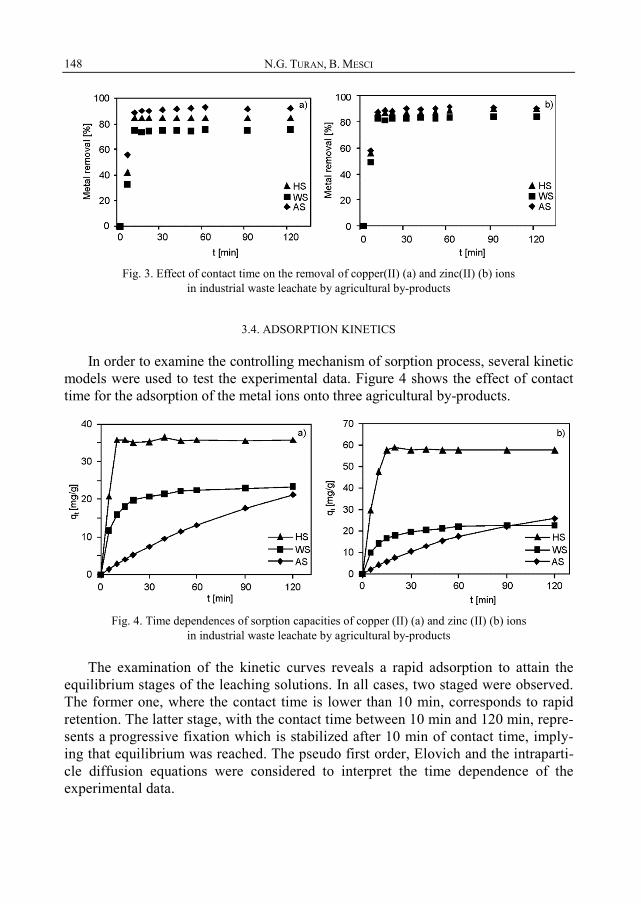
N.G. TURAN, B. MESCI 148
Fig. 3. Effect of contact time on the removal of copper(II) (a) and zinc(II) (b) ions
in industrial waste leachate by agricultural by-products
3.4. ADSORPTION KINETICS
In order to examine the controlling mechanism of sorption process, several kinetic models were used to test the experimental data. Figure 4 shows the effect of contact time for the adsorption of the metal ions onto three agricultural by-products.
Fig. 4. Time dependences of sorption capacities of copper (II) (a) and zinc (II) (b) ions
in industrial waste leachate by agricultural by-products
The examination of the kinetic curves reveals a rapid adsorption to attain the equilibrium stages of the leaching solutions. In all cases, two staged were observed. The former one, where the contact time is lower than 10 min, corresponds to rapid retention. The latter stage, with the contact time between 10 min and 120 min, repre-sents a progressive fixation which is stabilized after 10 min of contact time, imply-ing that equilibrium was reached. The pseudo first order, Elovich and the intraparti-cle diffusion equations were considered to interpret the time dependence of the experimental data.

Adsorption of copper(II) and zinc(II) ions by various agricultural by-products 149
PSEUDO FIRST ORDER KINETIC MODEL
A widely used Lagergreen model was employed to study the pseudo first order ki-netics [28]:
( )1t
e tt
dq k q qd
= − (3)
where qe and qt refer to the amounts of heavy metal (mg·g–1) adsorbed at equilibrium time and time t (d) and k1 is the Lagergreen rate constant (d–1), respectively.
The integration of Eq. (3) gives the following expression:
( ) 1 1ln e tq q k t C− = − + (4)
where C1 is the integration constant for the reaction of the first order and
( ) 1ln ln for 0 at 0e t eq q q k t q t− = − = = (5)
The pseudo first order kinetic model considers the rate of occupation of adsorption sites to be proportional to the number of unoccupied sites. A straight line of ln(qe – qt) vs. t indicates the application of the first order kinetic model (Fig. 5). The rate con-stants (k1) are obtained from slope of the plots.
Fig. 5. Pseudo-first order reaction kinetics for the adsorption of copper(II) (a) and zinc(II) (b) ions
PSEUDO SECOND ORDER KINETIC MODEL
Adsorption data was also evaluated according to the pseudo second order kinetic proposed by [28]:
( )22
te t
dq k q qdt
= − (6)

N.G. TURAN, B. MESCI 150
where qe and qt are the amounts of heavy metal (mg·g–1) adsorbed at equilibrium time and time t (d), respectively, and k2 is the second order reaction constant (g·mg–1·d–1). Integration of Eq. (6) leads to the following expression:
2 2e t
1 k t Cq q
= +−
(7)
In Equation (7), C2 is the integration constant of the second order reaction kinetic. After rearrangement, the following equation is obtained:
2t 2 e e
t 1 1 q k q q
= + (8)
A straight line of t/qt vs. t indicates the application of the second order kinetic model (Fig. 6). The values of k2 are determined from the slope of the plots.
Fig. 6. Pseudo-second order reaction kinetics for the adsorption of copper(II) ions (a) and zinc(II) (b) ions
ELOVICH MODEL
The Elovich equation has the form [29]:
( )exptt
dq qdt
α β= − (9)
where α is the initial adsorption rate (mg·g–1·min–1) and β is the desorption constant (g·mg–1). To simplify the Elovich equation, Chien and Clayton [30] assumed αβt >>1, and for the boundary conditions qt = 0 at t = 0 and qt = qt at t = t, we arrive at [31]:
( )t1 1ln ln q tαββ β
= + (10)
A straight line plot of qt vs. lnt indicates the application of Elovich model (Fig. 7). The values of constants can be obtained from the slopes and intercepts of the plots.

Adsorption of copper(II) and zinc(II) ions by various agricultural by-products 151
Fig. 7. Elovich kinetics for the adsorption of copper(II) (a) and zinc(II) (b) ions
INTRAPARTICLE DIFFUSION MODEL
Transport of the adsorbate from the solution to the surface of the adsorbent parti-cles occurs in several steps. Generally, the process is diffusion controlled, if its rate is dependent on the rate at which components diffuse towards one another. The possibil-ity of intraparticle diffusion was explored by using the intraparticle diffusion model as follows [32]:
1/ 2 t idq K t C= + (11)
where Kid is the intraparticle diffusion rate constant (mg·g–1·min–1/2) and C is the inter-cept. Values of C give an idea about thickness of the boundary layer, i.e., the larger intercept, the greater the boundary layer effect is [7].
Fig. 8. Intraparticle diffusion kinetics for the adsorption of copper(II) (a) and zinc(II) (b) ions
The plot of qt versus t1/2 indicates the application of the intraparticle diffusion model. The values of Kid were determined from the slope of the plots. If the intraparti-cle diffusion is involved in the adsorption process, the plot of the amount of heavy metal adsorbed per unit mass of adsorbent (qt) against square root of time (t1/2) formed a straight line. The particle diffusion would be the controlling step if the line inter-

N.G. TURAN, B. MESCI 152
sected the origin [33]. Figure 8 presents the plots of the amount of Cu(II) and Zn(II) ions adsorbed per unit mass of the adsorbent vs. t1/2. The deviation of straight lines from the origin indicates that intraparticle transport is not the rate limiting step. As seen from Fig. 7, the intraparticle diffusion rate equation fits well to the initial stages of the adsorption process for all the tested metal ions with the agricultural by-products.
The kinetic parameters of Cu(II) and Zn(II) ions onto agricultural by-products (Table 1) were calculated from the plots.
T a b l e 1
Kinetic parameters of adsorption of copper(II) and zinc(II) in leaching solution of industrial waste by agricultural by-productsa
Kinetic equationand parameter HS WS AS Kinetic equation
and parameter HS WS AS
Cu(II) Zn(II) First order kinetic equation
k1 [min–1] 0.046 0.067 0.057 k1 [min–1] 0.040 0.050 0.046 q1 [mg·g–1] 46.512 73.259 70.401 q1 [mg·g–1] 77.254 68.252 73.215 R2 0.975 0.927 0.913 R2 0.975 0.906 0.924
Second order kinetic equation k2 [g·mg–1·min–1] 0.037 0.010 0.968 k2 [g·mg–1·min–1] 0.014 0.008 1.766 q2 [mg·g–1] 35.842 23.981 54.645 q2 [mg·g–1] 58.480 23.641 50.000 R2 0.999 0.999 0.999 R2 0.999 0.997 0.999
Elovich equation α [mg·g–1·min–1] 30.239 9.462 12.215 α [mg·g–1·min–1] 35.456 9.462 15.336 β [g·mg–1] 0.148 0.210 0.229 β [g·mg–1] 0.086 0.207 0.183 R2 0.710 0.927 0.799 R2 0.780 0.960 0.843
Intraparticle diffusion equation Kid [mg·g–1·min–1/2] 2.363 1.835 2.076 Kid [mg·g–1·min–1/2] 4.182 1.895 2.550 R2 0.462 0.729 0.965 R2 0.533 0.786 0.979
aHS– hazelnut shells, WS – walnut shells, AS – almond shells. It can be easily seen from Table 1 that the correlation coefficients (R2) for the
pseudo-second order kinetic model is much higher than the corresponding values of the other kinetic models. Moreover, the calculated qe values are agree with experimen-tal qe values for the pseudo-second order kinetic model, pointing to the applicability of this model to description of the adsorption model.
3.5. FITTING THE POLYNOMIAL EQUATIONS AND STATISTICAL ANALYSIS
In Table 2, the effect of initial pH is presented and basic statistical solutions and experimental ranges of the removal capacities for the use of hazelnut (HS), almond (AS) and walnut shells (WS) are given for further analysis.

Adsorption of copper(II) and zinc(II) ions by various agricultural by-products 153
T a b l e 2
One factor experimental design and its related descriptive statistics for the effect of initial pHa
Adsorbent Responses Min Max AverageRem [%]
Std Rem [%] R
HS removal of Cu(II) 21.2 90.91 71.90 25.53 4.28 HS removal of Zn(II) 27.5 83.43 66.79 19.43 3.03 WS removal of Cu(II) 18.4 80.6 59.88 23.60 4.38 WS removal of Zn(II) 23.4 78.8 60.05 18.77 3.36 AS removal of Cu(II) 45.5 90.8 74.65 15.95 2.04 AS removal of Zn(II) 35.4 93.4 77.07 21.57 2.63
aNumber of run – 7, range – 2–8, Min – minimum value, Max – maximum value, Std – standard deviation, R – the ratio of Max/Min. If R >10, a transformation such as square root, natural log, base 10log, inverse square, etc. is usually required for ANOVA.
T a b l e 3
One factor experimental design and its related descriptive statistics for the effect of adsorbent dosagea
Adsorbent Responses Min Max AverageRem [%]
Std Rem [%] R
HS removal of Cu(II) 45.55 92.21 74.74 19.12 2.02HS removal of Zn(II) 37.67 81.21 62.79 17.68 2.15WS removal of Cu(II) 30.21 78.55 55.71 19.35 2.60WS removal of Zn(II) 28.90 70.41 51.27 17.25 2.43AS removal of Cu(II) 40.20 89.70 67.90 20.65 2.23AS removal of Zn(II) 35.40 85.20 61.78 20.56 2.40aNumber of run – 5, range – 2–10.
T a b l e 4
One factor experimental design and its related descriptive statistics for the effect of contact timea
Adsorbent Responses Min Max AverageRem [%]
Std Rem [%] R
HS removal of Cu(II) 41.80 84.90 80.39 13.56 2.03HS removal of Zn(II) 55.60 90.30 84.72 10.33 1.62WS removal of Cu(II) 33.20 75.50 70.49 13.11 2.27WS removal of Zn(II) 48.88 84.20 79.61 10.82 1.72AS removal of Cu(II) 55.60 92.90 87.76 11.36 1.67AS removal of Zn(II) 58.24 91.88 86.71 10.07 1.57aNumber of run – 10, range – 5–120.

N.G. TURAN, B. MESCI 154
In Table 3, the effect of adsorbent dosage is shown and basic statistical solutions and experimental ranges of the removal capacities for t HS, AS and WS are given for further analysis. Similarly, in Table 4, the effect of contact time is presented and basic statistical solutions and experimental ranges of the removal capacities for the adsorb-ents used are given for further analysis. The experiments are repeated as twice to in-crease the reliability and average values of removal capacities are used for analysis.
In order to make a decision which of various models (linear, quadratic, or cubic) is better to describe removal capacities of Cu(II) and Zn(II) ions by HS, AS and WS, statistical calculations were carried out. Their results are given in Tables 5–7.
T a b l e 5
Model summary statistics of HS for selecting the adequacy of the models
The effect of initial pH
Removal of Cu(II) Removal of Zn(II)
Source Std. Dev R2 Adju. R2 Pre. R2 PRESS Std. Dev R2 Adj. R2 Pre. R2 PRESS Linear 13.25 0.7757 0.7308 0.3965 2360.70 9.45 0.8028 0.7634 0.4440 1259.36 Quadratic 4.90 0.9755 0.9632 0.8430 614.09 5.52 0.9462 0.9194 0.6633 762.65 Cubic 2.11 0.9966 0.9932 0.9543 178.67 3.73 0.9815 0.9630 0.5601 996.51 Quartic 1.67 0.9986 0.9957 0.9541 179.64 1.05 0.9990 0.9971 0.8886 252.32 Fifth 2.23 0.9987 0.9924 –1.419 9465.01 0.77 0.9997 0.9984 0.4965 1140.50
The effect of adsorbent dosage
Removal of Cu(II) Removal of Zn(II)
Source Std. Dev R2 Adj. R2 Pre. R2 PRESS Std. Dev R2 Adj. R2 Pre. R2 PRESS Linear 6.22 0.9205 0.8941 0.6482 514.71 3.59 0.9692 0.9589 0.8637 170.39 Quadratic 0.81 0.9991 0.9982 0.9940 8.75 0.75 0.9991 0.9982 0.9893 13.40 Cubic 1.09 0.9992 0.9968 0.8781 178.27 0.72 0.9996 0.9983 0.9376 78.02
The effect of contact time
Removal of Cu(II) Removal of Zn(II)
Source Std. Dev R2 Adj. R2 Pre. R2 PRESS Std. Dev R2 Adj. R2 Pre. R2 PRESS Linear 13.32 0.1417 0.0344 –0.451 2401.66 9.57 0.2370 0.1416 –0.306 1254.85 Quadratic 12.62 0.3260 0.1334 –1.032 3362.97 9.04 0.4044 0.2342 –0.686 1619.77 Cubic 11.64 0.5086 0.2630 –8.309 15405.9 8.58 0.5401 0.3102 –7.399 8067.66 Quartic 9.71 0.7149 0.4868 –140.8 2.347E5 7.21 0.7291 0.5123 –143.0 1.384E5 Fifth 7.38 0.8685 0.7042 –2681 4.439E6 5.31 0.8826 0.7357 –2310 2.220E6 Sixth 5.33 0.9486 0.8457 3.92 0.9520 0.8559

Adsorption of copper(II) and zinc(II) ions by various agricultural by-products 155
Values corresponding to suggested models are underlined in the tables. The effect of initial pH can be modelled as cubic for HS, cubic for AS and quadratic for WS for removal of Cu(II) ions. Similarly, the effect of initial pH can be modelled as quartic for HS, cubic for AS and cubic for WS for removal of Zn(II) ions. The effect of ad-sorbent dosage can be modelled as quadratic for HS, linear for AS and linear for WS for removal of Cu(II) ions. Similarly, the effect of adsorbent dosage can be modelled as quadratic for HS, linear for AS and linear for WS for removal of Zn(II) ions. The effect of contact time can be modelled as fifth for HS, fifth for AS and fifth for WS for removal of Cu(II). Similarly, the effect of contact time can be modelled as fifth for HS, fifth for AS and fifth for WS for removal of Zn(II).
T a b l e 6
Model summary statistics of AS for selecting the adequacy of the models
The effect of initial pH
Removal of Cu(II) Removal of Zn(II)
Source Std. Dev R2 Adj. R2 Pre. R2 PRESS Std. Dev R2 Adj. R2 Pre. R2 PRESS Linear 6.08 0.8790 0.8548 0.6749 496.62 10.61 0.7986 0.7583 0.4656 1492.57 Quadratic 3.48 0.9684 0.9225 0.8138 284.40 2.92 0.9878 0.9817 0.9201 223.19 Cubic 1.76 0.9939 0.9878 0.8716 196.10 1.17 0.9985 0.9971 0.9938 17.34 Quartic 1.20 0.9981 0.9943 0.7429 392.78 1.32 0.9988 0.9963 0.9771 64.05 Fifth 0.56 0.9998 0.9988 0.6044 604.40 1.86 0.9988 0.9926 –1.362 6598.20
The effect of adsorbent dosage
Removal of Cu(II) Removal of Zn(II)
Source Std. Dev R2 Adj. R2 Pre. R2 PRESS Std. Dev R2 Adj. R2 Pre. R2 PRESS Linear 3.73 0.9755 0.9674 0.9019 167.34 2.59 0.9881 0.9841 0.9602 67.26 Quadratic 2.92 0.9900 0.9800 0.8693 222.90 2.76 0.9910 0.9819 0.8866 191.84 Cubic 2.45 0.9965 0.9859 0.4696 904.70 2.46 0.9964 0.9857 0.4601 913.55
The effect of contact time
Removal of Cu(II) Removal of Zn(II)
Source Std. Dev R2 Adj. R2 Pre. R2 PRESS Std. Dev R2 Adj. R2 Pre. R2 PRESS Linear 10.85 0.1887 0.0873 –0.391 1616.57 9.59 0.1944 0.0937 –0.398 1277.92 Quadratic 9.92 0.4072 0.2379 –0.891 2196.80 8.70 0.4208 0.2553 –0.767 1615.94 Cubic 8.96 0.5853 0.3780 –6.333 8519.25 8.00 0.5801 0.3701 –6.532 6885.59 Quartic 7.61 0.7505 0.5508 –129.6 1.518E5 6.74 0.7518 0.5532 –139.3 1.283E5 Fifth 5.62 0.8911 0.7549 –2311 2.686E6 4.82 0.8985 0.7716 –1846 1.689E6 Sixth 3.96 0.9596 0.8788 3.69 0.9554 0.8662

N.G. TURAN, B. MESCI 156
T a b l e 7
Model summary statistics of WS for selecting the adequacy of the models
The effect of initial pH
Removal of Cu(II) Removal of Zn(II) Source Std. Dev R2 Adj. R2 Pre. R2 PRESS Std. Dev R2 Adj. R2 Pre. R2 PRESS
Linear 9.56 0.8632 0.8358 0.6697 1103.84 7.93 0.8514 0.8217 0.5941 858.05 Quadratic 2.34 0.9934 0.9901 0.9737 87.87 4.65 0.9591 0.9387 0.7148 602.86 Cubic 2.47 0.9945 0.9891 0.8660 447.65 2.52 0.9910 0.9819 0.8581 300.06 Quartic 1.09 0.9993 0.9979 0.9279 240.84 2.42 0.9945 0.9834 0.4373 1189.68 Fifth 0.94 0.9997 0.9984 0.4941 1690.68 2.08 0.9979 0.9877 –2.9174 8282.02
The effect of adsorbent dosage
Removal of Cu(II) Removal of Zn(II) Source Std. Dev R2 Adj. R2 Pre. R2 PRESS Std. Dev R2 Adj. R2 Pre. R2 PRESS Linear 2.67 0.9857 0.9810 0.9661 50.81 2.50 0.9842 0.9790 0.9436 67.19
Quadratic 2.34 0.9927 0.9854 0.9598 60.30 2.46 0.9898 0.9796 0.8644 161.52 Cubic 3.28 0.9928 0.9713 –0.079 1618.58 2.01 0.9966 0.9864 0.48880 609.77
The effect of contact time
Removal of Cu(II) Removal of Zn(II) Source Std. Dev R2 Adj. R2 Pre. R2 PRESS Std. Dev R2 Adj. R2 Pre. R2 PRESS Linear 12.79 0.1548 0.0492 –0.4262 2209.11 10.42 0.1770 0.0741 –0.4041 1481.94
Quadratic 12.18 0.3291 0.1374 –1.0085 3111.19 9.80 0.3636 0.1818 –0.8699 1973.57 Cubic 11.31 0.5042 0.2563 –7.9652 13886.9 9.12 0.5273 0.2910 –8.2769 9791.31
Quartic 9.59 0.7034 0.4661 –144.50 2.254E5 7.56 0.7295 0.5130 –122.84 1.307E5 Fifth 7.41 0.8584 0.6814 –2352.1 3.645E6 6.00 0.8633 0.6925 –2313.8 2.443E6 Sixth 5.93 0.9319 0.7956 4.78 0.9352 0.8055
An empirical relationship expressed by polynomial equations with the main ef-
fects (known as input variables) was fitted between the experimental results and the input variables. The final equations obtained in terms of actual factors as follows:
• The use of HS:
2 3Cu(II) 99.83 82.95 12.32 0.61Y A A A= − + − + (12)
2 3 4Zn(II) 186.76 188.75 52.65 6.52 0.29Y A A A A= − + − + − (13)
2Cu(II) 19.87 14.39 0.71Y B B= + − (14)
2Zn(II) 18.32 10.40 0.40Y B B= + − (15)
2 3 5 4 7 5Cu(II) 0.86 11.64 0.53 0.01 9.53 3.06Y C C C C C− −= + − + + + (16)
2 3 3 5 4 7 5Zn(II) 25.24 8.62 0.40 8.12 7.24 2.33Y C C C C C− − −= + + + − + (17)

Adsorption of copper(II) and zinc(II) ions by various agricultural by-products 157
• The use of AS:
2 3Cu(II) 24.99 48.57 7.65 0.42Y A A A= − + − + (18)
2 3Zn(II) 53.72 59.31 8.09 0.37Y A A A= − + − + (19)
Cu(II) 29.20 6.45Y B= + (20)
Zn(II) 22.99 6.46Y B= + (21)
2 3 3 5 4 7 5Cu(II) 22.72 9.28 0.42 8.54 7.61 2.45Y C C C C C− − −= + − + − + (22)
2 3 3 5 4 7 5Zn(II) 28.60 8.32 0.38 7.73 6.89 2.22Y C C C C C− − −= + − + − + (23)
• The use of WS:
2Cu(II) 38.66 32.91 2.27Y A A= − + − (24)
2 3Zn(II) 64.85 62.44 10.02 0.55Y A A A= − + − + (25)
Cu(II) 19.24 6.07Y B= + (26)
Zn(II) 51.27 21.65Y B= + (27)
2 3 5 4 7 5Cu(II) 5.94 11.20 0.51 0.01 9.28 2.97Y C C C C C− −= − + − + − + (28)
2 3 3 5 4 7 5Zn(II) 17.76 8.89 0.40 8.09 7.14 2.28Y C C C C C− − −= + − + − + (29)
In Equations (12)–(29), the coefficients A, B and C represent the effect of initial pH, adsorbent dosage and contact time, respectively.
Based on the R2 value, the performance of the fitted curves is almost near the per-formance of the second order kinetic equation. Equations (20), (21), (26), and (27) are only expressed by linear regression. These equations occur in a linear form due to the PRESS value (abbr. prediction error sum of squares). As seen in Table 6 and 7, the PRESS values of these equations are smaller than of other ones. The statistical signifi-cance of the ratio of mean square variation due to regression and mean square residual error was tested by the ANOVA method. The results showed that the equations ade-quately represented the actual relationship between the response and significant vari-ables. The values of initial pH, adsorbent dosage and contact time are optimized by the Simplex algorithm [34]. The optimized values are presented in Table 8. Table 9 and 10 present the comparison of biosorption capacity (mg/g) of HS, WS, AS biomass from the Elovich isotherm for Cu(II) and Zn(II) with that of various biomass reported in literature.

N.G. TURAN, B. MESCI 158
T a b l e 8
Optimized values of initial pH, adsorbent dosage and contact time
Agricultural by-products Removal efficiency [%]
Cu(II) Zn(II) The use of AS
Initial pH 6.29 80.81 88.75 Adsorbent dosage 8.21 mg/dm3 79.47 69.59 Contact time 15.41 min 93.61 91.88
The use of HS Initial pH 6.85 87.45 75.71 Adsorbent dosage 8.77 mg/dm3 88.49 74.52 Contact time 15.99 min 89.38 90.3
The use of WS Initial pH 6.53 73.74 68.44 Adsorbent dosage 8.10 mg/dm3 69.51 65.05 Contact time 15.67 min 76.77 84.20
T a b l e 9
Biosorption capacities of various biosorbents for Cu(II) removal
Biosorbent qmax [mg·g–1] ReferenceHazelnut shells 35.61 this studyAlmond shells 23.35 this studyWalnut shells 21.28 this studyPeanut shells 25.4 [11] Hyacinth roots 22.7 [35] Crab shell biomass 38.62 [36] Arca shell biomass 17.64 Fungal biomass Botrytis cinerea 9.23 [37] Wheat shell 8.34 [38] Cone biomass Thuja orientalis 19.23 [39] Orange residue 23.47 [40] Pinus silvestris biomass 28.83 [41] Sawdust 4.9
[42] Brown alga Fucus vesiculosus 23.4 Terrestrial moss Pleurozium schreberi 11.1 Sugar beet pulp 31.4 [43] Herbaceous 4.84 [44] Dehydrated wheat bran 51.5 [45] Wheat straw 4.48
[46] Soybean straw 5.44 Crab shell 44.94 Rice bran 27.81 Focus vesiculosus 23.4 [42] Arca shell 26.88

Adsorption of copper(II) and zinc(II) ions by various agricultural by-products 159
T a b l e 10
Biosorption capacities of various biosorbents for Zn(II) removal
Biosorbent qmax [mg·g–1] ReferenceHazelnut shells 57.69 this studyAlmond shells 22.6 this studyWalnut shells 25.7 this studyPadina sp. 35.1 [47] Sargassum sp. 29.8 Laminaria hyperborea 19.2 [48] Sargassum muticum 34.1 [49] Fucus spiralis 34.3 [50] Bifurcaria bifurcata 30.3 Ceratophyllum demersum 13.98 [51] Fontinalis antipyretica 15 [52] Cork (C0 = 10 mg/dm3) 3.4
[53] Cork (C0 = 70 mg/dm3) 7.5 Cork (C0 = 150 mg/dm3) 12,4 Myriophyllum spicatum 15.59 [54] Streptomyces noursei 1.6 [55] Chlorella kessleri (C0 = 9 mg/dm3) 4.15
[56] Chlorella kessleri (C0 = 68 mg/dm3) 20.53 Chlorella kessleri (C0 = 150 mg/dm3) 40.38
4. CONCLUSIONS
The study revealed that agricultural by-products such as hazelnut, walnut and al-mond shells, could be used to remove copper(II) and zinc(II) ions from aqueous leachate of industrial waste.
The adsorption of copper(II) and zinc(II) ions on the agricultural by-products is found to be pH, contact time and adsorbent dosage dependent. The maximum adsorp-tion capacity of agricultural by-products was obtained at pH 6 for copper(II) and at pH 8 for zinc(II) ions. The amount of copper(II) and zinc(II) ions removed increased upon increasing the agricultural by-product dosages.
The equilibrium established within the first 10 min. The pseudo second order ki-netic model agrees very well with the dynamic behaviour of the adsorption of cop-per(II) and zinc(II) ions from aqueous leachate of industrial waste onto agricultural by-products.
The shells under investigation had relatively high capacities for the removal of copper(II) and zinc(II) ions from aqueous leachate of industrial waste. Furthermore, as seen from Tables 9 and 10, the removal efficiencies of the proposed agricultural by products are higher than those of various bio-sorbents reported in the literature.

N.G. TURAN, B. MESCI 160
REFERENCES
[1] FERNÁNDEZ Y., MARAÑÓN E., CASTRILLÓN L., VÁZQUEZ I., J. Hazar. Mat., 2005, 126, 169. [2] ŚLĘZAK R., KRZYSTEK L., LEDAKOWICZ S., Environ. Prot. Eng., 2009, 35 (3), 81. [3] BOHDZIEWICZ J., KWARCIAK A., NECZAJ E., Environ. Prot. Eng., 2005, 31 (3-4), 61. [4] BILGILI M.S., DEMIR A., �NCE M., ÖZKAYA B., J. Hazar. Mater., 2007, 145, 186. [5] RODRÍGUEZ J., CASTRILLÓN L., MARAÑÓN E., SASTRE H., FERNÁNDEZ E., Water Resour., 2004, 38,
3297. [6] GUPTA V.K., SHRIVASTAVA A.K., JAIN N., Water Resour., 2001, 35, 4079. [7] EL-ASHTOUKHY E.-S.Z., AMIN N.K., ABDELWAHAB O., Desalination, 2008. 223, 162. [8] JAIN C.K., SINGHAL D.C., SHARMA M.K., J. Hazar. Mater., 2004, 114, 231. [9] SÖLENER M., TUNALI S., ÖZCAN A.S., ÖZCAN A., GEDIKBEY T., Desalination, 2008, 223, 308.
[10] WAFWOYO W., SEO C.W., MARSHALL S.E., J. Chem. Technol. Biotechnol., 1999, 74, 1117. [11] WITEK-KROWIAK A., SZAFRAN R.G., MODELSKI S., Desalination, 2011, 265(1-3), 126. [12] CIMINO G., PASSERINI A., TOSCANO G., Water Resour., 2000, 34, 2955. [13] LOW K.S., LEE C.K., LEO A.C., Biores. Technol., 1995, 51, 227. [14] HO Y.S., MCKAY G., Water Resour., 2000, 34, 735. [15] POOTS V.J.P., MC KAY G., HEALY J.J., J. Water Pollut. Control Feder., 1978, 50, 926. [16] AL-ASHEH S., DUVNJAK Z., Adv. Environ. Res., 1997, 2, 194. [17] MARSHALL W.E., JOHNS M.M., J. Chem. Technol. Biotechnol., 1996, 66, 192. [18] MISHRA S.P., TIWARI D., DUBEY R.S., Appl. Radiat. Isotopes., 1997, 48, 877. [19] YU B., ZHANG Y., SHUKLA A., SHUKLA S.S., DORRIS K.L., J. Hazar. Mater., 2000, 84, 83. [20] BALKÖSE D., BALTACIOĞLU H., J. Chem. Technol. Biotechnol., 1992, 54, 393. [21] AZAB M.S., PETERSON P.J., Water Sci. Technol., 1989, 21, 1705. [22] ZAGGOUT F.R., Asian J. Chem., 2001, 13, 639. [23] DANG V.B.H., DOAN H.D., DANG-VU T., LOHI A., Biores. Technol., 2009, 100, 211. [24] Shake Extraction of Solid Waste with Water, Am. Soc. Test. Mater., ASTM 3987-85, [In:] Annual
Book of ASTM Standards, West Conshohocken, 1990, PA. [25] LOW K.S., LEE C.K., LEE K.P., Biores. Technol., 1993, 44, 109. [26] DORRLS K.L., YU B., ZHANG Y., SHUKLA A., SHUKLA S.S., J. Hazar. Mater., 2000, 80, 33. [27] BULUT Y., TEZ Z., J. Hazar. Mater., 2007, 149, 35. [28] HO Y.S., Scientometrics, 2004, 59, 171. [29] LOW M.J.D., Chem. Rev., 1960, 6, 267. [30] CHIEN S.H., CLAYTON W.R., Soil Sci. Soc. Am. J., 1980, 44, 265. [31] SPARKS D.L., Kinetics and Mechanisms of Chemical Reactions at the Soil Mineral/Water Interface,
[In:] Soil Physical Chemistry, CRC Press, Boca Raton, 1999, Florida. [32] SRIHARI V., DAS A., Desalination, 2008, 225, 220. [33] AL-ASHEH S., BANAT F., ABU-AITAH L., Sep. Purif. Technol., 2003, 33, 1. [34] CHVATAL V., Linear Programming, W.H. Freeman Comp., New York, 1983. [35] ZHENG J.-C., FENG H.-M., LAM M.H.-W., J. Hazar. Mater., 2009, 171, 780. [36] DAHIYA S., TRIPATHI R.M., HEGDE A.G., J. Hazar. Mater., 2008, 150, 376. [37] AKAR T., TUNALI S., MIneral. Eng., 2005, 18, 1099. [38] BASCI N., KOCADAGISTAN E., KOCADAGISTAN B., Desalination, 2004, 164, 135. [39] NUHOGLU Y., OGUZ E., Process Biochem., 2003, 38, 1627. [40] KHORMAEI M., NASERNEJAD B., EDRISI M., J. Hazar. Mater., 2007, 149, 269. [41] UCUN H., AKSAKAL O., YILDIZ E., J. Hazar. Mater., 2009, 161, 1040. [42] GRIMM A., ZANZI R., BJÖRNBOM E., Bioresour. Technol., 2008, 99, 2559. [43] ZÜMRIYE AKSU Z., ISAOĞLU I.A., Process Biochem., 2005,40, 3031.

Adsorption of copper(II) and zinc(II) ions by various agricultural by-products 161
[44] GÜNDOGAN R., ACEMIOGLU B., ALMA M.H., J. Colloid Interface Sci., 2004, 269, 303. [45] ÖZER A., ÖZER D., ÖZER A., Process Biochem., 2004, 39, 2183. [46] SCIBAN M., KLASNJA M., SKRBIC B., Desalination, 2008, 229, 170. [47] SHENG P.X., TING Y.P., CHEN P., HONG L., J. Colloid Interface Sci., 2004, 275, 131. [48] PURANIK P.R., PAKNICAR K.M., Bioresour. Technol., 1999, 70, 269. [49] YU Q., MATHEICKAL J.T., YIN P., KAEWSARN P., Water Res., 1999, 33(6), 1534. [50] PRASAD M.N.V., FREITAS H., Environ. Pollut., 2000, 110, 277. [51] KESKINKAN O., GOKSU M.Z.L., BASIBUYUK M., FORSTER C.F., Biores. Technol., 2004, 92, 197. [52] MARTINS R.J.E., PARDO R., BOAVENTURA R.A.R., Water Res., 2004, 38, 693. [53] CHUBAR N., CARVALHO J.R., CORREIA M.J.N., Physicochem. Eng. Aspects, 2004, 230, 57. [54] KESKINKAN O., GOKSU M.Z.L., YUCEER A., BASIBUYUK M FORSTER C.F., Process Biochem., 2003,
39, 179. [55] RUIZ C.G., TIRADO V.R., GIL B.G., Biores. Technol., 2008, 99, 3864. [56] HORVATHOVA H., MRAZIKOVA A., KADUKOVA J., STOFKO M., Zinc Removal from Model Solution by
Biosorption, 4th European Bioremediation Conference, Chania, Crete, Greece, September 3–8, 2008.