4. TIDES

4.1 INTRODUCTION

This chapter provides background information on the tidal data in Chapter 9 of this Almanac, where times and heights of HW and LW are shown for Standard Ports, and time and height differences for their associated Secondary Ports. Tides are predicted for average meteorological conditions. In the UK the average pressure is about 1013mb. A difference of 34mb can cause the tide to rise (lower pressure) or fall (higher pressure) by about 0·3m. See 4.8 for more details.

4.1.1 Admiralty Tide Tables (ATT)

are the source for all tidal data in this Almanac; they are published in 4 volumes:

● Vol 1 (NP•201) UK and Ireland (including Channel ports from Hoek van Holland to Brest);● Vol 2 (NP•202) Europe (excluding UK, Ireland and Channel ports), Mediterranean and the Atlantic;● Vol 3 (NP•203) Indian Ocean and South China Sea;● Vol 4 (NP•204) Pacific•Ocean.

4.1.2 Spanish Secondary Ports referenced to Lisboa

In Areas 23 and 25, some Spanish secondary ports have Lisboa as Standard Port. Time differences for these ports, when applied to the printed times of HW and LW for Lisboa (UT), automatically give HW and LW times in the Zone Time for Spain (ie UT –1), not Portugal (UT). No other corrections are required, except for DST when applicable.

4.2 DEFINITIONS

Chart Datum (CD) CD is the reference level from which heights of tide are predicted and charted depths are measured. In the UK it normally approximates to LAT, and the tide will not frequently fall below it. The actual depth of water in any particular position is the charted depth plus the height of tide. Lowest Astronomical Tide (LAT) LAT is the lowest level which can be predicted under average meteorological, and any combination of astronomical, conditions. This level will not be reached every year. Storm surges can cause even lower levels to be reached. Highest Astronomical Tide (HAT) HAT is the highest level which can be predicted to occur under average meteorological conditions and under any combination of astronomical conditions, except storm surges. It is the level above which vertical clearances under bridges and power lines are measured; see 4.5. Ordnance Datum (Newlyn) Ordnance Datum (Newlyn) is the datum of the land levelling system on mainland England, Scotland and Wales, and to which all features on UK land maps are referred. The difference between Ordnance Datum (Newlyn) and CD is shown at the foot of each page of tide tables in this Almanac. Differences between CD and foreign land levelling datums are similarly quoted. Charted depth Charted depths are printed on charts in metres and decimetres (0·1m) and show the depth of water below CD. (Not to be confused with a sounding which is the actual depth of water (charted depth + height of tide) in a particular position.) Drying height

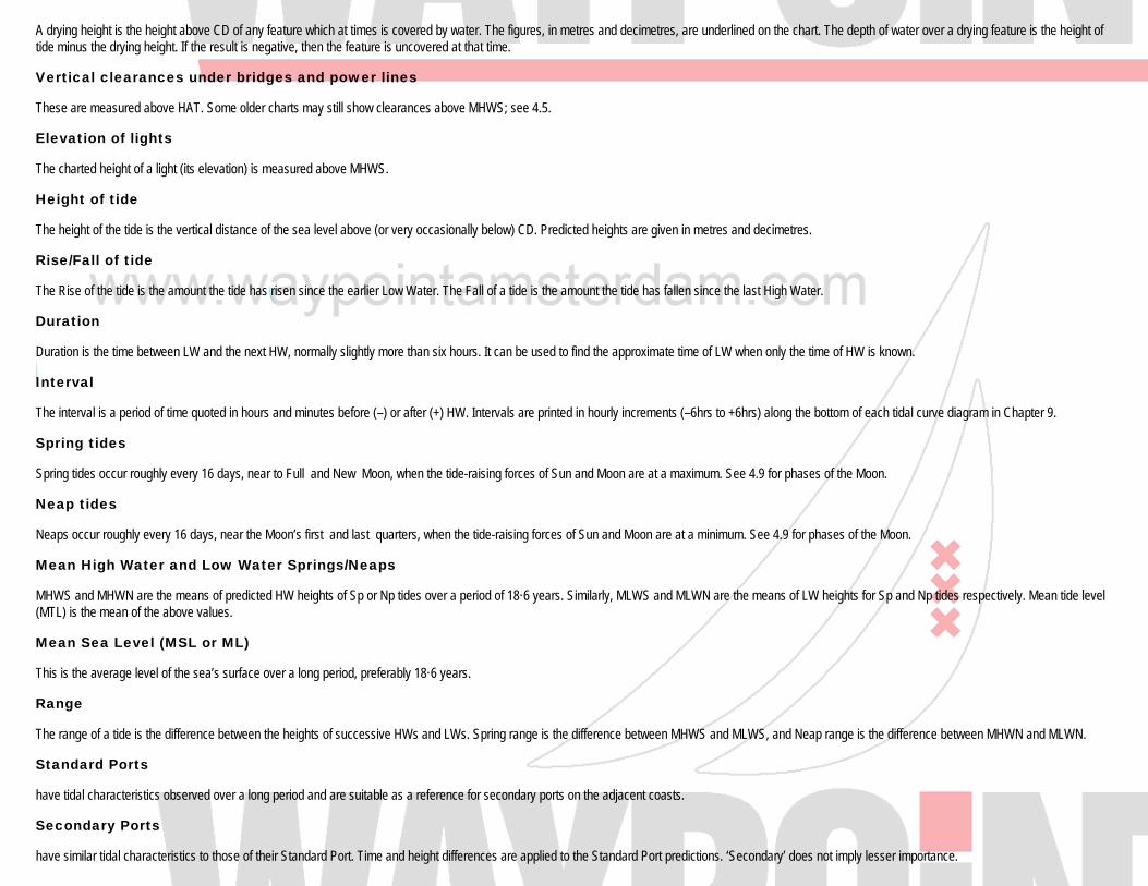
A drying height is the height above CD of any feature which at times is covered by water. The figures, in metres and decimetres, are underlined on the chart. The depth of water over a drying feature is the height of tide minus the drying height. If the result is negative, then the feature is uncovered at that time. Vertical clearances under bridges and power lines These are measured above HAT. Some older charts may still show clearances above MHWS; see 4.5. Elevation of lights The charted height of a light (its elevation) is measured above MHWS. Height of tide The height of the tide is the vertical distance of the sea level above (or very occasionally below) CD. Predicted heights are given in metres and decimetres. Rise/Fall of tide The Rise of the tide is the amount the tide has risen since the earlier Low Water. The Fall of a tide is the amount the tide has fallen since the last High Water. Duration Duration is the time between LW and the next HW, normally slightly more than six hours. It can be used to find the approximate time of LW when only the time of HW is known. Interval The interval is a period of time quoted in hours and minutes before (–) or after (+) HW. Intervals are printed in hourly increments (–6hrs to +6hrs) along the bottom of each tidal curve diagram in Chapter 9. Spring tides Spring tides occur roughly every 16 days, near to Full and New Moon, when the tide-raising forces of Sun and Moon are at a maximum. See 4.9 for phases of the Moon. Neap tides Neaps occur roughly every 16 days, near the Moon’s first and last quarters, when the tide-raising forces of Sun and Moon are at a minimum. See 4.9 for phases of the Moon. Mean High Water and Low Water Springs/Neaps MHWS and MHWN are the means of predicted HW heights of Sp or Np tides over a period of 18·6 years. Similarly, MLWS and MLWN are the means of LW heights for Sp and Np tides respectively. Mean tide level (MTL) is the mean of the above values. Mean Sea Level (MSL or ML) This is the average level of the sea’s surface over a long period, preferably 18·6 years. Range The range of a tide is the difference between the heights of successive HWs and LWs. Spring range is the difference between MHWS and MLWS, and Neap range is the difference between MHWN and MLWN. Standard Ports have tidal characteristics observed over a long period and are suitable as a reference for secondary ports on the adjacent coasts. Secondary Ports have similar tidal characteristics to those of their Standard Port. Time and height differences are applied to the Standard Port predictions. ‘Secondary’ does not imply lesser importance.

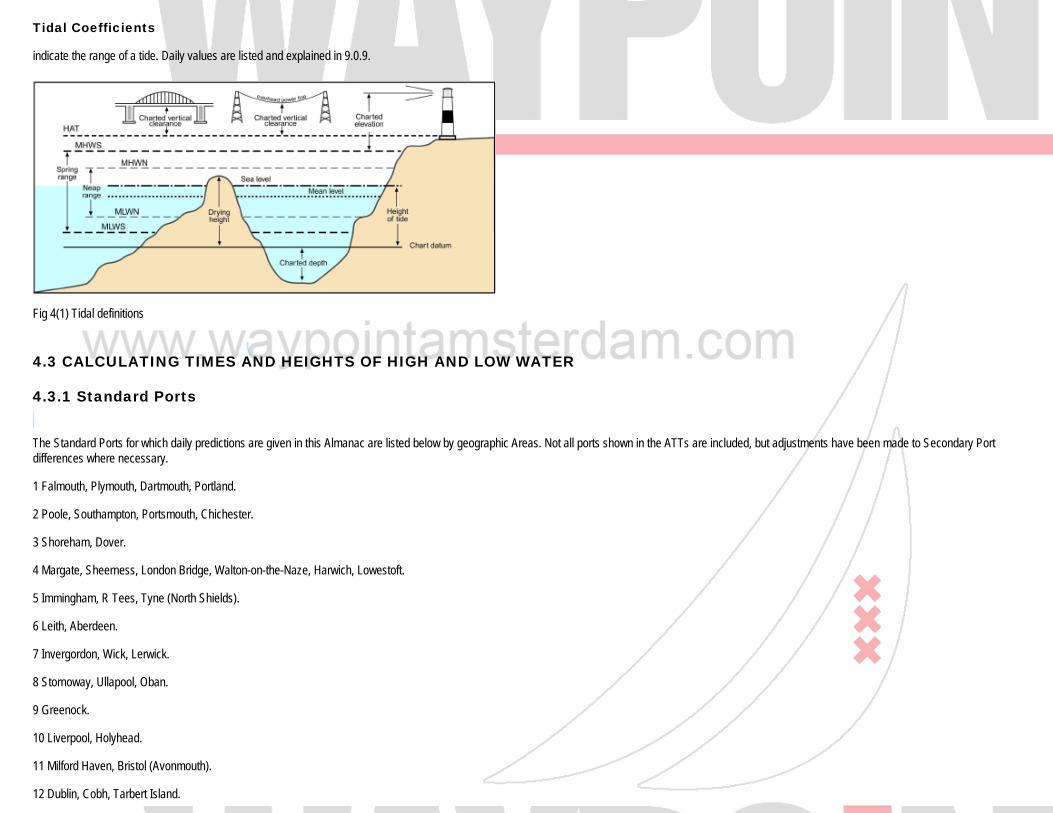
Tidal Coefficients indicate the range of a tide. Daily values are listed and explained in 9.0.9.

Fig 4(1) Tidal definitions

4.3 CALCULATING TIMES AND HEIGHTS OF HIGH AND LOW WATER

4.3.1 Standard Ports

The Standard Ports for which daily predictions are given in this Almanac are listed below by geographic Areas. Not all ports shown in the ATTs are included, but adjustments have been made to Secondary Port differences where necessary. 1 Falmouth, Plymouth, Dartmouth, Portland. 2 Poole, Southampton, Portsmouth, Chichester. 3 Shoreham, Dover. 4 Margate, Sheerness, London Bridge, Walton-on-the-Naze, Harwich, Lowestoft. 5 Immingham, R Tees, Tyne (North Shields). 6 Leith, Aberdeen. 7 Invergordon, Wick, Lerwick. 8 Stornoway, Ullapool, Oban. 9 Greenock. 10 Liverpool, Holyhead. 11 Milford Haven, Bristol (Avonmouth). 12 Dublin, Cobh, Tarbert Island.

13 Galway, River Foyle, Galway. 14 Esbjerg. 15 Helgoland, Cuxhaven and Wilhelmshaven. 16 Hoek van Holland, Vlissingen, Zeebrugge. 17 Dunkerque, Dieppe, Le Havre, Cherbourg. 18 St Malo. 19 St Peter Port, St Helier. 20 Brest. 22 Pointe de Grave. 23 La Coruña. 24 Lisboa. 25 Gibraltar. Predicted times and heights of HW and LW are tabulated for each Standard Port. Note that these are only predictions and take no account of the effects of wind and barometric pressure (see 4.8). See 1.5 for Zone times and Daylight Saving Time (DST).

4.3.2 Secondary Ports – times of HW and LW

Each Secondary Port listed in Chapter 9 has a data block for calculating times of HW and LW. The following example is for Braye (Alderney): TIDES –0400 Dover; ML 3·5; Duration 0545 Standard Port ST HELIER → Times Height (metres) High Water Low Water MHWS MHWN MLWN MLWS 0300 0900 0200 0900 11·0 8·1 4·0 1·4 1500 2100 1400 2100 Differences BRAYE +0050 +0040 +0025 +0105 –4·8 –3·4 –1·5 –0·5 In this example –0400 Dover means that, on average, HW Braye is 4 hours 00 minutes before HW Dover (the Range and times of HW Dover are in Area 3 and on the bookmark). ML (or MSL) is defined in 4.2. Duration 0545 means that LW Braye occurs 5 hours and 45 minutes before the next HW.

The arrow → after the Standard Port’s name points to where the tide tables are in the book. The most accurate method of prediction uses Standard Port times and Secondary Port time differences as in the block. When HW at St Helier occurs at 0300 and 1500, the difference is +•0050, and thus HW at Braye occurs at 0350 and 1550. When HW at St Helier occurs at 0900 and 2100, the difference is +•0040, and HW at Braye occurs at 0940 and 2140. If, as will usually be the case, HW St Helier occurs at some other time, then the difference for Braye must be found by interpolation, either by eye, by the graphical method or by calculator. So when HW St Helier occurs at 1200 (midway between 0900 and 1500), the difference is +•0045 (midway between +0040 and +0050), and therefore HW Braye is 1245. The same method is used for calculating the times of LW. Times thus obtained are in the Secondary Port’s Zone Time. For calculating heights of HW and LW see 4.3.3.

4.3.3 Secondary Ports – heights of HW and LW

The Secondary Port data block also contains height differences which are applied to the heights of HW and LW at the Standard Port. When the height of HW at St Helier is 11·0m (MHWS), the difference is –4·8m, so the height of HW Braye is 6·2m (MHWS). When the height of HW St Helier is 8·1m (MHWN), the difference is –3·4m, and the height of HW at Braye is 4·7m (MHWN). If, as is likely, the height of tide at the Standard Port differs from the Mean Spring or Neap level, then the height difference must also be interpolated: by eye, by graph or by calculator. Thus if the height of HW St Helier is 9·55m (halfway between MHWS and MHWN), the difference is –4·1m, and the height of HW Braye is 5·45m (9·55–4·1m).

4.3.4 Graphical method for interpolating time and height differences

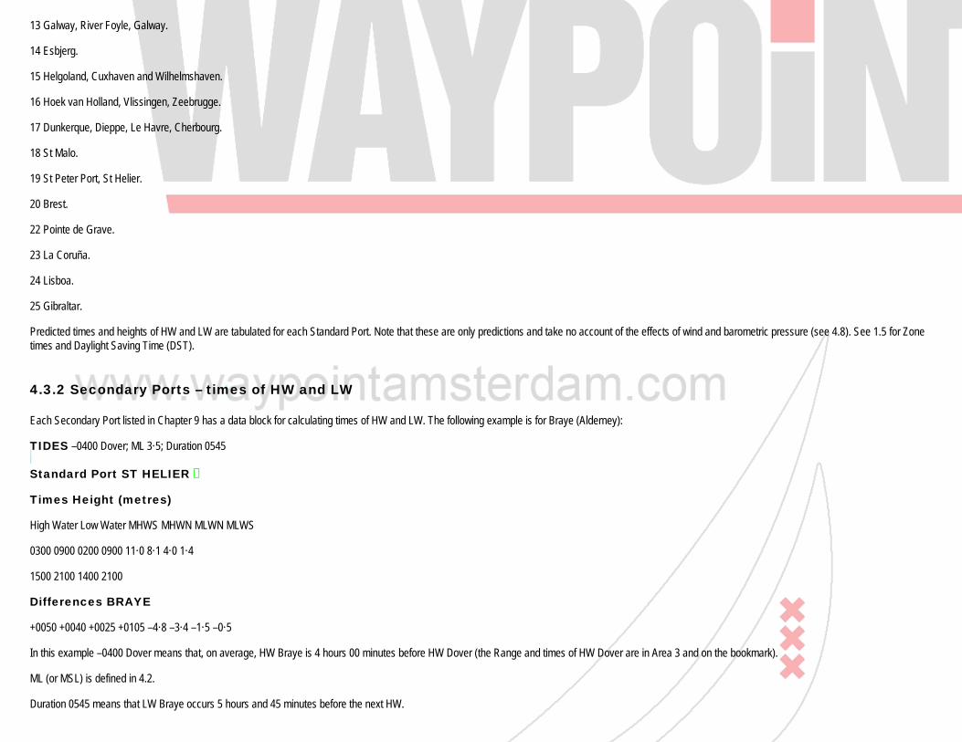
Any suitable squared paper can be used, having chosen convenient scales; see Figs 4(2) and 4(3). Example: using the data for Braye in 4.3.2, find the time and height differences for HW at Braye if HW St Helier occurs at 1126, height 8·9m. Time difference On the horizontal axis of Fig 4(2) select a scale for the time at St Helier covering 0900 to 1500 (for which the relevant time differences for Braye are known). On the vertical axis the scale must cover +0040 to +0050, the time differences given for 0900 and 1500. Plot point A, the time difference (+0040) for HW St Helier at 0900; and point B, the time difference (+0050) for HW St Helier at 1500. Join AB. Enter the graph at time 1126 (HW St Helier); intersect AB at C then go horizontally to read +0044 on the vertical axis. On that morning HW Braye is 44 minutes after HW St Helier, ie 1210. Height difference In Fig 4(3) the horizontal axis covers the height of HW at St Helier (ie 8·1 to 11·0m) and the vertical axis shows the relevant height differences (–3·4 to –4·8m). Plot point D, the height difference (– 3·4m) at Neaps when the height of HW St Helier is 8·1m; and E, the height difference (–4·8m) at Springs when the height of HW St Helier is 11·0m. Join DE. Enter the graph at 8·9m (the height of HW St Helier that morning) and mark F where that height meets DE. From F follow the horizontal line to read off the corresponding height difference: –3·8m. So that morning the height of HW Braye is 5·1m.

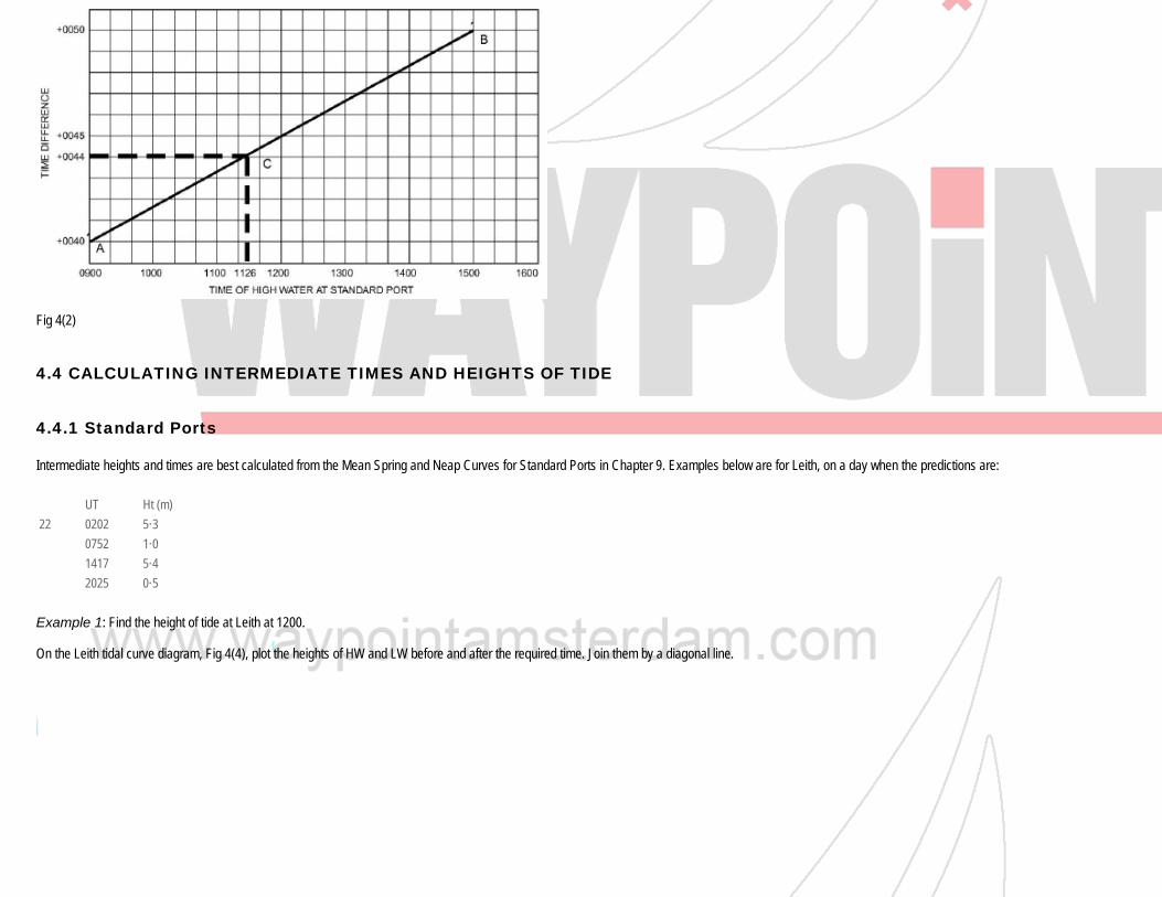
Fig 4(2)

4.4 CALCULATING INTERMEDIATE TIMES AND HEIGHTS OF TIDE

4.4.1 Standard Ports

Intermediate heights and times are best calculated from the Mean Spring and Neap Curves for Standard Ports in Chapter 9. Examples below are for Leith, on a day when the predictions are:

UT Ht (m)22 0202 5·3 0752 1·0 1417 5·4 2025 0·5

Example 1: Find the height of tide at Leith at 1200. On the Leith tidal curve diagram, Fig 4(4), plot the heights of HW and LW before and after the required time. Join them by a diagonal line.

Fig 4(3)

● Enter the HW time and other times as necessary in the boxes below the curves.● From the required time, go vertically to the curves. The Spring curve is red, and the Neap curve (where it differs) is blue. Interpolate between the curves by comparing the actual range, in this example 4·4m,

with the Mean Ranges printed beside the curves. Never extrapolate. Here the Spring curve applies.● Go horizontally to the diagonal line first plotted, thence vertically to the height scale, to extract 4·2m.

Fig 4(4) Curve for example 1

Example 2: Find the time in the afternoon when the height of tide has fallen to 3·7m.

● On Fig 4(5) plot the heights of HW and LW above and below the required height of tide. Join them by a sloping line.● In the boxes below the curves enter HW time and other hourly times to cover the required timescale.● From the required height, drop vertically to the diagonal line and thence horizontally to the curves. Interpolate between them as in Example 1; do not extrapolate. In this example the actual range is 4·9m, so

the Spring curve applies.● Drop vertically to the time scale, and read off the time required: 1637.

Fig 4(5) Curve for example 2

4.4.2 Secondary Ports

On coasts where the tidal curves for adjacent Standard Ports change little in shape, and where the duration of rise or fall at the Secondary Port is similar to its relevant Standard Port (ie where HW and LW time differences are nearly the same), intermediate times and heights are calculated from the tidal curves for the Standard Port in a similar manner to 4.4.1. The curves are entered with the times and heights of HW and LW at the Secondary Port, calculated as in 4.3.2 and 4.3.3. Interpolate by eye between the curves, using the range at the Standard Port as argument. Do not extrapolate – use the Spring curve for ranges greater than Springs, and the Neap curve for ranges less than Neaps. With a large change in duration between Springs and Neaps the results may have a slight error, greater near LW. For places between Christchurch and Selsey Bill (where the tidal regime is complex) special curves are given in 9.2.9.

4.4.3 The use of factors

Factors (in green on tidal curves) are another method of tidal calculation, but the Admiralty tidal prediction form (see 9.2.9) no longer contains the relevant fields. A factor of 1 = HW, and 0 = LW. Tidal curve diagrams show the factor of the range attained at times before and after HW. Thus the factor represents the percentage of the mean range (for the day in question) which has been reached at any particular time. Simple equations used are: Range x Factor = Rise or Factor = Rise ÷ Range

In determining or using the factor it may be necessary to interpolate between the Spring and Neap curves as described in 4.4.2. Factors are particularly useful when calculating hourly height predictions for ports with special tidal problems (9.2.9).

4.4.4 The Rule of Twelfths

The Rule of Twelfths estimates by mental arithmetic the height of the tide between HW and LW. It assumes that the duration of rise or fall is 6 hours, the curve is symmetrical and approximates to a sine curve. Thus the rule is invalid in the Solent, for example, where these conditions do not apply, nor should it be used if accuracy is critical.

The rule states that from one LW to the next HW, and vice versa, the tide rises or falls by: 1/12th of its range in the 1st hour 2/12ths of its range in the 2nd hour 3/12ths of its range in the 3rd hour 3/12ths of its range in the 4th hour 2/12ths of its range in the 5th hour 1/12th of its range in the 6th hour

4.4.5 Co-Tidal and Co-Range charts

5057 Dungeness to Hoek van Holland5058 British Isles and adjacent waters5059 Southern North Sea

These charts are used to predict tidal times and heights for an offshore position, as distinct from port or coastal locations which are covered by tide tables. There are Admiralty charts for the following offshore areas of NW Europe: They depict Co-Range and Co-Tidal lines, as defined below, with detailed instructions for use. A Co-Range line joins points of equal Mean Sp (or Np) Range which are simply the difference in level between MHWS and MLWS (or MHWN and MLWN). A Co-Tidal line joins points of equal Mean HW (or LW) Time Interval. This is defined as the mean time interval between the passage of the Moon over the Greenwich Meridian and the time of the next HW (or LW) at the place concerned. To find times and heights of tide at an offshore location, say in the Thames Estuary, needs some pre-planning especially if intending to navigate through a shallow gap. The Tidal Stream Atlas for the Thames Estuary (NP 249) also contains Co-Tidal and Co-Range charts. These are more clearly arranged and described than charts 5057–5059, but prior study is still necessary. The calculations require predictions for Sheerness, Walton-on-the-Naze or Margate, as relevant to the vessel’s position.

4.5 CALCULATING CLEARANCES BELOW OVERHEAD OBJECTS

A diagram often helps when calculating vertical clearances below bridges, power cables etc. Fig 4(6) shows the relationship to CD. The height of such objects as shown on the chart is usually measured above HAT, so the actual clearance will almost always be more. The height of HAT above CD is given at the foot of each page of the tide tables. Most Admiralty charts now show clearances above HAT, but check the Heights block below the chart Title.

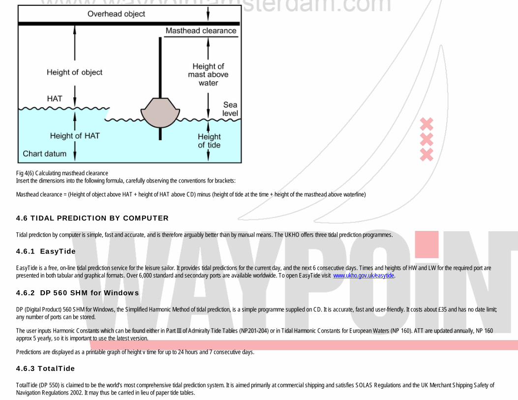
Fig 4(6) Calculating masthead clearance Insert the dimensions into the following formula, carefully observing the conventions for brackets: Masthead clearance = (Height of object above HAT + height of HAT above CD) minus (height of tide at the time + height of the masthead above waterline)

4.6 TIDAL PREDICTION BY COMPUTER

Tidal prediction by computer is simple, fast and accurate, and is therefore arguably better than by manual means. The UKHO offers three tidal prediction programmes.

4.6.1 EasyTide

EasyTide is a free, on-line tidal prediction service for the leisure sailor. It provides tidal predictions for the current day, and the next 6 consecutive days. Times and heights of HW and LW for the required port are presented in both tabular and graphical formats. Over 6,000 standard and secondary ports are available worldwide. To open EasyTide visit www.ukho.gov.uk/easytide.

4.6.2 DP 560 SHM for Windows

DP (Digital Product) 560 SHM for Windows, the Simplified Harmonic Method of tidal prediction, is a simple programme supplied on CD. It is accurate, fast and user-friendly. It costs about £35 and has no date limit; any number of ports can be stored. The user inputs Harmonic Constants which can be found either in Part III of Admiralty Tide Tables (NP201-204) or in Tidal Harmonic Constants for European Waters (NP 160). ATT are updated annually, NP 160 approx 5 yearly, so it is important to use the latest version. Predictions are displayed as a printable graph of height v time for up to 24 hours and 7 consecutive days.

4.6.3 TotalTide

TotalTide (DP 550) is claimed to be the world’s most comprehensive tidal prediction system. It is aimed primarily at commercial shipping and satisfies SOLAS Regulations and the UK Merchant Shipping Safety of Navigation Regulations 2002. It may thus be carried in lieu of paper tide tables.

TotalTide gives fast and accurate tidal predictions for over 7,000 ports and tidal stream data for more than 3,000 locations worldwide. The CD contains a free calculation programme. There are 10 Area Data Sets (ADS), with world-wide coverage costing about £400. However, each ADS can be bought for about £60. Areas 1-4 (see below) are in one ADS. Access is via a permit system. Annual updates are available, and are essential to satisfy safety regulations, although TotalTide will still run without them but less accurately. The ten ADS cover:

1–4. Europe, Mediterranean and northern waters5. Red Sea, the Gulf and Indian Ocean (north)6. Singapore to Japan and Philippines7. Australia and Borneo8. Pacific Ocean, New Zealand and America (west)9. North America (east coast) and Caribbean10. South Atlantic and Indian Ocean (southern part)

TotalTide displays 7 days of times and heights of HW and LW in both tabular and graphical formats. Other useful facilities include: a display of heights at specified times and time intervals; a continuous plot of height against time; indications of periods of daylight and twilight, moon phases, springs/neaps; the option to insert the yacht’s draft; calculations of under-keel and overhead clearances. TotalTide will run on most versions of Microsoft Windows, but check your system is compatible before buying.

4.6.4 Commercial software

Various commercial firms sell tidal prediction software for use on computers or calculators. Such software is mostly based on NP 159 and can often predict many years ahead. It remains essential to install annual updates.

4.7 TIDAL STREAMS

Tidal streams are the horizontal movement of water caused by the vertical rise and fall of the tide; see Fig 4(8). They normally change direction about every six hours. They are quite different from ocean currents, such as the Gulf Stream, which run indefinitely in the same direction. The direction (set) of a tidal stream is always that towards which it is running. The speed (rate) of tidal streams is important to yachtsmen: about 2kn is common, 6–8kn is not unusual in some areas at springs; 16kn has been recorded in the Pentland Firth.

4.7.1 Tidal stream atlases

Admiralty Tidal Stream Atlases, listed below, show the rate and set of tidal streams in the more important areas around the UK and NW Europe. The set is shown by arrows graded in weight and, where possible, in length to indicate the rate. The figures against the arrows give the mean Np and Sp rates in tenths of a knot; thus 19,34 indicates a mean Np rate of 1·9kn and a mean Sp rate of 3·4kn. The comma between 19 and 34 is roughly where the observations were made. Inshore eddies are rarely shown in detail due to limitations of scale. Tidal stream chartlets in this Almanac are derived from the following Admiralty Tidal Stream Atlases. NP Title

209 Orkney and Shetland Islands218 North Coast of Ireland, West Coast of Scotland

219 Portsmouth Harbour and Approaches220 Rosyth Harbour and Approaches221 Plymouth Harbour and Approaches222 Firth of Clyde and Approaches233 Dover Strait249 Thames Estuary (with co-tidal charts)250 The English Channel251 North Sea, Southern Part252 North Sea, North Western Part253 North Sea, Eastern Part254 The West Country, Falmouth to Teignmouth255 Falmouth to Padstow, including the Isles of Scilly256 Irish Sea and Bristol Channel257 Approaches to Portland258 Bristol Channel (Lundy to Avonmouth)259 Irish Sea, Eastern part263 Lyme Bay264 The Channel Islands and adjacent Coast of France265 France, West Coast337 The Solent and adjacent waters

Useful information is also given in Admiralty Sailing Directions: times of slack water, when the tide turns, overfalls, races etc. Along open coasts the tidal stream does not necessarily turn at HW and LW; it often occurs at about half tide. The tidal stream usually turns earlier inshore than offshore. In larger bays the tide often sets inshore towards the coast. The Yachtsman’s Manual of Tides by Michael Reeve-Fowkes (ACN) covers all theoretical and practical aspects of tides. It includes four regional Tidal Atlases: Western Channel; Central Channel and the Solent; Southern North Sea and Eastern Channel; Channel ports and approaches. These are also available separately. The atlases are referenced to HW Cherbourg and include annual Cherbourg tide tables (which are downloadable free from www.adlardcoles.com ).

4.7.2 Tidal stream diamonds

Lettered diamonds on many medium scale charts refer to tables on the chart giving the most accurate tidal stream set and rate (for springs and neaps) at hourly intervals before and after HW at a convenient Standard Port. See Fig 4(7).

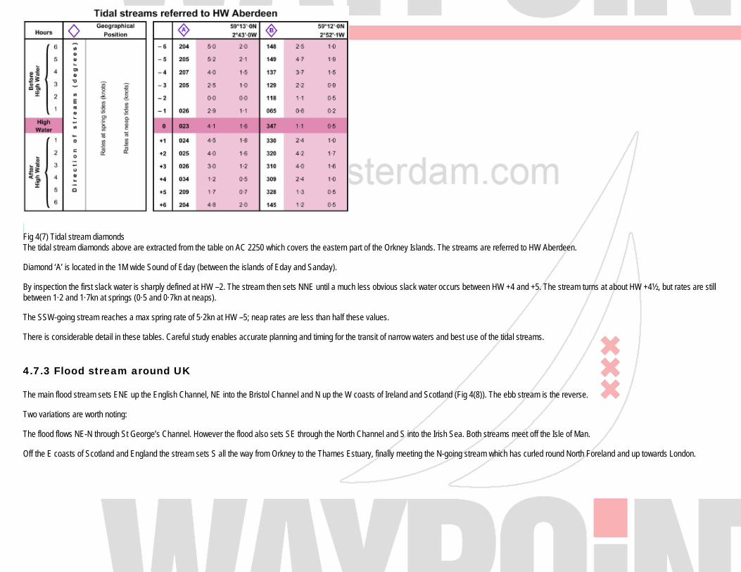
Fig 4(7) Tidal stream diamonds The tidal stream diamonds above are extracted from the table on AC 2250 which covers the eastern part of the Orkney Islands. The streams are referred to HW Aberdeen. Diamond ‘A’ is located in the 1M wide Sound of Eday (between the islands of Eday and Sanday). By inspection the first slack water is sharply defined at HW –2. The stream then sets NNE until a much less obvious slack water occurs between HW +4 and +5. The stream turns at about HW +4½, but rates are still between 1·2 and 1·7kn at springs (0·5 and 0·7kn at neaps). The SSW-going stream reaches a max spring rate of 5·2kn at HW –5; neap rates are less than half these values. There is considerable detail in these tables. Careful study enables accurate planning and timing for the transit of narrow waters and best use of the tidal streams.

4.7.3 Flood stream around UK

The main flood stream sets ENE up the English Channel, NE into the Bristol Channel and N up the W coasts of Ireland and Scotland (Fig 4(8)). The ebb stream is the reverse. Two variations are worth noting: The flood flows NE-N through St George’s Channel. However the flood also sets SE through the North Channel and S into the Irish Sea. Both streams meet off the Isle of Man. Off the E coasts of Scotland and England the stream sets S all the way from Orkney to the Thames Estuary, finally meeting the N-going stream which has curled round North Foreland and up towards London.

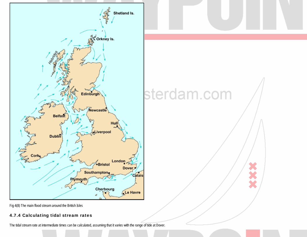
Fig 4(8) The main flood stream around the British Isles

4.7.4 Calculating tidal stream rates

The tidal stream rate at intermediate times can be calculated, assuming that it varies with the range of tide at Dover.

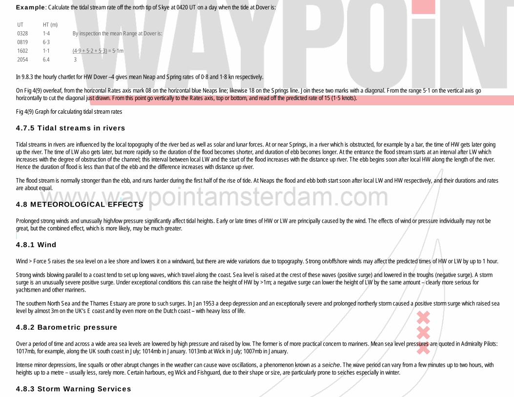
Example: Calculate the tidal stream rate off the north tip of Skye at 0420 UT on a day when the tide at Dover is:

UT HT (m) 0328 1·4 By inspection the mean Range at Dover is:0819 6·31602 1·1 (4·9 + 5·2 + 5·3) = 5·1m2054 6.4 3

In 9.8.3 the hourly chartlet for HW Dover –4 gives mean Neap and Spring rates of 0·8 and 1·8 kn respectively. On Fig 4(9) overleaf, from the horizontal Rates axis mark 08 on the horizontal blue Neaps line; likewise 18 on the Springs line. Join these two marks with a diagonal. From the range 5·1 on the vertical axis go horizontally to cut the diagonal just drawn. From this point go vertically to the Rates axis, top or bottom, and read off the predicted rate of 15 (1·5 knots). Fig 4(9) Graph for calculating tidal stream rates

4.7.5 Tidal streams in rivers

Tidal streams in rivers are influenced by the local topography of the river bed as well as solar and lunar forces. At or near Springs, in a river which is obstructed, for example by a bar, the time of HW gets later going up the river. The time of LW also gets later, but more rapidly so the duration of the flood becomes shorter, and duration of ebb becomes longer. At the entrance the flood stream starts at an interval after LW which increases with the degree of obstruction of the channel; this interval between local LW and the start of the flood increases with the distance up river. The ebb begins soon after local HW along the length of the river. Hence the duration of flood is less than that of the ebb and the difference increases with distance up river. The flood stream is normally stronger than the ebb, and runs harder during the first half of the rise of tide. At Neaps the flood and ebb both start soon after local LW and HW respectively, and their durations and rates are about equal.

4.8 METEOROLOGICAL EFFECTS

Prolonged strong winds and unusually high/low pressure significantly affect tidal heights. Early or late times of HW or LW are principally caused by the wind. The effects of wind or pressure individually may not be great, but the combined effect, which is more likely, may be much greater.

4.8.1 Wind

Wind > Force 5 raises the sea level on a lee shore and lowers it on a windward, but there are wide variations due to topography. Strong on/offshore winds may affect the predicted times of HW or LW by up to 1 hour. Strong winds blowing parallel to a coast tend to set up long waves, which travel along the coast. Sea level is raised at the crest of these waves (positive surge) and lowered in the troughs (negative surge). A storm surge is an unusually severe positive surge. Under exceptional conditions this can raise the height of HW by >1m; a negative surge can lower the height of LW by the same amount – clearly more serious for yachtsmen and other mariners. The southern North Sea and the Thames Estuary are prone to such surges. In Jan 1953 a deep depression and an exceptionally severe and prolonged northerly storm caused a positive storm surge which raised sea level by almost 3m on the UK’s E coast and by even more on the Dutch coast – with heavy loss of life.

4.8.2 Barometric pressure

Over a period of time and across a wide area sea levels are lowered by high pressure and raised by low. The former is of more practical concern to mariners. Mean sea level pressures are quoted in Admiralty Pilots: 1017mb, for example, along the UK south coast in July; 1014mb in January. 1013mb at Wick in July; 1007mb in January. Intense minor depressions, line squalls or other abrupt changes in the weather can cause wave oscillations, a phenomenon known as a seiche. The wave period can vary from a few minutes up to two hours, with heights up to a metre – usually less, rarely more. Certain harbours, eg Wick and Fishguard, due to their shape or size, are particularly prone to seiches especially in winter.

4.8.3 Storm Warning Services

These warn of possible coastal flooding caused by abnormal meteorological conditions. A negative storm surge causes abnormally low tidal levels in the Dover Strait, Thames Estuary and Southern North Sea. 6–12 hrs warning is given, Sept–April, when tidal levels at Dover, Sheerness or Lowestoft are forecast to be >1m below predicted levels. Warnings are broadcast by Navtex, HM Coastguard and the Channel Navigation Information Service (CNIS) on VHF and MF as normally used for navigation warnings.