4.14 FINDING THE TRUE TEMPERATURE OF THE OCEAN SURFACE

Elizabeth C. Kent*Southampton Oceanography Centre, Southampton UK.

Alexey KaplanLamont-Doherty Earth Observatory of Columbia University, Palisades, NY, USA.

and Peter K. TaylorSouthampton Oceanography Centre, Southampton UK.

1.. INTRODUCTION

Observations of Sea Surface Temperature (SST)made by merchant ships have been analysed toidentify random errors and biases which depend onhow the measurement was made.

Routine meteorological reports from merchant shipsare collated in the International - ComprehensiveOcean-Atmosphere Dataset (I-COADS, Woodruff etal. 1998). We have analysed reports from 1970 to1997 using metadata from the World MeteorologicalOrganisation “List of Selected, Supplementary andAuxiliary Ships” to give additional information on themethods of measurement for each ship report.

2. SST MEASUREMENT METHODS

The characteristics of the SST data will depend onhow the measurements were made. Most of the SSTmeasurements in the period 1970 to 1997 were madeusing either a bucket and thermometer or by reportingthe temperature of the engine intake cooling water. Asmaller number of reports were made using hullsensors which are thought to be more accurate. I-COADS contains a metadata flag giving the method ofmeasurements for some of the reports. Informationfrom the SST Indicator “SI” flag is plotted in Figure 1awhich shows that prior to 1981 only a subset of SSTreports from buckets can be positively identified.However we can also appeal to external metadatacontained in the World Meteorological Organisation(WMO) Report No. 47 the “List of Selected,Supplementary and Auxiliary Ships” which givesmethods of measurements for many of the ships.WMO Report No. 47 is available in annual files indigital form since 1973 and was published most yearsin paper form since 1954 (e.g. WMO 1994). Themethod of measurement can be associated withindividual reports using the ship callsign. Figure 1b

shows the combined information from both sources,the SI flag and WMO Report No. 47. Using all theavailable metadata gives a much larger subset of datafor analysis and allows the comparison of bucket andengine intake SST extending further back in time.

Year

Num

ber

of O

bser

vatio

ns p

er M

onth

Bucket

Engine Intake

Unidentified

Hull Sensor

Figure 1a: Number of ship reports by measurementtype identified from the COADS “SI”indicator between 1970 and 1997.

Bucket

Engine Intake

UnidentifiedHull Sensor

Year

Num

ber

of O

bser

vatio

ns p

er M

onth

Figure 1b: Number of ship reports by measurementtype identified from a combination of theCOADS “SI” indicator and WMO ReportNo. 47 between 1970 and 1997.

* Corresponding author address:Elizabeth Kent, James Rennell Division,Southampton Oceanography Centre, European Way,Southampton, SO14 3ZH, UK.email: eck@soc.soton.ac.uk

3. RANDOM ERRORS IN SST

The random errors in the dataset were estimatedusing a method based on that of Kent et al. (1999).They used the semivariogram method to separaterandom and spatial variability in a dataset of pairedship reports. Squared SST differences wereregressed against ship separation to give an estimateof variability at zero separation. We here adapt theirmethod by using a General Linear Model (GLM,McCullagh and Nelder, 1989) with a gamma functionerror distribution instead of a least-squaresregression. The gamma function has a longer tailthan the normal distribution (assumed when fittingwith least squares) and therefore better fits thedistribution of squared differences. Kent et al. (1999)found that their analysis was affected by a smallnumber of outliers: use of the GLM avoids thisproblem.

Figure 2 shows a time series of random errorestimates for all data (solid line) and also separatelyfor reports from buckets and engine intakes.Estimates were calculated for each 5° region for eachmonth where there was enough data. Theseestimates are then averaged to give a global errorestimate for each month. The most significantvariation is the difference in quality between engineintakes (dotted line) and bucket reports (dashed line).Engine intake reports typically contain nearly 50%more scatter than bucket SST reports. There ishowever some evidence that engine intake reportsare improving in quality, the average engine intakeSST error in the 1970s is 1.8°C, in the 1990s it hasdecreased to 1.5°C.

Figure 2: Random error estimates for SST (°C)calculated monthly for period 1970 to1997. Solid line (centre) is for all data,long-dashed line (bottom) for SST frombuckets and dotted line (top) for SST fromengine intakes. A 12-month running boxfilter has been applied to the monthlyestimates.

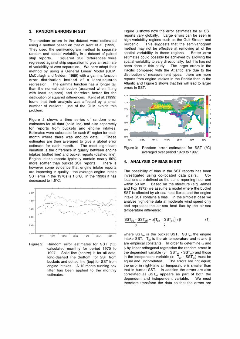
Figure 3 shows how the error estimates for all SSTreports vary globally. Large errors can be seen inhigh variability regions such as the Gulf Stream andKuroshio. This suggests that the semivariogrammethod may not be effective at removing all of thespatial variability in these regions. Better errorestimates could possibly be achieved by allowing thespatial variability to vary directionally, but this has notbeen done in this study. The larger errors in thePacific compared with the Atlantic are due to thedistribution of measurement types, there are morereports from engine intakes in the Pacific than in theAtlantic and Figure 2 shows that this will lead to largererrors in SST.

Figure 3: Random error estimates for SST (°C)averaged over period 1970 to 1997.

4. ANALYSIS OF BIAS IN SST

The possibility of bias in the SST reports has beeninvestigated using co-located data pairs. Co-locations are defined as the same reporting hour andwithin 50 km. Based on the literature (e.g. Jamesand Fox 1972) we assume a model where the bucketSST is affected by air-sea heat fluxes and the engineintake SST contains a bias. In the simplest case weanalyse night-time data at moderate wind speed onlyand represent the air-sea heat flux by the air-seatemperature difference:

SSTbu −SSTeriy

1 2 4 4 3 4 4 = α Tair −SSTeri( )

x1 2 4 4 3 4 4

+ β (1)

where SSTbu is the bucket SST, SSTeri the engineintake SST, Tair is the air temperature and α and βare empirical constants. In order to determine α andβ by linear orthogonal regression the random errors inthe dependent variable (y: SSTbu - SSTeri) and thosein the independent variable (x: Tair - SSTeri) must beequal and uncorrelated. The errors are not equal;the error in night-time air temperature is smaller thanthat in bucket SST. In addition the errors are alsocorrelated as SSTeri appears as part of both thedependent and independent variable. We musttherefore transform the data so that the errors are

equal and uncorrelated. This can be achieved bytransforming the data using an error correlationmatrix:

σair2 + σeri

2 σeri2

σeri2 σbu

2 + σeri2

(2)

where σair is the random error in the air temperaturemeasurement, σeri the random error in the engineintake SST and σbu is the random error in the bucketSST. The diagonal elements are the random error inx and y and the off-diagonal elements are thecorrelation between them which, in this simple case,is the random error in the engine intake SST. Theseerror estimates are those derived from semivariogramanalyses as described in Section 3. Once the datahave been transformed, a linear orthogonalregression can be performed and the resultingregression parameters transformed back to giveestimates for the model parameters α and β.

Results from a North Atlantic subset of January dataare shown in Figure 4. Figure 4a shows the bucketminus engine intake SST plotted against the air minussea temperature difference. The dashed line is theline of equality and data falling on or near this linecannot be distinguished from errors in the engineintake SST (which appears on both axes). Much ofthe data is contaminated by these errors as we knowthat the random error in engine intake SST is large(see Figure 2). The same data is shown in Figure 4bfollowing transformation using the error correlationmatrix. The errors in the transformed data shown inFigure 4b are equal and uncorrelated. An orthogonallinear regression has been performed and the upperand lower limits of the regression line are shown.The regression parameters are then transformed backinto the physical space and shown as the solid lines inFigure 4a. An estimate of the uncertainty in theregression has been made by repeating thecalculation with different values for the error estimates(equation 2). The elements of the covariance matrixwere adjusted to the limits of their error range to give

January Errors fall on this line

Regression line with error limits

Figure 4a: Bucket - engine intake SST plotted againstair-sea temperature difference. Dashedline indicates the contribution of errors inthe engine intake SST. Solid lines are theregression (from Figure 4b) and itsestimated uncertainty allowing for errorsand correlations in the data.

July

Figure 4c: As Figure 4a but for July.

Transformed data

Figure 4b: Data as in Figure 4a after transformationinto a data space where errors are equaland uncorrelated. The solid lines are therange of uncertainty in an orthogonal linearregression of the data.

Transformed data

Figure 4d: As Figure 4b but for July.

upper and lower limits for the regression estimate.The uncertainty in the regression itself was alsoincluded in the overall uncertainty estimate.

The regression estimate for January shown in Figure4a is well defined but this was not the case in July(Figure 4c) when there was a smaller range of air-seatemperature difference and little variation away fromthe dashed line. The transformed data (Figure 4d)shows much less structure than that for January andthe resulting regression uncertainty is large (Figure4c).

Figure 5 shows how the estimates of the regressionslope (α, the proportion of the air - sea temperaturedifference that appears as an error in the bucket SST)and intercept (β, the offset between the bucket andthe engine intake SST) vary with month. Outside thesummer months (June, July, August) α is 0.2 ± 0.1(Figure 5a). The estimate of β is not significantlydifferent from zero (Figure 5b)

-0.8

-0.6

-0.4

-0.2

0

0.2

0.4

Jan Feb Mar Apr May Jun Jul Aug Sep Oct Nov Dec

Figure 5a: Monthly variation of slope (α ): therelationship between Bucket SST errorand the air-sea temperature difference.

-0.5

-0.4

-0.3

-0.2

-0.1

0

0.1

0.2

0.3

0.4

0.5

Jan Feb Mar Apr May Jun Jul Aug Sep Oct Nov Dec

Figure 5b: Monthly variation of intercept (β): the offsetin the engine intake SST.

5. CONCLUSIONS

The results suggest that night-time bucket SST maybe biased cold. The magnitude of the bias varies withthe air-sea temperature difference. If we combine anaverage North Atlantic air-sea temperature differenceof 1.5°C with an fractional error (α) in the SST of 0.2,the bias, on average, is 0.3°C. This is similar to themean difference between bucket and engine intakeSST values found by previous studies. However, oncethe cold bias in the bucket SST is accounted for, themean offset between the bucket SST and engineintake SST is close to zero. This contradicts thosestudies which concluded that engine intake SST is,on average, biased warm due to heating of the waterby the ships engines. A supposition for which therewas no direct evidence.

This bias in the bucket-derived SST observations oforder a few tenths °C is climatologically significant;the magnitude of the effect will vary with time due totrends in the proportion of reports made by differentobserving methods.

Future work will involve extending the analysis to usemore complex models. For example wind speeddependence can be added, or the effect of the heatfluxes on the bucket SST studied. In order to extendthe analysis to daytime data the effect of solarradiation on the ship air temperatures needs first to beassessed and removed (Berry et al. 2003).

6. REFERENCES

Berry, D. I., E. C. Kent and P. K. Taylor, 2003:Improving Merchant Ship Air Temperatures usingan Analytical Model of Heating Errors, Extendedabstract in this volume.

James, R. W. and P. T. Fox, 1972: Comparative seasurface temperature measurements., Reports onMarine Science Affairs, No 5, (WMO336), 27 pp.

Kent, E. C., P. G. Challenor, and P. K. Taylor, 1999: AStatistical Determination of the RandomObservational Errors Present in VoluntaryObserving Ships Meteorological Reports. J AtmosOceanic Tech, 16, 905-914.

McCullagh, P. and Nelder J. A., 1989: Generallinearised models, Second Edition, Chapman andHall, 511 pp.

WMO, 1994: International List of Selected,Supplementary and Auxiliary Ships, WMO ReportNo. 47, WMO, Geneva, various pagination.

Woodruff, S. D., H. F. Diaz, J. D. Elms, and S. J.Worley, 1998: COADS Release 2 Data andMetadata Enhancements for Improvements ofMarine Surface Flux Fields. Physics andChemistry of the Earth, 23, 517-527.