41 FIXED HEAD SHORT TERM HYDRO THERMAL … HEAD... · The primary objective of the short term hydro thermal scheduling is to find the optimal amount of generated powers for hydro

International Journal of Electrical Engineering and Technology (IJEET), ISSN 0976 – 6545(Print),

ISSN 0976 – 6553(Online) Volume 3, Issue 2, July- September (2012), © IAEME

430

FIXED HEAD SHORT TERM HYDRO THERMAL GENERATION

SCHEDULING USING REAL VARIABLE GENETIC ALGORITHM

Deepika Yadav1, R. Naresh

2 and V. Sharma

3

Ph.D. Scholar, Professor, Associate Professor

Electrical Engineering Department,

National Institute of Technology Hamirpur, HP, India-177005 3Corresponding Author E-mail ID: [email protected]

2Email:[email protected],

[email protected]

ABSTRACT

The short term hydrothermal scheduling (STHTS) is a daily planning proposition in power system operation. The

main purpose of hydro thermal generation scheduling is to minimize the overall operation cost and to satisfy the

given constraints by scheduling optimally the power outputs of all hydro and thermal units under study periods,

given electrical load and limited water resource. This paper presents Real Variable Genetic Algorithm method for

fixed head hydro-thermal problem. Also, hydro power input-output model with constant head has been developed for

Sewa hydro electric power plant by using the curve fitting techniques namely least square method in MATLAB 7.9

version software. The control parameters of genetic algorithm have been optimized for the considered case study.

Keywords: Hydro-thermal scheduling, real-variable genetic algorithm, hydro power input-output model,

availability based tariff, valve-point loading

1. INTRODUCTION

Short-term hydrothermal scheduling is a crucial task in the economic operation of a power system. A good

generation schedule reduces the production cost, increases the system reliability, and maximises the energy

capability of reservoirs by utilizing the limited water resource. The primary objective of the short term hydro thermal

scheduling is to find the optimal amount of generated powers for hydro and thermal units so as to minimize the fuel

cost of thermal units. The problem requires that a given amount of water be used in such a way so as to achieve this

objective, which is usually much more complex than the scheduling of all thermal system. This is because if water

available is used up in the present interval there will not be any water for the next interval increasing this way the

future operation costs. Both electrically and hydraulically coupled hydro plants themselves are difficult to co-

ordinate with the thermal generation system to obtain minimum total system cost subject to various equality and

inequality constraints. The optimal scheduling of hydro thermal power system is basically a non-linear programming

problem involving non-linear objective function and a mixture of linear and non linear constraints.

No state or country is endowed with plenty of water sources or abundant coal and nuclear fuel. For minimum

environmental pollution and cost considerations, thermal generation should be minimum. Hence, a mix of hydro and

thermal-power generation is necessary. The states that have a large hydro-potential can supply excess hydro-power

during periods of high water run-off to other states and can receive thermal power during periods of low water run-

off from other states. The states, which have a low hydro-potential and large coal reserve, can use the small hydro-

power for meeting peak load requirements. This makes the thermal stations to operate at high load factors and to

have reduced installed capacity with the result economy. In states which have adequate hydro as well as thermal-

INTERNATIONAL JOURNAL OF ELECTRICAL ENGINEERING &

TECHNOLOGY (IJEET)

ISSN 0976 – 6545(Print)

ISSN 0976 – 6553(Online)

Volume 3, Issue 2, July – September (2012), pp. 430-443

© IAEME: www.iaeme.com/ijeet.html

Journal Impact Factor (2012): 3.2031 (Calculated by GISI)

www.jifactor.com

IJEET

© I A E M E



431

power generation capacities, power co-ordination to obtain a most economical operating state is essential. Maximum

advantage of cheap hydro-power should be taken so that the coal reserves can be conserved and environmental

pollution can be minimized. The whole or a part of the base load can be supplied by the run-off river hydro-plants,

and the peak or the remaining load is then met by a proper mix of reservoir type hydro-plants and thermal plants.

Determination of this by a proper mix is the determination of the most economical operating state of a hydro-thermal

system. The hydro-plants can be started easily and can be assigned a load in a very short time. However, in the case

of thermal plants, it requires several hours to make the boilers, super heater, and turbine system ready to take the

load. For this reason, the hydro-plants can handle fast-changing loads effectively. The thermal plants in contrast are

slow in response [1]. Hence, due to this, the thermal plants are more suitable to operate at base load plants, leaving

hydro-plants to operate at peak load plants. The operating cost of thermal plants is very high and at the same time its

capital cost is low when compared with a hydro-electric plant. The operating cost of a hydro-electric plant is low and

its capital cost is high such that it has become economical as well as convenient to run both thermal as well as hydro-

plants in the same grid.

Short-term hydro-thermal co-ordination, concerns with distributing the generation among the available units over a

day or week, usually on an hourly basis, satisfying the operational constraints, as well as reservoir release targets

determined by mid/ long-range planning models. In short-range scheduling problem, fixed water head is assumed

frequently and the net head variation can be ignored for relatively large reservoirs, in which case the power

generation is solely dependent on the water discharge [1 and 2]. Hydro thermal scheduling is a daily planning task in

power system operation and it is the subject of intensive investigation for several decades. Most of the methods that

have been used to solve the hydro thermal coordination problem make a number of simplifying assumption in order

to make the optimization problem more tractable.

Various conventional methods for solving the short term hydrothermal scheduling problems have been reported in

literature like Mixed integer linear programming [3], Dynamic programming [4], Lagrange relaxation method [5],

Interior point method [6] etc.

Based on the above review, it is observed that conventional/classical optimization methods suffer from

dimensionality difficulty, large memory requirement, large computation time, inability to handle nonlinear plus non-

separable objective function and constraints and unable to handle global optimum etc.

Recently, stochastic optimization techniques, such as genetic algorithms [7], simulated annealing [8], evolutionary

programming [9] and various other hybrid techniques [10] are also available for hydro thermal scheduling.

Here in this paper real variable genetic algorithm method for fixed head hydro thermal problem has been employed

and tested on a system of one hydro and three thermal systems. Also, model for hydro system is developed from the

experimental data set taken from Sewa hydro electric plant site of Jammu & Kashmir region.

This paper is structured as follows. Section 2 introduces modelling of hydro power input-output model. The short-

term hydro-thermal problem formulation is discussed in section 3. Section 4 presents overview of real coded genetic

algorithm. Section 5 and 6 describes algorithm and flow chart for hydro thermal scheduling. The test system results

of hydro thermal scheduling is presented in section 7 followed by conclusions.

2. HYDRO POWER INPUT-OUTPUT MODELLING

National Hydroelectric Power Corporation (NHPC) has encouraged various hydro electric projects in Himachal

Pradesh. One of them is Sewa hydro electric project stage-II (120MW), which is a run-off-the river project located in

kathua district of Jammu and Kashmir region. In this section hydro power input-output model for Sewa hydro electric

power plant has been presented. Electric power is a very important infrastructure of the overall development of a

nation. It is the tool to forge the economic growth of a country. The utilization of hydro-resources efficiently plays an

eminent role in the planning and operation of a power system where the hydro power generation plants contribute a

significant part of the total installed capacity. There has been, therefore, an ever increasing need for more and more

power generation recently in all the countries of the world. Running costs of the hydropower installation are very low

as compared to the thermal stations or the nuclear power stations and the hydraulic turbines can be put off and on in

matter of minutes.

Modelling of the hydro electric plant is a very complex task and as such there is no uniform modelling as each one is

unique to its location and requirement. The diversity of these designs makes it necessary to model each one

individually. The parameters of modelling are nonlinear and highly dependent on the control variables. Here hydro

electric generation is modelled at the plant level by aggregating the hydro units. The generated hydro power )P( H

depends on the specific weight of the water ( ψ ), on the flow rate (q) passing through the turbine in m3/s, on the net

head (h) on the turbine in meters (m) and on the efficiency of the plant, considering head loss in the pipeline and the

efficiency of the turbine and generator. Power generated by the power plant is presented below in (1), where the

numerical factor makes the appropriate unit conversions from (m) and (m3/s) to MW, taking into consideration both the

water density and the acceleration due to gravity [11].



432

1000

qhPH

ηψ= (1)

where,

HP =Available hydro power (MW)

η= Combined efficiency of turbine and generator set

ψ = Specific weight of water (N/m3), and is the product of density of water (kg/m3) and acceleration due to gravity

(m/s2)

q = Water flow through the turbine (Discharge) in (m3/sec)

h= Net head of water in meters (the difference in water level between upstream and downstream

of the turbine)

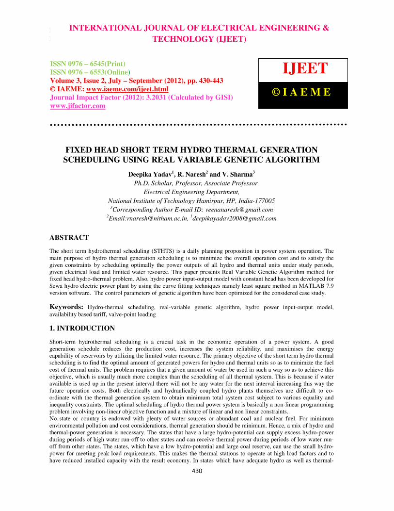
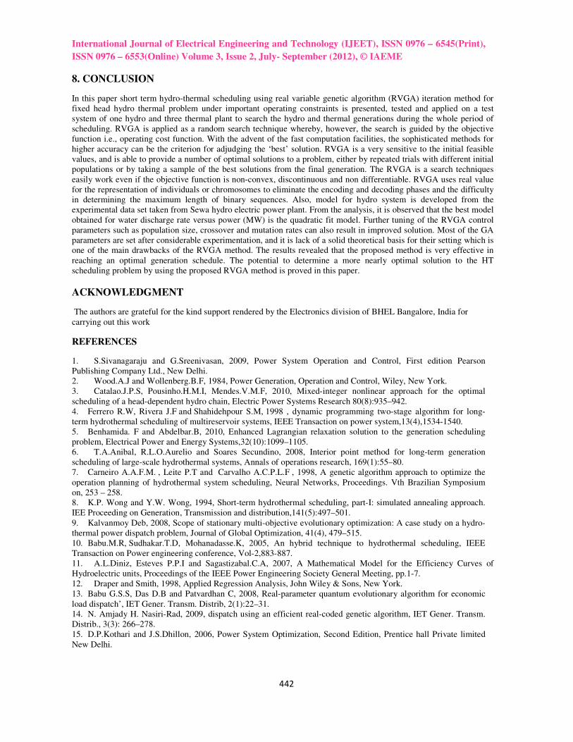
To model the input-output curve of the hydro power unit with constant head, experimental data has been obtained from

the site of Sewa hydro electric plant of Jammu and Kashmir region. The input is in terms of water discharge rate (

13sm −) whereas output is in terms of hydro power (MW).

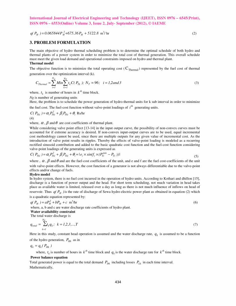
Figure1. Plot for actual and predicted results for water discharge rate versus power with constant

head

The relationship between water discharge rate and hydro power has been formed by using the curve fitting

techniques based on least square method [12]. As can be seen from figure 1, the second order quadratic equation (2)

very well satisfies the relation of generated power and water discharge rate as per data available from the site. The

thick dotted line, shown in figure 1, represents the actual relationship between the water discharge rate and hydro

power. Also, quadratic fit obtained from the experimental data is well within the 95% confidence interval.

International Journal of Electrical Engineering and Technology (IJEET), ISSN 0976

ISSN 0976 – 6553(Online) Volume 3, Issue 2, July

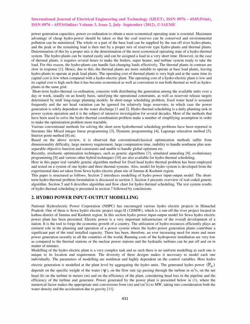
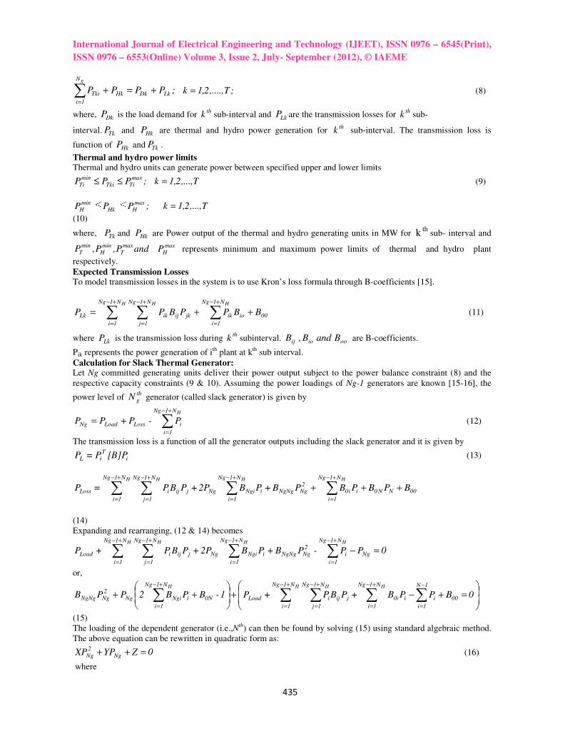
Figure 2. Residual plot for linear and quadratic regression models for water discharge rate versus

power (MW) with constant head

Figure 2 shows comparison of linear and quadratic models and it is found that the quadratic model gives better

performance with regard to magnitude of residuals at different points.

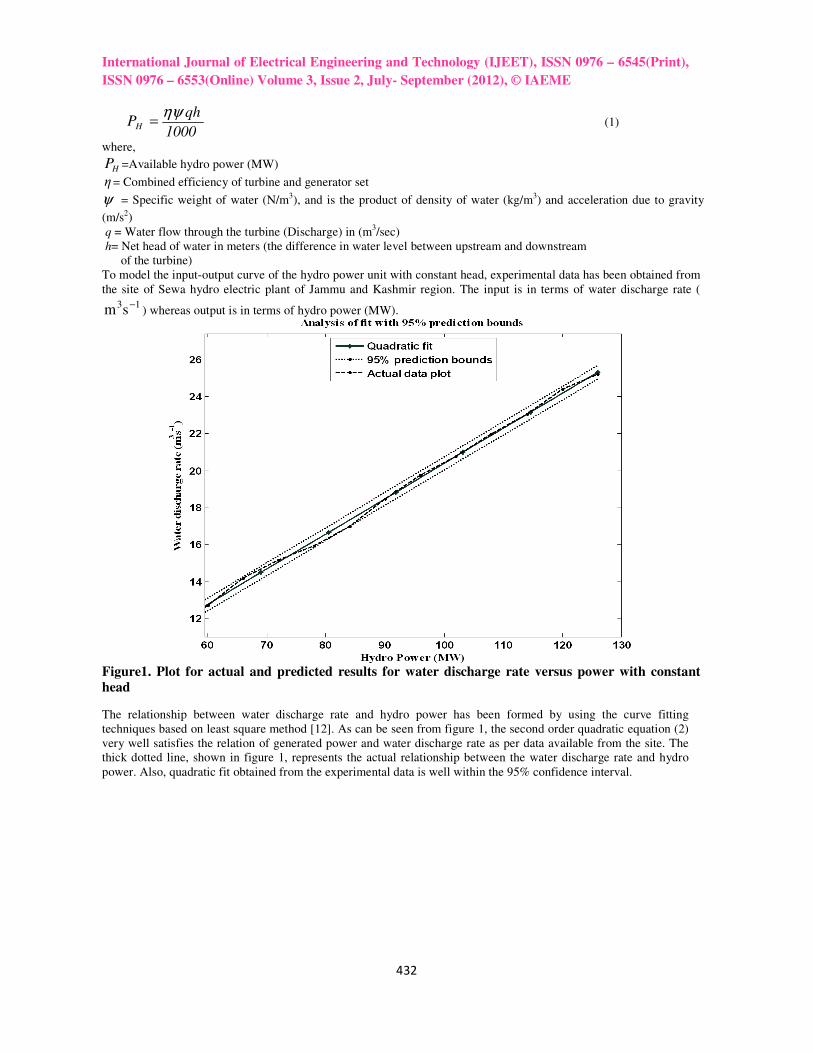
of square due to errors (SSE). For SSE a value closer to zero indicates that the model has small random error

component and that the corresponding fit will be useful for prediction.

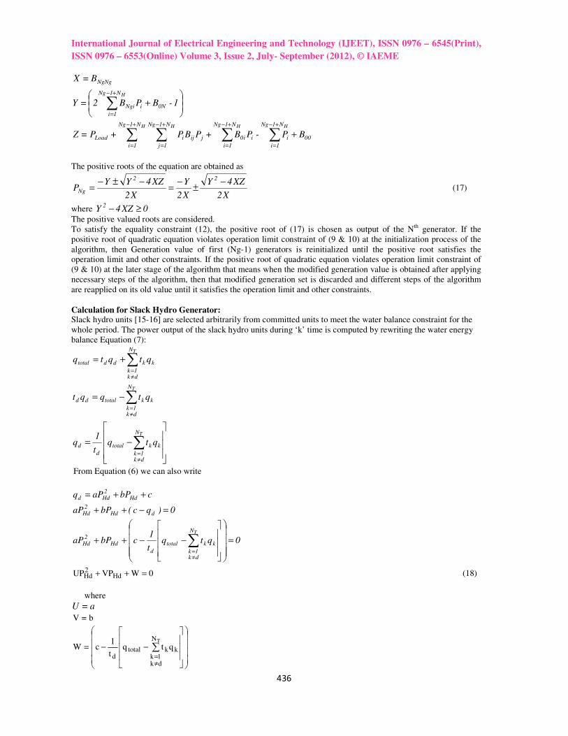
Figure 3. Plot for SSE and R

R-square values provide how well the model is close to actual values. In other words, it provides a measure of how

well future outcomes are likely to be predicted by the model. Hence it is desired that R

i.e., close to 1. As per the model 99% of variation in dep

From the graphical results the value of SSE is 0.4615 which was lowest in case of quadratic model and is within

acceptable limits. The input output model, which represents the ideal relationship b

)P( H and water discharge rate )q( for Sewa hydro electric project stage

International Journal of Electrical Engineering and Technology (IJEET), ISSN 0976

6553(Online) Volume 3, Issue 2, July- September (2012), © IAEME

433

2. Residual plot for linear and quadratic regression models for water discharge rate versus

shows comparison of linear and quadratic models and it is found that the quadratic model gives better

performance with regard to magnitude of residuals at different points. Figure 3, shows plot for R-square value, sum

are due to errors (SSE). For SSE a value closer to zero indicates that the model has small random error

component and that the corresponding fit will be useful for prediction.

Figure 3. Plot for SSE and R-square value

model is close to actual values. In other words, it provides a measure of how

well future outcomes are likely to be predicted by the model. Hence it is desired that R-square values to be very high

i.e., close to 1. As per the model 99% of variation in dependent variable has been explained by independent variable.


acceptable limits. The input output model, which represents the ideal relationship between generated hydro power

for Sewa hydro electric project stage-II, is


2. Residual plot for linear and quadratic regression models for water discharge rate versus

shows comparison of linear and quadratic models and it is found that the quadratic model gives better

square value, sum

are due to errors (SSE). For SSE a value closer to zero indicates that the model has small random error

model is close to actual values. In other words, it provides a measure of how

square values to be very high

endent variable has been explained by independent variable.


etween generated hydro power



434

8.5122P36.675P065844.0)P(q H2

HH ++= m3/ hr (2)

3. PROBLEM FORMULATION

The main objective of hydro thermal scheduling problem is to determine the optimal schedule of both hydro and

thermal plants of a power system in order to minimize the total cost of thermal generation. This overall schedule

must meet the given load demand and operational constraints imposed on hydro and thermal plant.

Thermal model

The objective function is to minimize the total operating cost ( ThermalC ) represented by the fuel cost of thermal

generation over the optimization interval (k).

);P(CtMinC Tk

N

1k

k

N

1i

Thermal

Tg

∑∑==

= ;96NT = 3and2,1i = (3)

where, kt is number of hours in th

k time block.

Ng is number of generating units

Here, the problem is to schedule the power generation of hydro-thermal units for k sub interval in order to minimize

the fuel cost. The fuel-cost function without valve-point loadings of th

i generating units.

iTkii2

TkiiTki PP)P(C θβα ++= Rs/hr

(4)

where, α , β andθ are cost coefficients of thermal plant.

While considering valve point effect [13-14] in the input output curve, the possibility of non-convex curves must be

accounted for if extreme accuracy is desired. If non-convex input-output curves are to be used, equal incremental

cost methodology cannot be used, since there are multiple outputs for any given value of incremental cost. As the

introduction of valve point results in ripples. Thereby the effects of valve-point loading is modeled as a recurring

rectified sinusoid contribution and added to the basic quadratic cost function and the fuel-cost function considering

valve-point loadings of the generating units is expressed as

|))P(Psin(fe|PP)P(C Timin

TiiiiTkii2

TkiiTki −××+++= θβα (5)

where , α , β andθ and are the fuel-cost coefficients of the unit, and e and f are the fuel cost-coefficients of the unit

with valve-point effects. However, the cost function of a generator is not always differentiable due to the valve-point

effects and/or change of fuels.

Hydro model

In hydro system, there is no fuel cost incurred in the operation of hydro units. According to Kothari and dhillon [15],

discharge is a function of power output and the head. For short term scheduling, not much variation in head takes

place as available water is limited, released over a day as long as there is not much influence of inflows on head of

reservoir. Thus )P(q H is the rate of discharge of Sewa hydro electric power plant as obtained in equation (2) which

is a quadratic equation represented by:

cbPaP)P(q H2

HH ++= m3/hr (6)

where, a, b and c are water discharge rate coefficients of hydro plant.

Water availability constraint The total water discharge is

;qtqTN

1k

kktotal ∑

=

= T,...,3,2,1k = (7)

Here in this study, constant head operation is assumed and the water discharge rate, kq is assumed to be a function

of the hydro generation, HkP as in

)P(qq Hkkk =

where, kt is number of hours in th

k time block and kq is the water discharge rate for th

k time block.

Power balance equation

Total generated power is equal to the total demand DkP including losses LkP in each time interval.

Mathematically,



435

;PPPP LkDkHk

N

1i

Tki

g

+=+∑=

;T,....,2,1k = (8)

where, DkP is the load demand for th

k sub-interval and LkP are the transmission losses for th

k sub-

interval. TkP and HkP are thermal and hydro power generation for th

k sub-interval. The transmission loss is

function of HkP and TkP .

Thermal and hydro power limits Thermal and hydro units can generate power between specified upper and lower limits

;PPPmax

TiTkimin

Ti ≤≤ T,...,2,1k = (9)

;PPP maxHHk

minH ≤≤ T,...,2,1k =

(10)

where, TkP and HkP are Power output of the thermal and hydro generating units in MW for th

k sub- interval and

andP,P,P maxT

minH

minT

maxHP represents minimum and maximum power limits of thermal and hydro plant

respectively.

Expected Transmission Losses To model transmission losses in the system is to use Kron’s loss formula through B-coefficients [15].

∑ ∑ ∑+−

=

+−

=

+−

=

++=H H HN1Ng

1i

N1Ng

1j

N1Ng

1i

00ioikjkijikLk BBPPBPP (11)

where LkP is the transmission loss during th

k subinterval. B and B ,B ooioij are B-coefficients.

Pik represents the power generation of ith

plant at kth

sub interval.

Calculation for Slack Thermal Generator: Let Ng committed generating units deliver their power output subject to the power balance constraint (8) and the

respective capacity constraints (9 & 10). Assuming the power loadings of Ng-1 generators are known [15-16], the

power level of thgN generator (called slack generator) is given by

∑+−

=

=HN1Ng

1i

iLossLoadNg P-P+PP (12)

The transmission loss is a function of all the generator outputs including the slack generator and it is given by

iT

iL [B]PP=P (13)

00NN0

N1Ng

1i

N1Ng

1j

i

N1Ng

1i

i02

NgNgNg

N1Ng

1i

iNgiNgjijiLoss BPBPBPB+PB2P+PBP=PH H HH

+++∑ ∑ ∑∑+−

=

+−

=

+−

=

+−

=

(14)

Expanding and rearranging, (12 & 14) becomes

0PP-PB+PB2P+PBP+P Ng

N1Ng

1i

i

N1Ng

1i

N1Ng

1j

2NgNgNg

N1Ng

1i

iNgiNgjijiLoad

HH H H

=−∑∑ ∑ ∑+−

=

+−

=

+−

=

+−

=

or,

=+−+

++ ∑ ∑∑ ∑∑

+−

=

−

=

+−

=

+−

=

+−

=

0BPPB+PBP+P1-BPB2PPBHH HH N1Ng

1i

1N

1i

00ii0i

N1Ng

1i

N1Ng

1j

jijiLoad0N

N1Ng

1i

iNgiNg2

NgNgNg

(15)

The loading of the dependent generator (i.e.,Nth

) can then be found by solving (15) using standard algebraic method.

The above equation can be rewritten in quadratic form as:

0ZYPXP Ng2

Ng =++ (16)

where



436

NgNgB =X

+∑

+−

=

1-BPB2 =Y 0N

N1Ng

1i

iNgi

H

00

N1Ng

1i

i

N1Ng

1i

N1Ng

1j

N1Ng

1i

ii0jijiLoad BP-PB+PBP+P=ZHH H H

+∑∑ ∑ ∑+−

=

+−

=

+−

=

+−

=

The positive roots of the equation are obtained as

X2

XZ4Y

X2

Y

X2

XZ4YYP

22

Ng

−±

−=

−±−= (17)

where 0XZ4Y2 ≥−

The positive valued roots are considered.

To satisfy the equality constraint (12), the positive root of (17) is chosen as output of the Nth

generator. If the

positive root of quadratic equation violates operation limit constraint of (9 & 10) at the initialization process of the

algorithm, then Generation value of first (Ng-1) generators is reinitialized until the positive root satisfies the

operation limit and other constraints. If the positive root of quadratic equation violates operation limit constraint of

(9 & 10) at the later stage of the algorithm that means when the modified generation value is obtained after applying

necessary steps of the algorithm, then that modified generation set is discarded and different steps of the algorithm

are reapplied on its old value until it satisfies the operation limit and other constraints.

Calculation for Slack Hydro Generator: Slack hydro units [15-16] are selected arbitrarily from committed units to meet the water balance constraint for the

whole period. The power output of the slack hydro units during ‘k’ time is computed by rewriting the water energy

balance Equation (7):

∑≠=

+=TN

dk1k

kkddtotal qtqtq

∑≠=

−=TN

dk1k

kktotaldd qtqqt

−= ∑≠=

TN

dk1k

kktotal

d

d qtqt

1q

From Equation (6) we can also write

cbPaPq Hd2

Hdd ++=

0)qc(bPaP dHd2

Hd =−++

0qtqt

1cbPaP

TN

dk1k

kktotal

d

Hd2

Hd =

−−++ ∑≠=

0WVPUP Hd2Hd =++ (18)

where

a =U

b=V

−− ∑

≠=

TN

dk1k

kktotald

qtqt

1c=W



437

The roots of the equation are obtained as

U2

UW4V

U2

V

U2

UW4VVP

22

Hd−

±−

=−±−

= (19)

where 0UW4V2 ≥−

The positive root is selected as a solution of (18). In this way power generation level of the hydro-generator during

slack time interval‘d’ is calculated.

4. REAL VARIABLE GENETIC ALGORITHM Real Variable Genetic Algorithm (RVGA) is a stochastic search algorithm [14] introduced by John Holland in

seventies as a special technique for function optimization [17]. It combines an artifice, i.e. the Darwinian Survival of

the Fittest principle with genetic operation, abstracted from nature to form a robust mechanism that is very effective

at finding optimal solutions to complex-real world problems. Genetic algorithms search for many points in the

search space at once, and continually narrow the focus of the search to the areas of the observed best performance.

The basic elements of real variable genetic algorithms are reproduction, crossover and mutation. In reproduction, the

individuals are selected based on their fitness values relative to those of the population. In the crossover operation,

two individual strings are selected at random from the mating pool and a crossover is performed using mathematical

relations. In mutation, an occasional random alteration of a member of population is done. Hereafter, we refer to it as

the classical GA (CGA). The performance of CGA precedes the traditional optimization methods in aspect of global

search and robustness in handling an arbitrary non-linear function. However, it suffers from premature convergence

problem and usually consumes enormous computing times.

In the CGA, ability of local search mainly relies on the reproduction and crossover operations, which can be referred

to as the exploitation operations, while the capability of global search is assured by the mutation operation, which

can be regarded as the exploration operation. Generally speaking, the velocity of local search increases when the

probability of crossover increases. Similarly, the level of capability of global search will increase when the

probability of mutation increases. Since the sum of probabilities of all the generic operations must be unity, in order

to assure a reasonable level of capability of local search, the mutation probability has to be reduced to increase the

crossover probability. This contributes to the fact that the probability of mutation in CGA is very low which usually

comes in a range of 0.1-5%. On the other hand, to achieve a satisfactory level of capability of global search, the

probabilities of reproduction and crossover have to be decreased to increase the mutation probability. This will

weaken capability of local search dramatically, slow down the convergence rate and makes the global search ability

unachievable eventually. In the process of balancing exploration and exploitation based on reproduction/crossover

and mutation operations for a fixed population, it is hardly possible to achieve the win-win situation for both sides

simultaneously. Therefore, how to balance between exploration and exploitation in GA-type algorithms has long

been a challenge task and retained its attractiveness to many researchers [18-19].

Every good GA needs to balance the extent of exploration of information obtained up until the current generation

through recombination and mutation operators with the extent of exploitation through the selection operator. If the

solutions obtained are exploited too much, premature convergence is expected. On the other hand, if too much stress

is given on a search (i.e. exploration), the information obtained thus far has not been used properly. Therefore, the

solution time may be enormous and the search exhibits a similar behaviour to that of a random search. The issue of

exploration and exploitation makes a recombination and mutation operator dependent on the chosen selection

operator for successful GA run. Majority of the improvements proposed were centralized in three aspects, i.e.,

decreasing the computing time, reducing premature convergence and enhancing global search capability. To reduce

computing time, some researchers proposed to use real-coded values instead of binary bit sequences [18-20]. Taking

this approach, the computation time spent on encoding/decoding has been eliminated, the diversity of mutation,

however, is significantly limited.

Two typical approaches are commonly used: one is to generate a new random value to replace the existing one and

the other is to add up one extra part, which is usually chosen randomly, to the existing one. None of them preserves

the meaning of natural mutation in a sense that the new value has nothing to do with the existing one. To enhance the

capability of global search, a lot of works have been done in increasing the diversity of the population [18-19].

4.1 Reproduction

The first genetic algorithm operator is reproduction. The reproduction genetic algorithm operator selects good

members in a population and forms a mating pool. The operator is also known as selection operator. The commonly

used reproduction operator is the proportionate reproduction operator where a string is selected for the mating pool

with a probability proportional to its fitness. The basic roulette wheel selection method is stochastic sampling with

replacement (SSR). The segment size and selection probability remain same throughout the selection phase and

individuals are selected accordingly. Stochastic sampling with partial replacement (SSPR) extends upon SSR by



438

resizing an individual’s segment if it is selected. Each time an individual is selected, the size of its segment is

reduced by one. If the segment size becomes negative, then it is set to zero. Remainder sampling methods involve

two distinct phases. In the integral phase, the individuals are selected deterministically according to the integer part

of their expected trials. The remaining individuals are then selected probabilistically from fractional part of the

individual’s expected values. The stochastic remainder roulette wheel selection is applied. This is the first of the

genetic operators. It is a process in which copies of the strings are copied into a separate string called the ‘mating

pool’, in proportion to their fitness values. This implies that strings with higher fitness values will have a higher

probability of contributing more strings as the search progresses. The present paper uses the roulette wheel method

[21] for the reproduction. In this method, each individual in the population is assigned a space on the roulette wheel,

which is proportional to the individual relative fitness. Individuals with the largest portion on the wheel have the

greatest probability to be selected as parent generation for the next generation.

4.2 Crossover Crossover is the main genetic operator and consists of swapping chromosome parts between individuals. Crossover

is not performed on every pair of individuals, its frequency being controlled by a crossover probability (PC). The

present paper uses arithmetic crossover operator. The basic concept of this operator is borrowed from the convex set

theory. Simple arithmetic operators are defined with the combination of two vectors (chromosomes) as follows:

)t()s)1((t

)t)1(()s(s

×+×−=′

×−+×=′

λλ

λλ

Where λ is uniformly distributed random variable between 0 and 1.

4.3 Mutation

After crossover, the strings are subjected to mutation. Mutation prevents the algorithm to be trapped in a local

minimum. Mutation plays the role of recovering the lost genetic materials as well as for randomly disturbing genetic

information. If crossover is supposed to exploit the current solution to find better ones, mutation is supposed to help

for the exploration of the whole search space. Mutation is viewed as a background operator to maintain genetic

diversity in the population. It introduces new genetic structures in the population by randomly modifying some of its

building blocks. Mutation helps escape from local minima’s trap and maintains diversity in the population [20]. Let

us suppose )C…,C…,(CC ni1= is a parent chromosome ]b,a[C iii ∈ is a gene to be mutated and ia and ib are

the lower and upper ranges for gene iC . A new gene in the offspring chromosomes, iC may arise from the

application of two different mutation operators respectively. The present paper uses uniform mutation operator. This

operator is single point random mutation, in which a single gene iC is randomly chosen number from range

]b,a[ ii to replace iC and to form new chromosome C' . It is controlled by mutation probability )(M c .Mutation is

done using following equation:

)C - rand(C+ C = C minjmax,jmin,jnew,

where,

Cmin,j and Cmax,j are the maximum and minimum value of jth variable.

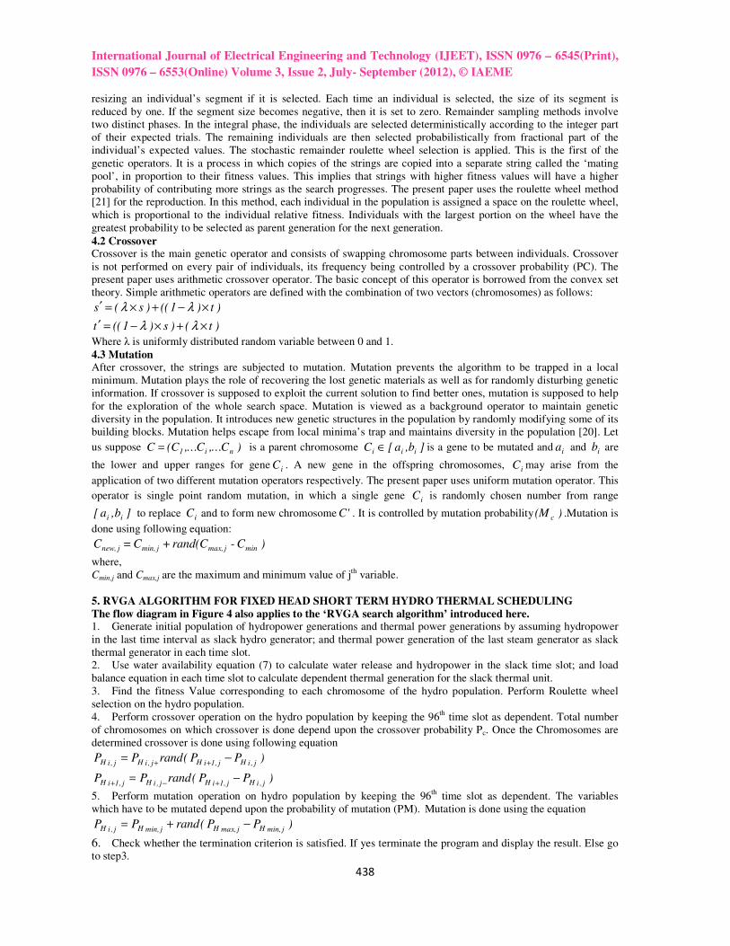
5. RVGA ALGORITHM FOR FIXED HEAD SHORT TERM HYDRO THERMAL SCHEDULING

The flow diagram in Figure 4 also applies to the ‘RVGA search algorithm’ introduced here. 1. Generate initial population of hydropower generations and thermal power generations by assuming hydropower

in the last time interval as slack hydro generator; and thermal power generation of the last steam generator as slack

thermal generator in each time slot.

2. Use water availability equation (7) to calculate water release and hydropower in the slack time slot; and load

balance equation in each time slot to calculate dependent thermal generation for the slack thermal unit.

3. Find the fitness Value corresponding to each chromosome of the hydro population. Perform Roulette wheel

selection on the hydro population.

4. Perform crossover operation on the hydro population by keeping the 96th

time slot as dependent. Total number

of chromosomes on which crossover is done depend upon the crossover probability Pc. Once the Chromosomes are

determined crossover is done using following equation

)PP(randPPj,iHj,1iHj,iHj,iH −=

++

)PP(randPPj,iHj,1iHj,iHj,1iH −=

+−+

5. Perform mutation operation on hydro population by keeping the 96th

time slot as dependent. The variables

which have to be mutated depend upon the probability of mutation (PM). Mutation is done using the equation

)PP(randPPjmin,Hjmax,Hjmin,Hj,iH −+=

6. Check whether the termination criterion is satisfied. If yes terminate the program and display the result. Else go

to step3.



439

6 .Flow chart for RVGA

Figure 4.Flowchart for RVGA



440

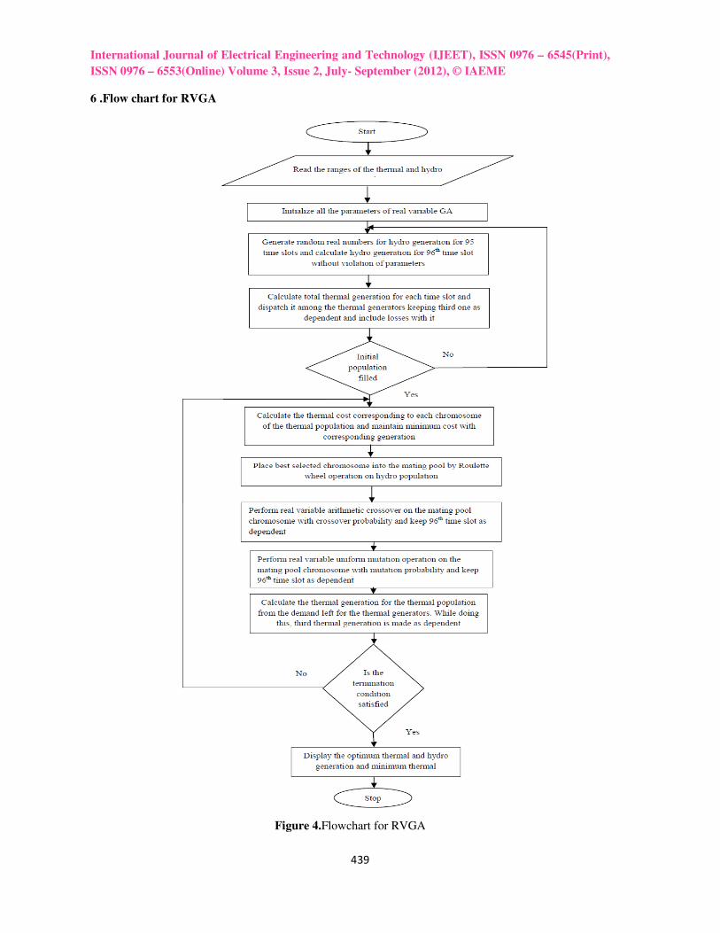
7. Test system

Normally, short term hydro thermal scheduling concerns with one day to week periods of operation with interval of

various lengths [1-2 and 15]. This paper focuses on short term hydro thermal scheduling (STHTS), in which day

ahead scheduling is done for 24 hours on 15 minutes time interval [22-23]. Total load demand over 24 hours period

for 96 time interval is shown in figure 5. The test system comprises of a Sewa hydro power plant and three thermal

units, that have been adopted from [24 and 15].The real variable genetic algorithm was implemented in MATLAB

7.9 and executed on a PC (Pentium-IV, 512MB, 3.0GHz). In both test cases 30 independent runs were conducted

with different random initial solution for each run. The polynomial cost coefficients of the hydro electric system

were estimated from experimental data of sewa hydro electric plant site by curve fitting technique. The equivalent

hydro system obtained with 9995.0R2 = and SSE=0.4615 is presented in section 2.1. The equivalent hydro system

obtained is 8.5122P36.675P065844.0)P(q H2

HH ++= m3/ hr. The lower and upper limits of hydro units for

Sewa hydro electric power plant are 12MW and 126MW respectively. The characteristic functions of three thermal

plants [24 and 15] considering valve point loading are defined as follows

|))P(50sin(0.0315200|100P1.0P01.0C 1T1T21T1 −××+++=

|))P(40sin(0.0420170|120P1.0P02.0C 2T2T22T2 −××+++=

|))P(30sin(0.0630215|150P1.0P01.0C 3T3T23T3 −××+++=

The boundary condition of the problem is defined by the upper and lower limits of the generation capacity of the

four plants that are given by:

MW200)t(PMW50 1T ≤≤

MW170)t(PMW40 2T ≤≤

MW215)t(PMW30 3T ≤≤

MW126)t(PMW12 1H ≤≤

The system electrical losses are associated with the hydro plant and three steam plants are expressed as follows:

=

0005.0000

000025.000

000005.00

00000004.0

B1MW −

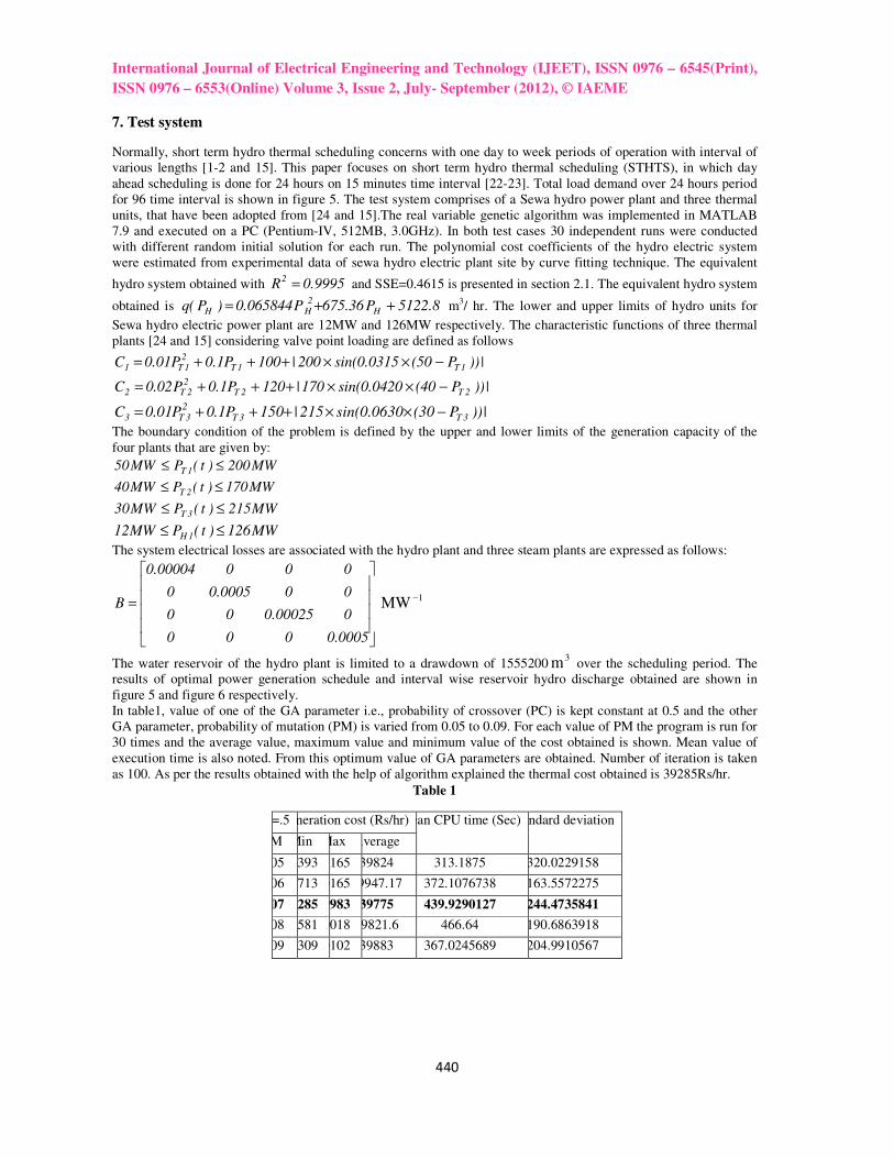
The water reservoir of the hydro plant is limited to a drawdown of 15552003m over the scheduling period. The

results of optimal power generation schedule and interval wise reservoir hydro discharge obtained are shown in

figure 5 and figure 6 respectively.

In table1, value of one of the GA parameter i.e., probability of crossover (PC) is kept constant at 0.5 and the other

GA parameter, probability of mutation (PM) is varied from 0.05 to 0.09. For each value of PM the program is run for

30 times and the average value, maximum value and minimum value of the cost obtained is shown. Mean value of

execution time is also noted. From this optimum value of GA parameters are obtained. Number of iteration is taken

as 100. As per the results obtained with the help of algorithm explained the thermal cost obtained is 39285Rs/hr.

Table 1

PC=.5 Generation cost (Rs/hr) Mean CPU time (Sec) Standard deviation

PM Min Max Average

0.05 39393 40165 39824 313.1875 320.0229158

0.06 39713 40165 39947.17 372.1076738 163.5572275

0.07 39285 39983 39775 439.9290127 244.4735841

0.08 39581 40018 39821.6 466.64 190.6863918

0.09 39309 40102 39883 367.0245689 204.9910567



441

Figure 5. Hourly hydro and thermal generation scheduling for a day

Figure 6. Hydro plant discharges ( hr/m10 34)

0 10 20 30 40 50 60 70 80 90 1000

100

200

300

400

500

600

700

Number of interval (96 time slot for 24 hours)

Dem

an

d a

nd

Gen

era

tio

n,

MW

Load Demand

Total Hydro Generation

TP1

PT2

PT3

0 10 20 30 40 50 60 70 80 90 1000

0.5

1

1.5

2

2.5

3x 10

4

Number of interval

Hy

dro

Dis

ch

arg

e



442

8. CONCLUSION

In this paper short term hydro-thermal scheduling using real variable genetic algorithm (RVGA) iteration method for

fixed head hydro thermal problem under important operating constraints is presented, tested and applied on a test

system of one hydro and three thermal plant to search the hydro and thermal generations during the whole period of

scheduling. RVGA is applied as a random search technique whereby, however, the search is guided by the objective

function i.e., operating cost function. With the advent of the fast computation facilities, the sophisticated methods for

higher accuracy can be the criterion for adjudging the ‘best’ solution. RVGA is a very sensitive to the initial feasible

values, and is able to provide a number of optimal solutions to a problem, either by repeated trials with different initial

populations or by taking a sample of the best solutions from the final generation. The RVGA is a search techniques

easily work even if the objective function is non-convex, discontinuous and non differentiable. RVGA uses real value

for the representation of individuals or chromosomes to eliminate the encoding and decoding phases and the difficulty

in determining the maximum length of binary sequences. Also, model for hydro system is developed from the

experimental data set taken from Sewa hydro electric power plant. From the analysis, it is observed that the best model

obtained for water discharge rate versus power (MW) is the quadratic fit model. Further tuning of the RVGA control

parameters such as population size, crossover and mutation rates can also result in improved solution. Most of the GA

parameters are set after considerable experimentation, and it is lack of a solid theoretical basis for their setting which is

one of the main drawbacks of the RVGA method. The results revealed that the proposed method is very effective in

reaching an optimal generation schedule. The potential to determine a more nearly optimal solution to the HT

scheduling problem by using the proposed RVGA method is proved in this paper.

ACKNOWLEDGMENT

The authors are grateful for the kind support rendered by the Electronics division of BHEL Bangalore, India for

carrying out this work

REFERENCES

1. S.Sivanagaraju and G.Sreenivasan, 2009, Power System Operation and Control, First edition Pearson

Publishing Company Ltd., New Delhi.

2. Wood.A.J and Wollenberg.B.F, 1984, Power Generation, Operation and Control, Wiley, New York.

3. Catalao.J.P.S, Pousinho.H.M.I, Mendes.V.M.F, 2010, Mixed-integer nonlinear approach for the optimal

scheduling of a head-dependent hydro chain, Electric Power Systems Research 80(8):935–942.

4. Ferrero R.W, Rivera J.F and Shahidehpour S.M, 1998 , dynamic programming two-stage algorithm for long-

term hydrothermal scheduling of multireservoir systems, IEEE Transaction on power system,13(4),1534-1540.

5. Benhamida. F and Abdelbar.B, 2010, Enhanced Lagrangian relaxation solution to the generation scheduling

problem, Electrical Power and Energy Systems,32(10):1099–1105.

6. T.A.Anibal, R.L.O.Aurelio and Soares Secundino, 2008, Interior point method for long-term generation

scheduling of large-scale hydrothermal systems, Annals of operations research, 169(1):55–80.

7. Carneiro A.A.F.M. , Leite P.T and Carvalho A.C.P.L.F , 1998, A genetic algorithm approach to optimize the

operation planning of hydrothermal system scheduling, Neural Networks, Proceedings. Vth Brazilian Symposium

on, 253 – 258.

8. K.P. Wong and Y.W. Wong, 1994, Short-term hydrothermal scheduling, part-I: simulated annealing approach.

IEE Proceeding on Generation, Transmission and distribution,141(5):497–501.

9. Kalvanmoy Deb, 2008, Scope of stationary multi-objective evolutionary optimization: A case study on a hydro-

thermal power dispatch problem, Journal of Global Optimization, 41(4), 479–515.

10. Babu.M.R, Sudhakar.T.D, Mohanadasse.K, 2005, An hybrid technique to hydrothermal scheduling, IEEE

Transaction on Power engineering conference, Vol-2,883-887.

11. A.L.Diniz, Esteves P.P.I and Sagastizabal.C.A, 2007, A Mathematical Model for the Efficiency Curves of

Hydroelectric units, Proceedings of the IEEE Power Engineering Society General Meeting, pp.1-7.

12. Draper and Smith, 1998, Applied Regression Analysis, John Wiley & Sons, New York.

13. Babu G.S.S, Das D.B and Patvardhan C, 2008, Real-parameter quantum evolutionary algorithm for economic

load dispatch’, IET Gener. Transm. Distrib, 2(1):22–31.

14. N. Amjady H. Nasiri-Rad, 2009, dispatch using an efficient real-coded genetic algorithm, IET Gener. Transm.

Distrib., 3(3): 266–278.

15. D.P.Kothari and J.S.Dhillon, 2006, Power System Optimization, Second Edition, Prentice hall Private limited

New Delhi.



443

16. Aniruddha Bhattacharya and Pranab Kumar Chattopadhyay, 2010, Hybrid Differential Evolution with

Biogeography-Based Optimization for Solution of Economic Load Dispatch, IEEE Transactions on Power Systems,

25(4):1955-1964.

17. J. H. Holland, 1975, Adaptation in Natural and Artificial Systems. Ann Arbor, MI: Univ. Michigan Press.

18. E. Alba, F. Luna and J M Troya, 2004, Parallel heterogeneous genetic algorithms for continuous optimization,

Parallel and nature-inspired computational paradigms and applications, 30(5-6):99-719.

19. S. Choi and C. Wu, 1998, Partitioning and allocation of objects in heterogeneous distributed environments using

the niched Pareto genetic-algorithm, in Proc. Asia Pacific Software Engineering Conference, pp. 322 – 329.

20. R. M. Ramos, R. R. Saldanha, R. H. C. Takahashi and F. J. S. Moreira, 2003 The real-biased multiobjective

genetic algorithm and its application to the design of wire antennas, IEEE Trans. Magn., Vol. 39, p. 1329-1332.

21. Genetic Algorithms in search, optimization & Machine learing by David E.Goldberg, Pearson Education, 1989.

22. Bhushan Bhanu, Roy Anjan and P.Pentayya, 2004 The Indian medicine, In IEEE Power Engineering Society

General Meeting, 2:2336 – 2339.

23. T.Geetha and V.Jayashankar, 2008 Generation Dispatch with Storage and Renewables under Availability Based

Tariff. In Proceedings of TENCON 2008, IEEE Region 10 Conference, pp.1-6.

24. Farhat, I.A and El-Hawary, M.E, 2010, Fixed-head hydro-thermal scheduling using a modified bacterial

foraging algorithm, IEEE Transaction on Electrical power and Energy conference, 1-6.

Documents

41 FIXED HEAD SHORT TERM HYDRO THERMAL … HEAD... · The primary objective of the short term hydro thermal scheduling is to find the optimal amount of generated powers for hydro