4.1 - 1 Copyright © 2010, 2007, 2004 Pearson Education, Inc. Section 4-2 Basic Concepts of Probability

4.1 - 1Copyright © 2010, 2007, 2004 Pearson Education, Inc.

Section 4-2 Basic Concepts of

Probability


Events and Sample Space

Event

any collection of results or outcomes of a procedure

Outcome (simple event)

It cannot be further broken down into simpler components

Sample Space

It consists of all possible outcomes that cannot be broken down any further


Notation for Probabilities

P - denotes a probability.

A, B, and C - denote specific events.

P(A) - denotes the probability of event A occurring.


Basic Rules for Computing Probability (1)

Rule 1: Probability by Relative Frequency

Conduct (or observe) a procedure, and count the number of times the event A actually occurs. Based on these actual results, P(A) is approximated as follows:

P(A) = # of times A occurred

# of times procedure was repeated



Rule 2: Exact Probability by Counting

(Requires Equally Likely Outcomes)

Assume that a given procedure has n different outcomes and that each of those outcomes has an equal chance of occurring. If event A can occur in s of these n ways, then

P(A) = # of outcomes in A

# of all the different outcomes



Rule 3: Subjective Probabilities

P(A), the probability of event A, is

estimated by using knowledge of the

relevant circumstances.


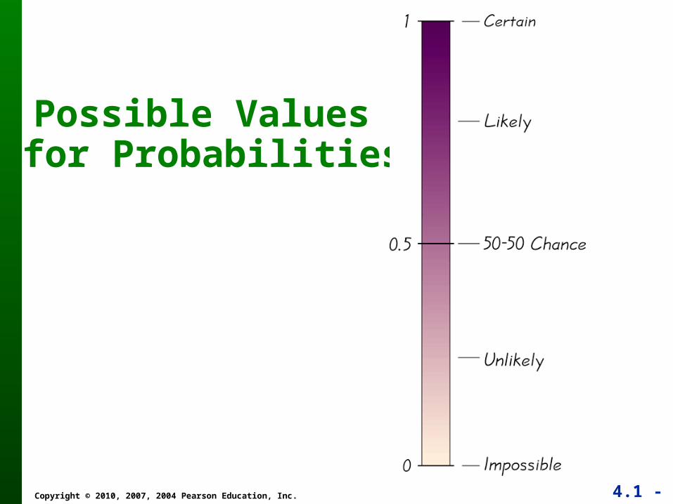
Possible Values for Probabilities


Rounding Off Probabilities

When expressing the value of a probability, either give the exact fraction or decimal or round off final decimal results to three significant digits. (Suggestion: When a probability is not a simple fraction such as 2/3 or 5/9, express it as a decimal so that the number can be better understood.)


Complementary Events

The complement of event A, denoted by

A

It consists of all outcomes in which the

event A does not occur.


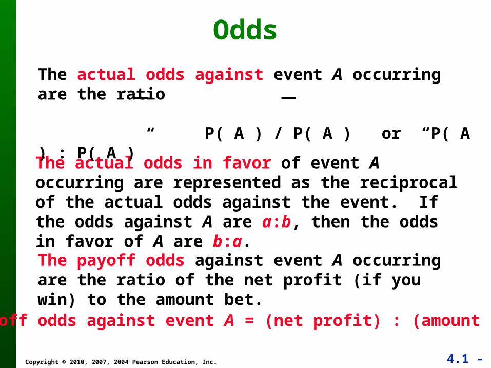
The actual odds in favor of event A occurring are represented as the reciprocal of the actual odds against the event. If the odds against A are a:b, then the odds in favor of A are b:a.

The actual odds against event A occurring are the ratio

P( A ) / P( A ) or “P( A ) : P( A )”

Odds

The payoff odds against event A occurring are the ratio of the net profit (if you win) to the amount bet.

payoff odds against event A = (net profit) : (amount bet)


Section 4-3 Addition Rule


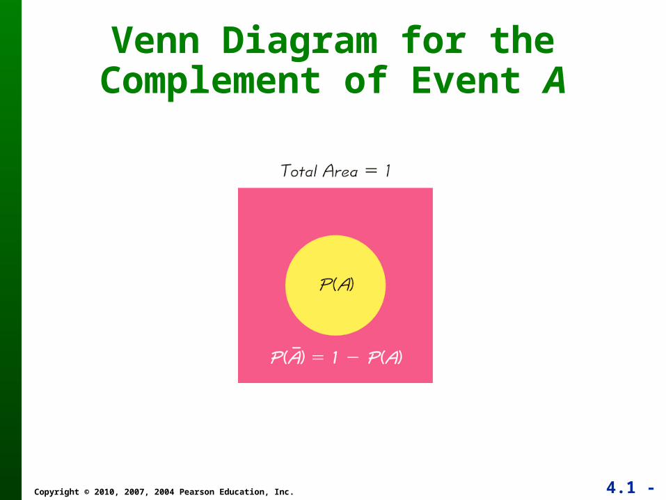
Complementary Events

P(A) and P(A )are disjoint

It is impossible for an event and its complement to occur at the same time.


Venn Diagram for the Complement of Event A


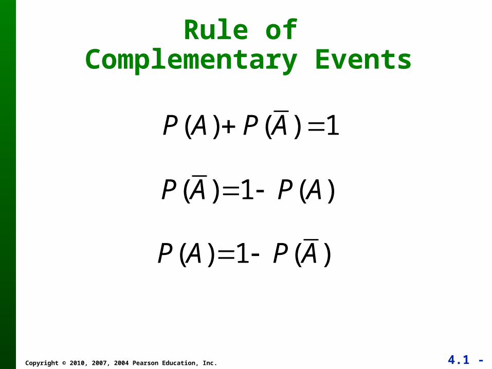
Rule of Complementary Events

( ) ( ) 1P A P A

( ) 1 ( )P A P A

( ) 1 ( )P A P A


Compound Event It represents any event combining 2 or more

outcomes (simple events)

Compound Event

Notation

P(A or B) = P (in a single trial, event A occurs or event B occurs or they both occur)


When finding the probability that event A occurs or event B occurs, we can find the total number of ways A can occur and the number of ways B can occur. However, the total number has to be counted in such a way that no outcome is counted more than once.

General Rule for a Compound Event


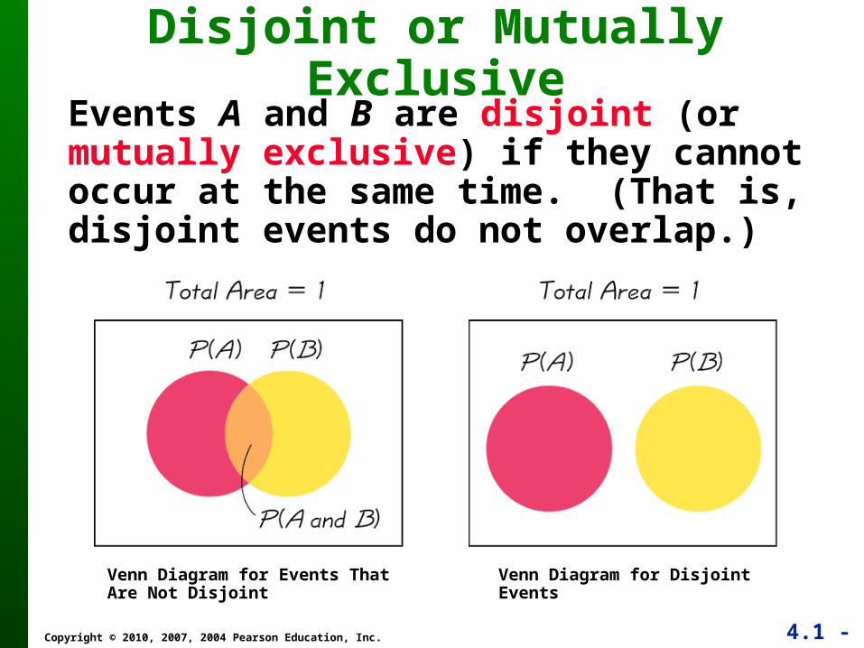
Disjoint or Mutually ExclusiveEvents A and B are disjoint (or mutually exclusive) if they cannot occur at the same time. (That is, disjoint events do not overlap.)

Venn Diagram for Events That Are Not Disjoint

Venn Diagram for Disjoint Events


Compound Event

Formal Addition Rule

P(A or B) = P(A) + P(B) – P(A and B)

where P(A and B) denotes the probability that A and B both occur at the same time as an outcome in a trial of a procedure.


Compound Event

Intuitive Addition Rule

To find P(A or B), find the sum of the number of ways event A can occur and the number of ways event B can occur, adding in such a way that every outcome is counted only once. P(A or B) is equal to that sum, divided by the total number of outcomes in the sample space.


Section 4-4 Multiplication Rule:

Basics


Notation

P(A and B) =

P(event A occurs in a first trial and

event B occurs in a second trial)


Intuitive Multiplication Rule

When finding the probability that event A occurs in one trial and event B occurs in the next trial, multiply the probability of event A by the probability of event B, but be sure that the probability of event B takes into account the previous occurrence of event A.


Dependent and Independent

Two events A and B are independent if the occurrence of one does not affect the probability of the occurrence of the other. (Several events are similarly independent if the occurrence of any does not affect the probabilities of the occurrence of the others.) If A and B are not independent, they are said to be dependent.


Conditional ProbabilityImportant Principle

The probability for the second event B should take into account the fact that the first event A has already occurred.


Notation for Conditional Probability

P(B|A) represents the probability of event B occurring after it is assumed that event A has already occurred (read B|A as “B given A.”)


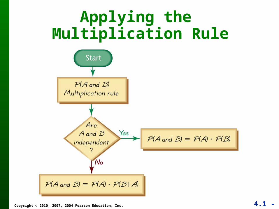
Applying the Multiplication Rule


Multiplication Rule for Several Events

In general, the probability of any sequence of independent events is simply the product of their corresponding probabilities.


Treating Dependent Events as Independent

Some calculations are cumbersome, but they can be made manageable by using the common practice of treating events as independent when small samples are drawn from large populations. In such cases, it is rare to select the same item twice.


The 5% Guideline for Cumbersome Calculations

If a sample size is no more than 5% of the size of the population, treat the selections as being independent (even if the selections are made without replacement, so they are technically dependent).


Section 4-5 Multiplication Rule:Complements and

Conditional Probability


Complements: The Probability of “At Least One”

The complement of getting at least one item of a particular type is that you get no items of that type.

“At least one” is equivalent to “one or more.”


Finding the Probability of “At Least One”

To find the probability of at least one of something, calculate the probability of none, then subtract that result from 1. That is,

P(at least one) = 1 – P(none).


Conditional ProbabilityA conditional probability of an event is a probability obtained with the additional information that some other event has already occurred. P(B|A) denotes the conditional probability of event B occurring, given that event A has already occurred, and it can be found by dividing the probability of events A and B both occurring by the probability of event A:

P(B|A) = P(A and B) / P(A)


Intuitive Approach to Conditional Probability

The conditional probability of B given A can be found by assuming that event A has occurred, and then calculating the probability that event B will occur.


Confusion of the Inverse

To incorrectly believe that P(A|B) and P(B|A) are the same, or to incorrectly use one value for the other, is often called confusion of the inverse.


Section 4-7Counting


Fundamental Counting Rule

For a sequence of two events in which the first event can occur m ways and the second event can occur n ways, the events together can occur a total of m n ways.


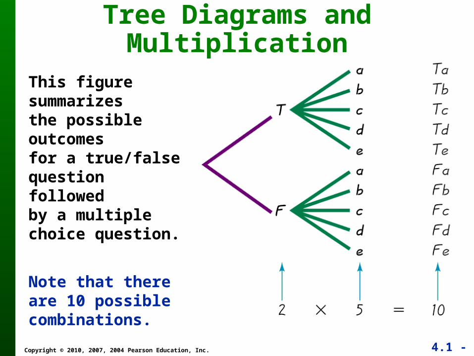
Tree Diagrams and Multiplication

This figure summarizes the possible outcomes for a true/false question followed by a multiple choice question.

Note that there are 10 possible combinations.


Notation

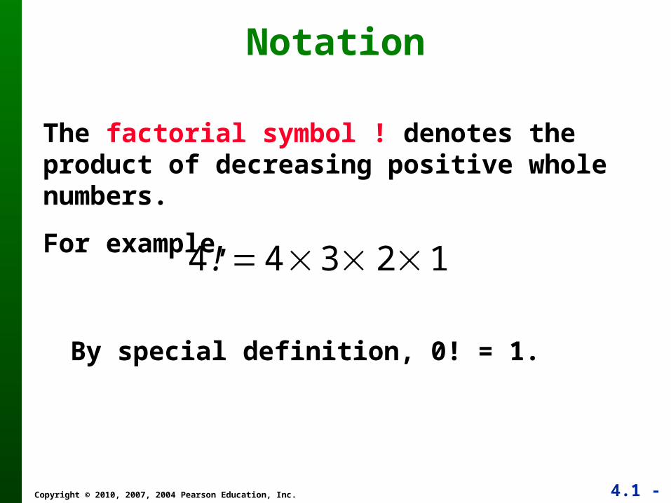
The factorial symbol ! denotes the product of decreasing positive whole numbers.

For example,

By special definition, 0! = 1.

4 != 4× 3× 2× 1


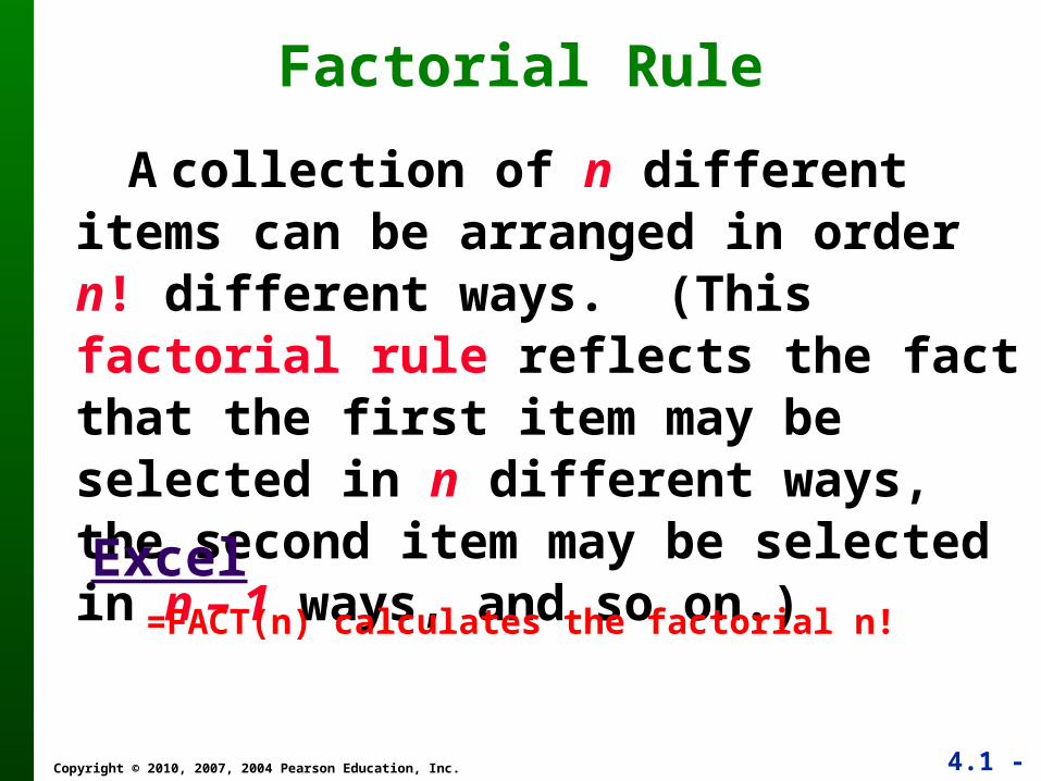
A collection of n different items can be arranged in order n! different ways. (This factorial rule reflects the fact that the first item may be selected in n different ways, the second item may be selected in n – 1 ways, and so on.)

Factorial Rule

=FACT(n) calculates the factorial n!

Excel


When different orderings of the same items are to be counted separately, we have a permutation problem, but when different orderings are not to be counted separately, we have a combination problem.

Permutations versus Combinations


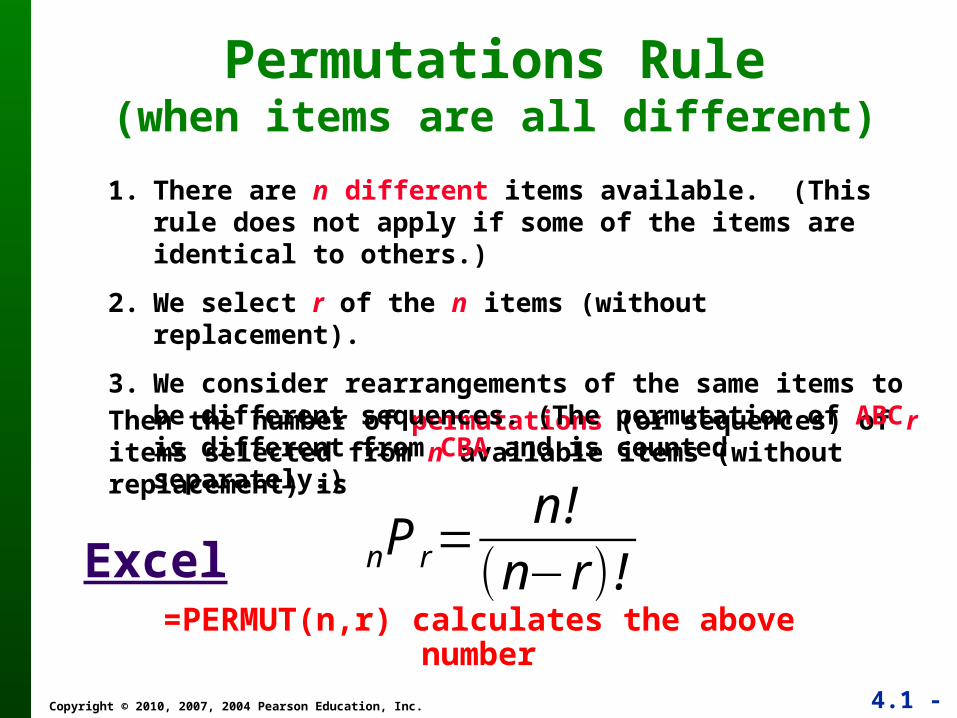
Permutations Rule(when items are all different)

Then the number of permutations (or sequences) of r items selected from n available items (without replacement) is

1. There are n different items available. (This rule does not apply if some of the items are identical to others.)

2. We select r of the n items (without replacement).

3. We consider rearrangements of the same items to be different sequences. (The permutation of ABC is different from CBA and is counted separately.)

=PERMUT(n,r) calculates the above number

Excel P rn =n !

(n−r)!


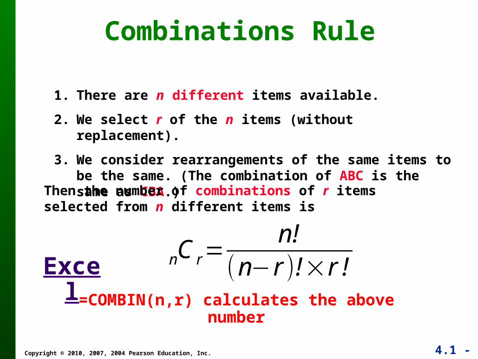
Combinations Rule

1. There are n different items available.

2. We select r of the n items (without replacement).

3. We consider rearrangements of the same items to be the same. (The combination of ABC is the same as CBA.)

Then the number of combinations of r items selected from n different items is

Excel=COMBIN(n,r) calculates the above number

C rn =n!

(n−r )!×r !

Documents

4.1 - 1 Copyright © 2010, 2007, 2004 Pearson Education, Inc. Section 4-2 Basic Concepts of Probability