4 · Web viewthe number of regimes between normals and supers, 4. the boundaries of the regimes between normals and supers, 5. the adjustment of regime boundaries to provide "zero"

4.5 Definition of Emission Regime Boundaries

In the old CALIMFAC model there was only one set of regime boundaries (Table 4-25) which did not change by model year groupings. In EMFAC2000, Sierra staff was asked to analyze the entire data set to determine if it was appropriate to continue with one set of regime boundary definitions or have them change by model year groupings.

Table 4-25 Regime boundary Definitions used in the CALIMFAC Model

Regime HC CO NOxNormal < 1x < 1x < 1xModerate >1-< 2x >1-< 2x >1-< 2xHigh >2-< 5x >2-< 6x >2-< 3xVery High >5-< 9x >6-< 10x >3-< 4xSuper >9x >10x >4x

In addition, Sierra staff was also charged with the task of determining if the super emission regime should be further sub-divided into super and super-super emission regimes. Following is the regime boundary analysis.

4.5.1 Regime Boundaries

This section discusses the steps used to determine the final regime boundaries for EMFAC2000. This is the first step in the development of a regime-based emission model. The following data sets were used in this analysis:

The old master data used for CALIMFAC, The new ARB surveillance data set, and Data from the I&M recapture fleet obtained in 1991 (2S91V1 and 2S91V2).

The regime boundaries apply to both the non-I&M and the with I&M fleet. Thus, it is appropriate to use the new ARB surveillance data set, which has vehicles, which have been through one or more I&M cycles. The I&M recapture data set was used at the suggestion of ARB staff as an additional data set that would be representative of fleet data in the determination of regime boundaries. In order to obtain large sample sizes for this analysis the regime boundaries were not determined for individual technology groups. Instead the analyses were done for three model-year groups: pre-1975, 1975 to 1979, and 1980 and later. These model year groups are surrogates for three broad classes of emission control technology: non-catalyst (pre-1975), oxidation catalyst (1975-1979), and three-way catalyst (1980-and-later). The regime boundaries are determined on the basis of emission ratios. These are the ratio of the measured emissions to the corresponding emission standard for the vehicle. This allows the consideration of vehicles with different emission standards in a given model year group.

Vehicles were grouped into regimes ranging from normal vehicles (the lowest emission group) to super emitters (the highest emission group). Specific steps required determining each of the following:

1. the upper boundary for normal vehicles,2. the lower boundary for super emitters,3. the number of regimes between normals and supers,4. the boundaries of the regimes between normals and supers,5. the adjustment of regime boundaries to provide "zero" slopes of

regression lines within each region (except normals), and

The descriptions provided below detail the specific data sets and methods used in each step.

4.5.1.2 Determination of the Upper Limit for the Normal Regime

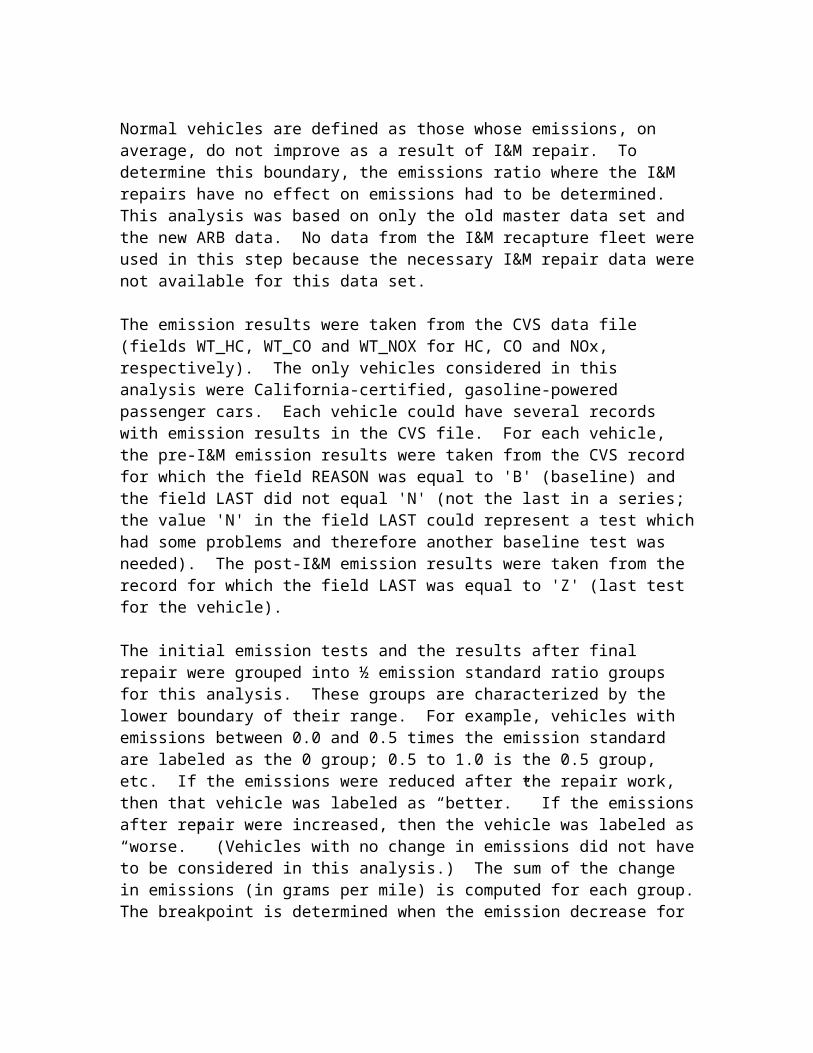
Normal vehicles are defined as those whose emissions, on average, do not improve as a result of I&M repair. To determine this boundary, the emissions ratio where the I&M repairs have no effect on emissions had to be determined. This analysis was based on only the old master data set and the new ARB data. No data from the I&M recapture fleet were used in this step because the necessary I&M repair data were not available for this data set.

The emission results were taken from the CVS data file (fields WT_HC, WT_CO and WT_NOX for HC, CO and NOx, respectively). The only vehicles considered in this analysis were California-certified, gasoline-powered passenger cars. Each vehicle could have several records with emission results in the CVS file. For each vehicle, the pre-I&M emission results were taken from the CVS record for which the field REASON was equal to 'B' (baseline) and the field LAST did not equal 'N' (not the last in a series; the value 'N' in the field LAST could represent a test which had some problems and therefore another baseline test was needed). The post-I&M emission results were taken from the record for which the field LAST was equal to 'Z' (last test for the vehicle).

The initial emission tests and the results after final repair were grouped into ½ emission standard ratio groups for this analysis. These groups are characterized by the lower boundary of their range. For example, vehicles with emissions between 0.0 and 0.5 times the emission standard are labeled as the 0 group; 0.5 to 1.0 is the 0.5 group, etc. If the emissions were reduced after the repair work, then that vehicle was labeled as “better.” If the emissions after repair were increased, then the vehicle was labeled as “worse.” (Vehicles with no change in emissions did not have to be considered in this analysis.) The sum of the change in emissions (in grams per mile) is computed for each group. The breakpoint is determined when the emission decrease for the better group is greater than the emission increase for the worse group.

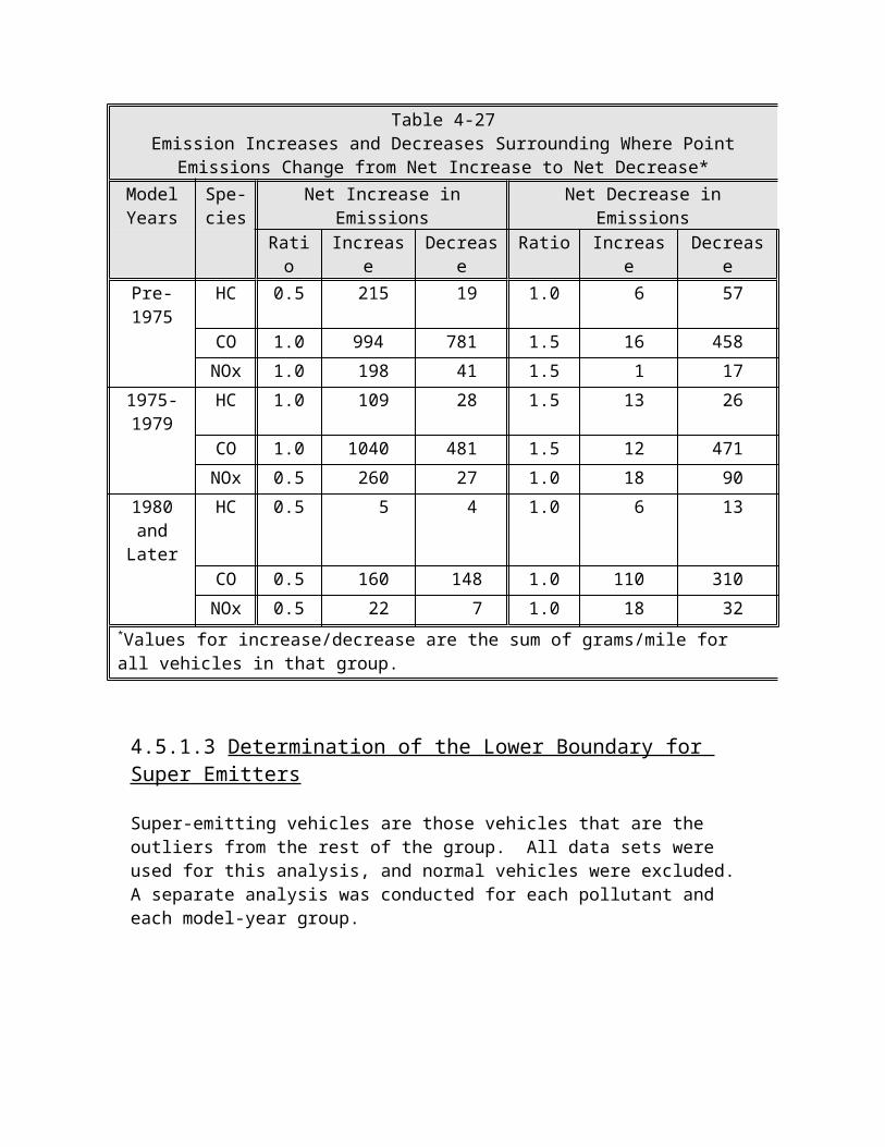
The results of this analysis are shown in Tables 4-26 and 4-27. Table 4-26 shows the breakpoints at which the emissions improved by the I&M repairs. Table 4-27 shows the results for emission increases and decreases for this group and the lower group where emission increases were greater than decreases. These breakpoints were usually near an emission ratio of 1.0 where the measured emissions equal the FTP standard. This range is intuitively reasonable in that the vehicles were designed to operate below the emission standard limit. In addition, the analysis for CALIMFAC also selected an emission ratio of 1.0 for the upper limit of normals.

There is no consistent pattern suggesting a change in the choice for the limit on normals. Accordingly, the boundary ratio for normal vehicles was retained at an emission ratio of 1.0 for all pollutants and all model years.

Table 4-26Normal Regime Breakpoints

Model Years HC CO NOx

Pre-1975 1.0 1.5 1.5

1975-1979 1.5 1.5 1.0

1980 and Later 1.0 1.0 1.0

Table 4-27Emission Increases and Decreases Surrounding Where Point Emissions Change from Net

Increase to Net Decrease*Model Years

Spe-cies

Net Increase in Emissions Net Decrease in Emissions

Ratio Increase Decrease Ratio Increase Decrease

Pre-1975 HC 0.5 215 19 1.0 6 57

CO 1.0 994 781 1.5 16 458

NOx 1.0 198 41 1.5 1 17

1975-1979

HC 1.0 109 28 1.5 13 26

CO 1.0 1040 481 1.5 12 471

NOx 0.5 260 27 1.0 18 90

1980 and Later

HC 0.5 5 4 1.0 6 13

CO 0.5 160 148 1.0 110 310

NOx 0.5 22 7 1.0 18 32*Values for increase/decrease are the sum of grams/mile for all vehicles in that group.

4.5.1.3 Determination of the Lower Boundary for Super Emitters

Super-emitting vehicles are those vehicles that are the outliers from the rest of the group. All data sets were used for this analysis, and normal vehicles were excluded. A separate analysis was conducted for each pollutant and each model-year group.

The procedure for identifying the outliers was adapted from a suggested procedure in the SAS manual.1 The initial step uses the SAS procedure FASTCLUS to create ten clusters for each pollutant/model-year group. This is done by setting the maximum clusters to ten and zero iterations (MAXC=10 and MAXITER=0).

The high-frequency clusters (i.e., those with the highest number of vehicles) that are found in the FASTCLUS procedure are less likely to contain the outlying data points. A cut point for "high-frequency" clusters is determined by examining the distribution of the number of vehicles in each cluster shown in the FASTCLUS output. This cutpoint typically includes 60-80% of the vehicles. The means from this group of high-frequency clusters are used as input to the next clustering step.

The next step also uses the FASTCLUS procedure. The same set of vehicle emission data is input, as well as the means of the high frequency clusters determined from the initial step. In this step, the number of clusters is set to two and the maximum cluster radius (the STRICT parameter) is specified. The specification of two clusters and the input of the high-frequency cluster means causes FASTCLUS to select the minimum and maximum values of the initial high-frequency cluster means as the seeds for the two clusters. The value specified for the STRICT parameter is determined from an examination of the output from the initial step. This output includes a plot of the distances between the clusters and cluster radii. The "typical" size of a cluster in this plot is used to establish the value used for the STRICT parameter.

The two clusters that are formed about the selected cluster seeds within the cluster radius set by the strict parameter contain the majority of the vehicles. The outlying vehicle with the lowest emissions ratio is taken as the boundary value for super-emitters. * A bar graph of the emissions grouped around multiples of the FTP standard is used to visually check the relation of the super emitters to the rest of the emissions distribution.

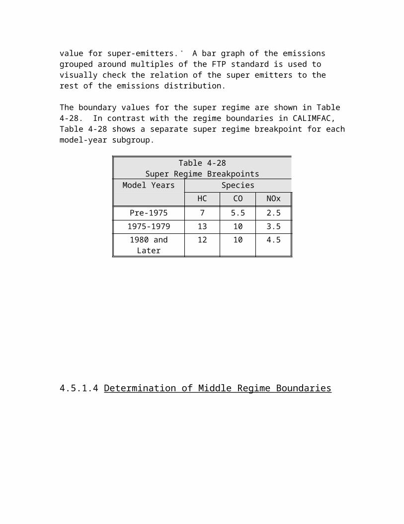
The boundary values for the super regime are shown in Table 4-28. In contrast with the regime boundaries in CALIMFAC, Table 4-28 shows a separate super regime breakpoint for each model-year subgroup.

Table 4-28Super Regime Breakpoints

1SAS/STAT User's Guide, Vol. 1, Version 6, Fourth Edition, page 842. Example 2: Outliers.

Model Years Species

HC CO NOx

Pre-1975 7 5.5 2.5

1975-1979 13 10 3.5

1980 and Later 12 10 4.5

4.5.1.4 Determination of Middle Regime Boundaries

This step used all the available data sets to determine the number and boundaries of the middle regimes. The data were divided into the same technology subgroups by pollutant and model year. The number of intermediate regimes was determined by using the SAS procedure CLUSTER. The procedure for identifying the number of clusters was adapted from a procedure in the SAS manual.2 The only non-default input parameter is the specification of Ward's method (METHOD=WARD). *

The output of this procedure includes the cubic clustering criterion (CCC), and the pseudo F and pseudo t2 statistics for the number of potential clusters. Starting from one potential cluster and then analyzing larger number of clusters, the first relatively higher value (peak) of the CCC or pseudo F statistic determines the number of clusters. For the pseudo t2 value, the first low value (valley) provides the likely number of clusters. If all three statistics give the same value for the number of potential clusters, then it is easy to determine the number of clusters. With the data used in this project, rarely do the three statistics yield the same value.3

There are no satisfactory methods for determining the number of population clusters for any type of cluster analysis. ... The number-of-clusters problem is, if anything, more difficult than the number-of-factors problem. Table 4-29 lists the values interpreted from these three clustering statistics. Typically, the range of possible clusters is between 2 and

2SAS/STAT User's Guide, Vol. 1, Version 6, Fourth Edition, page 588. Example 3: Cluster Analysis of Fisher Iris Data.

3

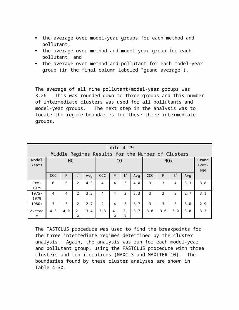
5. Because none of the three methods is any more significant than the others, the average of the three methods is chosen for a particular model year and pollutant. Table 4-29 shows these average values as well as the following averages:

the average over model-year groups for each method and pollutant, the average over method and model-year group for each pollutant, and the average over method and pollutant for each model-year group (in the final column

labeled "grand average").

The average of all nine pollutant/model-year groups was 3.26. This was rounded down to three groups and this number of intermediate clusters was used for all pollutants and model-year groups. The next step in the analysis was to locate the regime boundaries for these three intermediate groups.

Table 4-29Middle Regimes Results for the Number of Clusters

ModelYears

HC CO NOx GrandAverage

CCC F t2 Avg CCC F t2 Avg CCC F t2 Avg

Pre-1975 6 5 2 4.3 4 4 3 4.0 3 3 4 3.3 3.8

1975-1979

4 4 2 3.3 4 4 2 3.3 3 3 2 2.7 3.1

1980+ 3 3 2 2.7 2 4 3 3.7 3 3 3 3.0 2.9

Average 4.3 4.0 2.0 3.4 3.3 4.0 2.7 3.7 3.0 3.0 3.0 3.0 3.3

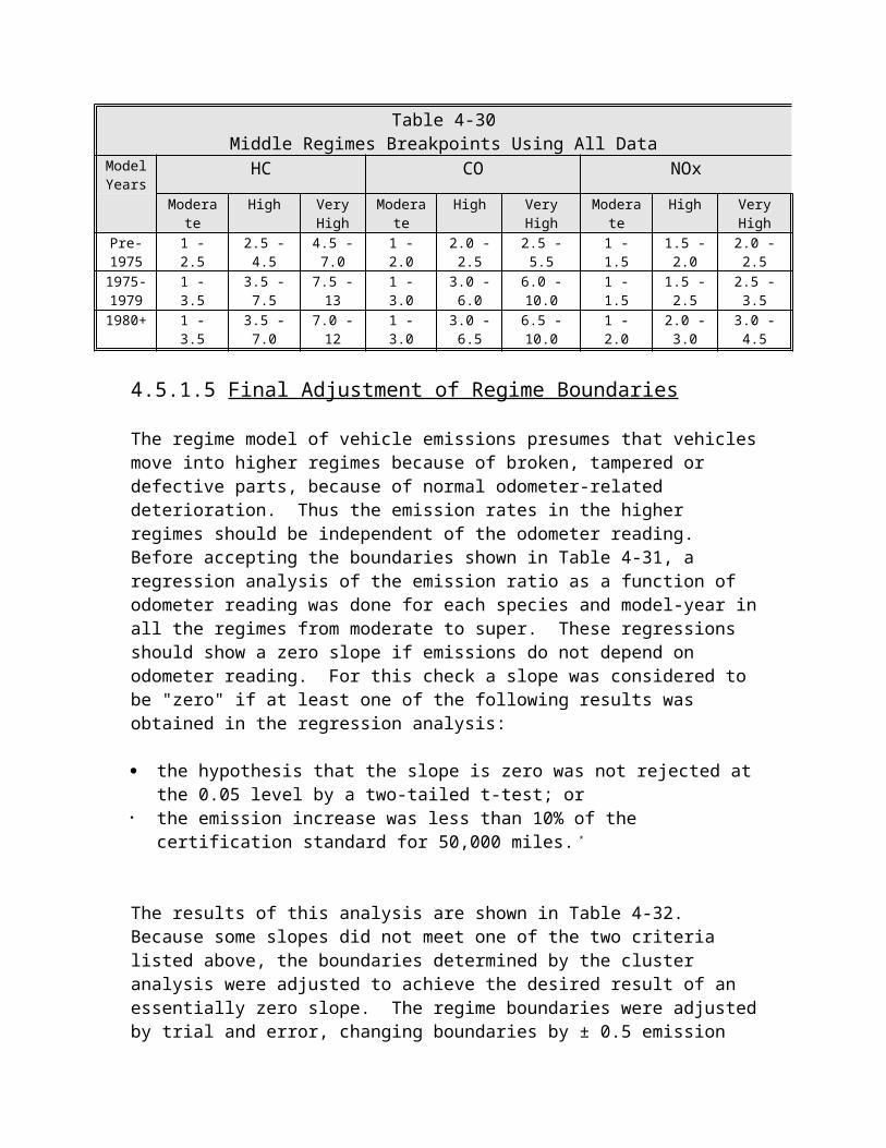
The FASTCLUS procedure was used to find the breakpoints for the three intermediate regimes determined by the cluster analysis. Again, the analysis was run for each model-year and pollutant group, using the FASTCLUS procedure with three clusters and ten iterations (MAXC=3 and MAXITER=10). The boundaries found by these cluster analyses are shown in Table 4-30.

Table 4-30Middle Regimes Breakpoints Using All Data

Model Years

HC CO NOx

Moderate High Very High

Moderate High Very High Moderate High Very High

Pre-1975

1 - 2.5 2.5 - 4.5 4.5 - 7.0 1 - 2.0 2.0 - 2.5 2.5 - 5.5 1 - 1.5 1.5 - 2.0 2.0 - 2.5

1975-1979

1 - 3.5 3.5 - 7.5 7.5 - 13 1 - 3.0 3.0 - 6.0 6.0 - 10.0 1 - 1.5 1.5 - 2.5 2.5 - 3.5

1980+ 1 - 3.5 3.5 - 7.0 7.0 - 12 1 - 3.0 3.0 - 6.5 6.5 - 10.0 1 - 2.0 2.0 - 3.0 3.0 - 4.5

4.5.1.5 Final Adjustment of Regime Boundaries

The regime model of vehicle emissions presumes that vehicles move into higher regimes because of broken, tampered or defective parts, because of normal odometer-related deterioration. Thus the emission rates in the higher regimes should be independent of the odometer reading. Before accepting the boundaries shown in Table 4-31, a regression analysis of the emission ratio as a function of odometer reading was done for each species and model-year in all the regimes from moderate to super. These regressions should show a zero slope if emissions do not depend on odometer reading. For this check a slope was considered to be "zero" if at least one of the following results was obtained in the regression analysis:

the hypothesis that the slope is zero was not rejected at the 0.05 level by a two-tailed t-test; or

the emission increase was less than 10% of the certification standard for 50,000 miles. *

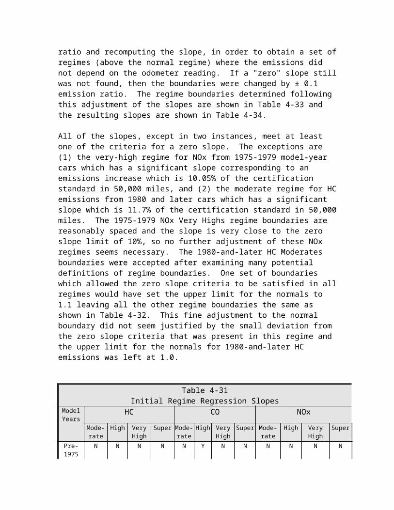
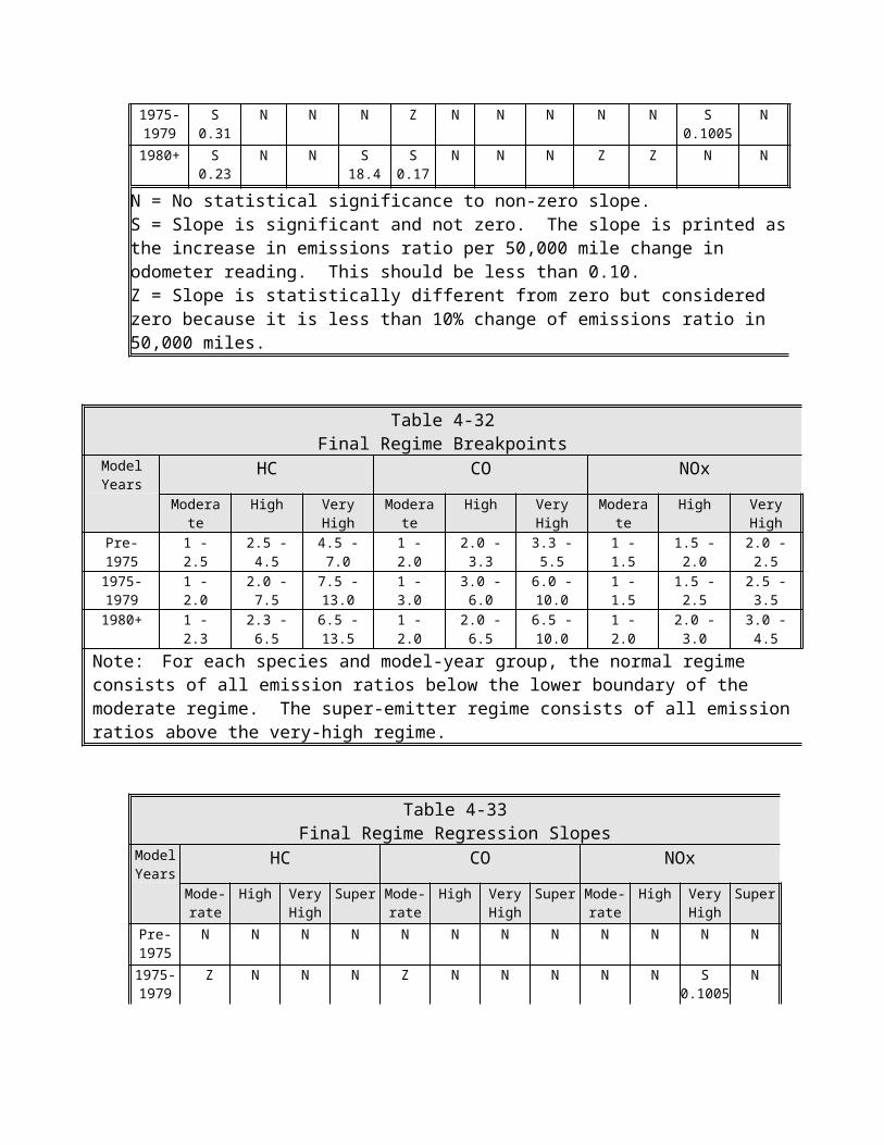
The results of this analysis are shown in Table 4-32. Because some slopes did not meet one of the two criteria listed above, the boundaries determined by the cluster analysis were adjusted to achieve the desired result of an essentially zero slope. The regime boundaries were adjusted by trial and error, changing boundaries by ± 0.5 emission ratio and recomputing the slope, in order to obtain a set of regimes (above the normal regime) where the emissions did not depend on the odometer reading. If a "zero" slope still was not found, then the boundaries were changed by ± 0.1 emission ratio. The regime boundaries determined following this adjustment of the slopes are shown in Table 4-33 and the resulting slopes are shown in Table 4-34.

All of the slopes, except in two instances, meet at least one of the criteria for a zero slope. The exceptions are (1) the very-high regime for NOx from 1975-1979 model-year cars which has a significant slope corresponding to an emissions increase which is 10.05% of the certification standard in 50,000 miles, and (2) the moderate regime for HC emissions from 1980 and later cars which has a significant slope which is 11.7% of the certification standard in 50,000 miles. The 1975-1979 NOx Very Highs regime boundaries are reasonably spaced and the slope is very close to the zero slope limit of 10%, so no further adjustment of these NOx regimes seems necessary. The 1980-and-later HC Moderates boundaries were accepted after examining many potential definitions of regime boundaries. One set of boundaries which allowed the zero slope criteria to be satisfied in all regimes would have set the upper limit for the normals to 1.1 leaving all the other regime boundaries the same as shown in Table 4-32. This fine adjustment to the normal boundary did not seem justified by the small deviation from the zero slope criteria that was present in this regime and the upper limit for the normals for 1980-and-later HC emissions was left at 1.0.

Table 4-31Initial Regime Regression Slopes

Model Years

HC CO NOx

Mode-rate

High Very High

Super Mode-rate

High Very High

Super Moderate High Very High Super

Pre- 1975 N N N N N Y N N N N N N

1975-1979

S 0.31 N N N Z N N N N N S 0.1005 N

1980+ S 0.23 N N S 18.4 S 0.17 N N N Z Z N N

N = No statistical significance to non-zero slope.S = Slope is significant and not zero. The slope is printed as the increase in emissions ratio per 50,000 mile change in odometer reading. This should be less than 0.10.Z = Slope is statistically different from zero but considered zero because it is less than 10% change of emissions ratio in 50,000 miles.

Table 4-32Final Regime Breakpoints

Model Years

HC CO NOx




Pre-1975 1 - 2.5 2.5 - 4.5 4.5 - 7.0 1 - 2.0 2.0 - 3.3 3.3 - 5.5 1 - 1.5 1.5 - 2.0 2.0 - 2.5

1975-1979

1 - 2.0 2.0 - 7.5 7.5 - 13.0 1 - 3.0 3.0 - 6.0 6.0 - 10.0 1 - 1.5 1.5 - 2.5 2.5 - 3.5

1980+ 1 - 2.3 2.3 - 6.5 6.5 - 13.5 1 - 2.0 2.0 - 6.5 6.5 - 10.0 1 - 2.0 2.0 - 3.0 3.0 - 4.5

Note: For each species and model-year group, the normal regime consists of all emission ratios below the lower boundary of the moderate regime. The super-emitter regime consists of all emission ratios above the very-high regime.

Table 4-33Final Regime Regression Slopes

Model Years

HC CO NOx

Mode-rate

High Very High

Super Mode-rate

High Very High

Super Mode-rate

High Very High

Super

Pre- 1975

N N N N N N N N N N N N

1975-1979

Z N N N Z N N N N N S 0.1005

N

1980+ S .117 N N N Z N N N Z Z N N

N = No statistical significance to non-zero slope.S = Slope is significant and not zero. The slope is printed as the increase in emissions ratio per 50,000-mile change in odometer reading.Z = Slope is statistically different from zero but considered zero because it is less than 10% change of emissions ratio in 50,000 miles.

4.5.2 Regime Growth Rates

This section outlines the approach taken in the development of regime growth functions. The EMFAC2000 model is based on the distribution of vehicles among the various emission regimes. This distribution is determined in two steps. First, the change in regime populations as vehicles age, without an inspection/maintenance (I&M) program, is modeled. This aging process results in a shift of vehicles from the normal regime into regimes with higher emissions. The growth in the population of the higher-emitting regimes is described by the regime growth functions discussed in this section.

There are two potential measures of vehicle “age”: the odometer reading, and the estimated time the vehicle has been in customer service as determined from the difference between the test date and model year. Both of these variables play a role in the regime growth. To the extent that some deterioration of emission control systems is due to weathering effects, the regime growth would be best characterized by vehicle age. To the extent that deterioration is due to vehicle use, the regime growth would be best characterized by the odometer reading. EMFAC2000 uses a fixed distribution of vehicle age to odometer reading so only one of these variables can be used in determining the population of the various regimes. The average relation between vehicle age and odometer reading shows that the average vehicle is driven fewer miles per year as it ages. Consequently, a nonlinear relation between either of these variables and regime population sizes would represent the combined effects of both.

A major issue in the development of regime growth functions is the data requirement for different regime populations as a function of vehicle age or odometer reading. The data analysis problems can be illustrated by considering a hypothetical technology group with 500 vehicles. This would appear to present enough data points, but these 500 vehicles are distributed into each of the five emission regimes. Although this provides an average of 100 vehicles in each regime, there is usually a high concentration of vehicles in the normal and moderate regimes and a much smaller number in the very high and super regimes. The average of 100 vehicles per regime for the hypothetical technology group must next be subdivided into odometer (or age) groups. Typically intervals of 10,000 miles or one year are used to group the variables. This typically provides 20 mileage bins

or 10 year bins with an average of five or ten vehicles per bin. These final five or ten vehicles are then used to compute the individual regime population data points used in the regression equations.

4.5.2 Analysis

The regime growth functions represent the movement of vehicles among emission regimes in the absence of an I&M program. Consequently, the derivation of these functions uses only data for vehicles that have not been through an I&M program. The data used in this analysis are the same data used for the regime growth functions in CALIMFAC, augmented by some EPA data for 49-state vehicles. None of the recent ARB surveillance data, which were for vehicles that had been through I&M, were used.

In CALIMFAC, linear regression equations between mileage and regime population sizes were used for the regime growth functions. As an initial step in developing regime growth functions for EMFAC2000, the regime populations for the technology groups with the largest number of vehicles (old technology groups four, six, eight, nine, and eleven) were plotted on a series of charts for visual detection of any apparent relations with mileage and age. The regime populations were determined using 10,000-mile bins, 25,000-mile bins, and one-year bins. A separate chart was prepared for each regime and each pollutant. Each chart contained 15 graphs showing all three methods for binning the data for each of the five technology groups selected. Although there was significant scatter in these charts, a general nonlinear trend was evident in both the mileage- and age-based plots. Accordingly, nonlinear functions were used for regime growth functions of all technology groups, and some preliminary efforts were made to examine different nonlinear regime growth functions.

The regime growth functions were determined based on the vehicle odometer reading. (Since vehicle emission factor models use a fixed relationship between vehicle age and odometer, either parameter can be used in a nonlinear relation.) For a given pollutant and technology group, the following procedure was followed in obtaining population data for the regime growth functions.

1. The data were grouped into 10,000-mile "bins": (0-10,000), (10,001-20,000) etc. The mileage for each bin was represented by its midpoint odometer value. The total number of vehicles in each bin was determined. This number was used to weight the data in the following step.

2. For each bin, the number of vehicles in each regime (normal, moderate, high, very high, and super) was determined. This number was then divided by the total number in that bin to get the fraction of vehicles in each regime in the bin.

3. Regression analysis was applied to data on the population fraction of each regime as a function of odometer reading at the midpoint of the population bin. (For convenience, the reading was divided by 10,000 miles.)

A simplified example of this procedure is provided below to clarify the individual steps in computing the population distributions and regression weights. For purposes of this

example, 25,000 mile bins are used in place of 10,000 mile bins and an upper limit of 100,000 miles is used. The normal upper limit was the maximum odometer reading observed in the sample.

Table 4-34 contains the hypothetical distribution, for a particular pollutant and technology group, of the number of vehicles over regime and odometer range. These data are used to compute the population distributions as a function of the midpoint of the odometer range as shown in Table 4-35. The data in this table were used in the regression analysis for regime growth functions.

Table 4-34Hypothetical Distribution of Vehicles by Regime and

Odometer Range

Odometer Range (miles)

Regime0-

25,00025,001-50,000

50,001-75,000

75,001-100,000

Normal 24 98 11 1

Moderate 2 7 13 4

High 0 2 11 5

Very high 0 0 4 2

Super 0 1 6 4

Total 26 108 45 16

The regime growth function used a weighted analysis where the weight for each mileage bin (i.e., the last row in Table 4-34) was taken as the total number of vehicles in the mileage bin. This step of the procedure was independent of the regression approach used; it simply provided the basic data for those regressions.

Table 4-35Hypothetical Regime Populations Distributions as a

Function of Mileage

Regime

Bin Midpoint Mileage (miles/10,000)

1.25 3.75 6.25 8.75

Normal 92.3% 90.7% 24.4% 6.3%Moderate 7.7% 6.5% 28.9% 25.0%High 0.0% 1.9% 24.4% 31.3%

Very high 0.0% 0.0% 8.9% 12.5%Super 0.0% 0.9% 13.3% 25.0%

Two basic approaches were used to model nonlinear regime growth functions: the first examined the use of functions that could not be transformed into a linear function, and the second was based on linear regression. For the first approach, the SAS procedure, NLIN, was used to determine the regression coefficients A, B, C, and D in the following relation between regime-i population, pi, and the odometer reading, (odo).

Pi = A + B*(odo) + C*e D(odo) [4-4]

The regression equations produced by this approach did not provide statistically significant values for C or D. In general, the values for C were small and/or the values for D were large negative numbers. The resulting equations amounted to little more than a linear equation with a slight correction at lower mileage. This approach was not used for the final regime growth functions.

A second set of preliminary studies used the stepwise regression procedure of the SAS procedure REG. In order to allow for different possible regression lines, including a linear relation (i.e., one with constant slope) and nonlinear curves with either increasing slope or decreasing slope, the following regression equation was used:

Pi = A + B*(odo) + C* (odo)2 + D*(odo)1/2 [4-5]

Initially two sets of regressions were performed. One set used bins with a constant mileage interval. A second set of regressions used variable width bins with the same number of vehicles in each bin. * For this process, an ideal bin population of fifty vehicles was selected. However, if necessary due to data limitations, regressions were carried out with as few as four bins containing at least twenty vehicles per bin. As noted above, weighted regressions were used for the constant width bins to account for the different number of vehicles in each bin. Such weighting was not required for the variable width bins. A comparison of these two approaches showed no difference in the results and the constant width bin regressions were used in the final analysis.

One additional regression procedure was evaluated to overcome a major problem with the development: the lack of data at high mileage. This is illustrated in Figure 4-1 which shows the distribution of vehicle odometer readings in the total data set used for determining regime growth functions. Although there were variations from this overall distribution in each technology group, the general pattern of this figure--a sharp drop in available data with increasing mileage--was observed in all technology groups.

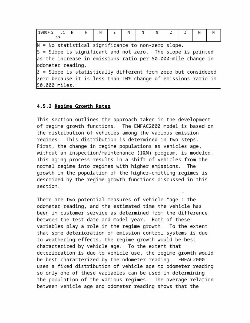
Figure 4-1 Odometer Distribution in Regime Growth Function Data

The attempted improvement in regressions at high mileage used the following approach. Appropriate aggregations ("super-groups") of technology groups, with similar characteristics, were formed, and regressions were developed for these super groups. These regressions were then used to obtain the high mileage regime populations for each technology group within the super-group. In this approach, the usual regime growth function for the technology group, pi,G(odo) was used for odometer readings below 100,000 miles. Above 100,000 miles, the regime growth was found from the regression for the super-group using the following equation:

Pi,G (odo) = Pi,G (100,000 mi) + Pi,G (odo) – Pi,SG(100,000 mi) [4-6]

where pi,SG is the regime growth function for the super-group. This approach did not provide any apparent improvement over the regressions using all the data and was not pursued further.

Regressions were carried out for all regimes. In the CALIMFAC model, the population of the normal regime is not found from regression equations; instead, it is determined by subtracting the populations of all other regimes from 100%. With the use of nonlinear regression functions, the regression curve for normals was typically proportional to the square root of the odometer reading. This gave a steep initial drop, with a declining slope. The population of normals persisted longer than was the case when it was computed as the difference between 100% and the populations of all other regimes. A rough check on the persistence of normals was done by examining the combined data for all technology groups with odometer readings above 140,000 miles. The regime populations for the 24 vehicles in this highest mileage range are shown in Table 4-36.

0.00%

2.00%

4.00%

6.00%

8.00%

10.00%

12.00%

14.00%

16.00%

0-10k 10-20k

20-30K

30-40k

40-50k

50-60k

60-70k

70-80k

80-90k

90-100k

100-110k

110-120k

120-130k

130-140k

140-150k

over150k

Mileage Range

Perc

ent i

n M

ileag

e Ra

nge

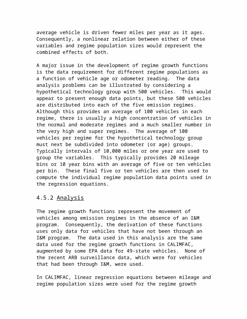
Table 4-36Regime Populations at High Mileage for Combined Data Set

Species

Percent of Vehicles in the Following Regimes

Normal Moderate High Very High Super

HC 8.3 54.2 20.8 4.2 12.5CO 16.7 45.8 16.7 8.3 12.5

NOx 29.2 50.0 12.5 8.3 0.0

The persistence of a significant population of normals, even in the highest mileage bin, is best accounted for by always using the regression equation for normals and then adjusting the population of all regimes so that they total 100%. This change was made in EMFAC2000 so that the overall approach for computing the regime populations was done in the following steps.

1. Regression equations were used to compute the raw regime populations for all five regimes.

2. Any negative regime fraction was set to zero. Any regime fraction greater than one was set to one.

3. The regime fractions determined in step 2 were summed. This sum was then divided into each regime fraction from step 2 to obtain a final set of regime fractions, which summed to one.

A similar approach was used to determine the regression equations for the raw regime population data.

4.5.2.1 Final Regime Growth Functions

The final regime growth functions were determined using the SAS regression procedure, REG, using the "adjusted R-squared" method. This method computes regression results for all possible combinations of variables. For the regression equation considered here [A + B(odo) + C(odo)2 + D(odo)1/2 ], seven different regression equations are possible. These are listed below with the abbreviations for each regression and a list of the terms set to zero.

Linear term only (Linear: C = D = 0)Quadratic term only (Quadratic: B = D = 0)Square-root term only (SQRT: B = C = 0)Linear and quadratic terms (L/Q: D = 0)Linear and square-root terms (L/SQRT: C = 0)Quadratic and square-root terms (Q/SQRT: B = 0)All terms

Prior to a selection of the final regression equation plots were made which overlaid all the regression equations and the data used as the basis of those equations. The population data points used to form the regressions generally show a large scatter, especially at high mileage where there were very few vehicles. In the high-mileage region, there might be only one vehicle in a particular 10,000-mile bin. The population of whatever regime in which this vehicle happened to lie was 100%; the population of all other regimes was zero. This variation did not have a significant effect on the regressions because the weight assigned to these points (i.e., the ratio of vehicles in this mileage bin compared to the total number of vehicles) was small.

Comparison of various regression equations showed a region between approximately 20,000 and 120,000 miles where the populations predicted by different regression results were very close. In this region, the variation in the predictions was less than the scatter in the data points. The regression, which resulted from using all variables typically, has both a minimum and a maximum did not seem to represent real vehicle behavior. In addition, this curve often extends well above 100% and well below zero. Similar eccentric behavior was noted for regression results with two variables.

The adjusted R2 was used as a measure to compare various regression fits because this variable is a measure of the explanatory power of the model adjusted for the number of parameters in the regression equation. * In most cases the regression results with more than one variable had a somewhat higher value for R2 than the one-variable equations, but they had a lower value for R2

adj. In general, the equations, which had the highest value of the adjusted R2, appeared to have the most plausible physical behavior. Consequently the initial choice of a regression equation (from the seven possible alternatives) was the one with the highest value of the adjusted R2.

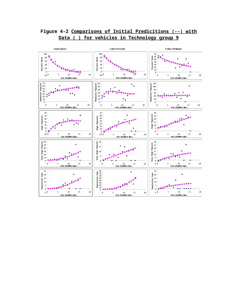
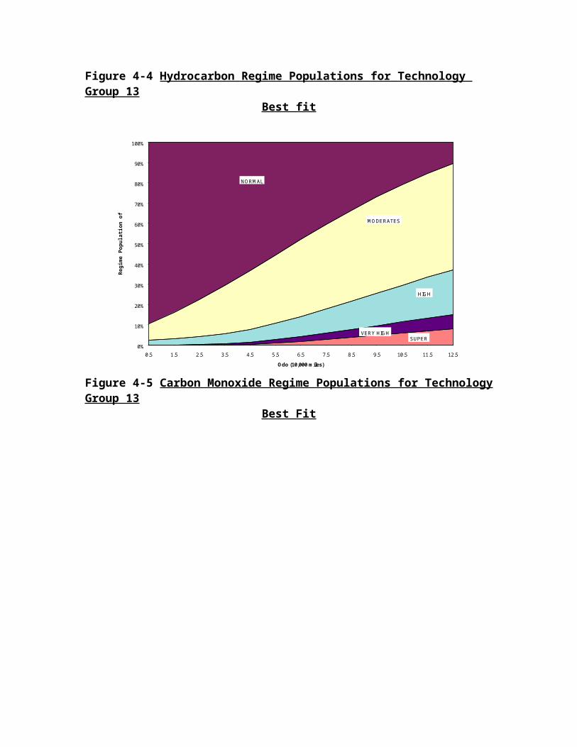
The initial choice of a regression equation for each regime produced the “best” equation for that regime. Once an initial set of regression equations was selected for each regime the full EMFAC2000 calculation procedure was applied to the regression results. (Initial regression values less than zero were set to zero; values greater than one were set to one; the resulting regime fractions were renormalized so that the sum of all regime populations was one.) The resulting regime populations were then compared to the actual data on regime populations. For example, Figure 4-2 shows the results of the initial selection of regime growth functions for technology group nine. In this case the agreement between the population data and the regime growth functions (as used in EMFAC2000) was considered adequate and no modifications were made. Another example is shown in Figure 4-3: the initial regime growth functions for technology group thirteen. Some slight changes were made in the selection of regime growth functions shown in this figure. These substitutions are shown in Table 4-37. The regime growth functions for each pollutant are shown in Figures 4-4 to 4-6.

Table 4-37Adjustments Made in Regime Growth Functions for Technology Group Thirteen

Pollutant Regime Initial Equation Final Equation

Type Adjusted R2 Type Adjusted R2

HC Moderate Linear/Sqrt 0.73 Linear 0.59

HC High Sqrt 0.49 Quadratic 0.38

CO Moderate Sqrt 0.48 Linear 0.45

NOx Normal Quadratic 0.43 Linear 0.36

The procedure illustrated here for technology groups eight and thirteen was repeated for all other technology groups. In some cases where the number of vehicles in a particular technology group/regime combination was small aggregation of technology groups were used to derive the regime growth functions. For example, the regime growth functions for the very high and super regimes in technology groups one, two and three (non-catalyst vehicles) were obtained by aggregating the data for all three technology groups.

Figure 4-2 Comparisons of Initial Predicitions (--) with Data ( ) for vehicles in Technology group 9

Hydrocarbons Carbon Monoxide Oxides of Nitrogen

-20

0

20

40

60

80

100

0 5 10 15 20

Odo (10,000 miles)

Perc

ent N

orm

al

010203040506070

0 5 10 15 20Odo (10,000 miles)

Mod

erat

e Po

pula

tion

-10

0

10

20

30

40

50

60

0 5 10 15 20odo (10,000 miles)

High

Pop

ulat

ion

0

10

20

30

40

50

60

0 5 10 15 20Odo (10,000 miles)

Very

Hig

h Po

pula

tion

-5

0

5

10

15

20

25

0 5 10 15 20

Odo (10,000 miles)

Popu

latio

n Su

pers

-20

0

20

40

60

80

100

0 5 10 15 20

Odo (10,000 miles)

Perc

ent N

orm

al0

10

20

30

40

50

60

0 5 10 15 20Odo (10,000 miles)

Mod

erat

e Po

pula

tion

-100

10203040506070

0 5 10 15 20odo (10,000 miles)

High

Pop

ulat

ion

0

5

10

15

20

0 5 10 15 20Odo (10,000 miles)

Very

Hig

h Po

pula

tion

01020304050607080

0 5 10 15 20Odo (10,000 miles)

Popu

latio

n Su

pers

010203040506070

0 5 10 15 20Odo (10,000 miles)

Perc

ent N

orm

al

0

20

40

60

80

100

120

0 5 10 15 20Odo (10,000 miles)

Mod

erat

e Po

pula

tion

0

5

10

15

20

25

30

0 5 10 15 20odo (10,000 miles)

High

Pop

ulat

ion

-5

0

5

10

15

20

25

30

0 5 10 15 20Odo (10,000 miles)

Very

Hig

h Po

pula

tion

-5

0

5

10

15

20

25

0 5 10 15 20

Odo (10,000 miles)

Popu

latio

n Su

pers

Figure 4-3 Comparisons of Initial Predictions (--) with Data ( ) for vehicles in Technology group 13

Hydrocarbons Carbon Monoxide Oxides of Nitrogen

-20

0

20

40

60

80

100

120

0 5 10 15 20Odo (10,000 miles)

Perc

ent N

orm

al

-40-20

020406080

100120

0 5 10 15 20

Odo (10,000 miles)

Mod

erat

e Po

pula

tion

0

10

20

30

40

50

0 5 10 15 20odo (10,000 miles)

High

Pop

ulat

ion

02468

10121416

0 5 10 15 20Odo (10,000 miles)

Very

Hig

h Po

pula

tion

-10

0

10

20

30

40

50

60

0 5 10 15 20Odo (10,000 miles)

Popu

latio

n Su

pers

-20

0

20

40

60

80

100

120

0 5 10 15 20Odo (10,000 miles)

Perc

ent N

orm

al

0

20

40

60

80

100

120

0 5 10 15 20Odo (10,000 miles)

Mod

erat

e Po

pula

tion

-10

0

10

20

30

40

50

60

0 5 10 15 20odo (10,000 miles)

High

Pop

ulat

ion

0

2

4

6

8

10

12

0 5 10 15 20Odo (10,000 miles)

Very

Hig

h Po

pula

tion

-5

0

5

10

15

20

0 5 10 15 20

Odo (10,000 miles)

Popu

latio

n Su

pers

0

20

40

60

80

100

120

0 5 10 15 20Odo (10,000 miles)

Perc

ent N

orm

al

0

20

40

60

80

100

120

0 5 10 15 20Odo (10,000 miles)

Mod

erat

e Po

pula

tion

0

2

4

6

8

10

12

0 5 10 15 20odo (10,000 miles)

High

Pop

ulat

ion

-1

0

1

2

3

4

5

6

0 5 10 15 20Odo (10,000 miles)

Very

Hig

h Po

pula

tion

-1

0

1

2

3

4

5

0 5 10 15 20

Odo (10,000 miles)

Popu

latio

n Su

pers

Figure 4-4 Hydrocarbon Regime Populations for Technology Group 13 Best fit

Figure 4-5 Carbon Monoxide Regime Populations for Technology Group 13Best Fit

0%

10%

20%

30%

40%

50%

60%

70%

80%

90%

100%

0.5 1.5 2.5 3.5 4.5 5.5 6.5 7.5 8.5 9.5 10.5 11.5 12.5

Odo (10,000 miles)

Reg

ime

Popu

latio

n of

HC

NORMAL

MODERATES

HIGH

VERY HIGHSUPER

0%

10%

20%

30%

40%

50%

60%

70%

80%

90%

100%

0.5 1.5 2.5 3.5 4.5 5.5 6.5 7.5 8.5 9.5 10.5 11.5 12.5

Odo (10,000 miles)

Reg

ime

Popu

latio

n of

CO

NORMAL

MODERATE

HIGH

VERY HIGH

SUPER

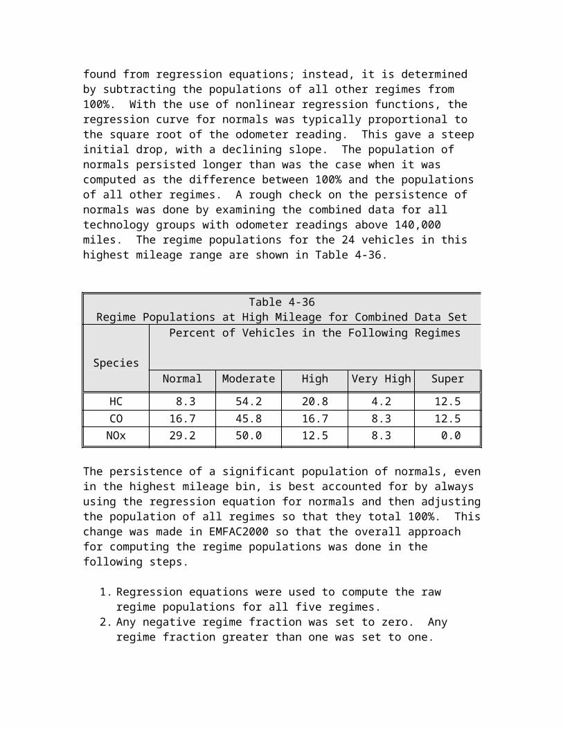
Figure 4-6 Oxides of Nitrogen Regime Populations for Technology group 13Best Fit

0%

10%

20%

30%

40%

50%

60%

70%

80%

90%

100%

0.5 1.5 2.5 3.5 4.5 5.5 6.5 7.5 8.5 9.5 10.5 11.5 12.5

Odo (10,000 miles)

Reg

ime

Popu

latio

n of

NO

x

NORMAL

MODERATE

HIGHVERY HIGH

SUPER

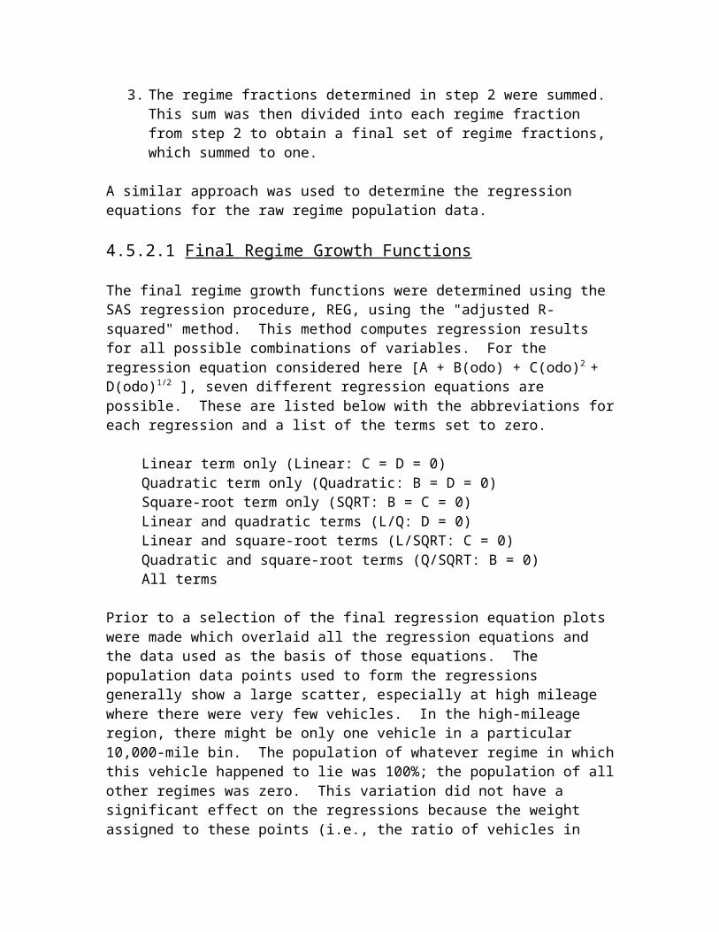
Table 4-38Coefficients in Regime Growth Functions

Regime Population = A + B(odo) + C(odo)2 + D(odo)1/2

Population in percent; odo is odometer reading divided by 10,000Technology

GroupSpecies Regime Constant

Term, ALinear

Term, BQuadraticTerm, C

Square RootTerm, D

1 HC Super 0.428 0 0.01767 0Very High

-3.389 0 0 2.4998

High 0 0 0 0.3052Moderate 43.647 1.9853 0 0Normal 52.174 -3.1158 0 0

CO Super 0 0 0 0.402Very High

-3.868 0 0 3.138

High 7.927 0 0 0.159Moderate 33.227 0 0 0.891Normal 61.436 0 0 -3.977

NOx Super 0 0 0 0.6758Very High

-3.8676 0 0 3.1384

High 0 0 0 1.0158Moderate 32.474 0 0 -1.266Normal 60.907 0 0 1.307


-3.389 0 0 2.4998

High 0 0 0 0.3052Moderate 17.451 0 0 8.424Normal 64.159 -1.3339 0 0


-3.868 0 0 3.138

High 0 1.058 0 0Moderate 27.983 0 0.02441 0Normal 48.913 0 0 3.776


0.707 0 0 3.722

High 4.603 0 0 2.236Moderate 33.022 0 0 -3.725Normal 44.045 0.999 0 0

3 HC Super 0.428 0 0.01767 0Very -3.389 0 0 2.4998

HighHigh 2.714 7.5129 0 0Moderate 54.365 0 0 -11.368Normal 50.068 -4.8012 0 0


-3.868 0 0 3.1381

High 9.967 0 0 0Moderate 32.902 0 0 2.231Normal 77.119 0 0 -14.626


-3.8676 0 0 3.1384

High 7.102 0 0 4.8558Moderate 36.525 -1.6606 0 0Normal 57.83 0 0 -3.138

4 HC Super -0.696 0 0 0.782Very High

-0.241 0.3179 0 0

High -3.648 6.061 -0.10103 0Moderate 2.534 0 0 10.124Normal 116.492 0 0 -30.979

CO Super -0.058 0 0 1.3703Very High

0.412 1.3588 0 0

High 2.615 1.3583 0 0Moderate -5.035 0 0 17.3458Normal 110.81 0 0 -29.2072

NOx Super 0.061 0 0 0.2342Very High

0 0 0 2.6151


5 HC Super -0.939 1.264 0 0Very High

-1.391 1.392 0 0

High -11.254 -2.41 0 34.947Moderate 40.265 0 0 -8.405Normal 144.998 34.7909 -0.85724 -127.941


-1.745 0 0 7.334

High -15.135 0 0 18.849

Moderate 41.129 0 0 -4.1292Normal 96.069 4.9052 0 -45.6392

NOx Super -1.997 0.7657 0 0Very High

0 0 0 2.4872

High 4.9742 0 0 8.3095Moderate 14.2364 2.9509 0 0Normal 82.7382 0 0 -18.8475

6 HC Super -0.896 1.142 0 0Very High

-1.286 1.255 0 0

High -11.562 -1.884 0 31.237Moderate 36.608 0 0 -5.121Normal 78.357 0 0 -27.825


-2.175 0 0 6.822

High -0.363 4.7024 0 0Moderate 33.511 0 0 -2.3115Normal 100.37 4.1974 0 -42.001


0 0 0 2.4872

High 3.418 0 0 8.177Moderate 15.653 2.3847 0 0Normal 82.969 0 0 -17.1854


-0.412 0.549 0.0625 0

High -10.857 0 0 17.465Moderate 26.937 -6.425 0 23.79Normal 70.119 0 0 -22.716

CO Super 0.199 0 0.02732 0Very High

0.06 0 0.12311 0

High 0.196 1.726 0 0Moderate 0.691 0 0 12.545Normal 94.651 -8.855 0.23218 0


1.785 0 0 1.371

High 6.649 1.8667 0 0Moderate 26.834 -3.0758 0.32051 0Normal 75.761 0 0 -9.467


1.926 0 0.10092 0

High 3.64 4.7051 0 0Moderate 24.647 0 0 5.2535Normal 85.97 0 0 -28.8098

CO Super -4.77 2.0799 0 0Very High

-3.19 0 0 3.4864

High -1.115 4.1257 0 0Moderate 0.306 0 0 14.9346Normal 85.273 -8.1636 0 0

NOx Super -2.8554 0 0 2.6358Very High

-4.1839 0 0 4.0035


9 HC Super -0.137 0 0.06136 0Very High

0.608 0 0.11437 0

High -15.862 0 -0.10084 18.1976Moderate 20.46 0 0 8.5061Normal 122.339 5.2094 0 -53.4096

CO Super 0.77 -0.7768 0.24325 0Very High

0.084 0.8392 0 0

High -14.89 0 0 14.97Moderate -17.798 -14.3809 0.24848 52.322Normal 110.159 0 0 -31.1218


-4.278 0 0 4.0389



-0.776 0.5236 0 0

High -1.864 2.0374 0 0Moderate -11.979 0 0 14.45Normal 128.071 0 0 -27.7418

CO Super -1.213 0 0 2.798Very -3.123 1.1648 0 0

HighHigh -17.225 0 0 13.074Moderate 16.151 0 0 7.952Normal 143.146 7.039 0 -60.409


-0.13 0.2783 0 0

High 0.539 0 0.06592 0Moderate 13.45 0 0.15456 0Normal 84.897 0 -0.24025 0


0 0 0 2.1878

High -3.339 2.8571 0 0Moderate 5.927 0 0 14.209Normal 107.45 0 0 -29.3827


-1.879 0.4656 0 0

High 4.041 0 0.20882 0Moderate 6.753 2.4039 0 0Normal 115.792 0 0 -25.034

NOx Super 0 0 0 0Very High

-2.491 0 0 2.6

High -9.744 0 0 10.5918Moderate 9.604 0 0 16.3178Normal 102.631 0 0 -29.5096


0 0 0 2.3655

High -4.204 2.8345 0 0Moderate 13.76 3.9987 0 0Normal 118.253 0 0 -33.685


-2.372 0.5564 0 0



-1.982 0 0 2.815

High -5.572 0 0 9.837

Moderate 7.117 0 0 16.704Normal 100.436 0 0 -29.356


0.03 0 0.0574 0

High 2.91 0 0.1574 0Moderate 7.251 4.3863 0 0Normal 153.377 4.3249 0 -52.8213


0.371 0 0.02884 0



0 0 0 0

High 1.525 0 0.03028 0Moderate 5.802 0 0.24022 0Normal 98.817 -2.871 0 0


-0.778 0.5213 0 0



-8.387 0 0 5.142

High -17.18 0 0 13.015Moderate 15.349 0 0 8.303Normal 111.433 0 0 -29.243


-0.403 0.3686 0 0



0.0255 0 0.05553 0

High 3.011 0 0.15284 0Moderate 7.736 4.46 0 0Normal 134.047 0 0 -34.3017


0.3553 0 0.0279 0



-0.59 0.2649 0 0



2.252 0 0.02768 0



-5.75 0 0 3.9185

High 0.186 4.5518 0 0Moderate -0.25 0 0 13.134Normal 87.02 -8.0337 0 0

NOx Super -0.174 0 0.02143 0Very High

-1.611 0 0 1.5451


4.5.2.2 Additional Changes to the Regime Growth Rates

During beta testing of EMFAC2000, the fleet average FTP based emission rates were compared to data collected during BAR’s random roadside tests. These comparisons revealed that the HC and CO rates calculated by EMFAC2000, for 1985 and newer model years were higher than those observed in the random roadside sample. Conversely, the NOx rates were lower than those observed in the random roadside sample for the same years.

Sierra staff was asked to review the basic emission rates, and determine the probable cause of these emission differences. Sierra staff noted that in the development of the regime growth rates, EPA data were classified into the regimes using Federal certification standards instead of the California certification standards. This resulted in potential high emitters being classified as normal emitters. The regime growth rates for technology groups 9, 10, 12 and 13 were revised. Table 4-39 shows the revised regime growth rates.

Table 4-39 Revised Regime Growth Rates

Tech. Group

Species Regime Intercept A

Linear B

Quadratic C

Square Root D

9 HC Normal 101.002 0 0 -30.8359Moderate 16.875 7.6004 -0.4684 0High -8.279 0 0 12.8909Very High 0.608 0 0.11437 0Super -0.137 0 0.06136 0

CO Normal 76.125 -5.3415 0 0Moderate 20.266 0 0 4.7454High -10.996 0 0 11.8972Very High 0.463 0 0.06282 0Super 0.069 0 0.09332 0

NOx Normal 74.753 0 0 -16.6521Moderate 42.283 0 -0.03903 0High 1.953 1.5443 0 0Very High -4.468 0 0 4.7021Super -1.703 1.2579 0 0

10 HC Normal 103.857 -6.2008 0 0Moderate -17.243 0 0 15.5692High -2.575 1.9662 0 0Very High 0.126 0 0.04756 0Super -1.963 0 0 1.8398

CO Normal 125.757 0 0 -21.1541Moderate -11.308 0 0 10.1092High -1.877 1.2748 0 0Very High -2.399 0 0 1.8767Super -3.711 0 0 3.1843

NOx Normal 88.123 -4.7844 0 0Moderate 0.69 0 0 13.3924High 2.212 0 0.02082 0Very High -0.91 0 0.09309 0Super 0.152 0 0.03301 0

12 HC Normal 105.898 0 0 -29.2096Moderate 5.74 0 0 14.9709High -11.858 0 0 10.942Very High 4.966 0 0 0.1715Super -0.628 0 0.06733 0

CO Normal 111.264 0 0 -22.6882Moderate 3.026 0 0 9.6354High -9.46 0 0 7.0193Very High -0.787 0 0.04424 0Super -1.63 0 0 4.1078

NOx Normal 100.568 0 0 -26.8723Moderate 13.275 0 0 13.2327High -9.447 0 0 9.8849Very High -0.637 0.8346 0 0Super 0 0 0 0

13 HC Normal 109.046 -6.5884 0 0Moderate -25.539 0 0 20.124High -2.737 1.4625 0 0Very High -0.283 0 0.04918 0Super -0.372 0.1617 0 0

CO Normal 105.743 -3.5649 0 0Moderate 1.425 0 0.17265 0High -0.925 0.6891 0 0Very High -0.72 0.4792 -0.03283 0Super -1.278 0.5484 0 0

NOx Normal 95.246 -4.6266 0 0Moderate 9.326 2.8196 0 0High -0.216 0 0.07875 0Very High -0.498 0.3305 0 0Super -0.651 0 0.04112 0

Documents

4 · Web viewthe number of regimes between normals and supers, 4. the boundaries of the regimes between normals and supers, 5. the adjustment of regime boundaries to provide "zero"