Embed Size (px)
Citation preview

'4' THE SYNTHESIS.: OF
REDUNDANTMULTIPLE - LINE
>" NETWORKS
~ First Annual Report
* ~Contract Nonr 3842(00)
May 1, 1963
Prepared by
P.A. JensenW.C. MannM. R. Cosgrove
IAI
I7WESTINGHOUSE ELECTRIC CORPORATION J
ELECTRONICS DIVISIONADVANCED DEVELOPMENT ENGINEERING
P.O. Box 1897 Baltimore 3, Maryland

First Annual Report
Contract Nonr 3842(00)
For the Period March 1, 1962 to May 1, 1963
THE SYNTHESIS OF REDUNDANT
MULTIPLE-LINE NETWORKS
A
May 1, 1963
Prepared for
Office of Naval Research
byWestinghouse Electric Corporation
Electronics Division
P.O. Box 1897
Baltimore 3, Maryland
Prepared by: Approved by:
P.A. Jensen . , Director
W.C. Mann
M. R. Cosgrove
TPE 4482

ABSTRACT
This report describes a synthesis technique for redundant multiple-line networks which
determLies the optimum placement of restorers for minimum cost. The cost expression is
a function of system reliability, cost of implementation, weight, power, and speed. The re-
dundant networks are required to have the same order of redundancy throughout, but other-
wise the form of the network is restricted very little by the synthesis procedure. The
procedure is developed in sufficient detail for application to sample networks and for imple-
mentation on a computer.
A prime requisite to the synthesis procedure is a means for predicting the reliability
of multiple-line redundant networks. A new technique for performing this operation is pre-
sented in this report. It is applicable to multiple line networks of almost any configuration.
JI __ __ _ __ _ __I__ __l
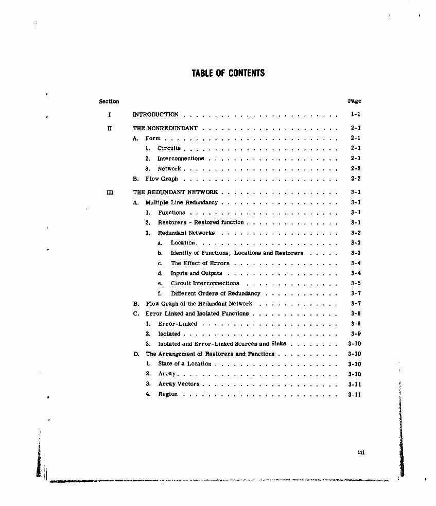
TABLE OF CONTENTS
Section Page
I INTRODUCTION. .. ......... ........... .... 1-1
II THE NONREDUNDANT .. .... ........... ....... 2-1
A. Form .. ... .......... ............ ... 2-1
1. Circuits .. .. .......... .......... ... 2-1
2. Interconnections .. .... ........... ...... 2-1
3. Network .. .. ......... ........... ... 2-2
B. Flow Graph. .. .......... ........... ... 2-2
III THE REDUNDANT NETWORK .. .. ........... ...... 3-1
A. Multiple Line Redundancy .. .. ........... ...... 3-1
1. Functions. .. ........ ........... .... 3-1
2. Restorers - Restored function .. .. .......... ... 3-1
3. Redundant Networks. ... ........... ...... 3-2
a. Location .. .. ....... ........... ... 3-3
b. Identity of Functions, Locations and Restorers. .. .... 3-3
c. The Effect of Errors .. .... ............. 3-4
d. Inpu,'ts and Outputs. .. .......... ....... 3-4
e. Circuit Interconnections .. ......... ...... 3-5
f. Different Orders of Redundancy .. ..... ....... 3-7
B. Flow Graph of the Redundant Network .. ....... ...... 3-7
C. Error Linked and Isolated Functions. .. ....... ...... 3-8
1. Error-Linked .. ..... ........... ...... 3-8
2. Isolated. .. ..... ........... ......... 3-9
3. Isolated and Error-Linked Sources and Sinks. .. ........ 3-10
D. The Arrangement of Restorers and Functions. .. ......... 3-10
1. State of a Location. .. ....... ............ 3-10
2. Array. .. ... ........... ........... 3-10
3. Array Vectors. .. ...... .......... .....- 11
4. Region. .. ......... ........... .... 3-11

TABLE OF CONTENTS (Continued)
Section Page
IV THE SYNTHESIS OF REDUNDANT NETWORKS ... ............ ... 4-1
A. General .......... ............................ .. 4-1
B. Optimization Criterion ....... ..................... .. 4-2
C. The Isolating Array Synthesis Procedure ...... ............. 4-3
1. A General Description of the Procedure ............... ... 4-4
2. The Effect of a Restorer ...... .................. .. 4-5
a. Reliability ......... ....................... 4-6
b. Functional Cost ....... .................... .4-10
c. Determination of the Optimum State of the Location . . .. 4-11
d. Isolating Arrays and Isolated Regions .............. .. 4-12
3. The Approximation in the Procedure ..... ............. 4-13
a. The Quantity Minimized ...... ................ .. 4-13
b. Calculation of the Region Cost .... .............. .4-15
c. The Effect of the Approximation on the Optimum ........ 4-16 i
4. The Detailed Procedure ....... ................... 4-17
D. Some Emample Results of the Procedure .... ............. .4-26
V CONCLUSIONS AND RESULTS ....... ................... ... 5-1
LIST OF APPENDICES
APPENDIX A. DETERMINATION OF THE RELIABILITY OF MULTIPLE LINENETWORKS
APPENDIX B. GENERATING THE ISOLATING ARRAYS
APPENDIX C. GENERATING THE ISOLATED REGIONS FROM THEISOLATING ARRAYS
iv

LIST OF ILLUSTRATIONS
Figure Title Page
2-1 An Example of a Nonredundant Network ....... ............... 2-1
2-2 Flow Graph Representation of the Nonredundant Network of
Figure 2-1 ......... ........................... .... 2-2
3-1 The Transformation from a Nonredundant circuit to a Redundant
Function ............. ........................... 3-1
3-2 Restorer of a Multiple-Line Network .... ............... .... 3-2
3-3 Order 3-Multiple-Line Redundant Network ... ............. .... 3-3
3-4 Erroneously Interconnected Functions .... ............... .... 3-5
3-5 Function with Direct Feedback from Output to Input .. ......... ... 3-6
3-6 Function with Direct Feedback with a Restorer on its Output ..... ... 3-6
3-7 Flow Graph Representing a Redundant Network ..... ........... 3-7
3-8 A Network in which Functions 3 and 4 are Isolated ............. ... 3-9
3-9 A Network is which Functions 1 and 2 are Isolated from Functions
3, 4, 5and.6 ........ .......................... .... 3-94-1 The Effect of a Restorer in a Shift Register ...... ............. 4-6
4-2 The Networkthat must be Considered when Determining the Effect
of a Restorer in Location 5 ....... ................... ... 4-10
4-3 Network Containing Two Indivisible Isolated Regions ........... ... 4-15
4-4 Example Network for the Detailed Procedure ...... ............ 4-17
4-5 Example Network with the Functions Identified ... ........... ... 4-17
4-6 The Isolated Region of the Isolating Array of the First Function
( ?, 1, x, 0, 1, x) ....... ....................... .... 4-19
4-7 The Isolated Region of Figure 4-6 with Location 1 taking on its two
Possible States ........... ......................... 4-19
4-8 Optimum Design of the Network ...... .................. ... 4-25
v/vi

I. INTRODUCTION
Every electronic component is subject to failure. Modern technology has reduced the
rate of this failure to extremely low levels. As modern warfare and data processing require
machines which perform more and more sophisticated tasks, industry responds with extremely
complex equipment requiring prodigious numbers of parts. Since a nonredundant machine
requires the correct functioning of all its components, the individual small probabilities of
failure accumulate to yield a very significant probability of failure for the eouipment, causing
an average time between failures of only a matter of hours. For the repairable machine, this
means down time while repair is effected. For the nonrepairable machine, such as might be
found in an unmanned orbital satellite or a ballistic missile guidance system, it means failure
of a mission.
Often the down time associated with repair or the failure of a mission cannot be allowed
or, at least, is extremely expensive. To overcome failure of modern electronic equipment, the
use of redundancy has been proposed. In general, the term redundancy refers to extra equip-
ment incorporated into the system which is above and beyond the minimum required to imple-
ment the task. This additional equipment is merged into the system such that failures are
masked or overcome and the system operation is maintained even though a number of circuit
failures have occurred.
This study has dealt with multiple-line redundancy which is described in detail in Sec-
tion III of this report. Westinghouse has studied several schemes for incorporating circuit
redundancy into digital machines, and this has been found to be the most effective.
Multiple-line redundancy operates, in parallel, a number of replicas of each circuit in
the nonredundant network. The number of replicas of a circuit is its order of redundancy.
Groups of circuits called restorers, whose sole purpose is the correction of errors which
arise due to circuit failures, are placed at various points in the network. The redundancy
of circuits plus the restorers provide a network with an ability to withstand a number of cir-
cuit failures without impairment of its operation.
Past studies by Westinghouse. and a number of other investigations, have shown that
multiple-line redundancy is indeed a valid approach to increasing the reliability of electronic
equipment. This study is devoted to establishing procedures with which the designer can
determine the best way to incorporate redundancy. It seeks to answer the question, "Given
the nonredundant network, the reliability and cost of all its parts and the reliability and cost
of restorers, what is the optimum way to assign redundancy to the circuits and what is the
optimum way to place restorers in the network?" This is the problem of synthesis.
1-1

The first step toward a procedure to perform synthesis is the proposal of factors which
are to be considered in determining whether one network design is better than another. This
study has combined the factors of cost of the circuits in the network, reliability, weight,
power, and speed into a ringle criterion for optimization which is called the True Cost. The
network which has the minimum True Cost is the optimum network.
The most obvious approach to finding the optimum network design is to try all the alter-
natives, measuring their True Costs, and picking out the most inexpensive design. Unfortu-
nately, the number of alternatives one has to consider increases so rapidly with the size of
the network that this exhaustive search approach is eminently impracticable for all but the
smallest networks. What is desired from this study is a synthesis procedure which is deter-
ministic, in that it gives the network that minimizes the True Cost, and which can be per-
formed in a reasonable amount of time with the aid of a computer.
This report introduces a procedure called the "Isolating Array Synthesis Procedure"
which uses a characteristic of multiple-line networks to considerably reduce the number of
calculations from the amount required for exhaustive search. At this point in the study, the
same number of replicas must be provided for all circuits. The procedure is deterministic,
but there are approximations inherent in its operation, and the result may not be the design
which minimizes the True Cost. The approximations are small, however, and for most prob-
lems, the True Cost of the result of the Procedure will be very little greater than the minimum
True Cost. The approximations are justified by the considerable savings in effort that are
available through the use of the procedure. The result of this study is a significant contribu-
tion and is the first means proposed for finding the optimum arrangement of restorers short
of an exhaustive search.
A prime requisite to any synthesis procedure is a technique for analyzing the reliabi-
lity of multiple-line networks. Unfortunately, the analysis techniques developed in the past
required the networks to have a regularity uncommon to real networks; hence, they could not
be used for the synthesis procedure. This study develops a reliability analysis procedure
which is applicable, with few restrictions, to any multiple-line network. This procedure, pre-
sented in Appendix A, is a useful contribution to the study of redundant networks.
1-2

II. THE NONREDUNDANT NETWORK
A. FORM
The techniques developed in this report are applicable to general networks with as few
restrictions as possible on the type of circuits that make up the network or the pattern of
interconnections between the circuits. To illustrate the tyre of network under study, a non-
redundant sample is shown in figure 2-1.
Figure 2-1. An Example of a Nonredundant Network
1. Circuits
The numbered squares in figure 2-1 are digital circuits. They operate on binary
information at their inputs to produce binary information at their outputs. Although the com-
plexity of the circuits is not strictly limited in the procedures, the most exact representation
of the network results if the circuits are as simple as possible, performing basic logical opera-
tions such as AND, OR, NOR, NOT or the sequential functions of flip flops or other memory
devices. Circuits may have any number of inputs but only one output. An output may be split
to provide network outputs or inputs to as many other circuits as required by the network.
It is not necessary that the circuits be alike.
2. Interconnections
There are no restrictions on the interconnection of circuits in the network. Any
circuit output may be a network output and/or provide inputs to any circuit in the network.
In figure 2-1, the directed line segments show the Interconnections between circuits.
2-1

3. Network
For the nonredundant case the network is made up of circuits. The assumption ismade that each circuit must perform correctly for the network to operate. Since each circuit
performs some logical function, the network may also be described by the functions performed
by its circuits. For the redundant examples to follow, this convenience will often be used since
a function will be performed by a number of identical circuits.
The network may have any number of inputs from the "outside world" or outputs to
the "outside world."
B. FLOW GRAPH
The network can be described by a flow graph such as that shown in figure 2-2. The
vertices represent the functions or circuits and are numbered for identification. The directed
line segments represent connections between the circuits. A line segment into a vertex is an
input to the circuit and a line segment out of a vertex is an output of the circuit. In this re-port the flow graphs specify the form of the nonredundant network and are used to introduce
some terms that are peculiar to this paper. Special flow graphs will be introduced later
which describe redundant networks.
Figure 2-2. Flow Graph Representation of the Nonredundant Network of Figure 2-1
The flow graph example of figure 2-2 represents the network of figure 2-1. With the
help of this figure, several terms are described which find considerable application later
in the report.
A source of a circuit y is a circuit x such that the inputs of y depend logically on the
circuit x. A source is identified on the flow graph if a path can be traced from x to y in theforward direction along the directed line segments. For instance, the sources of circuit 6are circuits 1, 2, 3 and 5. By following the directed line segments from the inputs of thenetwork to circuit 6 through all possible routes, the reader will find that each of these cir-cuits is encountered. The sources are further subdivided according to their distance from
the circuit (the number of line segments that are traversed when going from a source to the
2-2

circuit). A primary source is acircuit directlyproviding aninput to the circuit. For instance,
the primary sources of circuit 6 are circuits 2 and 5. Secondary sources are the circuits
that directly provide the inputs to the primary sources, hence two line segments are traversed
when going from a secondary source to the circuit. For circuit 6, the secondary sources are
circuits 1 and 3. In general, n line segments are traversed in going from an nth-order source
to the circuit.
A circuit may have more than one order of source. For instance, circuit 1 is a second-
ary, tertiary and higher order source of circuit 6. In going from 1 to 6, two, three or more
segments may be traversed; either from I to 2 and from 2 to 6; from 1 to 3, 3 to 2, and 2 to
6; or from I to 2, 2 to 3, 3 to 2, 2 to 6; etc. The networks considered here are finite, and
while the order of a particular source may go to infinity, a circuit can have only a finite num-
ber of sources. at most, all the circuits in the network.
The interconnection topology of the network is completely specifie i by the sources of
its circuits.
An opposite concept to the source is the sink of a circuit. A sink of a circuit x is a
circuit y whose output logically depends on x. If y is a sink of x, then x is a source of y. In
figure 2-2, the sinks of circuit 2 are circuits 3, 4, and 6. Once again, a sink has an order
which depends on the number of line segments one must traverse when going in the forward
direction from the circuit to its sink. A primary sink of a circuit is connected directly to
its output. A secondary sink is connected directly to the output of a primary sink. In general,
n line segments are traversed in going from a circuit to one of its nth order sinks.
2-3/4

Ill. THE REDUNDANT NETWORK
A. MULTIPLE-LINE REDUNDANCY
The type of redundancy which is the subject of this report is one studied extensively by
Westinghouse and found to be one of the most efficient types of circuit redundancy 1' 2. This
section describes multiple-line redundancy with definitions of some of the terms used exten-
sively in this report.
1. Functions
In general, multiple-line redundancy is applied by replacing the single circuit of
the nonredundant network by m identical circuits operating in parallel. The group of circuits
is now called a function. The symbol m refers to the order of redundancy of the function.
Figure 3-1 shows this transformation.
NONREDUNDANT 1 REDUNDANTCICI F UNCTION
Figure 3-1. The Transformation from a Nonredundant Circuit to a Redundant Function
The function has m output lines, but since they are all carrying nominally the same
signal, the function is said to have one output carried on m lines. In like manner the func-
tion will have I inputs, each input carried on m lines.
2. Restorers- Restored Function
The reliability improvement expected with the use of redundant circuits depends
on the ability of the network to experience circuit failures without degradation of the network
operation. The use of restorers within the network provides this characteristic. A restorer
3-1

is shown in figure 3-2*. When the functions at the restorer's input and output are the same
order of redundancy, it has m inputs and m outputs. The inputs are the outputs of one func-
tion, and the outputs provide the inputs to one or more functions.
m FUNCTIONS
RESTORING CIRCUIT
Figure 3-2. Restorer of a Multiple-Line Network
The restorer consists of m restoring circuits which are the circles in figure 3-2.
If a restoring circuit is operating correctly it has the ability to derive the correct output if
k of its m inputs are correct. Working restoring circuits filter out errors on their inputs.
Theonly reasons for an erroneous output line of a restorer are the failure of a restoring cir-
cuit or the incidence of m - k + 1 or more errors on the inputs to the restorer. In the event
of the latter condition, all the restorer outputs become erroneous since the restoring circuits
are identical.
A function which has a restorer on its output is called a restored function. Errors
on the output of a restored function can be corrected if at least k of the m output lines carry
the correct information.
3. Redundant Networks
The redundant network is made up of redundant functions and restorers. An ex-
ample of order three multiple-line redundancy is shown in figure 3-3. This is the redundant
* Restorers may operate on the output lines of a function, as described in this section, or onthe input lines to a function, as described in references 1, 2 and 3. Studies at Westinghouseand at Hycon Eastern Incorporated3 indicate the former arrangement is most effective.
3-2

version of figure 1-1 with restorers placed after functions 2 and 5. For these restoring cir-
cuits k equals 2 and m equals 3; they are majority elements.
Figure 3-3. Order 3-Multiple-Line Redundant Network
Some general characteristics can be mentioned with the help of this illustration.
a. Location
The division of the network into functions requires that the circuits making up
a function have outputs which are amenable to restoration. In other words a restorer may,
if desired, be placed on the output of any function in a redundant network. A location is de-
fined here as a place in the network where restoration may be accomplished. Every outputof a redundant function is a location, and there is no location that is not an output of a re-
dundant function.
b. Identity of Functions, Locations and Restorers
With s functions in the network, numbers from 1 to s identify the functions.
This has been done in figure 3-3 where functions are numbered 1-6.
Since a location is associated with only one function, the number of the loca-
tion is the same as its function. For instance, the location on the output of function 1 in
figure 3-3 is called location 1.
When a restorer is placed in location y it is identified by the number s +y.
Thus, in this example in which s = 6, restorer 8, in location 2, operates on the output lines
of function 2 and restorer 11 operates on the output lines of function 5.
i 3-3
A particular circuit in a redundant function is identified by its position. The
lower case subscripts on the numerals identifying each circuit is the position of that circuit.
The symbol Ia refers to a circuit in function 1 in position a. Output lines of functions or
restorers also have positions determined by the position of the circuit from which it emanates.
Positions have been assigned to each circuit in figure 3-3.
c. The Effect of Errors
Circuits or networks that are operating correctly or lines which carry correct
information are said to be successful. The opposite states, incorrect operation or informa-
tion, are called failed.
Two assumptions on the effects of circuit failures are made for this report.
First, when a circuit (in a function or a restorer) fails, its output is always in error. Second-
ly, when a circuit in a function has an input which is in the failed condition, the output of that
circuit is failed. For instance, if circuit 1a is failed, its own output and the outputs of the
circuits 2, 3 and 4 are in error.
Restoring circuits will determine the correct output if k of their m inputs are
correct. For instance, if one of the circuits in function 2 has erroneous outputs and if none
of the members of restorer 8 are failed, there are no errors on the outputs of this restorer.
This report assumes that restoring circuit reliability is independent of whether its inputs
include failures. If the restoring circuit has at least k correct inputs, the probability that
its output is co.'rect or failed depends only on the reliability of the restoring circuit.
d. Inputs and Outputs
The inputs to the network are assumed error free.
At the outputs of the network there must be some means to reduce to a single
line the information carried by the multiple lines of the redundant network. This report
assumes that such a means is available and that only k of the m output lines need be success-
ful for the output to be successful. All the network outputs must fulfill this criterion for the
network to be operating successfully. For the example of figure 3-3, if at least two of the
outputs of both functions 4 and 6 are correct, this network has not failed.
The reliability of the multiple-line network is the probability, at a given time,
that, at each network output, at least k lines are successful. The reliability of the network is
a function of the reliabilities of the circuits in the network. It is assumed that the reliability
of a circuit is the probability that its output Is successful given its inputs are successful.
The reliability of a particular circuit is independent of the success or failure of any other
circuits. Appendix A provides a procedure with which the reliability of multiple-line net-
works can be determined.
3-4

Since the network output functions are restored they are classed as restored
functions. They are restored only for the network outputs however, not for any feedback
between a network output and some other function in the network.
e. Circuit interconnections
This section describes the manner in which the circuits in functions or re-
storers are interconnected in multiple-line networks. The principles described here are
characteristic of multiple-line networks and are not restrictions on the synthesis procedure.
Functions are interconnected in the manner shown in figure 3-3. The output
lines of a function provide the inputs directly to the circuits in other functions, as the circuits
in function 1 provide the inputs directly to the circuits of functions 2 and 3. Care must be
taken so that failure of one circuit in any function does not cause failure of two circuits in
another function. If functions 1, 2, and 3 were connected in the manner shown in figure 3-4,
this condition would be violated and any circuit failure in function 1, would cause two output
lines of function 2 to be in error disabling the system.
Figure 3-4. Erroneously Interconnected Functions
For instance if 1 fails, the inputs to 2 and 3 are in error disabling theira a a
outputs. But 3a provides an input to 2c , hence it too is in error. With 2 and 2c in error,
all the output lines of restorer 8 are in error and the system is failed.
The possibili*y of such an interconnection error can be eliminated if only cir-
cuits in the same position are interconnected. This rule does not apply to connections be-
tween a restored function and its restorer.
The connection between function 2 and restorer 8, infigure 3-3, shows how
these interconnections are made in multiple-line systems. Every circuit output line in the
restored function goes to every restoring circuit in the restorer.
3-5
F:

In the absence of restorer 8 the circuits in function 2 would be interconnected
to the circuits in functions 3 and 6. But when restorer 8 is added its output feeds functions 3
and 6, and the output lines of function 2 go only to the restorer. In general, the rule may be
stated that whenever a restorer is placed on the output of a function y in any redundant sys-
tem, the restorer feeds all other functions formerly fed by function y and function y feeds
only the restorer.
There is one exception to this rule. That is when there is a direct feedback
from a function's output to one of its inputs with no other functions in the feedback path. Such
a situation is shown in figure 3-5.
Figure 3-5. Function with Direct Feedback from Output to Input
When a restorer is placed on the output of this function, the feedback paths
should not be disturbed, as in figure 3-6.
Figure 3-6. Function with Direct Feedback with a Restorer on its Output
The reason for this exception is illustrated by noting the effect when circuit
Ya fails. Such an occurrence causes the restorer to have an erroneous input line and -a it-
self to have an erroneous input because of the feedback. Placing the feedback line after the
restorer would correct the input to ya' but its output line is still in error, and there i no
improvement. Placing the feedback after the restorer only increases the chance that the
feedback input to Y will be in error because of a restoring circuit failure.
3-6

Placing a restorer on the output of another restorer gives no increase in reli-
ability. In general, restorers follow only functions.
f. Different Orders of Redundancy
The most general multiple-line model would allow each function in the network
to take on any order of redundancy. This flexibility has been compromised in this report to
simplify the synthesis problem. For the synthesis technique all the functions in a network
are required to have the same order of redundancy. The removal of this restriction will be
the subject of future studies.
For the analysis technique to be described in Appendix A, greater flexibility
has been allowed. These generalizations are described in that Appendix with rules for inter-
connecting different orders of redundancy.
B. FLOW GRAPH OF THE REDUNDANT NETWORK
A more convenient way of representing a redundant network is with a flow graph similar
to that used for the nonredundant network in Section If, B. An example of one type of flow
graph representing the network of figure 3-3 appears in figure 3-7.
Figure 3-7. Flow Graph Representing a Redundant Network
In this flow graph the vertices have been expanded in size and formed into rectangles.
They represent functions. The dots in each vertex represent the order of redundancy of the
function. The circles show the positioning of the restorers in the network. The dots in the
circle show the number of restoring circuits in each restorer. Since the flow graph in fig-
ure 3-7 is representing an order 3 multiple-line network each function and restorer symbol
encloses three dots. By varying the location of restorers and the number of dots in the re-
storers and functions a large class of redundant networks can be described with this vehicle.
The definitions of sources and sinks given in Section II, B, for nonredundant networks
remain the same for redundant networks. Restorers may be or have sources or sinks.
3-7

C. ERROR-LINKED AND ISOLATED FUNCTIONS
1. Error-Linked
In a multiple-line redundant network two functions or restorers are related to each
other by the effect of failures in one on the outputs of the other. Two terms are defined here
which describe opposite effects.
If the failure of a single circuit in one function causes the output of a circuit in
another function to be in error, the two functions are error-linked. In figure 3-3 functions
1 and 3 are also error-linked; the failure of circuit 1a causes the output of circuit 3a to be in error.
Functions 3 and 4 are also error- linked because of a failure in circuit 3a causes an error on line 4a -Functions 1 and 4 are also error-linked. Restorers can be error-linked with functions if
similar conditions exist.
Two functions, two restorers or a function and a restorer are also linked if a cir-
cuit failure in either causes an erroneous output in a third function. Function 1 and restorer
11 are error-linked in this manner. A circuit failure in either causes an output of function
3 to be in error.
The concept of error-linking is important because only failures in error-linked
functions can combine to cause network failure. For instance, the failure of circuits 1 anda3b in error-linked functions causes network failure, while failure of the circuits 1a and 6b do
not cause network failure because these functions are not error-linked.
There is no direction implied when function a is said to be error linked to function
b. The statement only indicates that circuit failures in the two functions can combine to
cause network failure. The two statements, a is error-linked to b, and b is error-linked to a
mean the same thing.
The flow graph of figure 3-7 can be used to determine when two functions or re-
storers are error-linked. Inspection of the graph indicates two ways that such combinations
can arise. First, they are error-linked if a path can be traced from one function to the other
in the forward direction along the directed line segments of the flow graph without passing
through the inputs to a restorer. For two functions so related, circuit failures in either will
cause errors in the output lines of one of the two functions. Examples of this type have
already been presented, functions 1 and 3, in figure 3-7. A circuit failure in either function
1 or 3 causes an output of function 3 to be in error. The flow graph indicates this relation-
ship because a restorerless forward path is present from function 1 to function 3.
Two functions or restorers are also error linked if forward paths can be traced
from both to a third function without passing through the input to a restorer in either path.
Such a situation is illustrated in figure 3-7. Functions 1 and restorer 11 are error linked
3-8

because there is a forward path from 1 to 3 and a forward path from 11 to 3. This means
that a circuit failure in function 1 or restorer 11 causes an error on the output of function 3.
Failures in 1 and 11 could together cause network failure even though the number of failures
in either function alone is insufficient to disable the network.
2. Isolated
When two functions are not error-linked they are isolated. Two functions or re-
storers are isolated if a circuit failure in one does not affect the outputs of the same functions
as a circuit failure in the other. In figure 3-7, function 5 is isolated from every other func-
tion and restorer in the network.
Functions may be isolated from each other in two ways. First, in a network with
more than one output, two functions may be isolated by the form of the network. In figure
3-8, functions 3 and 4 form the outputs of a redundant network.
4
Figure 3-8. A Network in which Functions 3 and 4 are Isolated
No error in a circuit in function 3 can combine with an error in function 4 to cause
failure of the network.
Secondly, restorers isolate functions. For instance functions 1 and 2 in the shift
register of figure 3-9 are isolated from functions 3, 4, 5 and 6 by the restorer in location 2.
Figure 3-9. A Network in which Functions 1 and 2 are Isolated from Functions 3, 4, 5 and 6
3-9

As long as there are k or more correct inputs to a restorer, errors are not trans-
mitted from its inputs to its outputs. For instance, a single erroneous input to the three
input majority gate of the order three restorer has no effect on the output of the gate. Thus,
since there is a restorer at location 2, single errors in 1 and 3 cannot combine to cause net-
work failure.
The concept of isolation is important to the synthesis procedure because it de-
scribes the condition for independence of reliability between two isolated regions. For in-
stance, in figure 3-9 functions 1 and 2 are isolated from functions 3, 4, 5 and 6. The first
two functions form an isolated region and the restorer and the latter 4 functions form another.
Since failures in different isolated regions cannot combine to cause network failure the reli-
abilities of the regions are independent. Hence if R1 is the reliability of the first region and
R2 the reliability of the second, the probability that neither region is failed is RIR 2.
3. Isolated and Error-Linked Sources and Sinks
With isolation and error-linking defined, the sources and sinks of a function in a
redundant multiple-line network fall into two classes. The sources and sinks are either
isolated from the function or error-linked to the function. This distinction finds considerable
application in the synthesis and analysis procedures.
D. THE ARRANGEMENT OF RESTORERS AND FUNCTIONS
This section introduces some terms and notation which are used to specify arrange-
ments of restorers or groups of functions in a network. They will find considerable applica-
tion as this report progresses.
1. State of a Location
The state of a location indicates whether a restorer is present or not present in
that location. If a restorer is present in location I, location I is said to be filled and its state
is a binary 1. If no restorer is present, location I is said to be empty and its state is a
binary 0.
In general, a binary variable X i represents the state of the ith location.
2. Array
During the discussion to follow it will often be necessary to refer to the states of
a set of locations (not necessarily all locations in the network). The general term referring
to the states of the locations in such a set is array. An array is defined as a set of filled
and empty locations. The locations and their states completely specify an array.
The array which specifies the states of all the locations in the network takes the
special designation network array. Each network array is a possible design of the redundant
network.
3-10

3. Array Vectors
Vector notation is used to specify the states of the locations in an array. The
binary variable xi defines the state of the ith location, and a vector, using as coordinates the
variables representing the s locations in the network, designates a network array.
(x1, x2 , x3, .... xs )
Each set of values assumed by the binary variables which are the coordinates of
this vector represents a different network array or network design. With s coordinates,
there are 2s different vectors described by the general vector, hence this is the total number
of restorer arrangements applicable to the network.
Arrays which do not include all the network's locations also are identified with the
vector notation. The coordinates representing the locations not in the array are not identified
in the vector by a 0 or 1 but remain as an x. For instance, a network with five locations,
numbered 1 through 5, has an array in which locations 1 and 2 are filled, 3 and 4 are empty,
and location 5 is not in the array. The vector representation of this array is:
(1, 1, 0, 0, x).
No subscript on the x in this vector is necessary. The position of the coordinate
in the vector identifies the location it is describing.
An array which excludes one or more locations really is representing a number of
network arrays. The specification of the states of less than the total number of locations
makes the unspecified locations arbitrary and allows them to assume any value. The vector
(1, 1, 0, 0, x) indicates two vectors, (1, 1, 0, 0, 0) and (1, 1, 0, 0, 1). In general, if an
array does not specify z locations, the number of network arrays it identifies is 2z .
4. Region
Region is a general term referring to a specified set of functions and restorers.
Generally, a region is defined by some characteristic such as "all functions and only those
functions that are error-linked to function A are members of the region."
3-11/12
4I

IV. THE SYNTHESIS OF REDUNDANT NETWORKS
A. GENERAL
The goal of this study is the development of a synthesis procedure by which the designer
of a redundant raultiple-line system can determine in some optimum manner the orders of re-
dundancy of the functions and the placement of restorers in the system. This will be an im-
portant accomplishment because it can be shown that redundancy in the wrong places can be
almost useless and than an improperly placed restorer is sometimes worse than no restorer
at all. The most beneficial synthesis procedure would be one which allowed full flexibility in
the order of redundancy of the functions and placement of restorers, was deterministic, in
that it resulted in one redundant network which was optimum according to some criterion,
and was easily performed in a reasonable amount of time with the help of a computer.
The procedure developed here does not completely fulfill this goal nor has it been proven
that its accomplishment is realizable in a reasonable period of time. It is a promising start,
however. The goal, as stated in the last paragraph, is an extremely difficult one to attain and
it has been compromised at this point only to bring the problem into a still complex but solv-
able form. The restrictions made for this synthesis procedure should not be thought of as
permanent. Future studies will attempt to remove them.
The primary restriction on the network is that all the functions must be the same order
of redundancy. This reduces the synthesis problem to finding the proper placement of re-
storers. This is still a significant problem since in an s function network there are 2 pos-
sible restorer arrangements that can be applied to the network.
The procedures are derived with computer implementation in mind. In most cases, the
number of calculations required for the synthesis of large networks will be small relative to
the number required for an exhaustive search procedure. The number will still be great
enough, however, to make prohibitive the performance of synthesis by hand for all but the
smallest networks. In future studies a computer will be programmed to rapidly determine
the optimum arrangement of restorers in the network.
The following paragraphs of this section will discuss the optimization criterion and the
general principles of the synthesis procedure. Specific procedures are left to the appendices.
4-1

B. OPTIMIZATION CRITERION
Each of the 2 possible network array vectors describes a different design of the re-
dundant system. To choose one of these as a best design, one must have some criterion with
which the many alternative networks may be compared.
Of course, reliability is the first criterion since the redundancy has been introduced to
increase this vital parameter. The cost of the circuitry required to implement a particular
redundant design may also be of importance. For many applications, the weight and power
requirements of alternatives will very probably enter into consideration. If there is some in-
herent delay in the restoration process, each restorer added will reduce the speed of the op-
erations performed by the network, so this too may be a factor. The factors of reliability,
cost of implementation, weight, power requirements, and speed may all enter into the deci-sion determining the best or optimum design. Other factors may also be significant and should
be considered in the same manner as the assumed factors in the criterion.
To optimize the network with respect to any one of these factors is to suboptimize with
respect to all the others, so this study lumps all of them into a single cost expression. The
goal of the synthesis procedure is to find the network which minimizes this cost.
The reliability of the network enters into the cost expression as the cost of failure ofthe network. A failure will always be costly. If this were not so, there would be no point in
incorporating redundancy.
Where the application of the network is a control function in a satellite or rocket or
where human life is concerned, this cost of failure is exceedingly high and probably overrides
the other factors. On the other hand, if the network is to be utilized for a ground based com-
puting system, this cost although high, may be low enough so that the other factors enter into
consideration. If K is said to be the cost of failure of the network and R is its reliability, the
expected cost due to failure is:
(1-R)K (1)
The cost of implementing a particular redundant design is assumed to be linearly de-
pendent on the order of redundancy of the functions and the number of restorers in the net-
work. Letting n! be the order of redundancy C1i be the cost of a circuit in the i function or
restorer, the implementation of a redundant network requires the expenditure of
all i
m i Cit (2)
4-2

The "all i" statement over the summation sign indicates that the sum is over all the
functions and restorers in the network.
The cost equation reflects weight and power penalties by introducing per unit costs for
these parameters. If the weight added by the one circuit of the type used in function i costs
C wi and the power introduced costs CpV the total cost of the network from these factors is:
all i
mi (CW + Cpi) (3)
Assuming that speed decreases linearly with the number of restorers in the network,
this factor appears in the cost expression as the product of nR (the number of restorers) and
S (the cost of the reduction in speed due to the addition of a single restorer).
The sum of these terms in a single cost expression is called the True Cost.
all i
True Cost = mi (Ci + Cwi +C P) + SnR + (1-R)K
(4)
The term furthest to the right in equation (4) which is concerned with reliability is
called the expected cost of failure of the network. The sum of remainder of terms dealing
with the costs of implementation, weight, power, speed and any other linear nonreliability
factors is called the functional cost of the network.
Some of the constants in this equation are difficult to determine exactly, but study of
such an expression as the constants vary will give useful insights to the trade-off s between
the several factors. The network array for which the True Cost is least is the True Optimum
network.
This report uses an approximation to this equation as the criterion for optimization.
C. THE ISOLATING ARRAY SYNTHESIS PROCEDURE
The problem of synthesis now reduces to the problem of finding the network array which
costs the least. This is no small problem in itself. The most obvious approach to the solu-
tion is to try all the alternatives, measuring their costs and picking out the most inexpensive
design. Unfortunately, the number of alternatives one has to consider increases so rapidly
with the size of the network that this approach is eminently impracticable for all but the
smallest networks. For instance, a network with 100 locations has 2100 or about 1030 dif-
ferent network arrays. If with the aid of a high speed digital computer one could determine
4-3

the cost of each alternative in a millisecond, he would be able to analyze 3.16 x 10¹⁰ alterna-
tives per year. At this rate, it would take 3.16 x 10¹⁹ years to complete the synthesis proce-
dure. This of course is an inordinate time.
Recognizing this exhaustive search approach as impracticable, the study has investigated
several other approaches to the problem of synthesis. One of these, named "Isolating Array
Synthesis Procedure" is the most promising.
The end product of the synthesis technique is ideally the one network array for which
the True Cost of section IV is minimized. The Isolating Array Synthesis Procedure tempers
this goal somewhat by finding a design which minimizes a cost function which is an approxi-
mation to the True Cost. Its foremost advantage is that for most networks it will require far
fewer calculations than the exhaustive search routine. The technique is deterministic in that
at its conclusion the designer has one design which minimizes the cost function. This end
result may very easily be the True Optimum, but ,ince it is an approximation, it may yield
another network array which does not minimize the True Cost. The degree of deviation from
the true optimum will be small, and will be the subject of future studies. The network result-
ing from the synthesis technique is called simply the optimum.
1. General Description of the Procedure
The synthesis procedure optimizes the state of one location at a time, so in an s
location network there are s steps in the synthesis procedure. The functions in a network
will be numbered 1 to s with the numbers assigned in a particular manner described in Sec-
tion IV. B. 4. At this point, it is sufficient to say that location 1 is to be optimized in the first
step of procedure, location 2 in the second step, and so on until location s is optimized in the
sth step.
In the first step of the procedure, the optimum state of location 1 is determined
for every array of the remaining s-1 locations. Since each location takes on one of two pos-
sible states, there are 2s - 1 of these arrays. For any one of the arrays, the optimum state
of the first location is determined by comparing the costs of the network with and without a
restorer in location 1, x1 = 1 and x1 = 0. This cost is a function of both cost of implementa-
tion (manufacture, weight, power, speed) and the reliability of the network and is described
in Section IV. A. The optimum network is the one which minimizes this cost.
If the costs of the two network arrays generated by letting the first location take
on the states 1 and 0 are different, the more expensive one is discarded. It cannot possibly
be the optimum since a network has been found which is cheaper. If the costs are the same,
either alternative is discarded arbitrarily.
4-4

When this procedure has been carried out for each of the 2 b-1 arrays of locations
2 to s, 2 -1 network designs will have been discarded leaving 2-1 network designs from
which the optimum must be chosen.
In the second step of the procedure, location 2 is optimized for each of the 2s-2
arrays of locations 3 to s. Among the 2s - 1 designs left after the first step, there are two
designs which are identical in locations 3 to s, but different in location 2. One has x2 = 1
and one has x2 = 0. The state of location 1 is optimum in both of these designs but not neces-
sarily the same for the two designs. So for each of the 2s - 2 arrays of locations 3 to s, there
are two alternatives. Once again they are compared and the most expensive one discardeu.
After the comparison is made for all the arrays, there remain only 2s - 2 designs from which
the optimum is to be picked, one quarter of the original number.
The optimum state of location 3 is determined at the third step for each of the
arrays of locations 4 to s. Once again there are two alternatives for each array, one with
x3 = 1 and x1 and x2 having their optimum state for the array and the other with x3 = 0 with
x and x2 optimized. After choosing the cheapest alternative for each array, there remain
2s - 3 designs at the end of the third step.
The procedure continues on in a like manner for the rest of the locations of the
network. At each step, a new location is optimized and half the alternatives are discarded.
Every network design that is discarded has been found to be more expensive or at best the
same cost as some other design. At the beginning of the sth step there are 2 -( s - ), or 2,
alternatives to choose from. One of these has x = 1 and locations 1 to s-1 are optimized
for x. = 1, and the other has x. = 0 and locations 1 to s-I optimized for x. = 0. The cheapest
of the two alternatives has the least cost of all network designs and is the object of the search
of the synthesis procedure.
The account of the synthesis procedure just rendered should provide the reader
with a general idea of the way in which the goal is accomplished. To be sure, it is not apparent
from this account that this procedure results in any saving in effort over the exhaustive search
approach. However, using this procedure, the designer can take advantages of certain char-
acteristics of the multiple-line network that markedly cut down the number of calculations one
must perform to synthesize a large network. These characteristics are derived in the para-
graphs to follow.
2. The Effect of a Restorer
This section is included to give the reader some intuitive feel of the effects of
restorers in a redundant system and of the utilization of these effects in the formulation of a
synthesis procedure.
4-5

To illustrate the effect of a restorer, consider the shift register of figure 4-1,
and assume the states of all the locations in the register except location 5 are specified as
shown.
3 a1 2 , 1 i0 3 0 4 0 5 0 6 a
7 a 16 a S o 9
I b 2
b 11b 3
b 4
b 5
b ? 6 b 7
b 16
b ab 9
b
I C 2 11C 3C 4C 5C ? 6 ~7C 1C 8C 9C
Figure 4-1. The Effect of a Restorer in a Shift Register
a. Reliability
As in Section III. A. 3. d., the reliability of a network is the probability that
at least k lines are successful at each network output. The addition of a restorer will, of
course, change this probability. In a multiple line redundant network, in general, it takes
more than one circuit failure to induce network failure. For the example, with majority re-
storing circuits, two properly placed circuit failures are required to disable the network.
The causes of network failure can be divided into two classes: 1) the critical circuit failures
all occur in the same function, (i. e. the failure of circuits 7a and 7b disable the network) and
2) the critical circuit failures occur in different functions, (i. e., 6a and 7b). The importance
of this classification is that the addition of restorers can do nothing to reduce the first class
but can reduce the number of combinations of failures in the second class.
Now, what is the effect, on reliability, of adding a restorer to a redundant- multiple-
line network? Before the restorer is added, a list can be constructed which includes all the
combinations of functions within which circuit failures can occur to cause the network to be
disabled. For the example network with x5 = 0, this list is shown in table 4-1. Entries with
only one function describe combinations of the first class and entries with two functions de-
scribe combinations of the second class. If the order of redundancy of the example were
greater, there would be entries with more than two functions. The number associated with
each entry is the number of different combinations of circuit failures that arise in the listed
functions. For instance, there are three sets of two circuits in function 7 whose failure
4-6

causes failure of the network, 7a-7b, 7a-7c, 7b-7c; and there are six sets of two failures in
the functions 6 and 7, 7a-6b, 7a-6c, 7b-6a, 7b-6c, 7c-6a, 7c-6b.
Table 4-1. Combinations of Functions in Figure 4-1 with Location 5 emptyin which Two Circuit Failures can occur to cause Network Failure
Combination of Number of FatalFunctions or Combinations ofRestorers Two Circuit Failures
1 32 33 34 35 36 37 38 39 3
11 316 31,2 611,3 611,4 611,5 611,6 611,7 63,4 63,5 63,6 63,7 64,5 64,6 64,7 65,6 65,7 66,7 616,8 616,9 68,9 6
A list such as the one in table 4-1 is important because it, together with the
reliabilities of the circuits in the function and restorers describes an estimate of the relia-
bility of the network. This estimate, which is described completely in Appendix A, is called
the Minimal Cut approximation to reliability. The reliability of the network is defined as
the probability that none of the sets of circuits listed in table 4-1 fail. Two networks, with
the same list, have the same reliability regardless of how the functions are interconnected.
This approximation to reliability is used to determine the expected cost due to failure in the
optimization criterion.
4-7

Then, assuming the circuit reliability in each function and restorer is known,
using table 4-1, the reliability of the shift register in figure 4-1 can be calculated.
Now, when a restorer is added to location 5, a new list results. This is
shown in table 4-2.
Table 4-2. Combination of Functions, in Figure 4-1 with Location 5 Filled,in which Two Circuit Failures can occur to cause Network Failure
Combination of Number of FatalFunctions or Combinations ofRestorers Two Circuit Failures
1 32 33 34 35 36 37 38 39 3
11 314 316 31,2 611,3 611,4 611,5 63,4 63,5 64,5 614,6 614,7 66,7 616,8 616,9 68,9 6
Table 4-3. Combinations Lost and Gained with the Addition ofa Restorer in Location 5
Combinations Lost Combinations Added
11,6 - 6 14- 311,7- 6 14,6- 63,6- 6 14,7- 63,7 - 64,6 - 64,7 - 65,6 - 65.7- 6
4-8

Table 4-2 is different from table 4-1. Combinations have been gained and
lost by the addition of the restorer. The gains and losses are summarized in table 4-3.
When combinations are lost with none gained, the reliability of the network will always in-
crease. However, when combinations are gained, with none lost, the reliability will always
decrease. With the addition of the restorer, the network has both gained and lost circuit
combinations whose failure brings about the network failure. It is not obvious, without cal-
culating, whether the reliability has increased or decreased with the addition of the restorer.
If the reliability for all circuits is the same, the number of combination, becomes the impor-
tant parameter; the fewer failure inducing combinations, the greater the reliability. If this
is the situation, for example, the restorer in location 5 is beneficial since its addition caused
48 combinations to be lost and 15 combinations to be gained.
How has all this come about? What mechanism has the restorer used to
change the list of failure inducing circuit combinations? The answer to these questions can
be seen in the error correcting properties of the restorer. From Section m. A. 2. , it is
known that errors which appear on the input of a restorer and are insufficient in number to
cause network failure are not passed through the restorer. As long as this conaition holds,
the number of errors on the output of the restorer is independent of the number of errors on
its input. Restorer 11 and functions 3, 4 and 5 form the inputs to restorer 14 in location 5,
and functions 6 and 7 are tied to its output. Since there is no signal path between members of
the two sets of functions which bypasses the restorer, the restorer has isolated the effects of
the circuit failures in 11, 3, 4 and 5 from circuit failures in 6 and 7. This is the reason for
the restorer; it is the only beneficial effect inherent in its use.
The inclusion of the restorer has some effects on the reliability of the net-
work that are not necessarily beneficial. Because the restorer is constructed of real physical
restoring circuits, these circuits are necessarily subject to failure. Since these restoring
circuits were not in the network before the addition of the restorer, some new error inducing
combinations are introduced with their inclusion. Of course, failure of two of the restoring
circuits causes network failure, therefore, combinations of the first class (in the same function
or restorer) are introduced. The restorer must take on all the outputs previously supplied by
its function, so combinations of the second class (in two different functions or restorers) must
also be introduced. Note that when a restorer is added to location 5, all the combinations con-
sisting of functions 5 and its sinks (combinations 5, 6 and 5, 7) have been replaced by combina-
tions of the restorer and the sinks (combinations 14,6 and 14,7). In general, when a restorer
is placed in the location of a function, combinations including the restorer and the sinks of
the function will always be gained. A combination which includes the functions and its sinks
will always be lost, unless, because of feedback in the network, the sinks in the combinations
are also sources of the function.
4-9

The main point to be derived from this section is that the effect on the re-liability of the network, due to a change in state of a particular location, is independent ofsome of the functions and the states of some of the locations of the network. Note that thecombinations which include functions 1, 2, 8, 9 or restorer 16 do not change at all with theaddition of the restorer in location 5. No combination lost or gained includes any of thesefunctions or restorers; while all other functions and restorers in the network are included inone of the entries of table 4-3. As far as noting the difference in reliability between the net-works with and without a restorer in location 5, these functions might just as well have beenleft out of the network and only the network of figure 4-2 considered.
Since this small network need only be considered, it is reasonable to saythat the effect of the state of location 5 on reliability is independent of the form of the networkbefore restorer 11 or after function 7 as long as restorer 16 is present.
All this is so, because restorers 11 and 16 have isolated function 5 fromfunctions 1, 2, 8, 9, and restorer 16. There are no failure inducing combinations which in-clude function 5 and any of these functions and restorers.
The network of figure 4-2 is called an isolated region of function 5. Everyfunction or restorer not in the region is isolated from function 5, and every function or re-storer within the region is error-linked to function 5. This region is described by an arraycalled an isolating array of function 5, which specifies the states of locations on the bound-aries of the region and within the region. For this example, the isolating array is(X, 1, 0, 0, ?, 0, 1, X, X). Location 5 is left a ? because X5 is being changed. Locations 1, 8,and 9 are unspecified, X'd, becaused their states have no bearing on the effect of the state oflocation 5 on the reliability of the network.
b. Functional Cost
In the synthesis procedure, the decision whether to fill a location or leaveit empty for a particular isolating array will depend on the functional cost of Section IV. A.,as well as the reliability. The effect on the functional cost of adding a restorer to location
Figure 4-2. The Network that must be Considered when Determining'the effect of a Restorer in Location 5
4-10

5 is an obvious one. The restorer can in no way decrease or increase the costs of any other
function or restorers in the network. It can only add on its own cost. If CN is the cost of the
network without the restorer in location 5 and CR is the cost of the restorer, CN + CR is the
functional cost of the network with the restorer. A restorer can only increase the functional
cost of a network, and the amount of increase is independent of the functions or interconnec-
tions of the network.
c. Determination of the Optimum State of the Location
The effects of adding a restorer to location 5 have been shown for the ex-
ample. Now the problem is how to determine whether it is best to put a restorer in location
5 or leave it empty, the state of the other locations given.
First, if the designer is interested only in maximizing reliability, he will
determine which state is more reliable and choose that one. It has already been indicated
how this is done using the minimal cut approximation to reliability. It should be remembered
here that when maximum reliability is the goal, the optimum state of location 5 does not de-
pend on the functions or restorers which are isolated from function 5 when there is no re-
storer in that location. The state of location 5 should be set to maximize the reliability of its
isolated region. Perhaps this fact is more easily accepted if it is remembered that if a net-
work is made up of a number of independent parts, the maximum reliability of the network is
obtained when the reliability of each part is maximized.
If the designer is interested only in minimizing the functional cost, he would
leave the location empty regardless of the construction of the network, since the restorer
only increases cost. Of course, if the designer is only interested in this parameter, he
would not be using redundancy.
In the synthesis technique, both of these factors are considered in the op-
timization of the state of a location. These are used together in the True Cost of the network
equation.
For determining the optimum state of location 5, in the example, the True
Cost* is calculated for the network which includes all the functions or restorers error-linked
with function 5 when location 5 is empty. This network is the isolated region. The cost of
this region is calculated first with location 5 empty and then with a restorer added to function
5. Both the functional cost and the expected cost due to failure will change with the addition
* An approximation used in the procedure for the determination of this cost is described
in Section IV. B. 3. b.
4-11
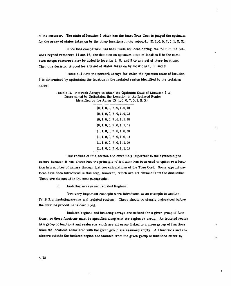
of the restorer. The state of location 5 which has the least True Cost is judged the optimum
for the array of states taken on by the other locations in the network, (X, 1, 0, 0, ?, 0, 1, X, X).
Since this comparison has been made not considering the form of the net-
work beyond restorers 11 and 16, the decision on optimum state of location 5 is the same
even though restorers may be added to location 1, 8, and 9 or any set of these locations.
Then this decision is good for any set of states taken on by locations 1, 8, and 9.
Table 4-4 lists the network arrays for which the optimum state of location
5 is determined by optimizing the location in the isolated region identified by the isolating
array.
Table 4-4. Network Arrays in which the Optimum State of Location 5 isDetermined by Optimizing the Location in the Isolated Region
Identified by the Array (X, 1, 0, 0, ?, 0, 1, X, X)
(0, 1, 0, 0, ?, 0, 1, 0,0)
(0, 1,0,0, ?, 0, 1, 0, 1)
(0, 1, 0, 0, 0, 1, 1, 0)
(0, 1,0,0, ?, ,1, 1, 1)(1, 1, 0, 0, ? 0, 1,0, 0)
(1, 1, 0, 0,?, 0, 1, 0, 1)
(1,1,0,0,?, 0,1,1,0)
(1, 1,0,0, ?, ,1, 1, 1)
The results of this section are extremely important to the synthesis pro-
cedure because it has shown how the principle of isolation has been used to optimize a loca-
tion in a number of arrays through just two calculations of the True Cost. Some approxima-
tions have been introduced in this step, however, which are not obvious from the discussion.
These are discussed in the next paragraphs.
d. Isolating Arrays and Isolated Regions
Two very important concepts were introduced as an example in section
IV. B. 2. a.; isolating arrays and isolated regions. These should be clearly understood before
the detailed procedure is described.
Isolated regions and isolating arrays are defined for a given group of func-
tions, so these functions must be specified along with the region or array. An isolated region
is a group of functions and restorers which are all error linked to a given group of functions
when the locations associated with the given group are assumed empty. All functions and re-
storers outside the isolated region are isolated from the given group of functions either by
4-12

restorers or by the form of the network. Any set of functions and restorers which fulfills
this requirement is an isolated region. The restriction that the locations of the given group
of functions be empty is only necessary for defining the region. During the procedure, these
locations will take on various states.
For each isolated region there is one and only one isolating array which,
together with the identity of the given group of functions, completely defines the isolated
region. The array specifies as 1 the locations at the boundaries of the region in which re-
storers are required to isolate functions outside the region from the given group of functions.
Also specified as either 1 or 0, are all the locations within the isolated region. The states of
the locations of the given group of functions or the locations not necessary to define the region
are not specified in the isolating array. Only locations required to identify the members of
an isolated region are specified in the isolating array.
3. The Approximations in the Procedure
a. The Quantity Minimized
The Isolating Array Synthesis Procedure does not find the network which
minimizes the True Cost of equation 4. The technique uses an approximation of this cost,
so that the characteristic of isolation can be used to considerably reduce the number of cal-
culations that must be performed in the optimization procedure.
Assume a set of functions are chosen from the network and called mem-
bers of the set Q. The locations of the set Q are to be optimized, but fur the moment let the
locations of every member of the set Q be empty. Now let the locations of the functions not
in the set Q take on an array of states with some locations filled and some empty.
The functions and restorers not in Q can be divided into two sets, E and I.
A member of set E is error-linked to at least one of the members of set Q and a member of
set I is isolated from every member of Q. Three disjoint sets have now been defined.
The approximation is based on the method of computing the reliability of
redundant networks which is described in detail in Appendix A. This appendix shows that the
reliability of a network, R, can be factored into two terms RI and RE such that:
R = RIRE.
R, consists only of factors which contain the reliabilities of circuits in
functions in the set I, outside the isolated region. RE consists only of factors which contain
the reliabilities of circuits in functions in the sets E and Q, inside the isolated regions.
4-13

Now say the states of the locations within the set Q are to be optimized, with
the locations not in set Q specified as some array. When a restorer is placed in a location,
it takes on the function's outputs. The functions and restorers that were error-linked to the
function alone are now error-linked to the function or its restorer or perhaps both, but no
new functions are error-linked with the combination. Then, as restorers are added to the set
Q, the sets I and E remain the same. No new terms are introduced into R, , so it does not
change, but RE changes because of changes in the set Q.
The optimum array of the states of the locations in the set Q (given the ar-
ray of the locations not in Q) is that which minimizes the True Cost. The functional costs of
the sets Q, I, and E are independent and are represented by FQ, FI, and FE respectively.
The True Cost for this network is written:
True Cost = FI + F E + FQ + (1 - RIRE) K. (5)
Since only the members of set Q are allowed to change, only the terms FQ
and RE of the True Cost will vary. Say there are two different arrays of the locations in
Q, Q' and Q", whose True Costs are being compared. The difference between the cost of the
two networks is:
True Cost (Q') - True Cost (Q") = FQ(Q') - FQ(Q")
+ 1-RIRE(Q')] K - [I-RIRE(Q"]) K
FQ(Q') - FQ(Q") + RI [RE(Q") - RE(Q')] K
(6)
For most situations, the value of RI will be very close to 1 and will have
very little effect on the decision between the arrays Q' and Q". Then the approximate dif-
ference between the true costs of the two arrays is:
True Cost (Q') - True Cost (Q") i FQ(Q') - FQ(Q")
+ [RE(Q")- RE(Q')] K. (7)
The optimum array of the locations in set Q found using this equation is in-
dependent of the functions or restorers in the set I. The equation affirms that the optimum
state of a set of locations does not depend on the functions or the state of the locations that
are isolated from the functions in the set. This is a very important approximation and it is
4-14

the crux of the Isolating Array Synthesis Procedure. Its use considerably reduces the num-
ber of calculations the designer will have to make for the synthesis of a large multiple-line
network as shown in the last section.
In the procedure, the only costs calculated are the costs of the isolated
regions made up of the sets Q and E. This cost is called the region cost and is:
p (Q') = FQ(Q') + FE + [1-RE(Q')] K (8)
The region cost is independent of the set I. The difference between region
costs for the arrays Q' and Q" results in equation 7.
b. Calculation of the Region Cost
The region cost is described by equation 8. In this study, the region cost
has been calculated with an approximation which simplifies its determination and quickens the
accomplishment of the synthesis procedure.
A region is made up of one or more indivisible isolated regions. An indi-
visible isolated region is one in which every function within the region is error-linked with
some other function in the region and every function outside the region is isolated from all
the functions inside. An example of a network containing two indivisible isolated regions is
shown in figure 4-3.
Figure 4-3. Network Containing Two Indivisible Isolated Regions
Functions 1, 2, and 3 form one indivisible isolated region; and restorer 9
and functions 4, 5, and 6 form the other.
Since individual isolated regions contain no functions in common, the cost
and reliability of one is independent of the cost or reliability of any other.
Thentthe cost of indivisible isolated region 6 is written:
=F + (1 -IRe) K (9)
If a region is made up of a number of indivisible regions, its costs is
written:
allG
4= -(10)
i 4-15

This is an approximation to the region cost of equation 8. It is valid if the
reliabilities of the individual indivisible isolated regions are high.
c. The Effect of the Approximations on the Optimum
Parts a. and b. of this section have noted the approximations to the True
Cost that have been made for this study. In almost all cases, they will not seriously effect
the results of the synthesis procedure. If the result is different from the True Optimum, the
cost of the resulting network will probably not be much greater than the minimum True Cost.
Both approximations assume that the optimization of a small isolated region,
independent of the rest of the network, is consistent with the optimization of the whole net-
work. The approximations essentially optimize a region, assuming the rest of the network is
perfectly reliable. The difficulty is that the actual cost of failure of the isolated region is
dependent on the reliabilities and location states outside the region. For example, consider the ex-
treme case where the reliability of circuits in a function outside the isolated region is zero.
These circuits cannot operate correctly, and the network is surely failed. A restorer added
to minimize the cost of a region is really no help at all to the total network, since it has al-
ready failed. The restorer can only add to the functional cost of the network. The procedure
does not take into consideration functions outside the isolated region, so the result of the pro-
cedure in this case may not be optimum.
This extreme example has turned up the approximation in the procedure, but
this is not serious. A good portion of the network need not be considered when determining
the optimum state of a location. This proves to be so valuable an attribute that it far out-
weighs the approximation brought to light in this section.
It does only lead to a slight approximation, because almost all networks that
will be synthesized will have extremely high reliability specifications. When optimizing a
location, using some small portion of the network, it is not very erroneous to assume that
the rest of the network is working. Under this assumption, the procedure as described so
far is perfectly valid.
When K, the cost of failure, is so high that the goal of the design is to maxi-
mize the reliability of the network, the procedure is valid without any approximation. No
matter what the reliabilities of the functions outside the region which includes function 5 in
the example, the optimum state of location 5 is the one which minimizes the probability of
failure of the region and therefore, minimizes the expected cost of failure of the region. Uti-
lizing the optimum cannot decrease the reliability of the network, and it will increase it if the
rest of the network is not sure to fail.
4-16

4. The Detailed Procedure
a. Example Network
This section presents the detailed description of the synthesis procedure
with an example to illustrate its principles. The example is continued throughout the dis-
cussion.
The example network is shown in figure 4-4, with the stated characteristics.
Reliability of a circuit in each
function = .99
Reliability of a restoring cir-
cuit = .999
Functional cost of a circuit
in a function = 10
Functional cost of a restoring
circuit = 20
Cost of Failure K = i06
m= 5*
k = 3*
* m and k defined in Section M. A.
Figure 4-4. Example Network for the Detailed Procedure
The first step in the procedure is to number the functions of the network.
Numbers may be assigned in any manner with one restriction. A function designated Z must
be a primary source or a primary sink of a function designated with a number less than Z.
This is always possible. There may be an optimum way to designate the functions of the net-
work, but this has not been determined.
The functions of the example are numbered in figure 4-5.2 3 4
Figure 4-5. Example Network with the Functions Identified
4-17

The second step of the procedure is a listing of the isolating arrays of the
first function. A technique for determining these arrays appear in Appendix B.
The state of all locations of functions that are at the output of the network
and do not form inputs to functions in the network are set equal to 0 in all arrays. These
functions are assumed restored in Section III. A. 3. d.; hence, there can be no increase in
reliability or decrease in functional cost brought about by including restorers in their loca-
tions. Their locations will remain 0 throughout the synthesis procedure.
The isolating arrays of function 1 of the example are listed in Table 4-5.
The derivation of this list is shown in Appendix B. Function 4 forms an output and is a
source of no other functions in the network, so its location assumes the state 0 in each array.
Table 4-5. Isolating Arrays of Location 1
1 ? 1X01X
2 ?11001
3 ? 0101X
4 ?01001
5 ?11000
6 ?10001
7 ? 10000
8 ? 00011
9 ?00010
10 ? 0 0 0 0 1
11 ? 0 1 0 0 0
12 ? 0 0 0 0 0
The process for optimization begins with the determination of the optimumstate of the first location for each of its isolating arrays. The procedure is begun by finding
the isolated region which is described by the first isolating array of the first location. Theisolated region is defined by the array and the requirement that all functions be error-linked
with the first function when the first location is empty. The technique for finding the form of
the isolated region from the isolating array will be described in Appendix C.
The cost of this region is now computed under two states; first, with a re-
storer in location 1 and, second, without a restorer in this location. These two costs are
compared, andthe less expensive of the two designs is retained while the more expensive
is discarded. The optimum state of location 1 for the given isolating array now has been de-
termined.
4-18

When comparing the cost of two alternatives, it is important that the regions
of both alternatives include the same functions. To assure this, the isolated region should be
constructed with the location being optimized empty. The, using the same region, the loca-
tion should be filled and the costs of the alternatives compared.
A sample of isolating array is selected for an example, (?, 1, X, 0, 1, X).
Its isolated region is generated and shown in figure 4-6.
Figure 4-6. The Isolated Region of the Isolating Array ofthe First Function ( ?, 1, X, 0, 1, X)
Location 1 is assigned its two possible states. The regions for the two
states, divided into indivisible isolated regions, appear in figure 4-7.
Arrays Regions
1) (0, 1, X, 0, 1, X) 2
2) (1,1,X,0,1,X)
Figure 4-7. The Isolated Region of Figure 4-6 with Location 1taking on its two Possible States
For this example, with location 1 empty, array 1 of figure 4-7 describes
an indivisible isolated region consisting of functions 1, 2, and 5. With location 1 filled,
array 2 describes a region with two indivisible isolated regions, one consisting of function 1
alone and the other consisting of functions 2, 5, and restorer 7. According to Section IV. B.
3. b., the costs of these two indivisible regions are added to find the cost of the region of
array 2.
To find the optimum state of location 1 for this isolating array, one needs
only compare the region costs of the regions defined by arrays 1 and 2. The results of the
optimization hold for all states taken on by the X coordinates in the isolating array. For
4-19

this example, the region cost of the region for array 1 is 299, for array 2 is 286. Therefore,
for the isolating array (?, 1, X, 0, 1, X) the optimum state of location I is to have a restorer
present.
The cost of the region in which location 1 takes on its optimum state, array
2, is retained for use later in the procedure. This region will appear again as other loca-
tions are optimized.
What does the discovery of the optimum state of location for an isolating
array contribute toward the accomplishment of the synthesis procedure? The optimum state
of the location does not depend on the locations that are not specified in the array. Then the
decision on the state of location 1 determines two sets of network designs which are com-
pletely specified as the X'd locations take on values. One set consists of network designs
which may be optimum, and the other consists of designs that cannot be optimum. The latter
set can be discarded, as each member is more expensive than some member of the former
set. This is accomplished by only retaining the state of location 1, which resulted in the
cheapest isolated region for the given array.
For the example, the two sets are shown in table 4-6.
Table 4-6. Two Sets of Designs that are Generated by the Optimization ofLocation 1 for the Isolating Array (?, 1, X, 0, 1, X)
Designs which Designs whichmay be optimum cannot be optimum
(1, 1,0, 0, 1,0) (0, 1,0,0, 1,0)
(1, 1,0, 0,1, 1) (0,1,0,0,1,1)
(1, 1,1, 0,1, 0) (0, 1,1,0, 1,0)
(1,1,1,0,1,1) (0,1,1,0,1,1)
The difference in the two columns is the value of x1. The designs in the
right hand column cannot be optimum since by changing the state of location number 1 to 1,
the cost will be reduced. The optimum is not necessarily one of the designs in the left hand
column, but it may be.
The gain achieved by this first step in the technique is that four network
designs have been eliminated from consideration by two cost calculations. This is twice as
effective as the exhaustive search routine in which each calculation eliminates one alternative.
The gain arises because the decision was made without regard to the states
of locations 3 and 6, and since the regions are independent, the decision is good for all states
of 3 and 6.
4-20

This process is then repeated for all the remaining isolating arrays of
location 1. The results yield the optimum states of location 1 for all its possible isolating
arrays. For each isolating array, the calculations will eliminate one or more design alterna-
tives. It should be noted that the more locations that remain unspecified by the isolating ar-
ray (X's in the vector), the more effective the calculations will be in eliminating alternatives.
The isolating array which specifies all locations except the first location only eliminates one
alternative. When all the isolating arrays about the first location have been considered, the
procedure will have determined the optimum state of the first location for any possible array
of the other locations in the network. For each array there are two alternatives for the first
location, and one of these will be eliminated. When the calculation has been made for all
possible isolating arrays, one half of the 2s alternative designs will have been eliminated.
That is, 2s - 1 alternatives will have been determined as not possibly optimum, leaving 2 - 1
alternatives from which the optimum is to be chosen.
The number of calculations required to accomplish this step of the synthesis
procedure depends on the number of isolating arrays of the first location. This, of course,
depends in turn on the interconnections between the functions of the networks. In almost all
networks, it will be far fewer than the 2s - 1 calculations required by the exhaustive search
routine.
For the example, the optimum state of location 1 has been determined for
each of its isolating arrays. The results of the optimization, together with the cost of each
optimum configuration, is tabulated in table 4-7.
Table 4-7. The Optimum State of Location 1 and the Cost of the OptimumIsolated Region for each Isolating Array of Function I
Isolating arrays of Optimum state of Cost of optimumlocation 1 location 1 configuration
1 (? 1X01X) 1 286
2 (?11001) 1 659
3 (?0101X) 1 529
4 (?01001) 1 737
5 (?11000) 1 1044
6 (?10001) 1 1061
7 (?10000) 1 12638 (?00011) 1 982
9 (? 00010, 1 1263
10 (?00001) 1 1329
11 (? 01000) 1 1122
12 (? 00000) 1 1735
4-21
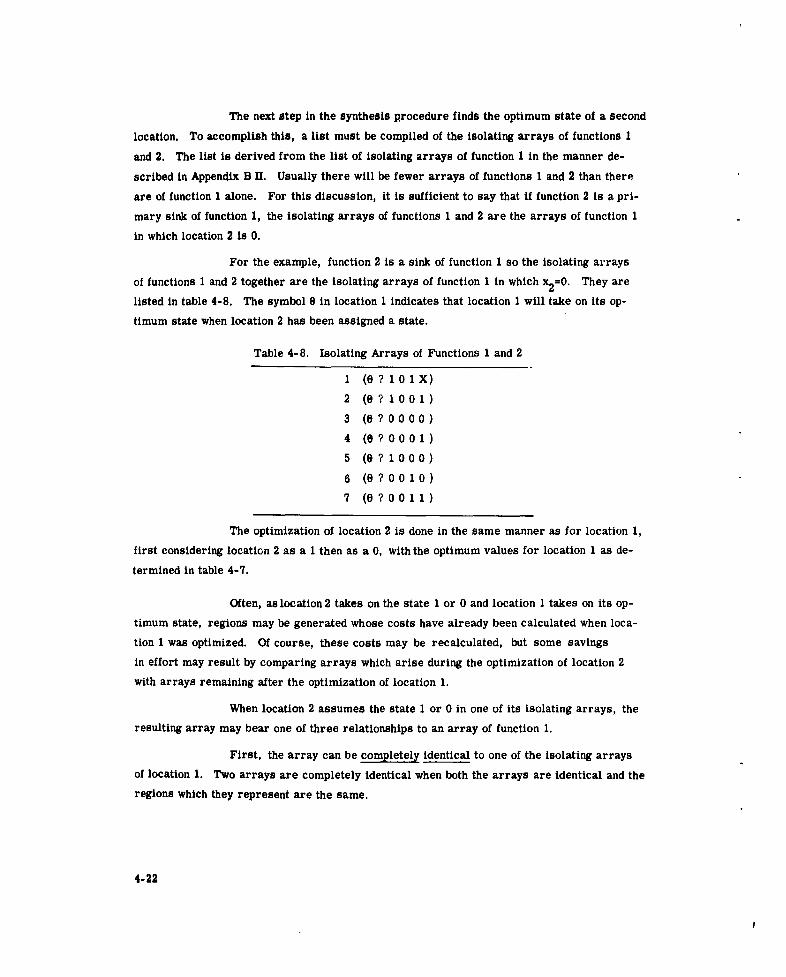
The next step in the synthesis procedure finds the optimum state of a second
location. To accomplish this, a list must be compiled of the isolating arrays of functions 1
and 2. The list is derived from the list of isolating arrays of function 1 in the manner de-
scribed in Appendix B II. Usually there will be fewer arrays of functions 1 and 2 than there
are of function 1 alone. For this discussion, it is sufficient to say that if function 2 is a pri-
mary sink of function 1, the isolating arrays of functions 1 and 2 are the arrays of function 1
in which location 2 is 0.
For the example, function 2 is a sink of function 1 so the isolating arrays
of functions 1 and 2 together are the isolating arrays of function 1 in which x2=0. They are
listed in table 4-8. The symbol 9 in location 1 indicates that location 1 will take on its op-
timum state when location 2 has been assigned a state.
Table 4-8. Isolating Arrays of Functions 1 and 2
1 (6? 101X)
2 (8?1001)
3 (e?0000)
4 (8?0001)
5 (9?1000)
6 (E?0010)7 (670011)
The optimization of location 2 is done in the same manner as for location 1,
first considering location 2 as a 1 then as a 0, with the optimum values for location 1 as de-
termined in table 4-7.
Often, as location 2 takes on the state 1 or 0 and location 1 takes on its op-
timum state, regions may be generated whose costs have already been calculated when loca-
tion 1 was optimized. Of course, these costs may be recalculated, but some savings
in effort may result by comparing arrays which arise during the optimization of location 2
with arrays remaining after the optimization of location 1.
When location 2 assumes the state 1 or 0 in one of its isolating arrays, the
resulting array may bear one of three relationships to an array of function 1.
First, the array can be completely identical to one of the isolating arrays
of location 1. Two arrays are completely identical when both the arrays are identical and the
regions which they represent are the same.
4-22

When an isolating array of locations 1 and 2 with function 2 taking some
state is completely identical to an array already calculated for location 1, the cost will be the
same and does not have to be recalculated.
If both arrays (a 1 and a 0 in location 2) are completely identical to arrays
which have been calculated for location 1, no further calculations need be made - a simple
comparison of costs will produce the optimum state of location 2, and hence, of the first
two locations.
Second, the array can be incompletely identical to one of the isolating ar-
rays of location 1. They are incompletely identical when the arrays are identical, but the
regions which they represent differ from each other.
The isolated region of functions 1 and 2 is now defined by an array and the
requirement that all functions are error-linked to either function 1 or 2 when locations 1 and
2 are empty. For a particular array, functions which are error-linked to function 2 but not
function 1 will be included in the isolated region of functions 1 and 2, but not in the region of
function 1 alone. Instances such as this give rise to incompletely identical arrays.
It must be remembered that the costs of regions represented by incompletely
identical arrays are not the same. The cost of such a region must be recalculated.
Third, the array can be not identical to any of the isolating arrays of loca-
tion 1. They are not identical when the arrays themselves differ. Of course, if an array is
not identical to any arrays formerly generated, the cost of its region must be determined.
Comparing the isolating arrays of functions 1 and 2 with those of function 1
only, it can be seen that array 3 in table 4-8 with a 0 in location 2 is an isolating array of
both function 1 and functions 1 and 2, and is completely identica to array 12 in table 4-7.
Since the two arrays are completely identical, the cost computed in the isolating arrays of
location 1 can be retained and used in determining the optimum state of location 2. With a 1
in location 2, array 3 of table 4-8 is completely identical to array 7 in table 4-7 and its cost
is retained. The costs of the two regions are now compared, andtheless expensive describes
the optimum state of locations 1 and 2 for this isolating array, (i. e, in table 4-7, array 7
costs 1263 and array 12 costs 1735).
Isolating array 7 (of functions 1 and 2) with a 1 in location 2 is not identical
to any isolating array of location 1 and requires complete calculation of cost, while the same
isolating array with a 0 in location 2 is completely identical to isolating array 8 of function 1;
hence, the cost of array 8 of function 1 can be used as the cost for array 7 of functions 1 and
2 with a 0 in location 2. The comparison shows that isolating array 7, with a 1 in location 2
4-23

is the cheaper of the two (870 vs 982) and is therefore retained. The optimum state of loca-
tion 2 for this isolating array is to have a restorer present. The optimum state of location
1, has already been determined, and it too should be filled. For this array, both locations
should be filled for minimum cost.
Table 4-9 lists this result with the optimum state of locations of 1 and 2 for
each array.
Table 4-9. The Optimum State of Locations 1 and 2 and the Cost ofthe Optimum Isolated Region for each Isolating Array
of Functions 1 and 2
Isolating arrays of Optimum states of Cost of optimumlocation 1 and 2 locations 1 and 2 configuration
1 (0, ?, 1,0, 1,X) 1,0 529
2 (, ?, 1,0,0, 1 ) 1,1 659
3 (0, ,0,0,0,0) 1,1 1263
4 (O,?,0,0,0,1) 1,1 1061
5 (0,?,1,0,0,0) 1,1 1044
6 (e, ?,00, 1, ) 1,0 1263
7 (, .,0,0,1, ) 1,1 870
In this step of the procedure, the state of location 2 has been optimized
using the optimum state of location 1. During the performance of this step, half of alterna-
tive networks remaining after the optimization of the first location have been eliminated from
consideration.
The Synthesis Procedure continues in a similar manner. The isolating
arrays of functions 1, 2, and 3 are found. If 3 is a primary sink of functions 1 or 2, its iso-
lating arrays are the same as the arrays of functions 1 and 2 in which x 3=0. If function 3 is
a primary source of one of the functions and not a primary sink, some new arrays may have
to be generated.
For each of the isolating arrays, let the third location take on the states 1
and 0. The optimum states for the first two locations have already been determined in the
previous steps for each choice of the state of location 3 for each isolating array. Further-
more, the cost of the alternative with x3 =0 has been determined in the second step if the
array is a complete identity to one of the isolating arrays of functions 1 and 2. There may
be only one calculation to make, then, for an isolating array and that may be the region cost
with x3 =1, and x and x2 having the optimum states as determined in the previous step. The
4-24
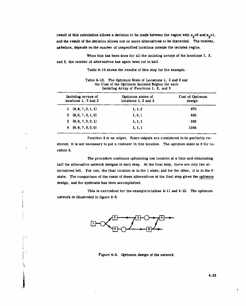
result of this calculation allows a decision to be made between the region with x3 =0 and x3 =1,
and the result of the decision allows one or more alternatives to be discarded. The number,
as before, depends on the number of unspecified locations outside the isolated region.
When this has been done for all the isolating arrays of the functions 1, 2,
and 3, the number of alternatives has again been cut in half.
Table 4-10 shows the results of this step for the example.
Table 4-10. The Optimum State of Locations 1, 2 and 3 andthe Cost of the Optimum Isolated Region for each
Isolating Array of Functions 1, 2, and 3
Isolating arrays of Optimum states of Cost of Optimumlocations 1, 2 and 3 locations 1, 2 and 3 design
1 (0,,?,0, 1,1) 1,1,0 870
2 (0,0, ?,0,1,0) 1,0,1 836
3 (0,0, ?0, 0, 1) 1,1,1 926
4 (0,0, ,0,0, 0) 1,1,1 1044
Function 4 is an output. Since outputs are considered to be perfectly re-
stored, it is not necessary to put a restorer in this location. The optimum state is 0 for lo-
cation 4.
The procedure continues optimizing one location at a time and eliminating
half the alternative network designs at each step. At the final step, there are only two al-
ternatives left. For one, the final location is in the 1 state; and for the other, it is in the 0
state. The comparison of the costs of these alternatives at the final step gives the optimum
design, and the synthesis has been accomplished.
This is carriedout for the example in tables 4-11 and 4-12. The optimum
network is illustrated in figure 4-8.
Figure 4-8. Optimum design of the network
4-25

Table 4-11. Optimization of Location 5
Isolating arrays of Optimum states of Cost of Optimumlocations 1, 2, 3, 4, 5 locations 1, 2, 3, 4, 5 design
1 (, e, ,0, ?, 1) 1,1,0,0,1 870
2 (e,e,e,0, ?,0) 1,0,1,0,1 836
Table 4-12. Optimization of Location 6
Isolating arrays of Optimum states of Cost of Optimumlocations 1, 2, 3, 4, 5, 6 locations 1, 2, 3, 4, 5, 6 design
1 (e,e,e,o,e, ?) 1,0,1,0,1,0 836
D. SOME EXAMPLE RESULTS OF THE PROCEDURE
An example network has been optimized under several conditions of reliability, func-
tional and failure costs. This network is a seven stage shift register of order 5 redundancy.
The results of this optimization technique are contained in table 4-13. For comparison, the
costs and reliabilities of the non-redundant case are listed also.
For this example, the synthesis procedure was carried out by hand with the help of a
computer to determine the reliabilities or alternative regions. The program for determining
the reliabilities of multiple-line networks is described in Section X of Appendix A.
In most cases, when the cost of failure is an important factor, the optimum 5th order
redundant network is cheaper than the non-redundant case. This is due to the fact that the
cost of adding more circuits to the network is not as important as the savings in keeping the
network from failing.
In cases 2, 8, 9, and 10, there are three optimum configurations. These networks
all have the same network cost.
In cases 6 and 9, the non-redundant cost is not as great as that for the optimum 5th
order redundant network. These cases result from the assignment of high costs to the addi-
tion of functions, the low cost of failure or a combination of these. In these cases, the dif-
ference in functional cost between the non-redundant case and the 5th order redundant case
is significant compared to the cost saving in improved reliability. Since the number of cir-
cuits necessary for a given case is a very real consideration in these calculations, the
cheapest network is also a function of this number. The optimum configuration listed in the
table is the optimum 5th order system. It may well be that the optimum network with order
4-26

cc 0i i i i ii i i~ IS
I S,, ,.a a
N Mi -i i-i- - - -
-,, , WI W ,,'I
-0 I
6
6' 'Y 6 6I iI i[ I I il IJJ:1:IE : :I I P ,il I04 ~ ~ W 0 Id d P
1.
- ~ 0 N~ 0 0 0 0 0 Ccc to to M2 to M1 (D
N010 D dO D -II -I WI W I I I - ID
e COM cc a00
- - - - -II--
I.
is a
0 . .. .0 * . ... .- I'
Table 4-13. Example Results of the Optimization Technique
4-27

3 redundancy, would be the cheapest since savings are made over the functional cost of the 5th
order as well as savings in failure cost over the non-redundant case.
In order to arrive at the optimum order of redundancy it would be necessary to deter-
mine the optimum configuration for each order of redundancy; then compare the costs. The
cost comparison between the costs of the different optimum networks should produce the
cheapest network design.
4-28

V. CONCLUSIONS AND RESULTS
This study has evolved the Isolating Array Synthesis Procedure to aid in the design of
redundant multiple-line networks. The procedure is applicable to networks of general topo-
logy, but the order of redundancy of all the network's functions are required to be the same.
The several steps of the procedure have been developed in sufficient detail so that small
example networks have been synthesized and the procedure is ready for computer implemen-
tation.
The practicality of this technique, as far as the number of operations required to per-
form synthesis is concerned, has not been established. However, the procedure should
have considerable advantages over the exhaustive search technique for large networks where
the problem of synthesis is most acute. The maximum number of isolating arrays of a func-
tion arises when the function is directly connected to every other function in the network.
This maximum number is the same as the number of all possible network arrays which is the
number of calculations one must perform in the exhaustive search procedure. Then, if each
function of the network is directly connected to every other function, the Isolating Array Syn-
thesis Procedure offers no improvement over the exhaustive search technique.
The minimum number of isolating arrays of a function occurs when the functions are
connected as a shift register with no feedback. Each function feeds not more than one other
function and receives its inputs from no more than one function. This number is far less
than the number of calculations for the exhaustive search procedure. A real network will
fall somewhere between these extremes with each function directly connected to only a few
others. Then the number of isolating arrays of a function, hence the number of calculations
one has to perform in the accomplishment of the procedure will be an extremely small frac-
tion of those required by exhaustive search techniques. Because of their size, the examples
shown in this report do not illustrate this advantage of the procedure. Full evaluation of the
procedure will require further study.
The criterion chosen for optimization reflects the author's view of the factors that
might be important in applications where redundancy will be used. The procedure does not
depend on the choice of these factors; hence, they are amenable to change.
The procedure does not give the true optimum when the costs of implementation, weight
and power are considered, but the approximation is small when the reliability of the circuits
of the network is high. It is likely that the True Cost of the result of the procedure is very
5-1
little greater than the minimum True Cost. When the only goal of the designer is to maxi-
mize the reliability of the network, the Isolating Array Synthesis Procedure does yield the
truly optimum network design.
The work done to this point represents only a first step in the evolution of the synthesis
procedure; it still remains to remove the restriction that the order of redundancy be constant
throughout the network. It is a very important step however, in that It performs an optimi-
zation never before achieved. The procedures when fully developed may be applicable to
other optimization problems.
As a necessary part of the synthesis procedure, a reliability analysis procedure de-
scribed in Appendix A, has been developed. This procedure has significant advantages over
otaer attempts to determine the reliability of multiple-line networks in that it is applicable
to networks of general form. There are no restrictions on the interconnection between func-
tions of the network and, few restrictions on the character of the component circuits. One
restriction that the circuit have only one output will soon be removed by a study now in pro-
gress. The order of redundancy of functions is a variable in the reliability analysis tech-
nique, and under certain conditions different portions of the network may have different
orders of redundancy.
The procedures developed in this study will give the designer a tool with which he can
design a multiple-line network confident in the knowledge that he is using the redundancy to
full advantage. This tool is not presently available. This is necessary because the effective-
ness of redundancy in increasing reliability varies greatly with the manner in which it is ap-
plied. A misplaced restorer or too great an order of redundancy may actually be detrimental
to a network's reliability.
Work yet to be performed includes further study of the synthesis procedure to deter-
mine if the number of calculations required can be reduced. A full evaluation of the proce-
dure is necessary to find if, through its use, synthesis can be accomplished in a reasonable
amount of time. To use the procedure on a large network, computer implementation will be
necessary; a program will be prepared to this end. When the program is available, a num-
ber of examples will be tried to generate some "rules of thumb" which may be used in design
more easily than the procedure. Future studies will attempt to remove the restriction that
the network have a constant order or redundancy.
5-2

TABLE OF CONTENTS
Section Pg
I RELIABILITY APPROXIMATIONS FOR THE REDUNDANT NETWORK. A-3
U IDENTIFYING THE MINIMAL CUTS OF THE GENERAL MULTIPLE-LINE NETWORK. .. ...... .......... ........ A-9
inl IDENTIFYING THE MINIMAL PATHS OF THE GENERALMULTIPLE-LINE NETWORK. .. .......... ........ A-13
IV MATRIX TECHNIQUES. .. ........ ........... .. A-19
A. Definitions of Terms .. ..... .......... ....... A-19
1. Boolean Matrix. .... ........... ........ A-19
2. Primary Matrix .. ..... ........... ..... A-20
3. Secondary Matrix. .... ........... ....... A-22
4. nth Order Matrix. ..... ........... ..... A-23
5. Composite Matrix. ... .......... ......... A-23
6. Error-Linked Source Matrix .. .. ....... ........ A-24
B. Determination of the Composite Matrix. .. ....... ..... A-25
V DETERMINING THE MINIMAL CUTS OF A NETWORK FROMITS ERROR-LINKED SOURCE MATRIX. .. ..... ......... A- 27
A. Order Three Redundant Network .. .. ........... ... A- 27
B. General Multiple Line Networks. .. ........ ........ A- 29
C. Different Orders of Redundancy. .. .......... ..... A-32
VI DETERMINATION OF THE MINIMAL PATHS OF A NETWORKFROM ITS ERROR-LINKED SOURCE MATRIX. .. ... ........ A-33
VII DETERMINING RELIABILITY WHERE ONE FUNCTION IS AN ERROR-LINKED SOURCE OF TWO OTHERS OF DIFFERENT ORDERS OFREDUNDANCY .. ......... ........... .... A-35
A. First Kind of Cuts .. ..... .......... ........ A-35
B. Second and Higher Kinds of Cuts .. .. ........... ... A-38
1. Second and Higher Kinds of Cuts Between Functionsof Set Q, R, or Qand R. .. ........ ......... A-39
a. Second Kind of Cuts for Functions in Set Q .. ... ..... A-40
b. Second Kind of Cuts for Functions in Set R. ... ..... A-40
c. Second Kind of Cuts for Set Q and R .. ....... ... A-40
d. General Expression for Second and Higher Kindof Cuts in Set Q, R, or QandR .. ..... ....... A-41
2. Second and Higher Kinds of Cuts In Sets Q2, S, or Q2and S. ........ .......... ........ A-43
C. Reliability Due to Second and Higher Kinds of Cuts .. .. ....... A-44
D. Total Reliability. .. ....... ........... .... A-45
A-i

TABLE OF CONTENTS (Continued)
Section Page
VIII DETERMINING RELIABILITY WHERE ONE FUNCTION IS AN ERROR-LINKED SOURCE OF ANOTHER WHICH IS OF HIGHER ORDER OFREDUNDANCY ........ ......................... .... A-47
IX SINGLE LINE RESTORER ANALYSIS ........ ................ A-51X PROGRAM FOR COMPUTING THE RELIABILITY OF A REDUNDANT
SYSTEMS ............ ........................... A-53
A. Generating the Error-Linked Sotirce Matrix ............. .... A-53B. Calculating the Reliability of a System .... .............. ... A-54
1. Identifying the Minimal Cuts ..... ................ .... A-55a. First Kind of Minimal Cuts .... .............. .... A-55
b. Second Kind of Minimal Cuts ....... .............. A-55
c. Third and Higher Kinds of Cuts ...... ............. A-55
2. Computation of Reliability ..... ................. ... A-56
LIST OF ILLUSTRATIONS
Figure e
A-1 Restoration Between Different Orders of Redundancy ........... ... A-1
A-2 Example Network for the Reliability Analysis ... ............ .... A-2
A-3 Example of a Coherent Network ...... .................. .... A-5A-4 The Partial Networks of the Example Network ... ............ .... A- 13
A-5 General Matrix ........ .......................... .... A-19A-6 Flow Graph and Primary Matrix for a Redundant Network .......... A-21
A-7 The Secondary Matrices of the Example Networks of Figure A-6. . .. A-23
A-8 The Error-Linked Source Matrices of the Example Networkwith a) no restorer; b) restorers after functions 2 and 5 ... ...... A-24
A-9 Error-Linked Source Matrix for the Network of Figure A-2 ......... A-27
A-10 A Function which is an Error-Linked Source for Two Functionswith Different Orders of Redundancy .... ............... .... A-36
A-11 The First Example Showing a Function of Order 5 RedundancyProviding the Inputs to a Function of Order 7 Redundancy ......... A-48
A-12 Example Showing a Function of Order 5 Redundancy Providingthe Inputs to a Function of Order 7 Redundancy ............. .... A-49
A- 13 Single Line Restorer ........ ....................... .... A-51
A-it

APPENDIX A
DETERMINATION OF THE RELIABILITY OF MULTIPLE LINE NETWORKS
The ability to determine the reliability of redundant networks is a prime requisite to
any synthesis technique. The analysis techniques developed to date and available in the
literature are not sufficiently general for application to real networks. This appendix de-
velops a method for analyzing the reliability of general redundant networks.
The type of redundancy to which this analysis is applicable is described in section III
in the text of the report, hence it can be applied to the problems encountered in the synthesis
procedure. However, it can be used to analyze more general networks than those that can
be handled by the synthesis procedure, because some of the restrictions on the order of
redundancy of the functions in the network have been removed. In the first part of the
appendix different functions are allowed to have different orders of redundancy. The order
of redundancy may change only after passing through a restorer. Functions with different
orders of redundancy cannot be directly interconnected. In a multiple line system, the
number of restoring circuits in the restorer is equal to the order of redundancy of the func-
tions the restorer feeds. Using this rule, figure Al shows how a function of order 5 re-
dundancy is connected to a function of order 3 redundancy through a restorer; "a" shows the
transfer from the higher order to the lower order and, "b" shows the transfer from the
lower order to the higher order. In Sections I - VI of this Appendix, it is assumed that all
the functions which a restorer feeds have the same order of redundancy.
Figure A-1. Restoration between different orders of redundancy;a) Going from order 5 redundancy to order 3,b) Going from 3 to 5
A-1

Even these restrictions on the order of redundancy are tempered in Sections VII and
VIII in this Appendix in which the analysis of certain special cases of the combinations of
different orders of redundancy is performed. These sections show that one should be able to
derive equations which can analyze a network of any particular design no matter how the
orders of redundancy of its functions may vary.
In Section IX of this appendix, the procedure is modified to handle restorers which con-
sist of only one restoring circuit, the single line restorer. Section X describes the imple-
mentation of the reliability analysis procedure using an electronic computer.
The example used to illustrate the concepts of the reliability analysis procedure is
shown in figure A-2. It will be relerredto throughout the discussion.
Figure A-2. Example Network for the Rallability.Analyals
A-2

I. RELIABILITY APPROXIMATIONS FOR THE REDUNDANT NETWORK
The definition of network reliability, taken for this report, is the probability that the
network is successful at time t, given that all its circuits were successful at time zero and
that there is no repair. The reliability of the ith circuit in the network is symbolized by
Pl and is the probability that the circuit is successful at time t given that it was successful
at time zero and that it was not repaired. Time is implicit in the term pi which is a variable
in the analysis to follow. The report assumes that the reliabilities of the circuits in the
network are independent.
The exact reliability analysis of the redundant network is a difficult process which is
not easily applied to general networks. This report gives two approximations to reliability
which are upper and lower bounds, and which are very much easier to determine. The2, 3approximations are based on techniques developed by Proschan and Esary
No exact error analysis has been performed to determine the closeness of these bounds
to the actual reliability of multiple line networks. Sample calculations have indicated that
the lower bound is a very good approximation to the true reliability during early time when
the value of the pi's are close to unity. The upper bound is a very good approximation after
a long period of operation when the Pi's are low. The most important period to the designer
will probably be the early life of the network, the high reliability period, so the lower bound
approximation will find the greatest use. However, with both approximations available,
valid bounds may be found on the network reliability for any time.
Proschan and Esary's analysis is based on the concepts of minimal cuts, minimal
paths, and coherent systems. All these terms refer to the effects of circuit failures on the
operation of the network.
A coherent system is defined by four conditions:
1. If when a group of circuits in the system is failed causing the system to be
failed, the occurrence of any additional failure or failures will not return the
system to a successful condition;
2. If when a group of circuits in the system are successful and the system is
successful, the system will not fail if some of the failed components are
returned to the successful condition;
3. When all the circuits in the system are successful the system will be
successful and,
4. When all the circuits in the system are failed the system is failed.
A-3

If a system fulfills all these conditions, it is a coherent system. The reader will have
little difficulty establishing that the redundant systems described in this report are coherent
systems.
A cut Is a set of circuits such that if they fail the system will have failed regardless
of the condition of the other circuits In the bystem. The system may have a large number
of cuts and a particular circuit may be in more than one of them. An example of a coherent
system is shown in figure A-3. As long as any path through successful circuits exists be-
tween the two terminals of the system, the system Is said to be successful. A circuit failure
opens the path between the two terminals of the circuit.
The cuts of this system are listed in table A-1. The numbers of the circuits describe
the cuts. The failure of any of the cuts will cause the network of figure A-3 to fail.
Table A-1. The Cuts of the Network in Figure A-3
Cut No. Circuits in the Cut
1. 1, 2
2. 1,2, 3
3. 1,2, 4
4. 1,2, 5
5. 1, 2, 3, 4
6. 1, 2, 3, 5
7. 1, 2, 4, 5
8. 1, 2, 3, 4, 5
9. 4, 5
10. 3, 4, 5
11. 2, 4, 5
12. 1, 4, 5
13. 2, 3, 4, 5
14. 1, 3, 4, 5
15. 1, 3, 5
16. 2, 3, 4
A minimal cut is defined as a cut in which there is no subset of circuits whose failure
alone will cause the system to fail. From table A-1 the minimal cuts of the network in
figure A-3 can easily be recognized. They are listed in table A-2 along with their probabili-
ties of occurrence. Since the symbolp 1 represents the probability of success, of the ith
circuit, then (1-Pi) is the probability that the ith circuit fails.
A-4

Figure A-3. Example of a Coherent Network
Table A-2. The Minimal Cuts of the Network in Figure A-3
Min. Cut No. Circuits in the Min. Cut Probability of Failureof the Min. Cut
1. 1, 2 (1-p 1) (1-P2 )
2. 4, 5 (1-p4) (1-p5)3. 1, 3, 5 (1-p 1) (1-P3 ) (1-p 5 )
4. 2, 3, 4 (1-P2) (1-p3) (1-p4)
It is important that the concept of minimal cuts be understood because the lower bound
approximation to reliability depends on the identification of all the minimal cuts in the net-
work. Esary and Proschan found that a lower bound to system reliability is the probability
that none of the system's minimal cuts fail. For the example, this lower bound, RLB is:
RLB = [1-(I-pi) (1-p 2 )] [l- (l-p 4 ) (1-p 5 )] [ (i-p1 ) (l-p 3 ) (1- p5 )]
1 - (l-P 2) (l-P 3) (I-P 4 )]
This relationship can. be written for general systems if the jth minimal cut is denotedby the set S . The members of the Ith minimal cut are given by i e S.. The probability of
failure of the jth minimal cut is:
7r ( i-pi) (A- i)icS.
A-5

The lower bound to the system reliability is the probability that none of the system's
minimal cuts fail or:
RLB = all1i VcS (1 P1 ) (A2)
This is the first approximation this report will use in analyzing redundant systems.
The second approximation deals with the minimal paths of the system. A path is a
set of circuits such that if all the members of the set succeed the system succeeds. The
paths of the example are noted in table A-3.
Table A-3. The Paths of the Network in Figure A-3
Path No. Circuits in path
1. 1, 4
2. 1, 3, 4
3. 1, 2, 4
4. 1, 4, 5
5. 1, 2, 3, 4
6. 1, 3, 4, 5
7. 1, 2, 4, 5
8. 1, 2, 3, 4, 5
9. 2, 5
10. 2, 3, 5
11. 2, 4, 5
12. 1, 2, 5
13. 2, 3, 4, 5
14. 1, 2, 3, 5
15. 1, 3, 5
16. 2, 3, 4
If any one of the sets of components in Table A-3 succeeds, the system will operatecorrectly. A minimal path is defined as a path in which there is no subset of circuits, such
that if all the circuits in the subset succeed alone the network succeeds. The minimal paths
of the network are listed in Table A-4 with the probabilities of success.
A-6

Table A-4. The Minimal Paths of the Network in Figure A-3
Min. Path. No. Circuits in the Min. Path Probability of Successof the Min. Path
1. 1, 4 plp4
2. 2, 5 p2p 5
3. 1, 3, 5 plp3p 5
4. 2, 3, 4 p2P3P4
There is at least one minimal path in each path of the network.
Esary and Proschan showed that for any network an upper bound to the reliability
of the system is the probability that at least one of the minimal paths is successful assuming
that the minimal paths are independent. For the example network this probability, RUB , is:
RUB = 1- (1-plP4 ) ('-IiRp 5) (1-p 1p 3p 5 ) (1-p 2p 3p4 )
In general, if the set of components in the th minimal path is Q. the probability that
this path operates successfuly is:
V i (A-3)
The probability that at least one of the minimal paths of a network succeeds is then:
1- 7r (1- 7r pd (A-4)UB allj ieQ.
This is the upper bound to the reliability of a network that this report uses.
The next step in the analysis of redundant networks is to determine the minimal cuts
and paths of networks in general.
A-7/8

II. IDENTIFYING THE MINIMAL CUTS OF THE GENERAL MULTIPLE-LINE NETWORK
Determination of the lower bound on reliability requires that the minimal cuts of the
network be identified. To accomplish this it first must be clear exactly what constitutes a
network failure.
The state of a network, either failed or successful, is indicated by the state of the
output lines of the restored functions of the network. A restored function either provides
the inputs to a restorer or an output of the network. In either case the output of a restored
function is successful if k of its m output lines are successful. Subject to the restrictions,
on the order of redundancy introduced at the beginning of this Appendix, the values of m and
k may differ for the various restored functions of the network.
An obvious corollary to the above statement is that if less than k output lines are
successful, or more than m-k+1 output lines are failed, the output of the restored function
is failed. When the restored function goes to its restorers, such a condition causes restoring
circuits to make the wrong decision and the output lines of the restorer will all be in error.
Subsequent operations on the signals on these lines cannot correct these errors and the net-
work is failed. When the restored function is a network output, the network is failed by
definition if less than k of its output lines are successful.
A cut then is any group of circuits whose failure causes the outputs of at least one
restored function to have m-k+1 or more failed lines. The problem of this section is to
identify those cuts which fulfill the requirements of minimal cuts outlined in Section I of
the Appendix.
The minimal cuts of a multiple-line redundant network, have three characteristics
which are sufficient to establish their Identity. These are listed below and are followed
by their proofs.
1. All the members of the minimal cut are circuits in a restored function or in
the functions or restorers that are the error-linked sources of that restored
function.
2. The failure of each member of the minimal cut will cause one output line of
the restored function to be in error, and each member will be in a different
position.
3. The failure of a minimal cut will cause exactly m-k+1 output lines of the
restored function to be in error, hence a minimal cut will have m-k+l members.
A-9

Proof of the first characteristic:
Consider a restorer whose outputs are completely in error because of circuit
failures, and assume that this !s caused by the failure of a minimal cut. The restored
function must have m-k+1 or more errors on its output lines. For purposes of this proof
assume that one of the members in the minimal cut is neither in the restored function or in
one of the its error-linked sources. By definition of error-linked sources, the failure of
this circuit will not cause an input line to the restored function to be in error, hence the
errors on the output of the restored function and the failure of the network must be due
entirely to the other members of the cut. Then the failure of a subset of the assumed mini-
mal cut is sufficient to cause failure of the network. This is contrary to the definition of a
minimal cut, and the assumptions made in this proof are incompatible. A minimal cut can-
not include a circuit which is neither in a restored function or in one of its error-linked
sources.
Proof of the second characteristic:
Certainly a failure of a particular circuit in the restored function can only cause
one of the outputs of this function to be in error. The failure of a particular circuit in
error-linked source will disable an input to only one circuit in the restored function. TI n
the failure of each member of a minimal cut will cause one and only one of the output lines
of the restored function to be in error.
To prove that each member of the minimal cut will be in different positions,
assume the contrary and say that there are two members of the minimal cut, a and b, which
are in the same position ana whose failure will affect the same output line of the restored
function. Failure of the minimal cut will disable m-k+1 or more of the output lines of the
restored function. One of these lines is disabled because of the failure of circuits a and b.
But it has been said that failure of a orb alone wiil cause this Ilne tG be in error, so the
failure of all the members except a or all the members except b will still cause failure of
the system. So it is possible to find a subset of the assumed minimal cut (the assumed cut
less a or b) whose failure alone cause system failure. Once again this is contrary to the
definition of a minimal cut, and the assumption that two members of a minimal cut are in
the same position is unjustified.
Proof of the third characteristic:
Any set of m-k+1 erroneous output lines of a restored function is sufficient to
cause the restoring circuits in the restorer to make the wrong decision and the network to be
failed. As established by the first two conditions these errors will be caused by the failure
A-10

of m-k+l circuits in the restored function or in Its error-linked sources. Then any cut
whose failure causes more than m-k+l errors cannot be a minimal cut because it will include
subsets of circuits which cause exactly m-k+l errors which is sufficient to cause system
failure.
These characteristics are the criteria for determining the minimal cuts of a
multiple-line system. If one lists for each of the restored functions in the network all the
sets of circuits which fulfill these characteristics, he will have all the minimal cuts of the
network. This list then will be used to find the lower bound to network reliability as
described in Section 1.
Section IV will be devoted to finding a systematic technique for determining the
error-linked sources of restored functions as required by the first condition for minimal
cuts. Section V will use this information and the second and third characteristics to determine
exactly the minimal cuts of the network.
A-11/12
,I
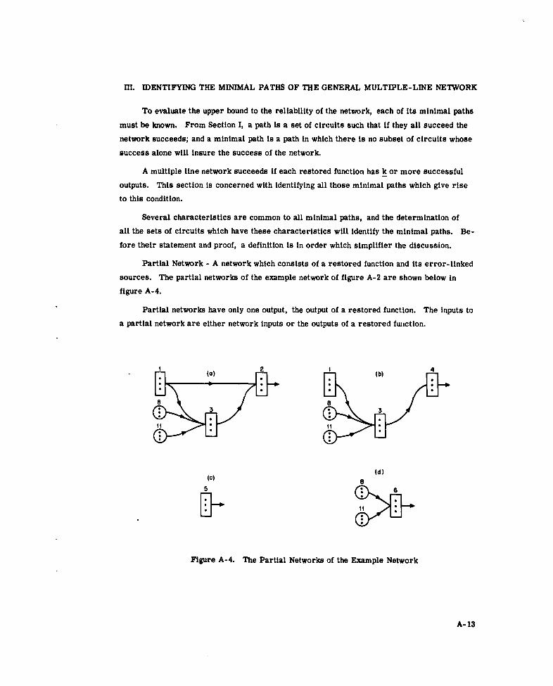
III. IDENTIFYING THE MINIMAL PATHS OF THE GENERAL MULTIPLE-LINE NETWORK
To evaluate the upper bound to the reliability of the network, each of its minimal paths
must be known. From Section I, a path is a set of circuits such that if they all succeed the
network succeeds; and a minimal path is a path in which there is no subset of circuits whose
success alone will insure the success of the network.
A multiple line network succeeds if each restored function has k or more successful
outputs. This section is concerned with identifying all those minimal paths which give rise
to this condition.
Several characteristics are common to all minimal paths, and the determination of
all the sets of circuits which have these characteristics will identify the minimal paths. Be-
fore their statement and proof, a definition is in order which simplifier the discussion.
Partial Network - A network which consists of a restored function and its error-linked
sources. The partial networks of the example network of figure A-2 are shown below in
figure A-4.
Partial networks have only one output, the output of a restored function. The inputs to
a partial network are either network inputs or the outputs of a restored function.
(d)(C) 8
Figure A-4. The Partial Networks of the Example Network
A- 13

The minimal paths of the partial networks are easily found and it will be shown later
that the minimal paths of the network may be found from the minimal paths of its partial
networks.
With the help of the partial network concept, the characteristics which identify minimal
paths are listed below.
1. Each minimal path will include circuits in every function and restorer in the
network.
2. The success of only the circuits in a particular minimal path will cause
exactly k particular output lines of each restored function to be successful;
the remaining m-k lines will be failed. The path is identified by the positions
of the k successful output lines at each restored function.
3. A minimal path of a partial network consists of k circuits from each function
or restorer in the partial network. All the circuits will be in the same
positions as the k successful output lines of the partial network.
4. With one minimal path chosen for each partial network, one minimal path
of the network will consist of all the circuits included in the chosen minimal
paths of the partial networks.
Proof of the first characteristic:
As the success of every circuit is necessary for the success of a nonredundant
network, the success of every function is necessary for the success of the redundant network.
Then circuits from every frunction must be included in each minimal path. A restorer
operates on the output lines of a restored function, hence the connections between a restored
function output and other functions in the network must pass through the restorer. Then the
success of the restorers are necessary to the success of the network and circuits from
each restorer must be included in each minimal path.
Proof of the second characteristic:
For purposes of this proof assume that only the circuits in a particular minimal
path are successful and that all other circuits are failed. Now assume that at the output of
one restored function there are less than k successful lines. These output lines are fed
into a restorer whose circuits can make the correct decision if k or more inputs are
successful, but since there are less than k successful inputs to the restoring circuits, they
will make the wrong decision, and all the outputs of the restorer will be failed. No restora-
tion can correct a set of completely failed lines so the network is failed. But it was assumed
A-14

initially that the circuits in a minimal path were successful and the network was successful.
Since the network cannot be both failed and successful, the assumptions are contradictory.
There must be at least k successful output lines at each restored function if the circuits in
a minimal path are successful.
Now assume there are more than k successful outputs of a restored function. Each
output line emanates from a different circuit. Then the set of successful circuits required
to assure the success of an output line in a particular position is different from the set re-
quired for the success of an output line in a different position. If the restored function has
more than k successful output lines and only k are required, some of these lines may fail
without causing failure of the network. This means that some of the circuitj necessary for
the success of these lines may fail without distrubing the operation. But it was assumed
that only the members of a minimal path were successful, an. by definition if members of
the minimal path fail, the network will fail. Then if only the minimal path is successful
there cannot be more than k successful output lines at each restored function.
Since there cannot be more or less, there must be exactly k successful output
lines at every restored function. The other m-k lines must be failed.
Now each minimal path is a particular set of circuits assuring successful operation
of the network. If at each restored function a particular set of k successful output positions
is chosen the circuits required to assure the success of these outputs are determined. These
circuits are a minimal path of the network. If a different set of successful outputs is chosen,
a different set of successful circuits is required and a different minimal path is identified.
Thus, the minimal path is identified by the positions of the k successful output lines at each
restored function.
Proof of the third characteristic:
Consider a partial network separately from the network as in figure A-4. Assume
that all the inputs to the partial network are correct. For a particular k output lines of the
partial network's restored function to be successful, all the circuits in the error-linked
sources of the restored function with the same positions as the successful output lines must
also be successful. This is because all the circuits in a particular position in the error-
linked sources of a function will affect its output line in that position. The failure of any one
of these circuits will cause the failure of that output line. Then in each partial network, k
circuits in each function must be successful for k output lines to be successful, and they
must be in the same positions as the successful output lines. This is a minimal path of the
partial network.
A- 15

Proof of the fourth characteristic:
Still keeping the partial networks separate, choose a set of k successful output
positions for each partial network output. From the foregoing discussion this determines a
minimal path for each partial network. These circuits can be listed and identified by their
number and position.
Now consider the network in its entirety, and assume the same sets of successful
output positions at each restored function as assumed in the last paragraph for the partial
networks considered separately. Since at each restored function there are exactly k
successful outputs, this network is now operating with only the circuits in a minimal path
successful. For a particular restored function in the network for a particular set of output
lines to be successful, the only requirements are; 1. that the network is operating success-
fully and 2. all the circuits that are in error-linked sources of the restored function and
are in the same positions as the successful output lines must be successful. The first
condition is fulfilled by our assumptions, and the circuits required by the second condition
are the same circuits that were in the minimal path of the partial network of the restored
function.
Then the list of circuits mentioned prevlously as the minimal paths of the partial
networks are sufficient to assure the success of k output lines at each restored function of
the network in its entirety. This by definition is a minimal path of the network.
To illustrate these concepts consider the partial networks of figure A-4. Each
partial network has (m) different minimal paths. With m=3 and k=-2, each will have three
different minimal paths. Identifying them by the positions of their successful output lines,
the minimal paths of each partial network are (ab), (ac), and (bc).
The example has four partial networks, and every different set of minimal paths for
the partial networks results in a different minimal path for the complete network. Then the
network has (3)4 = 81 minimal paths. Some of these paths are listed in table A-5 identified
by the numbers of the circuits in the restored functions whose outputs are successful.
It remains to determine from table A-5, the actual circuits that are members of a
particular minimal path. The circuits in a particular minimal path are all the circuits
in each of the minimal paths of its partial networks.
A-16

Table A-5. A Partial List of the Minimal Paths of the Network in Figure A-2
Min. Path Successful outputs in restored functions
2 4 5 6
1 (ab) (ab) (ab) (ab)
2 (ab) (ab) (ab) (ac)
3 (ab) (ab) (ab) (bc)
4 (ab) (ab) (ac) (ab)
5 (ab) (ab) (ac) (ac)
6 (ab) (ab) (ac) (bc)
7 (ab) (ab) (bc) (ab)
8 (ab) (ab) (bc) (ac)
9 (ab) (ab) (bc) (bc)
10 (ab) (ac) (ab) (ab)
11 (ab) (ac) (ab) (ac)
12 (ab) (ac) (ab) (bc)
etc. etc.
The circuits in a minimal path of a partial network are those circuits in the same
position as the successful output lines. For instance for the partial network of figure A-4(a),
the successful circuits required for the success of lines a and b are:
1 1 3a , 3 2a , 2 8 8 11 11a- b' a' b' a' b' a' b' a' Ib
The circuits in minimal path 1, of table A-5, are all those in positions a and b in the
network. The probability of success of a circuit in function i is p. Since there are two
circuits from each function or restorer in this minimal path, its probability of success is:
2 2 2 2 2 2 2 2
P1 P2 P3 P4 P5 P6 P8 P1 1
If a function or restorer is in more than one partial network, it will contribute three
circuits to the minimal path if the positions of the successful lines in the minimal paths
of the partial networks are different. For instance in minimal path 11, the minimal
paths of functions 2 and 5 are (ab) and functions 4 and 6 are (ac). The circuits in the
minimal paths of the partial networks are listed in table A-6.
A-17

Table A-6. The Members of a Minimal Path
Restored Function Minimal Path Circuits in minimal path
2 (ab) la, Ib, 2a ,
2b, 3a 3b,
8a 8, ,11a-, 11b
4 (ac) a 1c, 3a, 3 c, 4a 4c,
8a, 8c , 11a, 11c
5 (ab) 5a 5b
6 (ac) 6a 6c 8a, 8c , 11a, 11c
The circuits in this minimal path are then:a' 1b c, 2a , 2b
3a, 3b 3 c,
4a, 4c,
5a, 5b, 6a 6c 8a, 8b, 8 c)
11a 11b y 11c
The probability of success of this minimal path is:
3 2 3 2 2 2 3 3Pl P2 P3 P4 P5 P6 P8 P11
Functions 1 and 3, and restorers 8 and 11 have circuits common to two partial networks
with successful outputs in different positions. They contribute three circuits each to this
minimal path.
This section has shown that if one knows the error-linked sources of each restored
function in the network, the partial networks can be determined. The minimal paths of the
network can be found from the minimal paths of its partial networks.
A-18

IV. MATRIX TECHNIQUES
For the remainder of this report will generate a systematic technique which determines
the minimal paths and cuts of a redundant network. From this information, upper and lower
bounds on reliability may be found.
This section introduces a method, using Boolean matrices, which is simple, accurate,
and can be implemented on a digital computer. In this method one starts with a matrix
which describes all the primary error-linked sources of the functions in the net;,-ork. By
iterative operations on this matrix a composite matrix is formed which gives all the sources
of every function in the network. This section describes how this composite matrix is
determined for redundant networks.
Later sections will show how the composite matrix will be used to identify the minimal
cuts and paths of a network.
A. DEFINITIONS OF TERMS6
The discussion to follow uses Boolean matrices to describe topological properties of
digital networks. In the interest of clarity, this section is devoted to the explanation of all
the terms used and a description of matrix operations used in the analysis.
1. Boolean Matrix - A Boolean matrix is a rectangular array of I's and O's. A
general matrix is shown in figure A-5. The term aij is an element of the matrix at the in-
tersection of the ith row and 1 th column. An element may be either 0 or 1. The matrix is
represented symbolically by the element symbol within parentheses, (ai).
a 11 a12 . . a ln
a21 a22 . . a2 n
(aij)
anl an 2 . . ann
Figure A-5. General Matrix
A- 19

Multiplication of Matrices - The multiplication of two Boolean matrices,
(aij) and(bij) is indicated by the symbol ®& :
(alj) (8) (bij) = (cij)
The elements of(cij)are found from (aii) and (b.j) by the equation:
c =U a bij K ik k
The product and addition operations in the above expression are logical operations.
For the multiplication operation, alk . bkj = 1 only if both factors are 1. The symbol U
represents Boolean summation over all k. The addition operation, aik ' bkj + a * b =
lifeitheraik bkj orai " be j are 1.
2. Primary matrix - The primary matrix of a redundant network indicates the
primary error-linked sources of every function in the network and also the functions and
restorers which are present in the network. It is symbolized (Iij). The matrix has 2s rows
and 2s columns where s is the number of functions in the network. The first s rows and
columns describe the functions and the last s rows and columns describe restorers. A
restorer on the outputs of the kth function is described in the (s+k) th row and column. If
I is unity in the primary matrix, an output of function j provides an input to function i. In
other words, functionl is a primary error-linked source of function I.
The primary matrix indicates the functions or restorers that are present in the
network by entries along the principal diagonal where I = j. If I = 1 the function or restorer
i is present in the network. Of course, all the functions are always present in the network;
hence Ili = 1 for i 4 s. One of the design parameters in the redundant network is the place-
ment of restorers, so I (s+i) (s+-) = 0 if there is no restorer after function t.
To illustrate this discussion and to point out several characteristics of primary
matrices two redundant networks are shown in figure A-6 with their primary matrices.
The primary matrix is constructed from the flow graph by inspection with the
primary error-linked sources of each function listed in its rows. In example (a), l's
appear along the principal diagonal, or I = 1, for I, 6. This indicates that the six functions
are present in the network. For the rest of the elements along the principal diagonal,
i > 6, Ii = 0, indicating that there is no restorer after any of the functions. The 1 elements,
off the principal diagonal, indicate primary sources. For instance, the l's in elements
131 , 132 and 135 show that functions 1, 2 and 5 are primary sources of function 3. Elements
A-20
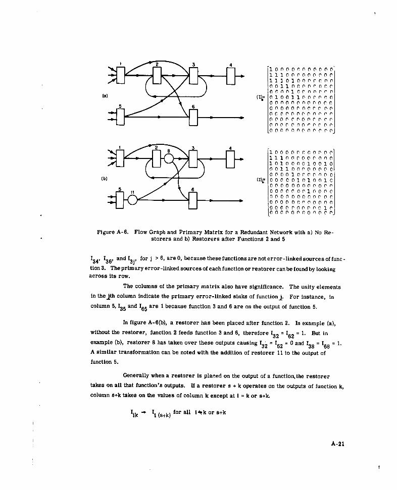
1 100 000 00 01 10100 n 0C
0 o nOnn
(0) 01 00 1 10 0 Crn (
" 0 0 0 0 0 0 0 C C r r
= 00CCOOO00Co CC*0 0 C C 0 C C C C C, C Cj
1OO O OOC 00
0 0 0 0 0 1 0 1 0 0 1 0O ()0 01O0 ) ( 0 0(b) (Il;= 0 0 0 0 0 1 0 1 0 0 1 0
0000000000 nC0000 00 00000000000O0000010O0000000000
Figure A-6. Flow Graph and Primary Matrix for a Redundant Network with a) No Re-storers and b) Restorers after Functions 2 and 5
134, I36 and I3j, for j > 6, are 0, because these functions are not error-linked sources of func-tion 3. The primary error-linked sources of each function or restorer can be found by lookingacross its row.
The columns of the primary matrix also have significance. The unity elementsin thelth column indicate the primary error-linked sinks of functionj. For instance, in
column 5, I35 and 165 are 1 because function 3 and 6 are on the output of function 5.
In figure A-6(b), a restorer has been placed after function 2. In example (a),
without the restorer, function 2 feeds function 3 and 6, therefore 132 = 162 = 1. But in
example (b), restorer 8 has taken over these outputs causing I32 = I62 = 0 and I = 168 = 1.A similar transformation can be noted with the addition of restorer 11 to the output of
function 5.
Generally when a restorer is plared on the output of a function, the restorer
takes on all that function's outputs. If a restorer s + k operates on the outputs of function k,
column s+k takes on the values of column k except at i = k or s+k.
I " Ii (s+k) for all itk or s+k
A-21

With a restorer on its output, function k no longer can be an input source for
any function, so all the elements in column k are 0 except Ikk.
I1k = 0 for all I it k
The presence qf a restorer must be noted in the primary matrix along the
principal diagonal. For instance, for example (b), elements I88 and I(,,) (,,) are 1. These
restorers do not remove function 2 and 5 so I22 and I55 remain 1.
Generally, with function k and restorer s+k both in the network, along the
principal diagonal:
Ikk = I (s+k) (s+k) - 1
The primary error-linked sources of function k do not change because of the
addition of restorer s+k, so the kth row does not change.
From the definition of primary error-linked sources,the restorer has none.
In general, for all rows describing the inputs to restorers, all elements are 0 except along
the principal diagonal.
I(s+k)i =0forall iA- s+k
The symbols representing functions and restorers in figure A-6 have been
purposely left empty to indicate that the primary matrix is independent of the order of re-
duidancy of the function and restorers.
The characteristics listed above hold for all primary matrices.
3. Secondary Matrix - The secondary matrix has the same form as the primary
matrix and is symbolized (I1ij). In addition to indicating what functions or restorers are
present along the principal diagonal and the primary error-linked sources, the secondary
matrix also indicates the secondary error-linked sources. An element IIj with a value 1
indicates one of three things;
a. if I = j, function i is in the network,
b. j is a primary error-linked source ofi
c. j is a secondary error-linked source of i.
It is impossible to tell from the secondary matrix whether an element indicates a primary or
secondary connection. The secondary matrices for the examples shown in figure A-6 are
shown in figure A-7.
A-22

100000000000" "10000000000 0
111010000000 111000010010
1110100000001 101000010010
1111100000001 101100010010
000010000000 000010000000
(I) = 11101 1000000 (H)b 000001010010
000000000000 000000000000
000000000000 000000010000
000000000000 000000000000
000000000000 000000000000
000000000000 000000000010
000000000000 000000000000
Figure A-7. The Secondary Matrices of the Example Networks of Figure A-6
4. nth order Matrix - This is the general case of which the primary and secondary
matrices are particular cases. The nth order matrix is symbolized (Nil), and it indicates
all nth and lower order error-linked sources.
Since the nth order matrix includes all the (n-1) and lower order error-linked
sources, each element of the nth order matrix must be equal to or greater than the correspond-
ing element of the (n-1) th order matrix.
Hence
N ij N-j N-2j... ; U(A-5)
Elements that are 1 in (N1l) but 0 in (N-lij) are nth order interconnections.
5. Composite Matrix - This matrix shows all the error-linked sources of every
function in the network. It is defined as the nth order matrix for which:
(N)ij = (N+k)j k= 1, 2... foralli, j
or every element in (N1i) is equal to the corresponding element in higher order matrices.
Once a matrix is found such that a higher order matrix has the same elements,
this is the composite matrix.
A-23
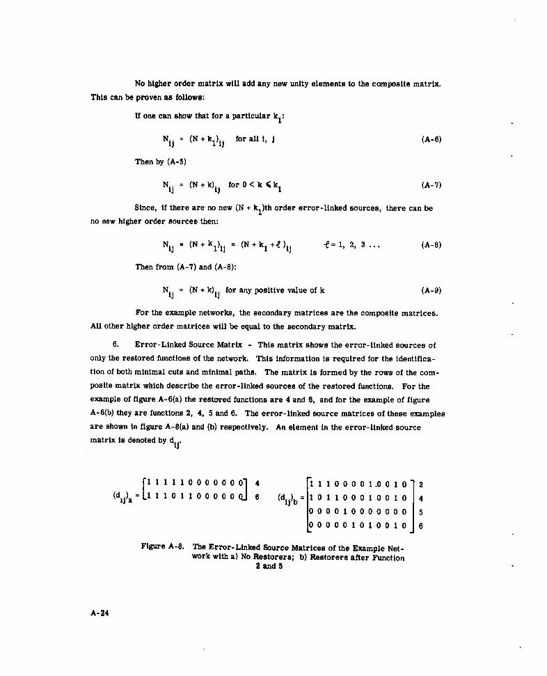
No higher order matrix will add any new unity elements to the composite matrix.
This can be proven as follows:
If one can show that for a particular kl:
Nij = (N + kl)ij for all i, j (A-6)
Then by (A-5)
Nij = (N+k)ij for 0< k 4k 1 (A-7)
Since, if there are no new (N + k1)th order error-linked sources, there can be
no new higher order sources then:
Nij = (N+kl)ij = (N+k 1 + )1 i "- = 1, 2, 3.... (A-8)
Then from (A-7) and (A-8):
Nij = (N + k)ij for any positive value of k (A-9)
For the example networks, the secondary matrices are the composite matrices.
All other higher order matrices will be equal to the secondary matrix.
6. Error-Linked Source Matrix - This matrix shows the error-linked sources of
only the restored functions of the network. This information is required for the identifica-
tion of both minimal cuts and minimal paths. The matrix is formed by the rows of the com-
posite matrix which describe the error-linked sources of the restored functions. For the
example of figure A-6(a) the restored functions are 4 and 6, and for the example of figureA-6(b) they are functions 2, 4, 5 and 6. The error-linked source matrices of these examples
are shown in figure A-8(a) and (b) respectively. An element in the error-linked source
matrix is denoted by dii.
[ 11 10000000 4 1 1 00001- 0 012
(d j) a = 1 1 0 1 1 0 0 0 0 0 6 (dij)b = 1 0 1 1 0 0 0 1 0 0 1 0 40000100000001 5
00001010010 6
Figure A-8. The Error-Linked Source Matrices of the Example Net-work with a) No Restorers; b) Restorers after Function
2 and 5
A-24

B. DETERMINATION OF THE COMPOSITE MATRIX
Given the primary matrix of a network, the secondary, tertiary or any order matrix
may be determined. Multiplying the primary matrix by itself gives the secondary matrix.
Thus:
(I (Il) =
To illustrate why this occurs,an element 1ij results from the boolean operation:
Ij = U I .
ij K~ ik ' kj
When for a particular k not equal to i or.I, Ilk ' = 1, then function k must be a
primary error-linked source of function I, and functionj must be a primary error-linked
source of function k. Then function! will be a secondary error-linked source of function I.
Ifj is a primary error-linked source of i, Ij = 1. Functionj must be in the network,
then 1j = 1. One of the terms in the summation determining IIj will be:
Ij • Ijii 1 1 ij
So the secondary matrix also indicates primary error-linked sources.
An element on the principal diagonal of the secondary matrix IIi1 will be unity if
function i is included in the network.
Hii * I ii = 1
It should be readily apparent, by the same reasoning, that the tertiary matrix results
from multiplication of the primary and secondary matrices.
( ij) = (1i) ® (Iij)
In general, the nth order matrix is the product of the (n- 1)th order matrix and the
primary matrix.
(N Ij) (N-11j)(&(Iij)
The composite matrix is found when this operation is performed and
(Ni) = (N-Ij)
A-25

So successive multiplications of higher and higher order matrices by the primary
matrix will eventually result in the composite matrix.
The composite matrix is found with fewer multiplication operations if it is recognized
by the associativity property of matrix multiplication,
P(iVj) =f (I ij) (llj) (Iij) (Ilj ) = (11 ij) (r1ij)
The quanternary matrix is the square of the secondary matrix. By first squaring the
primary matrix to obtain the secondary matrix, then squaring the secondary matrix to obtain
the quaternary matrix, then successively squaring the higher order matrices until there is
no further change in the matrix, the composite matrix will finally be reached.
A-26

V. DETERMINING THE MINIMAL CUTS OF A NETWORKFROM ITS ERROR-LINKED SOURCE MATRIX
In the last section the composite matrix was obtained which indicated the error-linked
sources of each function in the network. Section IV. A described the derivation of the error-
linked source matrix from the composite matrix. The error-linked source matrix and the
characteristics of minimal cuts described in section II are sufficient to enumerate all the
minimal cuts of a general multiple line network. The first part of this section will show
how the minimal cuts are found for the network of figure A-2, when the network has redundancy
of order three. The second part will generalize this discussion so that functions may have
higher orders of redundancy, and the restriction is removed that all functions must necessa-
rily be the same order of redundancy.
A. ORDER THREE REDUNDANT NETWORK
The minimal cuts of the order three network of figure A-2 will be determined from the
error-linked sources of the restored functions of the network. This matrix is shown in
figure A-9.
1 2 3 4 5 6 7 8 9 10 11 12
2 1 1 10000100 1 0
4 1 0 1 1 0 0 0 1 0 0 1 0 (dij)
5 0000100000 0 0
6 0000010 100 1 0
Figure A-9. Error-Linked Source Matrix for Network of Figure A-2
For an order three network, the minimal cut will consist of 2 circuits, each in a
different position and each either in the restored function or in its error-linked sources.
There are two kinds of minimal cuts in an order 3 network. The first kind includes
those cuts in which both circuits are in the same function or restorer. Every function or
restorer in the network will contribute this type of cut. The probability of failure of a cut
of this nature in function x is:
(1-Px) 2 (A-10)
A-27

There are three ways to choose the circuits which are failed in a particular function
or restorer. Then each will contribute three minimal cuts. The probability that failure
does not occur due to failure of minimal cuts of the first kind is:
r1- d(A-11)allL al
The symbol U is used to represent Boolean summation. The factor U d is I iffor a given j.(column) there is some row in which d = 1. If U di. = 1, function I is
ij all Iipresent in the circuit. For example if j = 3:
d13 = d23 + d43 + d5 3 + d 63 = I + I + 0 + 0 = 1
Indicating that function 3 is in the network and contributes minimal cuts of the first
kind. For j = 9
dig d29 + d49 + d59 + d69 = 0 + 0 + 0 + 0 = 0
Restorer 9 is not in the circuit and the factor:
[1 (1-P 9 )2] =1_ all, i9 1-
There is no chance of failure of minimal cuts in restorer 9, because it is not in the
network. For the network whose error-linked source matrix is that of figure A-9 the proba-
bility that failure does not occur due to failures of the first kind is:
The second kind of minimal cut includes two circuits, one in each of two functions or
restorers. As described in section II, two circuits are in the same minimal cut only ifthey are both error-linked sources of the same function. The error-linked sources of
function 2 are functions 1, 2 and 3 and restorers 8 and 11. A minimal cut of the second
kind will include one circuit from each of two of these functions; circuits in function 3 and
restorer 8 for example. The probability of failure of a minimal cut of type 2, one in func-
tion x and one in function y is:
(i-px) (1-py (A-13)
A-28

Minimal cuts of the second kind are present in functions x and y only if the Boolean
equation:U dd =1 (Ai
d~ ix diy Ixae dy (A- 14)
all I
is satisfied. Equation 14 says that both x and y are error-linked sources of the same re-
stored function.
Then the probability that a cut of the second kind does not fail in functions x and y is:
1- ( U d d ) (i-px) (l-p) (A-15)x.~qy ix iy x y
all I
Circuits in the same position cannot be in the same minimal cut. There are three
positions from which the first member of the minimal cut may be chosen from function X
but once this choice is made, there are only two positions in function y from which the
second member of the cut may be chosen. Then there are 6 minimal cuts which include one
circuit in function x and one circuit in function y.
With this information, the probability that a minimal cut of the second kind does not
fail in a network can be written:
7 1 -(U dixdiy (1-Px) (1-py (A-16)all x y xy
all i
Now with the results of (A-11) and (A-16) the total minimal cut reliability expression
for an order 3 multiple line network is written:
d T dx) (1_Px)2 U d]6 (-x)(-
RLB al-l ( a -( all d )apllp ] all-( U didyyL ix [J) U, alli y (A-17)
The values of dIx are obtainable from the error-lined source matrix, and the reliabili-
ties of the individual circuits in the network are assumed given; then for an order three
multiple line network the minimal cut lower bound on network reliability can be calculated
from the formula given above.
B. GENERAL MULTIPLE-LINE NETWORKS
The information contained in the error-lined source matrix and the reliabilities of
circuits in the network are sufficient to determine the minimal cut reliability for any multiple
A-29

line network which fulfills the conditions of Section HI of the text. For orders of redundancy
greater than three, however, the determination of the minimal cuts will be more difficult.
Say a restored function has order m redundancy and at least k of its output lines must be
functioning or system failure results. Then there will be m-k+1 circuits in each minimal
cut associated with the output lines of this restored function. These circuits may all be in
the same function, there may be une in each of m-k+1 functions, or there will be some dis-
tribution of the circuits among some intermediate number of functions.
The minimal cuts of the network will be divided into a number of kinds as to the
number of functions represented in a minimal cut. The first kind has all its circuits in one
function, x. The probability that m-k+i circuits of type x fail is:
(i-px) m-k+l (A- 18)
There are (Mk+1 ) distinct sets of circuits in x that will form a minimal cut of the
first kind. Then the probability that none of the minimal cuts of the first type fail is:
7x[1- U , x)(-p ,m-k+1 , m - k + 1 ) (A- 19)all x all
The minimal cuts of the second type have all their members in two functions. The
two functions are x and y. Assume that " of the members are in function x. Then
m-k+l- Vx = . y, the number of members in function y. The probability of failure of
particular minimal cut of this type will be:
(1-px) (i-py) _ y (A-20)
Whether circuits in functions x and y can be in the same minimal cuts is determined
by the Boolean operation:
U dlxdiy (A-21)
all I
There are (mx) ways the . circuits can be chosen from function x and (m vyx)
ways the 4 circuits in function y can be chosen from the available m- " x positions. Then
the probability that the minimal cuts of the type described do not fail is:
I-(a dxd (1-P) ox (1-py (nx I x (A-22)
A-30

Theexonnt(mn) (m-The exponent 4 x) can be written:
y
(mIx) (m - IX) = m i (A-23)
x yx -Oy 7-1 7y 1 (k- 1)1
Where Px + Oy = m-k+l
and l , .e i
x y
To obtain all the minimal cuts of the second kind all the possible values of Ix and
4 must be considered, and all the possible combinations of two functions in the network
must be included in the equations. The probability that a minimal cut of the second kind in
the network does not fail is:
allx,y all { 4 m I
X'y Lx +Oy = mk+- ix 1
In general, the minimal cuts of an order m network will be of the first, second up to
the m-k+1 th kind. The general expression for the reliability of the minimal cuts of the cc
kind can be derived in a manner similar to the expression above. In general the probability
that minimal cuts that are distributed among Cc functions do not fail is R( C), given by
all x, y, z' Ua x, y, P. • Il- (1 - ddixdy di e)
my
x ey .z ,x! _y!_z!•1PX 1Py) (-z ... ' '-M (A-25)
Where x4 y Iz... * tc
"x 4+ + V + ....- +' -= m-k+1
--x,i
I A-31

Equation (A-25) is the general equation, all other equations in this section can be
derived from it. It gives the probability that a minimal cut of the a kind does not occur,
where a can be 1, 2 ... m-k+l. The lower bound to network reliability is probability
that none of the minimal cuts fail or:
RLB = R (1)R (2)R (3) ... R (m-k+l) (A-26)
C. DIFFERENT ORDERS OF REDUNDANCY
Since the order of redundancy of an input source is the same as the order of
redundancy of its restored function, the orders of the restored functions in the network de-
termine the order of every function in it. Each line in the error-linked source matrix can
be assigned an order of redundancy which will apply to each function which has a unity
element in the line. Since a function can be only one order of redundancy, lines with common
unity elements must be of the same order. For the example in figure A-9, lines 2, 4, and
6 which include functions 1, 2, 3, 4, 6, 8, and 11 will all be the same order of redundancy,
and line 5, which includes function 5, may be another.
To analyze the minimal cut reliability of a network with more than one order of
redundancy, the error-linked source matrix can be broken into a number of smaller matrices
such that each matrix includes only functions with the same order of redundanc-. Then the
network is considered as a number of smaller networks each with only one order of re-
dundancy and analyzed in the manner already described. The overall network reliability is
the product of the reliabilities of the smaller networks.
A-32

VI. DETERMINATION OF THE MINIMAL PATHS OF A NETWORK FROMITS ERROR-LINKED SOURCE MATRIX
Section I stated the characteristic that a minimal path of a network will consist of
the circuits in the minimal paths of its partial networks. The error-linked source matrix
describes exactly the partial networks. A particular row in the matrix lists all the error-
linked sources of one of the restored functions and these are the functions that will be
connected to the restored function to form the partial network. There is one row for each
restored function in the network, so all the partial networks are described by the error-
linked source matrix. This fact is illustrated by noting the partial networks of the example
network in figure A-4 and its error-linked source matrix in figure A-9.
The determination of the minimal paths of the order-three example network from its
partial networks has already been accomplished in Section ITT. The general problem will
be solved in a similar manner.
The positions of k successful output lines will be assigned to each partial network,
and the circuits in the minimal paths of the partial networks identified by the third characteris-
tic of Section I. One minimal path of the network will be the circuits in these r,'inimal
paths of the partial networks.
Every different arrangement of successful output lines oi the output of the partial
networks will result in a different minimal path of the network, so they all must be con-
sidered. In general, the ith partial network will have (mi ) minimal paths. Then the totalk Inumber of minimal paths for a network with/, restored functions will be:
The probability of success of a minimal path must include factors representing the
reliability of the circuits in each function. The only difference between the reliabilities of
the different paths will be the exponents of the various circuit reliabilities. In general,
the reliability of a minimal path is:
al ( Pt '
Where i Is the reliability of a circuit in function i. The exponent v is the number
of circuits in function i that are members of the minimal path. For a particular function,v may vary between k and m. If the function is in only one partial network will always
g A-33

equal k, since only k positions are required to be successful for the success of a partial
network. If the function is in 4_ partial networks I may vary between k and I k or m,
whichever is less. To illustrate this consider one function, of order five redundancy with
k=3, which is common to two partial networks. Table A-7 provides a list of v for this
function for three choices of successful output positions for the partial networks. The five
positions are a, b, c, d, und e.
Table A-7. List of Successful Outputs of Partial Networks in a Minimal Path
No. Successful Output Successful Output Circuits in the viPositions of Partial Positions of Partial Function in theNetwork 1 Network 2 Min. Path
1. a, b, c a, b, c a, b, c 3
2. a, b, c a, b, d a, b, c, d 4
3. a, b, c a, d, e a, b, c, d, e 5
The problem is to determine Yi for each function and for each minimal path. At
present this is a difficult problem to solve without excessive effort. The solution has
already been outlined. Every possible minimal path must be tried, and the necessary cir-
cuits must be determined for each minimal path. This is a very large effort for all but the
simplest of networks since a multiple line network will have a very large number of
minimal paths.
A-34

VUI. DETERMING RELIABrLITY WHERE ONE FUNCTION IS AN ERROR-LINKE.D..SOURCE OF TWO OTHERS OF DIFFERENT ORDERS OF REDUNDANCY
In some instances, due to the relative values of reliability of different circuits, it may
become desirable to assign different orders of redundancy to functions in the multiple line
network. If the redundancy is applied such that there is no function in the network that is an
error-linked source of functions of different orders of redundancy, the analysis will remain
the same as in Section V C. of this Appendix. However, if the case should arise where one
function is an error-linked source of two functions of different orders of redundancy a cer-
tain amount of difficulty will be introduced into the minimal cut reliability analysis, and a
more complex expression for the reliability of the network will result.
Consider a network in which there is a juncture where a function feeds two other
functions of different orders of redundancy. Function Z in figure A-10 is such a Juncture
Function.
For this analysis, the assumption is made that the juncture function is of the same
order of redundancy as the higher of the two which it feeds. It has, as its error-linked sources,
functions of order of redundancy equal to itself
A. FIRST KIND OF CUTS
The number of first kind of cuts in function Z of figure A-10,which is an error-linked
source of functionsa, and c2, is described by the following expression:
0(.e 4M k +) _1 m2(A-27)
where: m 2 is the order of redundancy of the lower order function
I 1 is the order of the function in question, or of the higher order function
k2 = number of correct outputs necessary for a function of order m 2 to produce a
correct output
k 1 = number of correct outputs necessary for a function of order m 1 to produce a
correct output
= the number of failures occurring in those elements of function Z which feed
both function c 1 and Munction 2"
A-35

This expression indicates the number of minimal cuts which can occur which will
cause the outputs of function c or a2 to be false. The first term indicates all the possible
combinations of circuit failures in function Z which include less than (m2 -k2 +l) failures in
the circuits which feed both function 1 and function c12. More than (m 2 -k2 +1) failures in
this group would cause function o2 to have an incorrect output; hence, any combinations
including these failures would not then be minimal cuts.
There are also minimal cuts which will cause the output of function CL2 to be false.
These are failures of (m2 -k 2+1) circuits in the m2 circuits which feed function cx2 , and this
number is obtained by second term of the above expression.
Since functions X and Y feed function Z, and are of the same order of redundancy,
failures in any circuit in X or Y will cause an incorrect output of the corresponding circuit
in function Z. Hence, the equation describing the minimal cuts of the first kind for functions
X and Y is the same as for Z. Therefore, this expression yields the number of first kinds
of cuts for any function which is an input source to two functions of different orders of
redundancy.
If it is now assumed that functions a1 and /31 feed only functions of order m1 or
higher redundancy the number of minimal cuts of the first kind in each of these functions is
merely the number of combinations of (m1-k1 +1) elements out of a possible m 1 elements
(i.e.)
The same analysis holds for functions c2 and /2 yielding the expression for the number of
first kind of minimal cuts in each function:
(m2 k 2 +) (A-29)
The reliability due to the first kind of minimal cuts for this configuration is:
r / ( m-k2 1)km1 ++1J
-- g Q (a l i d i g )- k 1R(I u d g .1-
Sdig ) (1P (A-so
b A- 37

ksRK~l - ~ dikMi- (;k +)
all (ml-kl+l)
7- U dit t
where: g, k, t are dummy variables referring to the functions which are members of the
sets, Q, R, S, respectively.
This equation is of the same general form as those derived in Section V B. of this
report.
The following definitions are of importance to the discussion of second and higher kinds of
cuts and will be used in the subsequent development:
Q = set which includes all functions which are error-linked sources of botha 1and or IZ, Y, X, ... I
R = set which includes all functions of order m1 which are error-linked sinks
of the juncture function [ /11 t ... I
S = set which includes all functions of order m 2 which Ire error-linked sinks
of the juncture function [ M 2' /32' " "I
Sdi ) refers to a Boolean summation over all i; where i takes on allall i I- _
number designations of restored functions and outputs.
p Pk and Pt are the reliabilities of the circuits in the g, k and t functions
respectively.
B. SECOND AND HIGHER KINDS OF CUTS
There exist, between the functions of order of redundancy m, whether before or
after the juncture, minimal cuts of the second and higher kinds. Because the functions in
the set Q are error-linked sources to two functions of different order redundancy, they must
be subdivided into two parts each--- those circuits which feed only the circuits of functions
in set R, the higher order functions after the juncture; and those which feed circuits in all
the functions after the juncture (i. e. circuits in functions of sets R and S)
A-38

Referring to figure A-10,it can be seen that circuits in function X which eventually
feed both functions a 1 and 2 need fewer failures among them to cause a false output in
function a2 than are required to cause the output of function C1 to fail. Hence, those cir-
cuits in function X feeding all the functions after the junctures are labeled X 2 and those
feeding only the higher order functions are labled X The number of failures which occur
in these groups, X 1 and X2, will be referred to as "0x1' and "'x2 respectively. The same
notation will hold for all other functions which are of order n 1 and are error-linked sources
to the juncture function. In order to calculate the reliability of a system, it is necessary
to find the total number of minimal cuts of the second and higher kinds between 1) functions
in the sets Q, R, or Q and R, 2) functions in the sets Q2 ' S or Q2 and S. Q2 is the set
which includes all groups of circuits (X2, Y2, Z 2 ... ). The number of minimal cuts are
subject to certain limitations. These will be discussed first.
The number of failures which can be allowed in the circuits which feed all the error-
linked sinks of the juncture function is limited. If this number (... + _e2 + _y2 z3) , exceeds
m 2-k2, the cut would not be minimal because more than enough failures will have occurred
to cause the output of function 2 to be false. Therefore, any combinations of more than
(m2-k 2) failures in X2, Y2 and Z2 with circuits in X1, Y1 and Z would no longer form
minimal cuts and should not be considered as such. Hence, 0 (... +..8 +'P +z) £
m2 -k 2.
A number of failures less than or equal to m2 -k 2 can combine with failures in the
circuits of the (X1, Y1 """) group to form minimal cuts which cause the outputs of the
higher order function, the set R,to be false. The possiblity is also present that the number
of failures necessary for the minimal cut could be confined to the (... X1, YI' Z1) group.
In any case the sum total of circuit failures must be equal to (m1 -k1 +1) I.e. (... '42 +
-" 2Y2 +4. + +.,OX +,Yl + eZ) = ml-kl+1. For this part of the analysis it is assumed
that the functions of order m 1 which are error-linked sinks of the juncture function will
be input sources only to functions of the same order.
1. Second and Higher Kindt of Cuts Between Functions of Set Q, R, or Q and R
It is desired to form aniexpression for the possible number of minimal cuts which can
exist between 2 or more functions of order m1 redundancy which may be either sources or
sinks of the juncture function. All the minimal cuts in the class will disable m1-k 1+1
output lines of one or more of the functions in set R.
A-39

For a second kind of cut only two functions will be taken at a time; for third
kind, three functions, fourth kind, four functions, etc. If a second kind of cut is being
examined, the circuit failures in two functions must total (m-k 1 +l).
a. Second Kind of Cuts for Furctions in Set Q
If these functions are chosen to be the juncture function and/or its error-
linked sourcesthe expression for the number of minimal cuts for given yl 1 Y, 1 '%4423 is:
Q ( e z 2) tz1,2 P (m lfm 2) (m 2- -&e) ( m~ 2 4 ,)
in which 'ez2 is the number of failures which are present in the Z2 group and ( ez2 ) the2
number of ways in which the -e failures can be chosen from the s 2 circuits in the Z group.Q2 2
Out of the remaining circuits in the function Z, another group can fail, "( 1 ) i." z
is the number of ways of choosing these failures. Once -4 circuits have failed in group Z
only (m2 - 1z2) circuits can fail in function Y2 which will affect an output which is not
already incorrect. There are m 42z2) ways of choosing these failures. There arey
gru ndthy ca fail y
failures which can occur in the Y) group and they can fail in 1 2 Zlways. This
expression can be expanded for three functions, four, etc.
b. Second Kind of Cuts for Functions in Set R
For the case where all the minimal cuts are to be considered in the R set
the expression becomes:
m 1
c. Second Kind of Cuts for Set Q and R
If one function represented in the minimal cut is the juncture function or oneof its error-linked sources, and the other is one of the higher order functions which are
error-linked sinks of the juncture function, the expression becomes
eR', ~) m (2 )( ml-2) (m,-ex-ox)
The third combination results because it now does not matter where in the function a
the failure occurs.
A-40

d. General Expression for Second and Higher Kind of Cuts in Set Q, R, or Qand R
This expression can be expanded and generalized to include all possible
combinations of functions, two, three, four or more at a time. For a second kind of cut all
combinations of 2 functions are taken and all values of the -e 's within the limitations, are
selected. For third kind of cuts, all combinations of 3 functions are taken and all values
of t 's, within the limitations, are selected, etc.
The final general expression for the number of minimal cuts of the second or
higher kind present between functions of order m1 redundancy either before or after the
juncture is as follows:
( Q, -R) () = ) ml-mn 2"2)n ml2nm2"z mm2- ) Omlzm 2l-1 1 - 1
(M. x '. + ' , 'x +1 '+ +
*(rni(... +.i+~ + <' P 1 +.. 2+ 2+'P.)..
X1+?1+?zI + 1 + x + +? + t ,+ I$,+... =M m k 1+1
2+ 2 'z2 1m2k2
S... e+ e -ez2 oi• " 'x+ex e+e ~+ ' 1+ 2' 1 2z ' ' ' " ** 1
expanded, the expression becomes
(#, P) = m2! (m -m,)! (m2-42)1 (m1-m2-- !
z2-! (m2 - e22) ! 21 ! (ml-m2 -z) ! 42! (m2- ez2 -'y 2)! eY l!(mI-m 2- 'e 1-42
(m2" 4z 2"'Y2 ! mlm 2- lezl - ' Y I [
Ix 2 I (m2"ez2- "Y2- x2)I 'Xl (mx-m2-1'zl- yj- x)
A-41
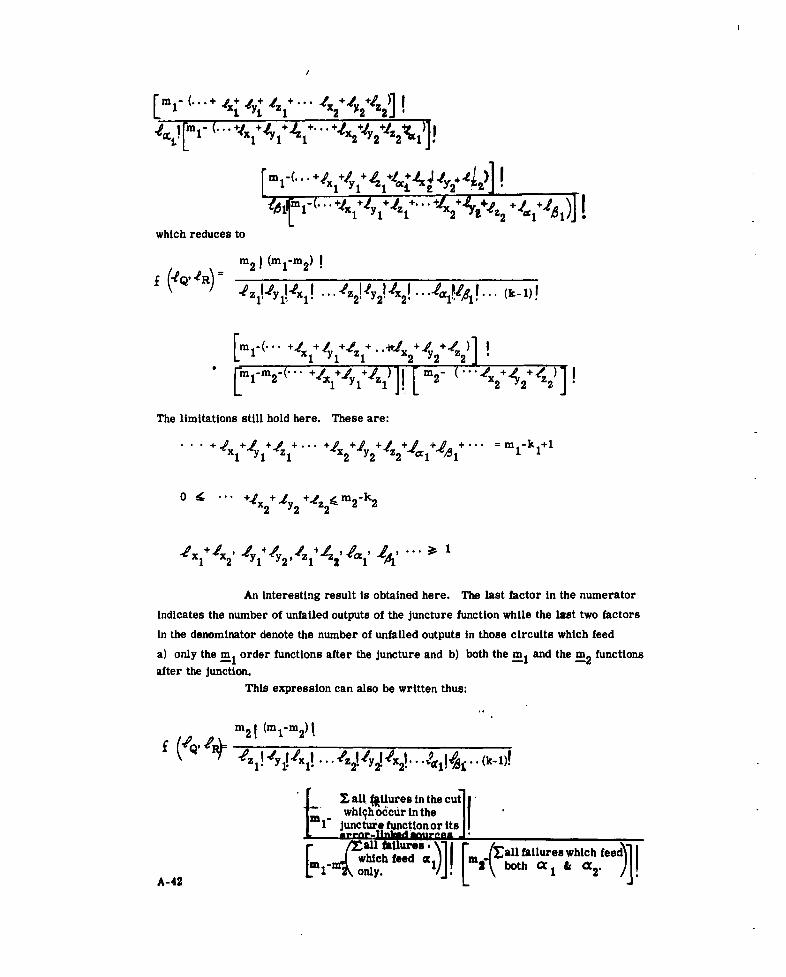
F~~~~ (...+42 ** +j /Xjx' 11 +,e +1 Z j -,
1 y 1 2x 2 211
which reduces to
m2 1m 1 m2 11/5. ... (k-i)l
+"# 4 4 I z2)~~1 I
X' 1' 1-.
[-(.In +/+1+1+O m11+)
The limitations still hold here. These are:
o -O -/Z +~ +0' ml-m
0 4 --- x2 + 1 2 +,z2 2k
Ox~x + l2~~ 4 # ... > 1
An Interesting result is obtained here. The last factor in the numerator
indicates the number of unfailed outputs of the juncture function while the last two factors
In the denominator denote the number of unfailed outputs in those circuits which feed
a) only the m1 order functions after the juncture and b) both the mand thems2 functionsafter the junction.
This expression can also be written thus:
L ~ -OZ 1 z1 !y _P!1 1 4zl 2
1 x I 1?!i; (k-i1)!
I. ! all. (ilures in the cutwhiqhodcur in theJ
ju ctre fqncin or its
[ rr allhc fed1falures which feed
A-2[n only. btCC1& X2 If

This expression yields the total number of minimal cuts of second or higher
kind between functions of order m I redundancy which are either error-linked sources to the
two output functions of the juncture function or error-linked sinks of the juncture function.
For the casc where the failed circuits are located before the juncture, in set Q, the ex-
pression reduces to:
'04 2!m,-m2)!S y 1 4 ! ... [ 4( [Yx 2 " " .m l -m 2 - (x l 1 4 l+ ' ) ]
My P' 2.1 2 2! **.. 1 1 Zi
I V+1e +10+
In the case where all the failures are located after the juncture, in set R, this expression
reduces to
mil
which is the same form as for minimal cuts between 2 or more circuits in a system of a
single order of redundancy.
2. Second and Higher Kinds of Cuts in Sets Q2P S or Q2 and S
Minimal cuts will also exist between functions in set S, (c a2, /6, ... ) and
circuits in the Set Q2 . Since the only circuits in functions (X, Y, Z, ... ) of set Q whose
failure can affect the output of the functions in set S ( a2' /32, . . .) are those which feed
all the functions after the juncture function, minimal cuts between these functions will in-
clude only circuits in the set Q2" Hence, as far as the functions in set S are concerned
they are being fed by functions of the order m 2 redundancy only, and the minimal cuts
present are the same as though this was a system of order m 2 redundancy. The number of
minimal cuts of the second and higher kinds between functions in the set Q2 and functions in
set S is found from the expression:
2 2! Y2! 4 2! 62!'" (k
A-43

If all the minimal cuts are considered to be after the juncture, in set S, the
expression becomes:
m 2! ..
£ (5) = 2
C. RELIABILITY DUE TO SECOND AND HIGIgEs KINDS OF CUTS
With these expressions it is now possible to write tht expression for the reliability
due to the second and higher kinds of minimal cuts of such a connection.
allx. y, z cc, , ,
R(2, 3, )= taken C at a time,
where C is thekind of cut. [ alli
I- (U d IXdty d iz " dicc' di'6 ...
+ "2 IY -YP 'z 2 -0a I (, "R>(1-P (1-Py) (1-P ) 2 1 " 'I '1
x +lx -4+ 44 Z+I-e- ,'"2' 1 2P 1, 2,':1 1r , 1
+1 x 2+Y2+ 42 5 'i2 -I 2
+,ex 1+Y 1+lZ1+... +Ix 2 +'eY2+z 2 +'1+ 1+ ... =M1-k1+1
R(2, 3,• .) allx, Y , z, €2, 2" ' 1.. d .. dR"2 3, 7' 2, A2 7r[-UlId ~. d 62d
lox Ie -& i zI ,(I- ) (IP ) 2 (-P" A 2 (" 2 ' ' PS I2
( -x y ) (1-y)PN . .
+x 2+ Y 2+1
2 +2 + / = i 2 - k 2 +1
A-44

-Ix2, 42, 0Z2, 42, 02,"
R(2, 3. .. )= R'(2, 3,...) (R"(2, 3,...)
D. TOTAL RELIABILITY
The total reliability of the system discussed here is the product of the reliabilities
due to the different kinds of cuts.
Rtotal= R(1) R(2)R(3)
A-45/46

VIII. DETERMINING RELIABILITY WHERE ONE FUNCTION IS AN ERROR-LINKEDSOURCE OF ANOTHER WHICH IS OF HIGHER ORDER REDUNDANCY
In the case where a function, in a network, may be less reliable than the rest of the
network, it may become necessary to assign this function a higher order of redundancy than
the other functions. If this function is not the first in the network it must, therefore, be
fed by a function of lower order redundancy than itself. This presents a problem in solving
for the network reliability.
There are two methods for connecting such a function and its source: (1) insert a
restorer on the output of the source , as in figure A-1, (2) connect the source directly to
the function of higher order redundancy as in figure All.
The first choice presents no problems if the restorer is assigned the same order of
redundancy as its primary sink, the higher order function. This results because, when the
restorer is inserted, the two functions are isolated from one another. The only minimal
cuts which exist are those between the restorer and the higher order function. Since these
are of the same order redundancy the reliability problem can be handled by methods
previously mentioned.
The second choice, that of not using a restorer, leads to more difficult relationships
between the two functions.
Because the function is of lower order than its sink, there are more circuits in the
sink than there are in the function. Hence, some circuits in the function must feed more
than one circuit in the sink. The number of minimal cuts between the two functions and,
hence, the reliability will depend on the interconnections between the functions. These re-
lationships can be determined for any two given orders of redundancy. However, each
combination of orders of redundancy will have an inter-functional relationship peculiar to
itself. This fact makes any generalization of the reliability equations prohibitive.
An example of the minimal cut and reliability determination appears in figure A-11
and shows the method for analyzing a given network. A second example, in figure A-12,again
shows these relationships and illustrates the difficulty in generalizing the formula.
This example, figure A-11, illustrates the transition from fifth order to seventh
order redundancy. Note that two of the circuits in function 1 feed 2 circuits each in
function 2. Three circuits feed only one circuit each.
The first kind of cuts in function 1 take several forms. In this example, the failure
of elements la and lb will cause four incorrect outputs in function 2. Assuming majority
A-47
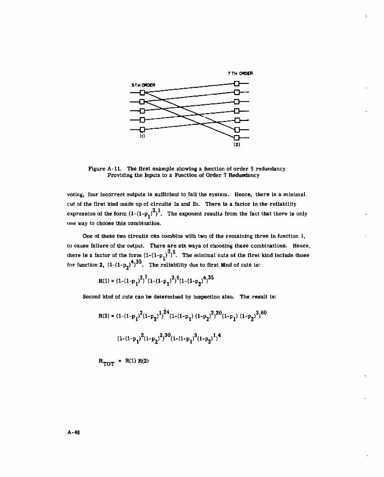
7 TH ORDER
?5TH ORDER
(2)
Figure A-11. The first example showing a function of order 5 redundancyProviding the Inputs to a Function of Order 7 Redundancy
voting, four incorrect outputs is sufficient to fail the system. Hence, there is a minimal
cut of the first kind made up of circuits la and lb. There is a factor in the reliability
expression of the form (1-(1-p 1 )2 )1 . The exponent results from the fact that there is only
one way to choose this combination.
One of these two circuits can combine with two of the remaining three in function 1,
to cause failure of the output. There are six ways of choosing these combinations. Hence,3 6there is a factor of the form (1-(l-pl)3)6. The minimal cuts of the first kind include those
for function 2, (1-(l-p 2)4)35. The reliability due to first kind of cuts is:
R(l) = (1-(l-p)2)l (l-(1-Pl) 3 )6(l-(l-p 2 )4 )3 5
Second kind of cuts can be determined by inspection also. The result is:
R(2) = (1-(1-Pl)2(1-p2)I)24(1-(1-Pl) (1-P2)2)20(1-Pl1 (1-P2)3)60
2 230 3 14
(1-(1-P 1I) 2(1-P 2 ) 2) 30(1-(1-PI ) 3(1-P 2) 1)4
RTOT = R(l) R(2)
A-48

9TH ORDER
Figure A-12. Example Showing A Function of Order 5 redundancy providing the inputsto A Function of Order 7 Redundancy
This example shows how different the parameters can be for a similar case. In this
case there are four circuits in function 1 each feeding two circuits in function 2,and only
1 which feeds one circuit in function 2. There is no longer a case where failure of less
than a majority of circuits in function 1 can shut the system down, as in the first example.
When the orders of redundancy are changed further, there is little generality in the minimal
cut relationships. This reliability due to the first kind of cuts for this example is:
R(1) = (1-(1-Pl)3)4(1-(-Pl) 3)6 (-(1-P25)126
That for the second kind of cuts is:
R(2) = (1-(1-pI) (1-p2)3)140 2(1-P 1)2(loP2)1)30(1- (4-p1) (1-P2)4)70
(1-(1-P1)2 (-P2))60
In short, it is possible to determine the minimal cuts and, thereby, the reliability
for given networks. However, it has been found to be prohibitively difficult to generalize
these expressions for functions of any two orders of redundancy.
A-49/50
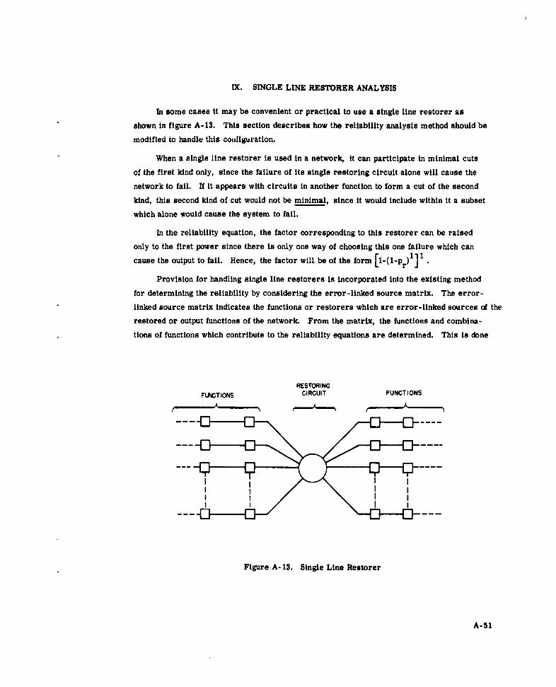
IX. SINGLE LINE RESTORER ANALYSIS
In some cases it may be convenient or practical to use a single line restorer as
shown in figure A-13. This section describes how the reliability analysis method should be
modified to handle this configuration.
When a single line restorer is used in a network, it can participate in minimal cuts
of the first kind only, since the failure of its single restoring circuit alone will cause the
network to fail. If it appears with circuits in another function to form a cut of the second
kind, this second kind of cut would not be minimal, since it would include within it a subset
which alone would cause the system to fail.
In the reliability equation, the factor corresponding to this restorer can be raised
only to the first power since there is only one way of choosing this one failure which can
cause the output to fail. Hence, the factor will be of the form [--(1-Pr)l] 1 .
Provision for handling single line restorers is incorporated into the existing method
for determining the reliability by considering the error-linked source matrix. The error-linked source matrix indicates the functions or restorers which are error-linked sources of the
restored or output functions of the network. From the matrix, the functions and combina-
tions of functions which contribute to the reliability equations are determined. This is done
RESTORINGFUNCTIONS CIRCUIT FUNCTIONS
Figure A-13. Single Line Restorer
A-51

by identifying the functions and restorers which are present and placing these in the reli-
ability expre~sion-for.first idd of minimal cuts. Then taking combinations of two functions
and restorers and placing these in the reliability equation for second kind of cuts, etc.
Since a single line restorer participates only in first kind of minimal cuts, it should not
be considered in cuts of the second and higher kinds, hence, after the reliability for the
first kind of minimal cut has been calculated the columns representing these single line
restorers should be all changed to all O's. They, then will not enter into the equations of
higher kind.
A-52

X. PROGRAM FOR COMPUTING THE RELIABILITY OF REDUNDANT SYSTEMS
The analysis of redundant systems has progressed to the point where it is desirable,
even imperative, that there be some fast and accurate technique for determining the reliabili-
ty of these systems.
This need has grown from the development of a technique for synthesizing complex
networks for high reliability. This technique requires accurate calculation and comparison
of reliabilities for many different arrangements of functions and restorers. Further, present
methods are unable to readily handle the complex expressions which describe the reliability
of a system. Often, inaccuracy results in the processes of multiplication and exponentiation
due to values of circuit reliability which often very closely approach the value 1 (i. e. 0. 9999).
To eliminate these problems, a program is being developed which will implement
these calculations. The general outline which the program follows will be discussed here.
A. GENERATING THE ERROR-LINKED SOURCE MATRIX
The input data for a given reliability calculation will consist of a) the functions present,
b) location of restorers, c) primary error-linked sources to each function, d) output
functions, and e) the probabilities of correct operation assigned to each circuit of the
functions and restorers. From this input data, the computer will generate the primary
matrix. This will be done by entering l's in the elements of the matrix for the functions
present and their primary sources and a 0 for every other element in the matrix. This
yields the primary matrix without restorers.
In order to include the effect of the restorers on the system, it is necessary to
modify the primary matrix without restorers. This is done by first indicating the presence
of the restorers. Then, since a restorer takes onall the outputs of its restored function,
it is necessary to switch to these restorers the outputs of the functions which they restore.
When a function is indicated as a restored function, the computer will remove all the
ones in the column corresponding to that function except that on the principal diagonal, and
place them in the corresponding rows in the column which describes the restorer. A one
will be placed in the column assigned to the restorer on the principal diagonal also, to
denote the presence of the restorer in the circuit. Once every restorer has been placed
in the matrix and all the outputs shifted, the primary matrix has been completed.
In order to arrive at the composite matrix, successive matrix multiplications must
be performed. The secondary matrix is found by a multiplication of the primary matrix by
itself. The computer performs this process in the following manner. The X column,
A-53

Y row element for the secondary matrix is found by taking the product between corresponding
elements of the Y row and X column of the primary matrix and performing a Boolean summa-tion of these products. A corresponding procedure is performed for each element in the sec-ondary matrix. This process can be done easily by the computer by using scanning techniques.The computer scans the Y row and the X column and compares the location of the l's. If a
correspondence is found, a 1 is placed in the secondary matrix in the element for which we aretesting, (Y, X) element. If no correspondence is found, a 0 is placed in that element of the
secondary matrix. Because the process calls for a Boolean summation of the products, only
one correspondence need be found. This is done for all elements of the secondary matrix.
Once the secondary matrix is found, it is checked for every element, against the
primary matrix. If correspondence is found in every element, the secondary matrix is
the composite matrix. If there is at least one difference between the two, another matrix
multiplication is performed and another check is made. This process continues until a
correspondence is found. The final matrix, the one which corresponds to the previous one,
is the composite matrix.
The program will call for a count of the number of matrix multiplications performed
in order to yield a value for the highest order input source present in the network.
Once the composite matrix has been found, it is reduced to the error-linked source
matrix by extracting those rows which correspond to the restored functions and output
functions, the locations of which are given information.
B. CALCULATING THE RELIABILITY OF A SYSTEM
From the information contained in the error-linked source matrix, it is now oossible
to compute the reliability of the system. The total reliability is calculated in several
parts; that due to first kind of cuts, that due to second kind, third kind, etc. The finalsystem reliability is the product of the individual reliabilities of the different kinds of
minimal cuts.
Since the equations for the probability that the system does not fail due to first,
second, and higher kinds of minimal cuts have already been developed in Section V of this
Appendix, it becomes necessary for the computer only to identify the functions and combi-
nations of functions which make up these minimal cuts, and then to solve the equations.
A-54

1. Identifying the Minimal Cuts
a. First Kind of Minimal Cuts
A function or restorer introduces minimal cuts of the first kind whenever
it is present in the system. Therefore, the computer needs only to identify whether functions
or restorers are present in the system in order to identify minimal cuts of the first kind.
This is done by scanning the columns, and, if a one appears in a column, the conputer
calculates the probability that the system will not fail due to a first kind of cut in this func-
tion. The expression for this probability has already been developed, and it remains only
to calculate it. Since a function appears only once in the system, its probability of failure
because of a first kind of cut should not be taken into account more than once. Therefore,
whenever a 1 is found in a given column, the computer shifts to the next column and con-
tinues the search. The product of the probabilities for each of these functions and restorers
is the probability that the system will not fail due to a minimal cut of the first kind.
b. Second Kind of Minimal Cuts
Second kind of minimal cuts consist of circuits in either a restored function
and one of its error-linked sources or two error-linked sources of the same restored
function. Since a row of the error-linked source matrix indicates a restored function and
all its error-linked sources, any combination of two l's in a row of the matrix will form
a combination which can have circuit failures which will make up a minimal cut of the
second kind. The computer, then, in a given row of the matrix, locates the first 1 and
holds its position in memory. It then scans until it finds another 1. This, tngether with
the 1 in the memory describes the first combination of functions that can appear together
in the same minimal cut. It then scans down the row until it finds the next 1, etc. After
all the combinations of the first one with other l's are completed, the computer memory
shifts from the first 1 to the second 1 and the process repeats. This continues until all
possible combination of two l's on a given row have been found. The computer then moves
on to the next row. On each succeeding row, whenever a combination of two l's is found,
the computer checks back to preceding rows to see if this combination has been found
before. If not, the formula for second kind of cuts is used and a probability of not failing
due to a second kind of cut in the two functions selected is computed for each combination
found.
c. Third and Higher Kinds of Cuts
For third kinds of minimal cuts, the same process as for second is
repeated except combinations of three ones on a given row are found; for fourth kind,
A-55

combinations of four, etc. For each kind of minimal cut, a probability is found that failure
due to that kind of minimal cut will not result. The system reliability is the product of
these probabilities for the different kinds of minimal cuts.
In an order m system, the highest kind of minimal cut which can occur is
m-k+l, in which case there would be onie circuit failure in each of m-k+l functions. After
the (m-k+1) th kind of cut has been calculated, the computer will stop finding combinations.
2. Computation of Reliability
In the reliability equations for each kind of cut there will be factors of the form
[l-(1-p)n] m . Since p is a number close to 1, the term (l-p) n will be very small, and
when subtracted from one, leaves a number close to one to be raised to a large power.
This may lead to loss of accuracy due to rounding off and limitations on the word size in the
computer; and, when a series of these numbers is multiplied together, still further loss
of accuracy results. In order to remove this loss of accuracy, several measures have
been taken. To raise this factor to the power m, an expansion approximation will be used,
and all calculations will br, made using complements as opposed to the numbers themselves.
To multiply the two factors (l-(1-Pl)nl)m (1-P2)n2)m2 together, the terms
(1Pl)nl and (1-P 2)n2 will be calculated and put in floating point notation. This leaves the
expression in the form (1- £1)ml (1- £2 )m2 where E = (1-Pl)nl and £2 = (1-P2)n2
Now the approximation is employed. (1- 1)ml =
1-m 1 E1+ 1/2 ml(ml-1)E12 -1/3 mI(m 1-1) (m1-2)E 1
3 + .
This will be carried out until single precision accuracy is no longer affected. This changes
the expression to the form (1 - a1) (1 - a 2) where:
0-1 = M I E - 1/2 mn I(m- 1) F12 + ....
'2 m2 '2- 1/2 m2 (m 2 - 1 ) f22 +
This product can be written as 1- 0-, - o2 + - 0" or 1 - (or1 +°r2 -0-1 02
The new expression for this product is now (1- 0-12)
where a12 =a + °" 1 r 2
A-56

The form (1- o* however, can't be held by the computer without actually
working out the subtraction, hence, rather than lose the accuracy, the program will compute
from this point in complements, i.e., it will not proceed as far as the (I -a ) form. Rather
it will solve for o- and o'2, then a 12" It will then move on to the next factor, compute -3
and combine this value with o-12, in the same manner as a- and a 2 were combined, to
form a 12 3 . This will continue until the final a"123..". has been attained.
This will still be contained in floating point form and will be the complement
of the reliability of the expression calculated. This will be printed out along with the
reliability itself. Thus if rounding off occurs in the subtraction the answer, accurate to
more than single precision, will be retained.
A-57/58

TABLE OF CONTENTS
Section Page
I THE SET OF ISOLATED REGIONS AND THE CORRESPONDINGLIST OF ISOLATING ARRAYS FOf A SINGLE FUNCTION ....... ... B-2
nI RULES FOR GENERATING THE LIST OF ALL ISOLATINGARRAYS OF THE FIRST FUNCTION ..... ................ ... B-il
III THE ISOLATING ARRAYS OF A GROUP OF FUNCTIONS .... ........ B-13
IV GENERATION OF THE ISOLATING ARRAYS OF THE EXAMPLENETWORK OF FIGURE 4-5 ....... .................... B-15
LIST OF ILLUSTRATIONS
Figure PageB-i Network Used to Describe the Procedure for Generating the
List of Isolating Arrays ....... ..................... ... B-1
B-2 The Sources of Function 1 .......... ..................... B-2
B-3 Regions Which Include Only Error-Linked Sources of Function I . . .. B-4
B-4 Expanding a Region Generated in the First Step to Include Sinksof Functioni.... . . .. . . . . ...................... ... B-5
B-5 Expanding a Region to Include the Primary Sinks of Function 1and Their Sources ........ ........................ ... B-6
B-6 Functions That May Be Added to the Region by the SecondApplication of the Second Step of the Procedure ..... ........... B-7
B-7 Expanding the Region to Include Secondary Sinks of Function 1 ....... B-8
B-8 Isolated Region of Function 1, from the Network of Figure B-i,in Which Location 2 is Empty ...... ................... ... B-14
B-9 The Functions Which must be Considered in the Isolated Region ofFunctions 1 and 2 ........... ........................ B-14
B-10 Example Network with its Primary Source Matrix ............. .... B-15
~B-i/ii

APPENDIX B
GENERATING THE ISOLATING ARRAYS
A vital companion to the synthesis procedure is the ability to compile a list of all the
isolating arrays of a function or group of functions. This appendix shows how this list is
generated, first for a single function and then for a group of functions. The procedure is
used to generate the complete list of arrays for the example in the "Detailed Procedure" por-
tion of the text.
An isolated region is defined for a set of functions, A, such that every function or re-
storer in the region is error-linked to one of the functions in the set A, when all the locations
of the set are empty. Every function not in the region is isolated from every member of the
set. The locations of the set A take on various states during the synthesis procedure. In
Section IV. B. 4., they assume the states "0" and "? ", but for the purpose of generating the
isolated regions, they are set equal to 0. For every isolated region there is one and only
one isolating array. The only locations specified in the isolating array are those that are
necessary to define the contents of the isolated region or the restorers on its boundaries.
This study has investigated a number of techniques for generating the list of isolating
arrays, and this appendix describes one of them. The rules for generating the list are de-
scribed primarily by example. The network used in the discussion appears in figure B-1.
The functions in this example are numbered in accordance with the rule in Section IV. B. 4.
13 12 1 1iB 14
6 017 19 20
Figure B-1. Network Used to Describe the Procedurefor Generating the List of Isolating Arrays
B-1

I. THE SET OF ISOLATED REGIONS AND THE CORRESPONDING LISTOF ISOLATING ARRAYS FOR A SINGLE FUNCTION
The first requirement of the synthesis procedure is a list of isolating arrays of function
1. The scheme for generating this list is described in this section.
For a function to be in an isolated region of function 1, it must be error-linked with the
function 1. Then the function must bear at least one of three relationships to the first func-
tion. It must be:
1. an error-linked source of function 1,2. an error-linked sink of function 1,
3. an error-linked source of an error-linked sink of function 1.
The list of regions and arrays is compiled in two steps. The first step finds all theregions which include the first function and functions that fall in the first classification. Each
of the arrays generated in the first step are subjected to repeated application of the second
step to add the functions which fall into the second and third classification.
The functions which are sources of function 1 are shaded in figure B-2. Functions not numbered
can be identified by their position in the network and comparison with figure B-1. The first
step in the procedure finds all the sets of the shaded functions which fulfill the requirements
of an isolated region. The step begins with the smallest of all regions which includes function
4
SOURCES Of FUNCTION I
Figure B-2. The Sources of Function 1
B-2

1 and function 1 alone. The region will be expanded in size from this small beginning, and
locations through which the region can be expanded to include primary sources of function 1
are given the state 0. For this example, the only location that have this quality are locations
2 and 3. Locations through which the region can be expanded into the sinks of function 1 are
given the statc 6. This expansion iR carried out in a step described later. The region con-
sisting of only function 1 is shown with its array in figure B-3. a.
All the arrays are to be enumerated so the region is allowed to expand in all possible
ways from function 1. Allowing the O's to assume all possible states accomplishes this.
When a location (0) assumes the 0 state, its function is addedto the region, ,and avenues for
expansion into the secondary sources of function 1 are now available, through the locations of
the primary sources of these last added functions. These locations assume the state 0.
When the location takes on the 1 state, further expansion through that location is re-
stricted; hence, no new O's are added. In figure B-3. b, the 0'd locations of figure B-3. a
have taken on all possible states.
The arrays representing a region are shown below the illustration of the region.
The regions generated in figure B-3. b are now expanded through their O'd locations.
Note the region consisting entirely of function 1 and restorers 22 and 23 cannot expand at this
step because the restorers have cut off all paths to other sources of function 1. There are no
0's in its array. The O's in the other regions in figure B-3. b are allowed to assume all pos-
sible states in figure B-3. c. No new 0 locations are introduced in this step because the in-
puts of the network have been reached.
When there are no regions with 0 locations that have not been allowed to assume all
states, all regions consisting of function 1 and its error-linked sources have been enumer-
ated. Only regions without 0's need be retained. The regions which include 0 locations are
intermediate results of this step and can be discarded as the O's are allowed to vary. The
underlined arrays in figure B-3. b and B-3. c are kept for the next step in the procedure.
The next step, in the procedure, is to allow each of the regions generated in the first
step to expand into the primary sinks of function 1. These are functions 7 and 8, for the
example, which are shown in figure B-4 as black boxes. Note that one of the regions gener-
ated in the first step is shown in this figure. This step must be performed for all regions
so generated.
Because the isolated region is defined for location 1 empty, then 8 is only allowed to
assume the 0 state. New avenues to other sinks of function 1 are opened through the new
members of the region so their locations take on the 8 state as shown in figure B-5b.
B-3

71.71
8Oistxxxxxxxxxxxx~x )
11OXgXXXuXaXXXX ) (X 60OIIIXxxxxKxxxKxxx )
(SIxo1x1xmxxxxx) boogxugxxzaxxx
(9,xe1xzxxxxxxx)(Sogoxxxxxxxxxzx
SwOOXIxxaxxuuxxxxxxx)xxx
(84OXCOXiXXXXX)80lxxxxxxxxxxx)Coorxxxxaxxxxx
(Sooxxxxxuxxxx,.x)
(E01ox7Exxxx)x
(B7DgAD
Figure B-3. Regions which include only Error-Linked Sourcesof Function 1
B-A

13 12 1
24 21
* OUTPUT SINKS OF FUNCTION I
INPUT SOURCES OF THE OUTPUT SINKS OF FUNCTION I
Figure B-4. Expanding a Region Generated in the First Stepto Include Sinks of Function 1
Functions which are sources of these newly added sinks can also be error-linked to
function 1, so the locations of the primary sources of these functions should be made 0 if
they have not already assumed the 1 or 0 state in the region. This is also shown in figure
B-5. b.
The region of figure B-5. b is now expanded to include more and more sources of the
primary sinks of function 1 by allowing the O's to take on all states just as in the first step
of the procedure. These sources are shown shaded in figure B-4. The process is started in
figure B-5. c. It continues until there are no regions which include 0'd locations.
Each of the regions generated in the first step must be subjected to the second step
of the procedure. At the end of this step, a number of different regions have been generated
- each with 8 's on locations 7 and 8, and non with 0's.
The second step is now reapplied to every region including 8 locations to expand the
region Into the secondary sinks of function 1. The S 's In each region assume all possible
states. When the 9 becomes 0, new sinks are added to the region. If they are sources of
other functions, the locations of these new sinks assume the S state. When the S becomes
1, a restorer is placed in the location and the region is restricted from further expansion
B-5

O - 0
0
en
eGo
OD X
X
GO X
( CD r- X-
CIO x X 0O
N GO
NX ItG
0l 0 w 0 d
N N
N 4
B 0 0
In -
M GOXX
0
GO0G10
00 4
'C''C
Nj ''C'C'C'C'C
0 0
Figure B-5. Expanding a Region to include the Primary Sinksof Function 1 and their Sources
B-6

into other sinks of function 1 through the location. When the sinks are added, avenues are
opened for expansion of the region into the sources of the newly added sinks. The locations of
these sources take on the state 0.
Figure B-6 shows onc region generated in the second step. The sinks into which the
region may expand are shown in black, and their sources are shown shaded. In this reappli-
cation of the second step, all regions that include these functions are generated. This step
must be performed for every region generated when the second step was first applied.
31 8 14
SINKS OF FUNCTION ?OR8
SOURCES OF FUNCTION 15
Figure B-6. Functions that may be added to the Region by theSecond Application of the Second Step of the Procedure
In figure B-7, the 8 's in one of the regions generated in the first application of the
second step of the procedure are allowed to assume all possible states. Where new avenues
are introduced for expansion of the region into the sources of the newly added functions, the
locations through which the expansion will occur are indicated with a 0. The O's are treated
in the same manner as before. The regions which are generated with no locations having the
states 0 or 6 are the desired products of the procedure, isolated regions. Their associated
arrays are, of course, isolating arrays.
B-'7

4
(0011 I IOI X I XXOXXX X )
(00111 xIOI I XXOOXXXXX)
(0031x008 280 14x
Fiur B-.EpnigteRgo2oicud eodr ik fFnto
B-B]
71

When both locations 7 and 8 are filled as in one of the regions of figure B-7, the re-
storers 27 and 28 are not error-linked to function 1; but, they are necessary to the formation
of the isolated region. They do not appear in the region, but they must be specified in the
isolating array identifying the region.
In some of the arrays of figure B-7, locations 14 and/or 15 are specified as 0. This is
because these functions are network outputs and are assumed restored. Therefore, it is un-
necessary to investigate the case of restorers in these locations.
The second step should be accomplished for each of the arrays which include 6 's. For
this example, the step will be carried out once to every array generated in the first applica-
tion of the second step, and all the isolated regions and their arrays will have been generated.
In general, the step should be applied to every array with locations specified as 6 , until no
arrays with 6 's or O's remain in the list. Then the list of all isolating arrays of function 1
will have been generated.
B-9/10
H. RULES FOR GENERATING THE LIST OF ALL THE ISOLATING ARRAYSOF THE FIRST FUNCTION
Iu Uie description of the generation of isolating arrays, it was required that there be no
O's in the arrays of the list when the 6 locations are allowed to vary. This restriction is really
unnecessary as the order in which functions are added to an isolated region makes no dif-
ference to the final content of the region. The expansion of the regions to include sources
or sinks can be carried out in any desired order. Also, it is unnecessary to draw regions
to generate the list of arrays. This was done primarily to aid the reader to visualize the
steps of the procedure.
Five rules are sufficient to describe the complete procedure for the generation of the
list of isolating arrays. The careful application of these rules will result in the desired
list.
Rules
1. Start with an array in which the state of the first location is S , and the
states of the locations of its primary sources are 0. The primary sources
of the first function are found in the primary matrix of the network without
restorers. The primary matrix is described in Section IV. A. 2 of Appen-
dix A.
2. For any array in the list which includes 0's, let the states of the locations
which are 0'assume all possible combinations of values. Since each location
takes on two states if there are k locations in state 0, there will be 2k com-
binations of states of the k locations.
When a location assumes the state 1, the array does not change.
When a location assumes the state 0, its function joins the region. The lo-
cations of this function's primary sources now take on the state 0 if they
are not already specified as a 1, 0, or 6 .
After applying this step to an array, the array is discarded.
3. Let S locations in any vector assume all possible states.
When a location takes on the 1 state, the array does not change.
When a location takes on the state 0, the primary sinks of its function are
added to the region so their locations assume the state S , if they are not
already specified as 1, 0, or 9. The primary sources of the last added
B-il

functions assume the state 0 if they are not already specified as 1, 0, or
S . After applying this step to an array, the array is discarded.
4. When an array contains neither O's nor S 's, an isolating array has been
generated. This vector can be placed in a separate list of isolating arrays.
5. Apply steps 2 and 3 to vectors in the list which contains O's and 6's until
therp are no such vectors remaining, and all the isolating arrays have been
generated. It is not necessary to order the application of steps 2 and 3 in
any way.
B-12

I. THE ISOLATING ARRAYS OF A GROUP OF FUNCTIONS
The isolating arrays of a group of functions, say functions I to h, can be found from
the list of isolating arrays of the smaller group of functions, 1 to h. 1. The relationship be-
tween the two lists depends on whethet function h is a primary source of a primary sink of one
of the functions in the group 1 to h-1. The system of numbering functions in the network re-
quires it to be one of these.
Say that function h is a primary sink of function -e , where e < h. An example of this
relationship is in figure B-1. Here function 7 is a sink of function 1. Now assume that all
the isolating arrays of functions 1 to h-i are known. By definition, every function in the
region specified by an array must be error-linked to at least one of the functions 1 to h-i
when locations 1 to h-1 are empty. Consider an isolating array in which location h is empty.
Because h is a primary sink of function X when locations h and .e are empty, all the functions
that are error-linked to function h must also be error-linked to function 4 . Then the ad-
dition of function h to the group of functions introduces no new functions into the region, and
the isolated region of functions 1 to h-i is also an isolated region of functions 1 to h. In
general, if finction h is a primary sink of a function t which is in the group 1 to h-i, the
isolating arrays of function 1 to h-i in which location h is 0 are also isolating arrays of func-
tions 1 to h.
If function h is a primary source of function , c< h, but a primary sink of no other
function in the group, the addition of function h to the group may add new functions to an iso-
lated region. For example, in figure B-i, function 2 is a primary sink of function 1. Con-
sider an isolated region of function 1 to h-i in which location h is empty. Because h is an
error-linked source of e , all the error-linked sources of h are also error-linked sources
of -e . There may be sinks of function h or sources of these sinks, however, which are
error-linked to h but not to any of the group 1 to h-i. When h is added to the group, new
regions must be generated which include these new functions. For instance, consider the
isolated region of function 1 shown in figure B-8. All the functions and restorers in this
region are errL:.-linked with function 1. Now when forming the isolated regions of both
functions 1 and 2, the sinks and the sources of the sinks of function 2 must also be considered for
expansion of the region. These functions are shown dotted in figure B-9.
In general, to account for these functions, for every isolating array of functions 1 to
h-1 in which location h is empty, let all the unspecified primary sink locations of function h
assume the state S and let the unspecified primary sources of these sinks assume the
state. Them proceed with the isolating array generation as in part A of this appendix.
B-13

(0011 IXI IX IXXXXXXXXX)
Figure B-8. Isolated Region of Function 1 from the Network of Figure B-1in which Location 2 is Empty
L__-i iL_-I L--I
Figure B-9. The Functions which must be Considered in the Isolated Regionsof Functions 1 and 2
For the example of figure B-9, the locations of the primary sinks of functions 2, loca-
tions 11 and 1, are already specified, so no S's are added to the array. The location of a
primary source of function 11, location 12, is not specified in the array, so it assumes the
0 state. Application of the array generating procedure will provide the isolating arrays of
functions 1 and 2.
B- 14

IV. GENERATION OF THE ISOLATING ARRAYSOF THE EXAMPLE NETWORKOF FIGURE 4-5
The example used in the text, Section IV. B. 4., to describe the detailed synthesis pro-
cedure requires that all the isolating arrays of function 1 be known. This section derives
these arrays in accordance with the rules of Section I of this appendix. The network with
its primary source matrix are shown in figure B-10.
~110000
011010
001101
100010
000011
Figure B- 10. Example Network with its Primary Source Matrix
Table B-i shows the generation of isolating arrays. The underlined arrays are isolatingarrays. Location 4 is set 1o 0 in all arrays since it is an output function. This is discussed
in IV. C. 4.
Table B-1. Generation of the Isolating Arrays of the Example Network
Number Array From Array
1. (SXXOXX) 1
2. (osxo8X) 2
3. (O1XO1X) 2
4. (00801 X) 2
5. (01800 ) 2
6. (00800) 2
7. (O0101X) 4
8. (000010) 4
9. (000011) 8
10. (000010) 8
11. (011001) 5
12. (010001) 5
13. (011000) 5
14. (010000) 5
B,-15

Table B-1. Generation of the Isolating Arrays of the Example Network (Continued)
Number Array From Array
15. (001001) 6
16. (00000) 6
17. (001000) 6
18. (000000) 6
B- 16

APPENDIX C
GENERATING THE ISOLATED REGIONS FROM THE ISOLATING ARRAYS
Once the isolating arrays of a network are determined, it remains to calculate the cost
of the isolated region determined by each isolating array in order to arrive at the least ex-
pensive system - the optimum system. To find the cost of the isolated region, it is necessary
to calculate the reliability of the region, since this is an important consideration in determin-
ing cost. With present methods of computing reliability, the functions in the region and the
connections between them must be known. This section will deal with a method for finding the
configuration of the isolated region for a given isolating array.
Two functions are isolated from one another when a failure in one cannot combine with
a failure in the other to cause system failure. This technique utilizes the concept of error-
linked functions to determine the form of the isolated region. To review the definition in
Section III. C. 1, two functions are error-lirked when:
1) one is a source or sink of the other and there is an unrestored path be-
tween them.
2) They are both sources of a third function, and there is an unrestored
path from each to this third function.
In an isolated region, all functions are error-linked to the function whose location is
being optimized. Any function which is not error-linked to this function is outside the iso-
lated region. Hence, to identify an isolated region of a function, it is necessary only to
identify all the functions which are error-linked to this function.
This method will first locate all those sources and sinks of the location to be optimized
which have unrestored paths between them and the function under optimization. This will
locate all those functions which fulfill the first error-link criterion. Then, every source of
each sink located in the previous step which has an unrestored path to this sink is located.
This identifies those functions which fulfill the second error-linking criterion. These two
procedures identify all the functions in the isolated region.
The isolating array describes the location of restorers in a network. The connection
matrix, which is the same as the primary matrix with the l's on the main diagonal removed,
describes the form of the network by illustrating, in matrix form, the primary sources and
sinks of each function. Together, these two tools contain all the information necessary to
describe the isolated region, indivisible isolated region(s) and unspecified regions. With
them, it is possible to derive the form of the region described by the particular isolating
array.
C-1

An example will be considered here to clarify the discussion. The example and its
connection matrix are shown in figure C-1. A sample isolating array is chosen (0, 0, 1, X, 1, 1).
0 01 Xii
1 000000 0
2 1 00 00 023
3 0100 10
4 0010 01
5 100000
6 0000 10
123456
Figure C-1. Example Network with its Connection Matrix
In the connection matrix, the vertical columns represent the primary sinks of the func-
tion (i. e., function 1 has sinks 2 and 5). The rows indicate the primary sources of a function
(i. e. function 3 has sources 2 and 5).
In seeking the isolated region for the chosen isolating array of the first function, the
first function is the starting point:
The isolating array, column 1, shows no restorers present in location 1. In this case,
the output sinks of location 1 and the input sources of these output sinks are added. The sinks
are found as l's in column 1 of the connection matrix. There are no input sources of these
sinks other than function 1. This is determined by the fact that there are no other l's in the
rows in which the l's of column 1 are located.
The isolated region expands to: 2
Now locations 2 and 5 are investigated. Location 2 has no restorer present, thus its
output sinks and any input sources they might have are added; location 5 is restored. The
restorer on location 5 is an input source of function 3 and is, therefore, added. The pro-
cess is terminated for function 5.
C-2

Location 3 is restored so the process ends. This is the isolated region of location 1
for the array shown.
Since indivisible isolated regions must be calculated separately, then added to other
costs to arrive at a total cost, these inust te Identifiable. An indivisible is'lated region
can have no members which are error-linked to any function outside this region. An indivi-
sible isolated region can be recognized with the use of the isolating arrays and the connection
matrix. After the functions in the isolated region have been identified with the procedure of
the last section, all the members of this region are now tested to determine if all their sources
(rows of the matrix) and sinks (columns of the matrix) are in the region. If none of these
functions in the isolated region is error-linked to functions which are outside the isolated
region, the region is an indivisible isolated rerion and its cost may be calculated separately
and added to the cost of the rest of the network to arrive at the network cost. If such error-
linkages do exist, this is not an indivisible isolated region and its cost may not be added to
other costs for total network costs.
C-3/4
REFERENCES
1. Mann, W. C., "Systematically Introduced Redundancy in Logical Systems",
1961 IRE International Cony. Rec. 9, Pt. 2, 241-263 (March, 1961)
2. Jensen, P. A., "Four Redundant Configurations", Westinghouse Electric Corp.,
Electronics Div., Advanced Development, Dec. 1, 1961, (Rept. No. EE-2600)
3. McReynolds, J., "Evaluation of the Majority Principle as a Technique for Improving
Digital System Reliability", Hycon Eastern, Inc., July 8, 1958, (HEI Publ. No.
M-577) First Annual Report for Contract NONR-2133(00)
4. Esary, J. D. and F. Proschan, "The Reliability of Coherent Systems", Redundancy
Techniques for Computing Systems, Ed. by R. H. Wildox and W. C. Mann, Sparton
Book, Wash., D. C., 1962 (pp 47-61)
5. Esary, J. D. and F. Proschan, "Coherent Structures of Non-Identical Components",
Boeing Scientific Res. Labs., Feb. 1962, (Math. Note No. 251)
6. Ledley, R. S., Digital Computer and Control Engineering, McGraw Hill, 1960.
R-1