60

4. EVAPORATION 4.1 Basic Concepts and Definitions in Boundary-Layer Meteorology Since evaporation is a meteorological phenomenon, we need to be familiar with some terminology in boundary-layer meteorology. Air is seen as a mixture of “dry air” and water vapor. We use d to indicate density (kg m-3) of dry air and v for the density of water vapor in this chapter.

→ see Brutsaert (2005, p. 24) By definition, the “bulk” density of moist air is = d + v (4-1) The mixing ratio (m) is defined as m = v/d (4-2) The specific humidity (q) is defined as the mass of vapor contained in the unit mass of moist air:

m

mq

dvdd

dv

vd

vv

1//

/

(4-3)

Since m is much smaller than 1, q ≅ m (4-4) The ideal gas law is written as:

TR

V

np i

i *

where pi is the pressure (Pa) of component i in the gas mixture V (m3) is the volume of the gas mixture ni (mol) is the mass of component i in the mixture R* (= 8.3144 J mol-1 K-1) is the universal gas constant T (K) is temperature The ideal gas law can be also written:

TRT

w

RT

w

R

V

MTR

w

M

Vp ii

ii

i

i

i

ii **

*1000

001.0001.0

1 (4-5)

where Mi is the mass (kg) of the gas wi is molecular mass (g mol-1) Ri (= 1000R* / wi) is the specific gas constant (J kg-1 K-1). The wd for dry air is 28.966 g mol-1 and ww for water is 18.016 g mol-1.

Rd = 287.04 J kg-1 K-1 and Rw = 461.5 J kg-1 K-1. Assuming that air consists only of dry gas and vapor,

p = pd + e

61

where p is total air pressure pd is the partial pressure of dry gas e is the partial pressure of water vapor From Eq. (4-5),

TR

ep

TR

p

dd

dd

(4-6)

TR

e

TR

e

dwv

622.0 (4-7)

Note that 622.0016.18

966.28 dd

w

ddw

RR

w

wRR

From Eqs. (4-6) and (4-7),

p

e

TR

peep

TR ddvd 378.01622.0

1

p

ep

e

p

e

TR

p

TR

e

q

d

dv

378.01

1622.0

378.01

622.0

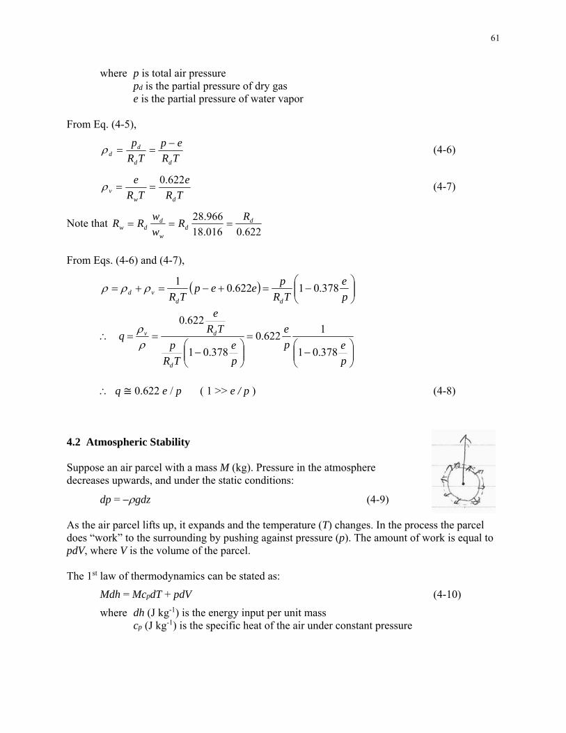
q ≅ 0.622 e / p ( 1 >> e / p ) (4-8) 4.2 Atmospheric Stability Suppose an air parcel with a mass M (kg). Pressure in the atmosphere decreases upwards, and under the static conditions:

dp = gdz (4-9) As the air parcel lifts up, it expands and the temperature (T) changes. In the process the parcel does “work” to the surrounding by pushing against pressure (p). The amount of work is equal to pdV, where V is the volume of the parcel. The 1st law of thermodynamics can be stated as:

Mdh = McpdT + pdV (4-10)

where dh (J kg-1) is the energy input per unit mass cp (J kg-1) is the specific heat of the air under constant pressure

62

Note that the first term on the right hand side represents the internal energy change due to temperature only (fixed pressure), and the second term represents the work under constant temperature. Under the constant temperature, the ideal gas law requires:

pV = constant → d(pV) = 0

But from calculus:

d(pV) = pdV + Vdp = 0

pdV = Vdp Substituting this into Eq. (4-10) gives:

Mdh = McpdT – Vdp

dh = cpdT – (1 /) dp since = M / V Substituting Eq. (4-9) into this gives (see Brutsaert, p.29, Eq. 2.21):

dh = cpdT + gdz (4-11)

(1) Partially saturated air The saturation vapor pressure (e*) is a function of temperature (see Brutsaert, p. 28). Let’s consider the case, where e is sufficiently smaller than e* so that the condensation of liquid water does not occur in the air parcel. If the parcel rises quickly enough so that the energy exchange is negligible, then dh = 0 in Eq. (4-11).

pc

g

dz

dT (4-12)

The magnitude of the gradient in Eq. (4-12) is called the dry adiabatic lapse rate (d). Since cp ≅ cpd = 1005 J kg-1 K-1 at 273.15 K (Brutsaert, p. 25), d = g / cp = (9.81 m s-2) / (1005 J kg-1 K-1) = 9.8 × 10-3 K m-1 = 9.8 K km-1

If the actual dz

dT is greater than d, then the rising air parcel

cools down at a rate slower than .

→ The temperature of the parcel is higher and the density ( 1/T from the ideal gas law) lower than the surrounding.

The air parcel keeps rising.

Therefore, > d indicates the unstable condition.

63

If < d, then the rising air parcel gets cooler and denser than the surrounding.

→ It stops rising.

< d indicates the stable condition. In the neutral atmosphere ( = d), the temperature of the rising parcel is always equal to the surrounding. This serves as a reference for analyzing atmospheric processes. Therefore, meteorologists define potential temperature, (K) as “the temperature that would result if an air parcel at an arbitrary height was brought adiabatically (dh = 0) to a standard pressure level (i.e. altitude) of p0 = 1000 hPa”. To define mathematically, we note (see page 62):

dh = cpdT – (1/)dp

But TR

p

RT

p

d

p

TRd1

For dh = 0,

dp

p

TRdTc dp

p

dp

c

R

T

dT

p

d

Integrating this from (T0, p0) to (T, p),

p

pp

dT

T

d

c

Rd

00

00

lnlnp

p

c

R

T

T

p

d

p

d

c

R

p

p

T

T

00

p

d

c

R

p

pTT

0

0 where Rd /cp = 287 J kg-1 K-1 / 1005 J kg-1 K-1 = 0.286

(2) Saturated atmosphere In the saturated atmosphere (i.e. e = e*), water vapor condenses as an air parcel cools down, releasing latent heat.

dh = Ledq where Le (J kg-1) is the latent heat of vaporization. → see Brutsaert (p. 27, Table 2.4)

64

In this case, Eq. (4-11) gives: Ledq = cpdT + gdz

dz

dq

c

L

c

g

dz

dT

p

e

p

The saturated adiabatic lapse rate (s) is defined as:

dz

dq

c

L

c

g

dz

dT

p

e

ps (4-13)

Since dz

dq is usually negative, s < d.

On average, s is in the order of 5.5 K km-1 (Brutsaert, p. 33). We can define the atmospheric stability using s in the same way we did using d above. > s unstable = s neutral < s stable The criteria based on d and s above are called “static” stability, which is useful for describing the large-scale processes in the atmospheric boundary layer, but they are not effective for the processes near the land surface, where the effects of wind shear are important. We will define “dynamic” stability criteria below, but we need to understand the basics of turbulence first. 4.3 Introduction to Turbulent Transport Definition of flux, F = (Fx, Fy, Fz)

F = v

where is bulk density (kg m-3) is a scalar quantity (see below) v = (u, v, w) is a flow velocity vector (m s-1) Examples:

=1 Fm = v bulk mass flux = q Fv = qv vapor flux = cp Fh = cp v sensible heat flux = u Fmx = uv momentum flux (x component) = v Fmy = vv momentum flux (y component) Most of the transport equations are based on the conservation of scalar quantity.

→ See Brutsaert (p. 12-17)

65

Derivation of conservation equations in fluid mechanics is similar to the derivation of Richards

equation in page 33. However, the substantial derivative Dt

D is used to take into account the fact

that the representative elementary volume is a moving parcel, rather than a fixed box. The moving parcel approach is referred to as “Lagrangian”, whereas the fixed box approach is called “Eularian”. In the analysis of turbulence, we decompose the variables into mean and fluctuating components. For example,

)()( tqqtq

Note that q is constant; the over bar denotes taking the mean. By definition,

0)( qqqqqtq

This is called the Reynolds decomposition. In this approach, we are treating turbulent oscillations of q as a stochastic (i.e. random) process. Applying the Reynolds decomposition to Fv in page 64,

uuqqFvx

vvqqFvy

wwqqFvz

Note that Fvz is the vertical vapor flux, which is evaporation. Average vertical vapor flux over a certain time period (e.g. 1 hour) is given by:

wqwqwqwqFvz

wqwqwqwq

wqwq 00

On average, there is no net motion of air in a homogeneous boundary layer.

0 w

qwFvz (4-14)

Similarly, setting )()( tt in the vertical component of Fh leads to:

wwcF phz

wcwwcwwcF ppphz (4-15)

Setting )()( tuutu in the vertical component of Fmx leads to:

66

uwwwuuFmxz (4-16)

In these equations, qw , w , and uw are the covariance between the two variables. Recall: qqq and www

n

iii wwqq

nqw

1

1 ← definition of covariance

Note:

n

ii qq

nq

1

22 1 ← definition of variance

uwFmxz is the momentum flux away from the surface. In general,

u decreases downward, indicating there is a “sink” of momentum

near the surface (i.e. mxzF is negative.)

→ This sink is the shear stress giving “friction” to momentum. We define this stress as 0 (Brutsaert, p. 37)

uwFmxz 0

Noting that the quantity given by0 (N m-2) / (kg m-3) has a dimension of (m s-1)2, we define

*

0 u

← friction “velocity” (4-17)

i.e. 2*0 u and uwu 2

*

Friction velocity plays an important role in the turbulent transport theory.

While it is possible to measure uw , qw , etc. with a commercially available eddy covariance system, many field studies do not have such a system. Therefore, significant efforts have been

made in “parameterizing” qw , etc. using more readily measurable u , q , etc. The general form is (Brutsaert, p. 41):

3412 qquuCqw e (4-18)

where 1, 2, 3, and 4 indicate the “level” of wind and humidity sensors. Ce is a dimensionless transfer coefficient.

Note that 4 and 3 can coincide with 2 and 1. Similarly,

212 uuCuw d (4-19)

67

3412 uuCw h (4-20)

Now, the challenge is to specify the transfer coefficients. To this end, we study Prandtl’s (1925) mixing length hypothesis. The essence of the hypothesis is that there exists a characteristic length of eddy, l (m). If an air parcel moves upwards by a distance l, then the horizontal

velocity increases by z

ul

.

z

ulu

We also postulate that the magnitude of w is proportional to the magnitude of u

z

ulw

22

z

uluw

222

*

z

ulu

z

ulu

*

It is reasonable to assume that l is proportional to the distance of the air parcel from the surface. For a rough surface, we define the displacement height (d0) to account for uncertainty in the exact location of the surface.

z

udzu

0*

z

udzu

0* where is a dimensionless proportionality constant (4-21)

Equation (4-21) is just a conjecture until it is experimentally supported. It turns out that Eq. (4-21) works remarkably well in the laboratory with a universal value of ≅ 0.4. This is called von Karman’s constant.

Since u is a function of z only in a homogeneous boundary layer, we can replace z

u

by dz

ud.

dz

uddz

u0

*

0

*

dz

dzuud

Integrating both sides, Adzu

u )ln( 0*

where A is a constant.

68

Writing the above for two different levels, z1 and z2, and subtracting the first from the second,

01

02*12 ln

dz

dzuuu

(4-22)

2122

01

02

22

*

ln

uu

dz

dzuuw

Comparing this to Eq. (4-19), we see that:

2

01

02

2

ln

dz

dzCd

(4-23)

For constant values of 1u and z1, and variable 2u and z2, Eq. (4-22) can be written as

01

0*1 ln

dz

dzuuu

which expresses u as a function of ln[(z – d0)/constant]. This is called “logarithmic” wind profile, and is commonly observed in neutral boundary layers. The logarithmic profile may break down very close to the surface, but we can find an intercept (zi) of the profile corresponding to u = 0.

Using this intercept zi, we define z0 = zi – d0. → Roughness length for momentum. Using the roughness length, Eq. (4-22) is written:

0

0

*

ln1

z

dz

u

u

(4-24)

A similar argument can be applied to qw . Let E be evaporation flux (kg m-2 s-1)

i.e. qwE or qwE

The Prandtl mixing length hypothesis leads to:

])([)( 00 dz

qddz

dz

uddz

dz

qdl

dz

udlqw

dz

qddzu

E0*

Bdz

u

Eq )ln( 0

* B: constant

69

Writing the above for two different levels, z1 and z2, and subtracting the first from the second,

01

02

*12 ln

dz

dz

u

Eqq

(4-25)

12

01

02

*

ln

qq

dz

dzu

E

12122

01

02

2

ln

qquu

dz

dz

Comparing this to Eq. (4-18), and supposing that 3 and 4 are at the same level as 1 and 2,

de C

dz

dzC

2

01

02

2

ln

Equation (4-25) indicates that q is a function of ln(z do). Suppose sq is the specific humidity of the surface.

We can define the intercept zi of the logarithmic profile (Eq. 4-25), where sqq .

→ z0v = zi d0 is called the roughness height for vapor.

In general, z0v ≠ z0.

Using z0v for z1 d0 and sq for 1q , and z for z2 and q for 2q , Eq. (4-25) can be written:

v

s

z

dz

uE

qq

0

0

*

ln1

)/( (4-26)

In the same way, we define sensible heat flux, wcH p

dz

ddzuw

c

H

p

)( 0*

12122

01

02

2

12

01

02

*

lnln

uu

dz

dzdz

dzu

c

H

p

70

deh CC

dz

dzC

2

01

02

2

ln

Using the roughness length for temperature, z0h,

hp

s

z

dz

ucH 0

0

*

ln1

)/(

(4-27)

The left hand side of Eqs. (4-24), (4-26), and (4-27) are dimensionless wind speed, humidity, and temperature. The right hand side of these equations contains dimensionless height:

0

0

z

dz ,

vz

dz

0

0,

hz

dz

0

0

These equations show that the relationship between dimensionless variables are invariant (or similar) of the scale and physical parameters. For these reasons, the Prandtl analysis presented above is called “similarity” analysis. Note that the universal = 0.4 has been experimentally shown to work under the neutral condition. However, it is known to fail under the stable condition, where turbulent motion of air parcels are somewhat suppressed. We need to do the following: - Establish the criteria for stability. - Modify the theory to incorporate the effects of stability. For typical values of z0 and d0, see Table 2.6 and pp. 45-46 of Brutsaert. 4.4 Monin-Obukhov Similarity Theory From the dimensional analysis of momentum and heat transport equations, Monin and Obukhov

(1954) reasoned that in a horizontally homogeneous boundary layer (i.e. 0

x

u, 0

y

u,

0

x

, 0

y

, etc.) the characteristics of turbulence depend only on four variables:

z – d0, u*,

wc

H

p

0 , and 0T

g

where H0 is the sensible heat flux near the surface and T0 is the mean temperature (in K) near the surface.

71

Note that g/T0 represents the buoyancy effects. Also note that H0 is positive when the heat flux is upward, and negative when the heat flux is downward. They defined what we now call Obukhov length, L (m)

wT

gu

c

H

T

gu

L

p 0

3*

0

0

3* (4-28)

Brutsaert (p. 46) includes the latent heat flux term, 0qw in the definition of L, but the latent heat

flux is commonly ignored in the literature. The stability parameter in the Monin-Obukhov theory is:

L

dz 0 (4-29)

Note that : L → 0 as u* → 0 (calm condition) L > 0 when H0 is downward (stable condition) L < 0 when H0 is upward (unstable condition) In the Monin-Obukhov theory, we assume that the mixing length hypothesis with a constant (Eq. 4-21) and the resulting logarithmic profiles (Eqs. 4-24 to 4-26) are valid only when ≤ 0 and || << 1. When || has a significant magnitude, the theory can be modified to (Brutsaert, p. 46):

1

*

0

dz

ud

u

dz

→

)(

*

0 mdz

ud

u

dz

(4-30)

1

)/( *

0

dz

qd

uE

dz

→

)(

)/( *

0

vdz

qd

uE

dz

(4-31)

1

)/( *

0

dz

d

ucH

dz

p

→

)(

)/( *

0

h

p dz

d

ucH

dz

(4-32)

where m, v, and h are called similarity functions. Note that these functions must approach 1 as → 0. To derive the equation similar to Eq. (4-22) on page 68, we separate the variables in Eq. (4-30).

dzdz

uud m

0

* )(

Noting that z – d0 = L (see Eq. 4-29) and dz = Ld,

Ld

L

uud m )(*

72

Integrating both sides from 11,u to 22,u ,

2

1

)(*12

d

uuu m

2

1

2

1

)(11*

ddu m

12

1

2*12 ln

mm

uuu (4-33)

where

dx

xm

m

0

1 (4-34)

Equation (4-33) can be written using z1 and z2.

L

dz

L

dz

dz

dzuuu mm

0102

01

02*12 ln

(4-35)

We can develop similar equations for q and (Brutsaert, p. 47),

L

dz

L

dz

dz

dzuEqq vv

0102

01

02*12 ln

)/(

(4-36)

L

dz

L

dz

dz

dzucHhh

p 0102

01

02*12 ln

)/(

(4-37)

Using the notion of roughness length (pp. 74-76), the equations can be written as:

L

z

L

dz

z

dz

u

umm

00

0

0

*

ln1

(4-38)

L

z

L

dz

z

dz

uE

qq vvv

v

s 00

0

0

*

ln1

)/(

(4-39)

L

z

L

dz

z

dz

ucHh

hhhp

s 00

0

0

*

ln1

)/(

(4-40)

Note that z d0 is generally much greater than z0, z0v, and z0h.

Therefore,

d

L

dz L

dz

0

0

0 1 is much greater than the last term in Eqs. (4-38) to (4-

40). Therefore, the last term is omitted by some authors.

73

Many forms of the () function have been proposed in the literature.

→ See Andreas (2002, Journal of Hydrometeorology, 3: 417-432)

For example, Brutsaert (p. 48) gives:

1

10

for

for

6

51

hvm (4-41)

Substituting this into Eq. (4-34) gives:

1

10

for

for

ln55

5

m (4-42)

→ See Brutsaert, Fig. 2.12 When > 0, the transfer coefficients Cd, Ce, and Ch need to be modified to include the effects of stability, for example:

L

dz

L

dz

dz

dz

L

dz

L

dz

dz

dzC

vvmm

e

0102

01

020102

01

02

2

lnln

While the Monin-Obukhov theory provides a necessary tool for stability correction, the definition of L (see Eq. 4-28) involves u* and 0 w , which are difficult to determine in the field.

An alternative approach is to use the bulk Richardson number (Ri) as the stability criterion.

2

0

z

u

zT

gRi

(4-43)

2

0

0 u

dz

T

g s

(4-43b)

Substituting Eqs. (4-28), (4-30), and (4-32) into Eq. (4-43), it is easy to show:

2

m

hiR

Using Eq. (4-41), for 0 ≤ Ri ≤ 0.167 (i.e. 0 ≤ ≤ 1), we have

i

i

R

R

51

For more general discussion of the Monin-Obukhov theory, read Arya (1988, Introduction to Micrometeorology, pp. 157-179).

74

4.5 Surface Energy Balance The energy balance of the “land surface” is written as:

plantshen Q

t

wAGHELR

(4-44)

where Rn is net radiation (W m-2), downward positive Le is the latent heat of vaporization (J kg-1) G is ground heat flux (W m-2) downward positive Ah is the net amount of advected heat (W m-2)

t

w

is the rate of storage change (W m-2)

Qplants is the energy source/sink associated with plants activity (e.g. photosynthesis) Note that the surface could be bare soil, vegetation cover, snow cover, water, or any combinations of them. Net radiation consists of several components:

luldsssn RRRR 1 (4-45)

where Rs is the incoming short-wave radiation (0.1-4 μm) s is surface albedo s is the surface emissivity (→ See Brutsaert, p. 64, for typical values of s and s.) Rld is the downward long-wave radiation (4-100 μm) Rlu is the upward long-wave radiation (4-100 μm) Rs can be broken up into direct and diffuse components, at least in principle. The surface reflectivity for direct radiation may be dependent on solar angle. The s integrates the reflectivity for both components, and it also integrates over a wide spectral (i.e. wavelength) range. Rs can be relatively easily measured, but the data may not always be available. A number of methods are available for estimating Rs from latitude, time of the year, and cloud cover. → See Brutsaert (pp. 61-62) Rlu is the radiation emitted by the surface. Theoretically, it is expressed as:

Rlu = sTs4 (4-46)

where is the Stefan-Boltzman constant (= 5.67 × 10-8 W m-2 K-4) Ts is surface temperature (K)

75

Rld can be estimated from air temperature and humidity. First, one will need to estimate clear sky radiation: Rldc = acTa

4 (4-47)

where ac is atmospheric emissivity Ta is air temperature near the surface Since ac depends on the temperature and humidity profiles of the entire atmospheric column, it is usually determined empirically:

b

a

aac T

ea

(4-48)

where ea is vapor pressure near the surface (hPa) empirical constants, a = 1.24 and b = 1/7 are commonly used. → See Brutsaert (p. 65) From Rldc, one can estimate Rld, considering the effects of cloud cover.

Rld = Rldc(1 amcb) (4-49)

where mc is the fractional cloudiness (0 ≤ mc ≤ 1) a and b are empirical constants (unrelated to a and b in Eq. 4-48). Sugita and Brutsaert (1993, Water Resources Research, 29: 599-605) reported a = 0.05 and b = 2.45 in Eq. 4-49. They also described three methods for determining mc (p. 600). Equation (4-45) gives the theoretically consistent definition of Rn, but a caution is required for field measurements, in particular for Rlu. The reading, Rlu

*, of the downward facing long-wave sensor is actually:

Rlu* = (1 s)Rld + Rlu (4-50)

where the first term represents the reflected Rld, and Rlu = sTs4

Substituting Eq. (4-50) into (4-45),

Rn = Rs(1 ) + sRld – [Rlu* (1 s)Rld]

= Rs(1 ) + Rld – Rlu*

Equation (4-50) also gives:

sTs4 = Rlu = Rlu

* (1 s)Rld (4-51)

Therefore, Eq. (4-51), not (4-46) should be used for the “measurement” of Ts using infrared (IR) thermometers. Ground heat flux can be estimated by a number of different methods with advantages and disadvantages. → Sauer (2002, Methods of Soil Analysis, Part 4, pp. 1233-1248)

76

The gradient method uses (see page 41):

z

TG e

(4-52)

The calorimetric method uses:

N

ii

isi z

t

TCG

1

(4-53)

where Csi is volumetric heat capacity of the ith layer Ti is average temperature of the ith layer ∆zi is the thickness of the ith layer N is the number of soil layers Heat flux plates estimate G from the flux going through a plate (Gp). Due to the mismatch in thermal conductivity of the soil and the plate, and also to imperfect soil-plate contact, the flux plate must be calibrated using an independent method.

→ See Hayashi et al. (2007, Hydrological Processes, 21: 2610-2622)

Note also that the energy stored above the plate, t

ws

, may be significant for short-term energy

balance. The advection term Ah may play a significant role in the energy balance of lakes and reservoirs, where surface water and groundwater transport energy into and out of the system. → A careful justification should be given, when Ah is neglected in the energy balance calculation.

The storage, t

w

, may be provided by plant canopy, snow cover, or water body. The effects of

canopy storage is usually considered minor for long-term (≥ 1 day) energy balance of grass or crop fields. The storage may be a dominant component for deep lakes, glaciers, and snow covered areas.

→ See Blanken et al. (2000, Water Resources Research, 36: 1069-1077). 4.6 Mass Transfer Approach Evaporation can be viewed as: (1) Phase transition from liquid to vapor. (2) Removal of water vapor from the water surface, and transport into atmosphere. Both are the necessary steps of evaporation. The methods for evaporation measurements can be classified according to (1) or (2) or both.

77

We first study the methods based on (2). The eddy covariance method uses Eq. (4-14):

qwE (4-14b)

This method has become the standard for scientific research of evaporation, but there are many issues. → To be covered later. The bulk transfer approach uses Eq. (4-18) with a single wind sensor and a humidity sensor, assuming that: 0u at z – d0 = z0 and sqq at z – d0 = z0v.

i.e. asre qquCqwE (4-54)

where subscripts r and a denote the height of wind and humidity sensors, respectively. The Ce in Eq. (4-54) may be determined empirically or estimated using the similarity theory (page 69). For example, Eq. (4-26) gives:

v

a

as

z

dzqquE

0

0

*

ln

but

0

0*

lnz

dz

uu

r

r from Eq. (4-24).

0

0

0

0

2

lnlnz

dz

z

dzqquE

r

v

aasr

i.e.

0

0

0

0

2

lnlnz

dz

z

dzC

r

v

ae

(4-55)

Note that Eq. (4-55) is based on a large number of assumptions, in particular, - Neutral atmosphere - Homogeneous surface - d0, z0, and z0v are constant and well defined Noting that q ≅ 0.622e/p (Eq. 4-8), we may write Eq. (4-54) as:

asre ee

puCE

622.0 (4-56)

78

More generally, an empirical equation of the form:

asre eeufE (4-57)

is commonly used to estimate E from ru , se , and ae ; where re uf is called the wind function.

A popular form of wind function is:

rre ubauf

The inclusion of two fitting parameters (a and b) indicates that evaporation occurs even in absence of horizontal wind. → This may be explained by the atmospheric instability. Methods using Eq. (4-54) or (4-56) are generally referred to as “bulk transfer” methods. They require only one measurement of u and q , but are susceptible to violation of the assumptions listed above. “Mean profile” methods use Eqs. (4-35) to (4-37) with u , q , and measured at two heights. Therefore, the methods do not require the knowledge of z0, z0v, and z0h, and are applicable to non-neutral atmospheric conditions. Since L is dependent on u* and H (see Eq. 4-28), the three equations need to be solved simultaneously for u*, E, and H. It is possible to obtain the simultaneous solution by an iterative technique (Brutsaert, p. 122), but such a method is impractical. In the special case, where |L| → ∞, we can combine Eqs. (4-35) and (4-36) to obtain:

01

02

12

1

02

21*

01

02

12

lnlnlndz

dz

uu

dz

dz

qqu

dz

dz

qqE

o

2

01

02

12212

ln

dz

dz

uuqq (4-58)

Equation (4-58) has limited applicability because |L| → ∞ is not always satisfied. To overcome this problem, we define the Bowen ration (Bo) as:

Bo = H / (LeE) (4-59)

which is the ratio of sensible heat transfer (H, W m-2) to latent heat transfer (LeE, W m-2). Form Eqs. (4-36) and (4-37), assuming v() = h(), it can be shown that:

EL

cH

qqL e

p

e

/

12

12

79

12

12

qqL

c

EL

HB

e

p

eo

12

12

12

12

622.0 eeee

p

L

c

e

p

(4-60)

where 622.0

p

L

c

e

p (4-61)

is called the “psychrometric constant”. The approximate values of are; 0.67 hPa K-1 at p = 1013 hPa, and 0.58 hPa K-1 at p = 880 hPa. Note that Eqs. (4-35) - (4-37) are based on the Monin-Obukhov stability theory, which is applicable to the atmospheric surface layer (ASL) extending from the region well above the surface to about 10-100 m. → See Brutsaert (pp. 38-39)

Therefore, z2 and z1 must be located within the ASL. 4.7 Energy Budget Approach Energy balance equation (Eq. 4-44) can be written:

plantshne Q

t

wAGRHEL

= Qn

GRn (4-62)

where Qn is commonly called “available energy” (W m-2)

The equality (≅) in the second line holds in many applications where Ah, t

w

, and Qplants are

negligible. → excludes deep lakes, snow cover, etc.

In hydrology, it is convenient to express Qn and H as equivalent rates of evaporation.

Qne = Qn/Le He = H/Le Using the Bowen ratio (Eq. 4-59), we have:

Qne = E + He = E + BoE

ne

o

QB

E

1

1 ne

o

oe Q

B

BH

1 (4-63)

From the measurements of Qne [ = (Rn – G) / Le] and 2 , 1 , 2e , and 1e ; one can estimate E using Eqs. (4-60) and (4-63). This is called the energy budget with Bowen ratio (EBBR) method. Note that the EBBR method is most accurate when the magnitude of Bo is relatively small. Equation (4-63) gives erroneous answers when Bo < -0.5.

80

Another practical consideration is the accuracy of and e measurements.

- Passive radiation shield for housing thermometers are susceptible to temperature bias of up to a

few degrees Celsius. For accurate determination of 12 exposed fine-wire thermocouples are recommended.

- Accuracy of commercially available relative humidity sensor is in the order of 1-2%. Therefore, humidity at z1 and z2 must be measured by a single humidity sensor for accurate determination of 12 ee . This is achieved by the sensor measuring air pumped from z1 and z2, through air intake tubes.

The same practical consideration applies to the mean profile method (Eq. 4-58). Bowen ratio calculation using Eq. (4-60) requires the measurement of and e at two heights, which is not always possible or available. Penman (1948) proposed a method to estimate E from a wet surface, which uses the slope of saturation vapor pressure (e*) vs temperature (T ) curve:

dT

de*

→ See Brutsaert (p. 28)

At a wet surface, the overlying air is saturated with vapor,

es = e*(Ts) and *)( ss*

s eTee where Ts is the surface temperature.

We define: Ta: air temperature (oC) at the sensor height ea: vapor pressure (Pa) at the same sensor height ea

*: saturation vapor pressure (Pa) at Ta We assume that:

as

asa TT

eeT

dT

de

***

We define Bo using s as 1 and se as 1e :

as

aso ee

B

as

as

ee

TT

*

as

as

as

as

ee

ee

ee

TT

*

**

**

as

as

ee

ee

*

**

as

aaas

ee

eeee

*

**

as

aa

ee

ee*

*

1

(4-64)

Recall from Eq. (4-63) that:

Qne = (1+Bo)E

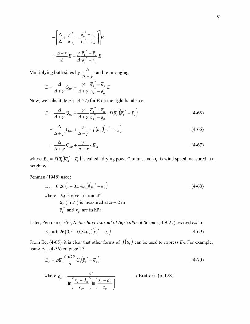
81

Eee

ee

as

aa

*

*

1

Eee

eeE

as

aa

*

*

Multiplying both sides by

and re-arranging,

Eee

eeQE

as

aane

*

*

Now, we substitute Eq. (4-57) for E on the right hand side:

asras

aane eeuf

ee

eeQE

*

*

*

(4-65)

aarne eeufQ

*

(4-66)

Ane EQ

(4-67)

where aarA eeufE * is called “drying power” of air, and ru is wind speed measured at a

height zr. Penman (1948) used:

aaA eeuE *254.0126.0 (4-68)

where EA is given in mm d-1

2u (m s-1) is measured at zr = 2 m

*

ae and ae are in hPa

Later, Penman (1956, Netherland Journal of Agricultural Science, 4:9-27) revised EA to:

aaA eeuE *254.05.026.0 (4-69)

From Eq. (4-65), it is clear that other forms of ruf can be used to express EA. For example, using Eq. (4-56) on page 77,

aaerA eeC

puE *622.0 (4-70)

where

0

0

0

0

2

lnlnz

dz

z

dzc

r

v

a

e

→ Brutsaert (p. 128)

82

When air travels over a large wet surface, it becomes vapor-saturated, i.e. ea ≅ ea

*. In such case, EA ≅ 0 in Eq. (4-67):

nee QE

(4-71)

Ee is referred to as “equilibrium” evaporation. The true equilibrium condition, however, rarely happens. → Brutsaert (p. 129) Priestley and Taylor (1972, Monthly Weather Review, 100: 81-92) reported an empirical relation:

neepe QE

(4-72)

where Epe is evaporation from wet surface e is a dimensionless coefficient

Since then, numerous studies have reported the applicability of Eq. (4-72) used with e = 1.2-1.3 to advection-free water surfaces and moist land surfaces. “Advection-free” means that the surface is large enough so that lateral transfer of energy from adjacent dry areas is negligible. Recall from Eq. (4-63):

ne

o

QB

E

1

1

Comparison of this with Eq. (4-72) shows that:

oe B

1

1

oe B

1

and 1

e

oB

(4-73)

Equation (4-72) has been used successfully with e = 1.26 over wet surfaces. This implies that Bo is relatively constant over wet surfaces for a given temperature.

→ Implication for climate warming? “Potential” evaporation is generally regarded as a fictitious quantity indicating the “maximum rate of evaporation from a large wet area”.

83

Despite the wide-spread use of this term, it is not clearly defined. Often, potential evaporation is determined using an evaporation pan placed on a dry land or a Penman-type equation (e.g. Eq. 4-65) that uses ea and Ta measured on dry land. However, dry land is clearly under a non-potential condition. → This contradicts the notion of “potential evaporation”. Therefore, the potential evaporation based on dry-land measurements should be called “apparent” potential evaporation, Epa, while “true” potential evaporation is denoted by Epo. → Brutsaert (p. 131) Many evaporation algorithms in hydrological models have a general form of:

E = eEp (4-74)

where e: empirical coefficient Ep potential evaporation e.g. Epa by Penman equation Epe by Eq. (4-72) Conceptually, e is dependent on soil moisture condition, crop growing stage, etc. A common approach is to assume:

c

cne ww

wwf

0

(4-75)

where fn( ) is an empirical function w is average water content of the “root zone” wc is cut-off water content (e.g. wilting point) w0 is maximum water content normally encountered in the root zone (field capacity) → Brutsaert (p. 131) An alternative approach to set e is offered by the resistance formulation (Brutsaert, pp. 133-135). In its simplest form, the resistance theory describes E as a flow of vapor through a series of two resistors. First: Resistance through stomata (rs) Second: Aerodynamic resistance (ra) Note that qs

* is the humidity of saturated air at Ts. In general, qs < qs

*, because the leaf surface is not completely wet. The stomatal resistance is defined by:

s

ss

r

qqE

* or

E

qqr ss

s

* (4-76)

84

Since E has units of kg m-2 s-1, the unit of rs is m-1 s, which is the reciprocal of velocity. In a similar manner, aerodynamic resistance is defined by:

a

as

r

qqE

or

E

qqr as

a

(4-77)

Recall from Eq. (4-54) that:

asre qquCE (4-78)

where

0

0

0

0

2

lnlnz

dz

z

dzC

r

v

a

e

Comparing Eq. (4-77) and (4-78),

rea uC

r1

(4-79)

Also, we can re-write the e-based Eq. (4-57) as:

asr qq

pufE

622.0 (4-80)

Substituting this into (4-77) gives: ra ufp

r622.0

Note that Eqs. (4-79) and (4-80) are generally applicable to any form of Ce or ruf .

Now, assume steady-state evaporation during the time scale of measurement (i.e. E = constant). From Eqs. (4-76) and (4-77),

Erqq sss * and Erqq aas

Errqqqq asasss *

as

as

rr

qqE

*

(4-81)

Equation (4-81) indicates that the “total” resistance for evaporation is given by rs + ra. → Analogous to a series circuit for electric current From Eqs. (4-8), (4-77), and (4-81)

a

sas

a

as

as

as

as

r

rrr

r

qq

qq

ee

ee

1

1** (4-82)

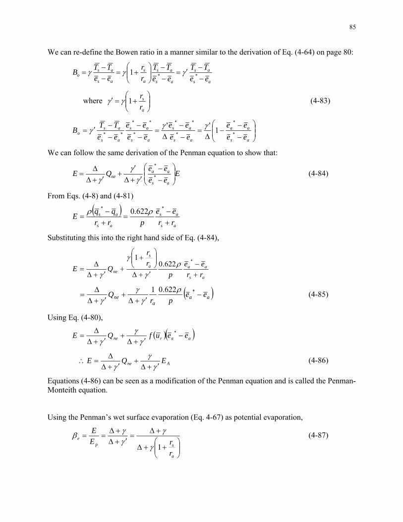
85

We can re-define the Bowen ratio in a manner similar to the derivation of Eq. (4-64) on page 80:

as

as

as

as

a

s

as

aso

ee

TT

ee

TT

r

r

ee

TTB

**1

where

a

s

r

r1

(4-83)

as

aa

as

as

as

as

as

aso

ee

ee

ee

ee

ee

ee

ee

TTB

*

*

*

**

*

**

**1

''

We can follow the same derivation of the Penman equation to show that:

Eee

eeQE

as

aane

*

*

(4-84)

From Eqs. (4-8) and (4-81)

as

as

as

as

rr

ee

prr

qqE

** 622.0

Substituting this into the right hand side of Eq. (4-84),

as

aaa

s

ne rr

ee

p

r

r

QE

*622.01

aa

ane ee

prQ

*622.01

(4-85)

Using Eq. (4-80),

aarne eeufQE

*

Ane EQE

(4-86)

Equations (4-86) can be seen as a modification of the Penman equation and is called the Penman-Monteith equation. Using the Penman’s wet surface evaporation (Eq. 4-67) as potential evaporation,

a

spe

r

rE

E

1

(4-87)

86

Equation (4-87) expresses the empirical “crop-coefficient” in terms of stomatal resistance. It appears to be more physically-based than Eq. (4-75), but in reality, we have merely replaced one empirical equation by another. → Brutsaert (p. 135) Numerous studies have tried to establish the relation between rs and plant growth stage, leaf area index, soil moisture, etc. Also, more sophisticated network of resistors is used to represent soil resistance, root resistance, etc. in the literature. Numerous other variants of the Penman method are found in the literature. For example, Granger and Gray (1989, Journal of Hydrology, 111: 21-29) defined a ratio G:

as

as

ee

eeG

*

(4-88)

Conceptually, G represents the ratio of non-wet surface to wet surface evaporation. Using Eq. (4-88) instead of (4-82), it can be shown that ( home work):

Ane E

G

GQ

G

GE

(4-89)

Granger and Gray (1989) attempted to express G as a “universal” function of the relative drying power D, defined by:

neA

A

QE

ED

(4-90)

For example, they proposed an empirical relation in the form of:

)045.8exp(028.01

1

DG

(4-91)

While this approach appeared to have been successful in their study sites, the “universal” function has not worked in other sites, such as Spy Hill Farm ( homework). 4.8 Eddy Covariance Method The application of eddy covariance method to E measurement is conceptually simple:

qwE (4-14b)

However, there are many practical issues to be considered for improving the accuracy. (1) Fetch requirement

87

Since the underlying theory (pages 67-68) is based on the homogeneous-boundary layer assumption, the instrument must be placed in a relatively large area with flat topography and uniform land cover. The instrumental “foot print” is generally considered to be roughly 100 times the height of instrument. → Schuepp et al. (1990, Boundary-Layer Meteorology, 50:355-373) (2) Orientation of the instrument The underlying theory requires 0w , but this may not be the case. If the orientation of the instrument is not perpendicular to the horizontal wind direction, the “tilt” correction is required. → Wilczak et al. (2001, Boundary-Layer Meteorology, 99:127-150) (3) Instrumental biases Several issues have been identified regarding the instruments used to measure wind, temperature, and humidity. → Oncley et al. (2007, Boundary-Layer Meteorology, 123:1-28) (4) Energy balance closure If E and H are accurately measured, from the energy balance requirement, we must have:

LeE + H = Qn ≅ Rn – G (4-92)

However, it has been commonly observed that:

(LeE + H)/ Qn ≅ 0.7-0.9

Despite the major research efforts by the flux measurement community, the cause of this consistently negative bias is not exactly known. It is believed that the large-scale eddies that are not captured by the instrument may be the most significant source of error. → See Oncley et al. (2007) For the time being, we need to choose between: (a) Use the raw LeE data for hydrological studies, admitting that it probably underestimates

actual evaporation flux. → Undesirable for water balance studies. See Barr et al. (2012, Agricultural and Forest Meteorology, 153:3-13). (b) “Correct” LeE and H data so that Eq. (4-92) is satisfied. → Twine et al. (2000, Agricultural and Forest Meteorology, 103:279-300) If we choose (b), two approaches are available: - Assume that H is correctly measured. i.e. LeE = Rn – G – H (4-93)

- Assume that LeE and H are biased by the same relative amount. i.e. Bo = H/LeE is correctly measured.

measurede

en

oncorrecte ELH

ELGR

BGREL

)(1

1)(

(4-94)