4 DIFFERENTIAL KINEMATICS

Purpose:

The purpose of this chapter is to introduce you to robot motion. Differential forms of the homogeneous transformation can be used to examine the pose velocities of frames. This method will be compared to a conventional dynamics vector approach.

The Jacobian is used to map motion between joint and Cartesian space, an essential operation when curvilinear robot motion is required in applications such as welding or assembly.

4.1 Differential Displacements

Often it is necessary to determine the effect of small displacements on kinematic trans-formations. This can be useful in trajectory planning and path interpolation/extrapolation or in interacting with sensor systems such as vision or tactile. Now if we have a frame T relating a set of axes (primed axes) to global or base axes, then a small differential dis-placement of these axes (dp, d = dk) relative to the base axes results in a new frame T' = T + dT = H(ddp) T. Although finite rotations can't be considered vectors, differ-ential (infinitesimal) rotations can, thus d = d k. Thus, the form of dT can be ex-pressed as

dT = (H(ddp) - I) T = T (4.1)

Equation (4.1) expresses the differential displacement in base coordinates. Displace-ments made relative to the primed axes ( dp, dexpressed in primed axes)change the form of dT to

dT = T (H(ddp) - I) = T T (4.2)

Considering translation and rotation separately, and defining or T (depending upon the axes of reference) equal to H(ddp) - I, we determine that

H (d) = R (d) 00T 1

where

R (d) = 1 -kzd kyd

kzd 1 -kxd-kyd kxd 1 (4.3)

Equation (4.3) comes from (2.1) using sin d d, and cos d 1.

4-1

For pure differential translation,

H (dp) = I dp

0T 1 (4.4)where

dpT = dpx dpy dpz

Now since H(d, dp) = H (dp) H(dit is easily shown that,

(d, dp) = H(dp) H(d) - I

(4.5)

Given (4.5), d and dp, dT can be determined in either (4.1) or (4.2) and the natural ex-tension to velocities of points within these frames appropriately follows.

In the case of pure rotation, (4.5) reduces to a differential screw rotation about the unit vector k since the differential translation in the 4th column reduces to zero. Taking the de-rivative of (4.5) we generate the screw angular velocity matrix of equation (4.7) in Tsai's text:

(4.6)

4.2 Relating Differential Transformations to Different Coordinate Frames

Given dT relative to the base axes, what is the differential transformation in x'y'z' such that T = T T? In other words, given dT how are and Trelated? The relation-ship is defined by equating (4.1) and (4.2) so that

T = T T

which can be solved for = T TT-1 (4.7)

or

4-2

T= T-1 T (4.8)

To determine the components of (4.7) and (4.8), let

T =

ax bx cx pxay by cy pyaz bz cz pz

0 0 0 1

and define the differential rotations and translations relative to base axes by

= x i + yj + zkd =dxi + dyj + dzk

where

x = dx dx = dpx

y = dy dy = dpy

z = dz dz = dpz

Thus,

=

0 -z y dx

z 0 -x dy

-y x 0 dz0 0 0 0 (4.9)

which comes from (4.5) by noting that x = kx d, y = ky d, and z = kz d (the direc-tion cosines resolve d into its i, j, and k components).

Pre-multiplying T by it can be shown that T assumes the form

T =

x a x x b x x c x x p + d x

x a y x b y x c y x p + d y

x a z x b z x c z x p + d z 0 0 0 0 (4.10)

Premultiplying by T-1 to obtain (4.8),

T = T-1 T =

a · ( x a) a · ( x b) a · ( x c) a · ( x p ) + db · ( x a) b · ( x b) b · ( x c) b · ( x p) + dc · ( x a) c · ( x b) c · ( x c) c · ( x p) + d

0 0 0 0 (4.11)

Equation (4.11) can be reduced using

4-3

a · (b x c) = -b · (a x c) = b · (c x a)a · (b x a) = 0 a x b = cb x c = ac x a = b

to the form,

T =

0 - · c · b · (p x a) + d x a · c 0 - · a · (p x b) + d x b- · b · a 0 · (p x c) + d x c 0 0 0 0 (4.12)

But in terms of differential displacements relative to the primed axes

T =

0 -z' y' dx'

z' 0 -x' dy'

-y' x' 0 dz' 0 0 0 0 (4.13)

Equating (4.12) and (4.13),

x' = · a = T a (4.14a)y' = · b = T b (4.14b)z' = · c = T c (4.14c)

dx' = · (p x a) + d · a (4.15a)dy' = · (p x b) + d · b (4.15b)dz' = · (p x c) + d · c (4.15c)

Note that we can easily determine the elements of given the elements of T by apply-ing the relationship = T TT-1 which can be gathered into the form of (4.7) as,

= (T-1)-1 TT-1 (4.16)

Thus we can apply (4.14) and (4.15) by simply using T and the inverse of T.

4.3 Velocities

Vector w can be resolved into components p in the base frame by the equation p = T w. Now under a small rotation/displacement, frame T can be expressed by the new frame

T' = T + dT = T + ∆T (4.17)

A vector w in frame T, once perturbed, can be located globally by p' such that p' = (T + T) w (4.18)

4-4

The delta move, p' - p, becomes

p' - p = (T + T) w - T w = T w

Figure 4-1 Velocity of a point in a moving frame

Dividing by t and taking the limit as t 0 (take derivative), we determine the velocity in the base frame:

(4.19)

where

(4.20)

which can be reduced to the simpler form

(4.21)

expressed in angular and curvilinear velocity components.

4.3.1 Example

A point P is located by vector in frame C as shown in Figure 4-2. At this instant the frame C origin is being translated by the velocity vt = 2 I + 2J m/s relative to the base

4-5

frame. The frame is also being rotated relative to the base frame by the angular velocity = 2 rad/s K where I J K are the unit axis vectors for the base frame. Determine the in-stantaneous velocity of point P using both the conventional vector dynamics approach and also using the differential methods in this chapter.

Conventional:

v = vo + x

where vo = vt + x r. At this instant note that frame C is aligned with the base frame so that the unit axes vectors are parallel.

It can be shown that x r = -6I + 4J so that

vo == 2 I + 2 J -6 I + 4 J = -4 I + 6J m/s

It can be shown that x = -10 I + 6 J, so that

v = -4 I + 6J -10 I + 6 J = -14 I + 12 J m/s

Differential transformations:

Apply

where w = and

4-6

xr

Y

y

X

P (3,5,0) relativeto frame C

Frame C

2 rad/s

(2,3,0)

p

Figure 4-2 Example

O

to give

Note that the same values are obtained!

4.4 Jacobians for Serial Robots

The Jacobian is a mapping of differential changes in one space to another space. Obvi-ously, this is useful in robotics because we are interested in the relationship between Cartesian velocities and the robot joint rates.

If we have a set of functions

yi = fi(xj) i = 1,...m; j = 1,...n (4.22)

then the differentials of yi can be written as

i = 1, . . .m (4.23)

or in matrix form,

y = J x (4.24)where

J = Jacobian = (4.25)

In the field of robotics, we determine the Jacobian which relates the TCF velocity (posi-tion and orientation) to the joint speeds:

(4.26)

(4.27)

4-7

where

v is the TCF origin velocity is the orientation angular velocity (equivalent Euler angles, etc.)

q is the joint velocities (joint rotational or translation speeds)

Waldron in the paper "A Study of the Jacobian Matrix of Serial Manipulators", June, 1985, ASME Journal of Mechanisms, Transmissions, and Automation in Design, deter-mines simple recursive forms of the Jacobian, given points on the joint axes (ri) and joint direction vectors (ei) for the joint axes. The velocity of point P, a point on some end-ef-fector, can be determined by the following equation, reference Figure 4-3:

P

Joint 1

Joint i+1

Joint n

Joint i

rr

r

r

n

1 ii+1

i

e

e

e

e

n

i+1

1

i

Figure 4-3 Waldron's notation

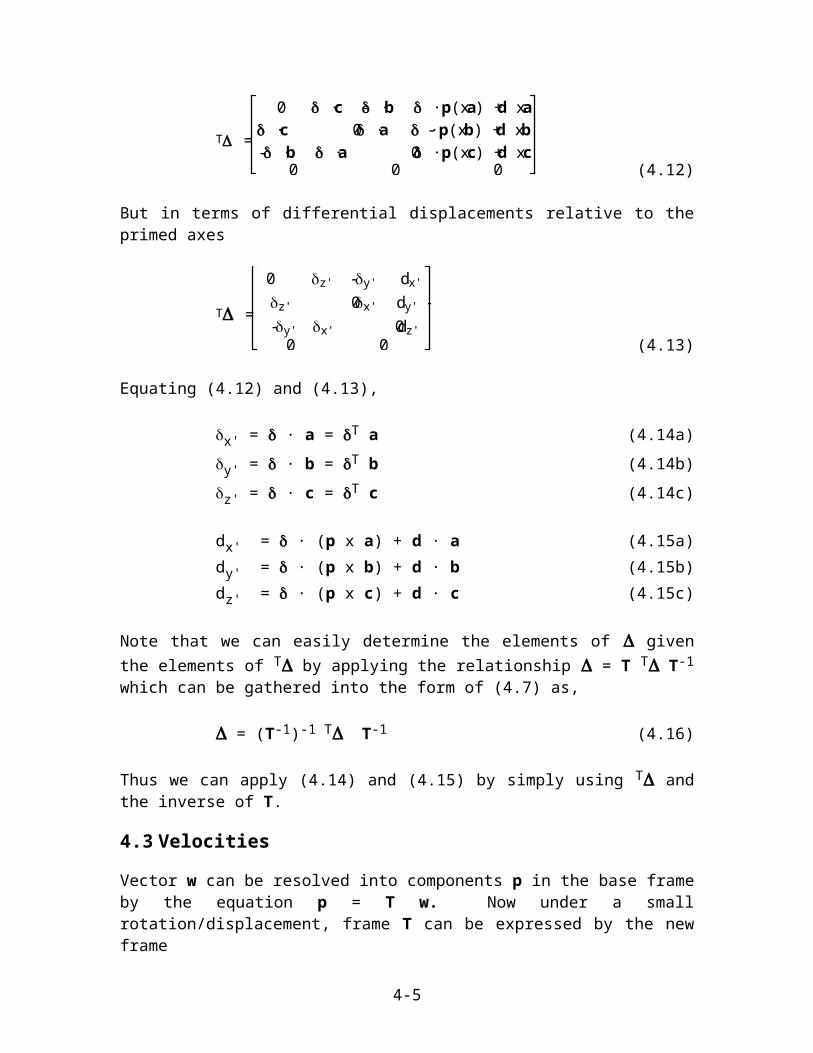
(4.28)

Equation (4.28) can also be reduced to the form

(4.29)

where i is the absolute angular velocity of link i and i is the position vector between joint axes i+1 and i:

(4.30)

4-8

The Jacobian is determined by collecting the velocities for each joint into the form:

(4.31)

and the velocity relationship becomes:

"R" "P"

(4.32)

Given the TCF velocity, we determine the joint velocities by the inverse Jaco-bian:

q = J-1 V (4.33)

Waldron, et. al., illustrate several closed form solutions for the Jacobian, but, in general, there is no general closed form solution for robots with arbitrary structures. Note that J-1

only exists for a six-axis robot. Robots with less than 6 joints map the joint space into a subspace of Cartesian space. For example, a cylindrical robot will typically map the one or two rotational joints into one angular velocity component (usually about the base frame Z-axis).

Six-axis robots often will display configurations where joints line up. We refer to this as joint redundancy. In these cases J-1 is undefined because the rank of J is less than 6 and the J determinant vanishes. There are also singular configurations where det(J) = 0 be-cause motion in Cartesian space causes large joint rates - see Figure 4-4.

4.5 Serial Robot Singularities

Consider a serial mechanism and its Jacobian J that maps the joint motion to the end-ef-fector (tool) motion:

v = J (4.34)

Vector v is a mx1 vector of tool velocity components in Cartesian space (sometimes re-ferred to as task space), while is a nx1 vector of the mechanism joint rates for n joints. Normally m = 6. The space of the tool motion is sometimes referred to as the operational space.

For convenience we assume that the robot’s tool origin coincides with the origin of the terminal joint. In the case where the mechanism has a 3 joint terminal sequence arranged as a spherical joint, we choose the concurrent point of the last 3 joints. This choice will simplify the investigation of motion singularities.

4-9

Figure 4-4 Singularity for serial robot

Assuming full (R6) Cartesian mobility, the Cartesian ve-locity components in v cor-respond to 3 orthogonal an-gular components and 3 or-thogonal linear components (shown in row form):

vT = [ x y

z vx vy vz] (4.35)

The Jacobian may be re-solved into the robot’s base frame or into any selected joint frame. If a robot has a terminal spherical joint se-quence, as is the case with many robots, and depending on the robot type, it may be useful to resolve the Jaco-bian into joint 4 to decouple the orientation and linear components.

Mechanisms that have < 6 joints should have their zero (or dependent) rows removed from the Jacobian, also removing the corresponding Cartesian velocity components from v (leaving m = 6 or less components) These components correspond to Cartesian task motion components that cannot be generated by any mechanism joint motion. For exam-ple, a mechanism that has only one revolute axis will only be able to generate one of the Cartesian angular velocity components in (4.35).

If Cartesian motion is specified, then robot control must determine the appropriate joint rates from

= J-1 v (4.36)

This requires that J be square and invertible. We can determine invertibility by the deter-minant of J, namely |J|. The Jacobian’s rank depends on the mechanism’s kinematics configuration, number of joints, and joint types. Motion at a singularity will reduce the rank, resulting in |J| = 0. Motion near a singularity will cause |J| to approach zero and generally lead to higher joint velocities near singularities. At or near a singularity the ro-bot’s tool will either lose some directional Cartesian mobility (even though robot joints can move), or require some joints to move at high speeds to attain the mobility.The robot is degenerate in configurations that cause it to lose mobility in certain direc-tions. These directions are referred to as degenerate directions that cannot be instanta-neously achieved with any joint motion. Effectively, robot mobility is limited at or near the current configuration.

4-10

c) Spherical joints origin loses position mobility by lying on first joint axis.

Figure 4-5 – Typical singularities

b) Singularity due to joints 4 and 6 alignment

a) Boundary singularity

4.5.1 Singularity Types

Three singularities are shown in Figure 4-5. Fig. 4-5a, the workspace boundary singular-ity, occurs when joint 3 is zero (or 180 degrees) and links 2 and 3 are radially extended (or folded). The line along extended (or folded) links 2 and 3 is called a degenerate di-rection because it is not possible to move the robot’s tool point in this direction without very large joint 2 and 3 motions.

In Fig. 4-5b joints 4 and 6 of the spherical joint sequence are co-linear when joint 5 is zero. Thus, joints 4 and 6 are redundant with respect to their aligned rotational axes. This singularity is called a redundancy singularity. Others call it a self-motion singularity be-cause joints 4 and 6 can be rotated in a correlated fashion so that the tool does not rotate about the direction co-linear with joint axis 4 and joint axis 6. In fact the tool will not move or rotate in Cartesian space if joints 4 and 6 are rotated oppositely. In such cases we set v = 0 and reduce (4.34) to the form:

J = 0 (4.37)

Equation (4.37) expresses configurations where J has a null space. The trivial solution represented by = 0 exists when J is not singular. When J is singular and thus |J| = 0, there are solutions where is not zero and (4) is satisfied. This defines mathematically a self-motion singularity. Mechanisms with self-motion singularities will exhibit (4.37) at selected configurations. Some methods for moving through self-motion singularities will reconfigure the mechanism using the relation (4.37) since the tool is not moved, and then escape the singularity using this new configuration. This means that the mechanism is slowed, then stopped, at the singularity, reconfigured, and then a new path planned to es-cape the singularity. This may not be feasible in many tasks.

Note in Figure 4-6 that if the task motion requires that the tool be rotated about a screw axis instantaneously perpendicular to the plane containing joint axes 4 and 5, without changing the position of the tool point, it is not possible without an infinite joint 5 rate. This perpendicular axis is the degenerate direction.

In Fig. 4-5c the spherical joint origin (concurrent intersection point of last 3 joints) lies on the vertical joint axis of joint 1. Thus, joint one motion cannot change the spherical joint origin position and the robot loses design mobility. In fact, there is no motion of the first 3 joints that can instantly move the tool point perpendicular to the plane of links 2 and 3 when links 2 and 3 are not co-linear. This is a degenerate direction - another exam-ple of a self-motion singularity - which is removed if the tool point does not lie on the first joint axis. It is possible to move the spherical joints in such a way as to cancel out the joint 1 rotation of the tool, keeping the tool point fixed in space. Thus, the null space equation (4.37) holds for this singularity.

4-11

More than one singularity can occur at the same time. For this robot, if the ro-bot is extended radially and vertically up and joint 5 is also zero, then the rank of the Jacobian, normally 6, will be reduced to 3.

The self motion singularities just de-scribed may have an infinite number of non-feasible directions, since there are an infinite number of unique task space directions that give a non-zero projection onto the degenerate direc-tion. For example, consider the Fig. 4-5b singularity shown in Figure 4-6. The degenerate direction is perpendic-ular to the plane of the z4/z6 and z5

joint axes. The robot cannot instantly rotate about this axis and keep the robot tool posi-tion fixed. In fact, any task space rotational axis that does not lie in the plane of z 4/z6 and z5 is not feasible until axis 5 is first rotated – see the dashed screw axis in Figure 4-6.

4.5.2 Motion Planning Near or Through Singularities

It would seem that there are two cases that must be considered when moving near or through singularities, when the task cannot avoid the singularities:

Case 1 - moving through a singularityCase 2 - moving near a singularity, but not through a singularity

Case 1 should be avoided, but this may not always be possible, depending on the task re-quirements and the mechanism type. Mechanisms like robots have different types of sin-gularities and related degenerate directions. Some singular configurations can be tra-versed with proper motion planning, while others cannot without an additional sequence of internal joint motions that may not maintain the desired tool motion. For example if the robot of Fig. 4-5 is moved in joint space to a configuration where joint 5 is zero, then it is not possible to rotate the tool around the degenerate direction in Figure 4-6 without infinite joint 5 rates.

Now consider that the robot’s tool in Figure 4-5a (boundary singularity) is to be moved radially inward at a specified velocity. This is not feasible without impossibly large joint 2 and 3 rates, yet possible if the tool velocity can be relaxed locally by having the joint 2 and 3 rates slowly increase. The tool velocity can be planned to slowly increase until the desired value can be achieved as the robot moves away from the singular configuration. Reference [1] describes this type of trajectory motion near this type of singularity, but does not offer any methods new to the DMAC lookahead methods.

In general, Case 2 motion near singularities will cause excessive joint rates, requiring the Cartesian motion be slowed accordingly. Cartesian slowing may not always be feasible,

4-12

z5 z4, z6

Degenerate direction

Fig. 4-6 – Degenerate direction

z5

depending on the task (e.g., welding, painting). Motion at or near a singularity must con-sider the degenerate directions and the type of singularity. Motion along/about a degener-ate direction is not possible without one or more joints experiencing excessive rates. In fact any motion that has a projection component on the degenerate direction may not be feasible because of large joint rates. In these situations the Cartesian motion must either be slowed significantly to move through or about the singularity or the Cartesian motion be converted to joint motion. In applications that demand close path following, where only slight path deviations are allowed, there is no alternative.

One method often referenced is the damped least squares method [2], [3] which damps/slows the task motion in proximity to singular configurations. Reference [4] describes a related method, called natural motion, which also slows motion in proximity to singular configurations but with some loss of path accuracy. Researchers are quick to note that the resulting path may not approximate true paths well and, in the case of references [2] and [3], the end-effector path may not reach or pass through the singularity, if required. Al-though these methods may be viable for tasks like part assembly that do not require true path following, they fail when path following must be accurate.

Observation - DMAC is presently designed with lookahead methods to determine joint values along the path, for identifying cases where large joint changes occur over small path displace-ments, signaling singularity or nearness to singularity. When such cases occur, the Cartesian path motion can be slowed to bring the joint rates (including joint accelerations) to within limits or, al -ternatively, the motion can be transitioned to joint space when near singularities. Shifting the mo-tion to joint space will require a finer spacing of trajectory points along the path to maintain path accuracy. A question to be answered is how much the joint space trajectory deviates from the true path when using a joint space transition scheme.

Nearness of singularity can be measured by the value of |J| as it approaches zero to within some tolerance. In cases where the mechanism exhibits more than one singularity the Jacobian determinant can be expanded into the form [4.38]:

|J| = s(q) = s1(q) s2(q)…sk(q) (k = number of singularities), (4.38)

where one or more of the singularity functions si(q) will vanish at a singularity configu-ration. Given (4.38) it is not clear how to determine nearness to singularity configuration, since a number of functions si(q) are involved. One could assign nearness by the condi-tion:

if |si(q)| < i for any i = 1, 2,…, k configuration near singularity(s) (4.39)

by setting appropriate values for the tolerances i. Unfortunately, what defines proper tol-erances is not clear.

Alternatively, we could use the Jacobian determinant in the following check:

if |J| < , motion near singularity(s) (4.40)

where we must again determine an appropriate . The advantage of (4.39) is that it will identify the singularity type.

4-13

Reference [6] is an example by one of a number of researchers that considers how to move around singularities. The approach is to remove the degenerate direction(s) from the Jacobian by removing the appropriate row(s) at or near the singularity. Motion plan-ning is then conducted in the space orthogonal to the degenerate direction(s), since the reduced Jacobian only allows this type of motion. This also constrains the possible path directions which may not be feasible if the actual path has motion components along the degenerate direction. In these cases a conversion to joint motion may be necessary to make the transition. We will name the conversion to joint motion the Joint Transitional Method (JTM) and consider it in a separate section.

Another approach often used to identify nearness to singular configurations is Singular Value Decomposition (SVD) on J, which will generate and sort in descending order the diagonal terms in the diagonal matrix that get smaller as the mechanism motion ap-proaches singularities. If the mechanism is far removed from any singularity configura-tions no diagonal terms will be small.

The decomposition form is

J = U VT, (4.41)

where U and VT are basis matrices for Cartesian space and joint space, respectively, with their columns serving as orthonormal basis vectors for their two respective spaces. Refer-ence [4] notes that, at singular configurations, the last columns of U, with number equal to the rank deficiency of the Jacobian, represent basis vectors for the singular subspace. Any vector in this subspace is degenerate, and any path whose projection onto this sub-space is non-zero will likewise be degenerate. Any paths that lie in the subspace orthogo-nal to the singular subspace (expressed by the subspace of the first columns of U) will not be degenerate and will not experience large joint rates. Thus, SVD methods can es-tablish feasible path directions near singular points that do not cause large joint values. If you have the freedom to deviate the path, then these methods may be useful. A limitation is that calculating the SVD of J can be computationally expensive.

4.5.3 Conclusions

Researchers have examined motion around singularities using a number of methods, many not mentioned here. But a fundamental premise of these methods is that path devi-ations are allowed around singularities (in some cases a sharp reduction in path velocities may be also allowed). A question not answered in these papers is how much deviation is allowed and how to select paths when several path choices are available. Unfortunately, many real tasks do not permit these deviations.

A few of the papers have mentioned conversion to joint motion as a solution, but without further detail. This simpler transitional approach is probably the preferred approach used by many vendors.

4.6 Differential Motion Summary for Serial Robots

4-14

Differential forms can be applied to generate motion of frames or of points in frames when the frame experiences translational and/or angular motion. This method can be simpler to apply than the conventional vector equations.

The Jacobian is important in robotics because the robot is controlled in joint space, whereas the robot tool is applied in physical Cartesian space. Unfortunately, motion in Cartesian space must be mapped to motion in joint space through an inverse Jacobian re-lation. This relation might be difficult to obtain.

The equations for the Jacobian are easy to determine for a robot, given the current robot configuration, as outlined by Waldron et. al in the paper "A Study of the Jacobian Matrix of Serial Manipulators", June, 1985, ASME Journal of Mechanisms, Transmissions, and Automation in Design.

4.7 Jacobian for Parallel Robots

Let us define two vectors: x is a vector that locates the moving platform, while q is a vector of the n actuator joint values. In general the number of actuated joints is equal to the degrees-of-freedom of the robot.

The kinematic constraints imposed by the limbs will lead to a series of n constraint equa-tions:

f(x,q) = 0 (4.42)

We can differentiate (4.42) with respect to time to generate a relationship between joint rates and moving table velocities:

Jx = Jq (4.43)

where Jx = f/x and Jq = - f/q.

Thus, the Jacobian equation can be written in the form

= J (4.44)

where J = Jq-1 Jx.

Note that equation (4.44) is already in the desired inverse form, given that we can deter-mine Jq

-1 and Jx.

4.7.1 Singularity Conditions

A parallel manipulator is singular when either Jq or Jq or both are singular. If det(Jq) = 0, we refer to the singularity as an inverse kinematics singularity. This is the kind of singu-larity where motion of the actuation joints causes no motion of the platform along certain directions. For the picker robot this occurs when the limb links all lie in a plane (2i = 3i

4-15

= 0). This case is similar to the case shown in Figure 4-4 for a serial robot.

If det(Jx) = 0, we refer to the singularity as a direct kinematics singularity. This case occurs for the picker robot when all upper arm linkages are in the plane of the moving platform - see Figure 4-7. Note that the actuators cannot resist any force applied to the moving platform in the z direction.

4.8 Jacobian for the Picker Ro-bot

Referring back to equation (3.30) in the notes, we can write the loop equation

OP + PCi = OAi + AiBi + BiC (4.45)to close the vector from the base frame to the center of the moving platform. We differ -entiate (4.45) to obtain the equation

vp = 1i x ai + 2i x bi (4.46)

for the velocity of the moving platform at point P and where ai = AiBi and bi = BiCi.

The last term in (4.46) is a function of the passive joints. We can eliminate them from the equation by dot multiplying (4.46) by bi to get

bi vp = 1i (ai x bi) (4.47)

Expressing these vectors in the ith limb frame, we can get

jix vpx + jiy vpy + jiz vpz = a s2i s3i (4.48)

where

jix = c(1i + 2i) s3i ci - c3i si (4.49a)

jiy = c(1i + 2i) s3i si + c3i ci (4.49b)

jiz = s(1i + 2i) s3i (4.49c)

We can assemble (4.48) and (4.49) into equations for each limb by the matrix equation:

Jx vp = Jq (4.50)

4-16

Figure 4-7

where

Jx = (4.51)

Jq = a (4.52)

Question: What observation can you make from the forms of (4.50) - (4.52)?

4.9 Jacobian Summary

The Jacobian in robotics is particularly important because it represents the rate mapping between joint and Cartesian space. Unfortunately, for serial robots the desire is to deter-mine the joint rates to get desired motion in Cartesian space as the tool is moved along some line in space. This usually requires the inverse of the Jacobian, which may be diffi-cult for some mechanisms.

The Jacobian for parallel robots may be easier to find, as is the case for the Picker robot.

4.10 References

1. Lloyd, J.E., and Hayward, V., “Singularity-Robust Trajectory Generation,” Intl J. of Robotics Research, Vol. 20, No. 1, pp 38-56, 2001.

2. Nakamura, Y., and Hanafusa, H. 1986. Inverse kinematics solutions with singu-larity robustness for robot manipulator control,” Trans. ASME, J. Dynamic Sys-tems, Measurement and Control 108:163–171.

3. C.W. Wampler 11, “Manipulator inverse kinematics solutions based on vector formulations and damped least-squares meth-ods,” IEEE Trans. on Systems, Man and Cyb., Vol. SMC-16, No. 1, pp. 93-101, 1986.

4. D. N. Nenchev, Y.Tsumaki, and M. Uchiyama, “Singularity-Consistent Parameterization of Robot Motion and Control,” Intl J. of Robotics Research, Vol. 19, No. 2, pp 159-182, 2000.

5. K-S. Chang, and O. Khatib, “Manipulator Control at Kinematics Singularities: A Dynamically Consistent Strategy,” Proc. IEEE/RSJ Int. Conference on Intelligent Robots and Systems, Pittsburgh, August 1995, vol. 3, pp. 84-88.

6. D. Oetomo, M. H. Ang, and S. Y. Lim, “Singularity handling on PUMA in opera-tional space formulation,” in Lecture Notes in Control and Information Sciences,

4-17

Eds. Daniela Rus and Sanjiv Singh, Eds., vol. 271, pp. 491–501. Springer – Ver-lag, 2001.

4-18