4. Continuous Symmetries

So far we have focussed almost exclusively on the Ising model. Now it is time to

diversify. First, however, there is one more lesson to wring from Landau’s approach to

phase transitions. . .

4.1 The Importance of Symmetry

Phases of matter are characterised by symmetry. More precisely, phases of matter are

characterised by two symmetry groups. The first, which we will call G, is the symmetry

enjoyed by the free energy of the system. The second, which we call H, is the symmetry

of the ground state.

This structure can be seen in the Ising model. When B = 0, the free energy has

a G = Z2

symmetry. In the high temperature, disordered phase this symmetry is

unbroken; here H = Z2

also. In contrast, in the low temperature ordered phase, the

symmetry is spontaneously broken as the system must choose one of two ground states;

here H = ?. The two di↵erent phases – ordered and disordered – are characterised by

di↵erent choices for H.

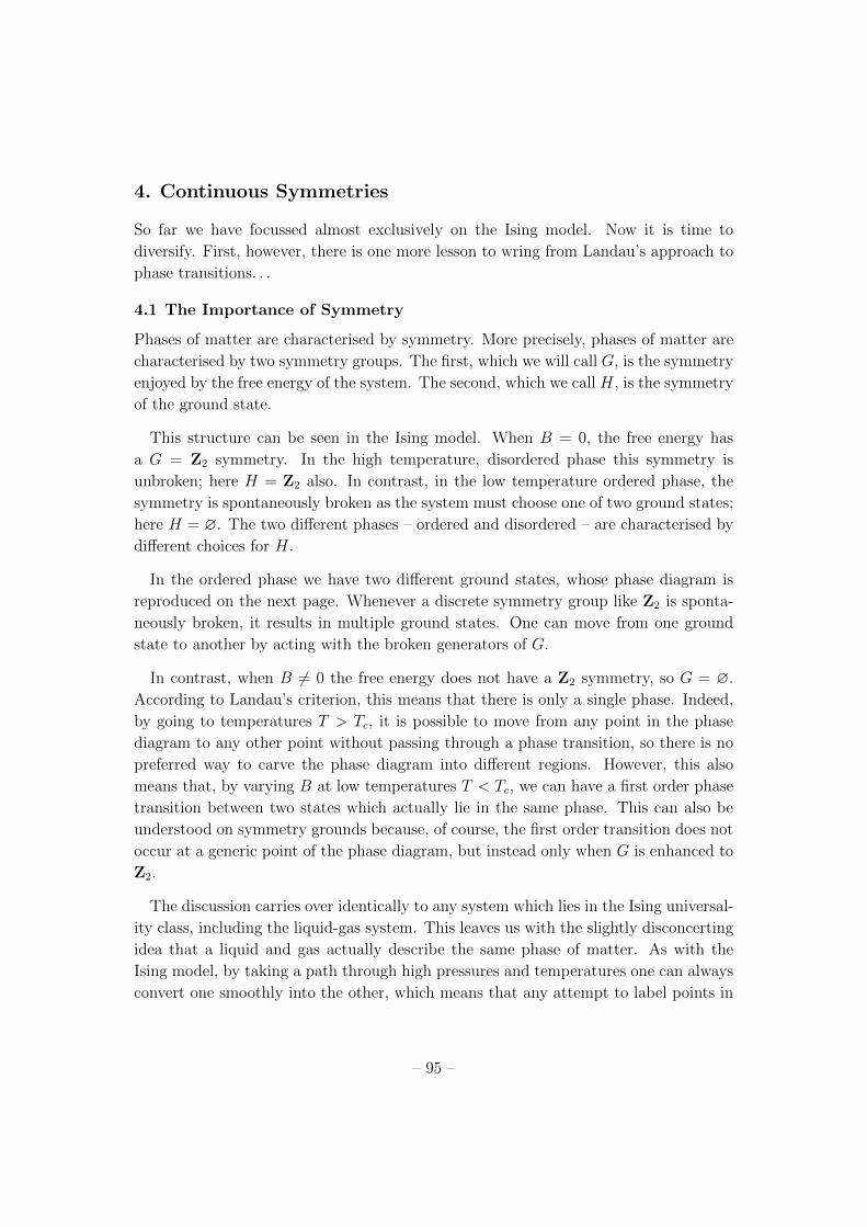
In the ordered phase we have two di↵erent ground states, whose phase diagram is

reproduced on the next page. Whenever a discrete symmetry group like Z2

is sponta-

neously broken, it results in multiple ground states. One can move from one ground

state to another by acting with the broken generators of G.

In contrast, when B 6= 0 the free energy does not have a Z2

symmetry, so G = ?.

According to Landau’s criterion, this means that there is only a single phase. Indeed,

by going to temperatures T > Tc

, it is possible to move from any point in the phase

diagram to any other point without passing through a phase transition, so there is no

preferred way to carve the phase diagram into di↵erent regions. However, this also

means that, by varying B at low temperatures T < Tc

, we can have a first order phase

transition between two states which actually lie in the same phase. This can also be

understood on symmetry grounds because, of course, the first order transition does not

occur at a generic point of the phase diagram, but instead only when G is enhanced to

Z2

.

The discussion carries over identically to any system which lies in the Ising universal-

ity class, including the liquid-gas system. This leaves us with the slightly disconcerting

idea that a liquid and gas actually describe the same phase of matter. As with the

Ising model, by taking a path through high pressures and temperatures one can always

convert one smoothly into the other, which means that any attempt to label points in

– 95 –

B

T

TC

Tc

p

T

gas

liquid

Figure 31: The phase diagram of the

Ising model (again).

Figure 32: The phase diagram of the

liquid-gas system (again).

the phase diagram as “liquid” or “gas” will necessarily involve a degree of arbitrariness.

It is really only possible to unambiguously distinguish a liquid from a gas when we sit

on the line of first order phase transitions. Here there is an emergent G = Z2

symme-

try, which is spontaneously broken to H = ?, and the two states of matter – liquid

and gas – are two di↵erent ground states of the system. In everyday life, we sit much

closer to the line of first order transitions than to the critical point, so feel comfortable

extending this definition of “liquid” and “gas” into other regimes of the phase diagram,

as shown in the figure.

Beyond Ising

The idea of symmetry, and of broken symmetry, turns out to be useful in characterising

nearly all phases of matter. In each case, one should first determine an order parameter

and a symmetry group G under which it transforms. Sometimes the choice of order

parameter is obvious; sometimes it is more subtle. One then writes down the most

general Landau-Ginzburg free energy, subject to the requirement that it is invariant

under G. The di↵erent phases of matter within this class are characterised by the group

H preserved by the ground state.

There are a number of reasons why it is useful to characterise states of matter in

terms of their (broken) symmetry. The original idea of Landau was that, as we’ve

seen with the Ising model, symmetry provides a powerful mechanism to understand

when a phase transition will take place. In particular, there must be a phase transition

whenever H changes.

However, it turns out that this is not the only thing symmetry is good for. As we

will see below, knowledge of G and H is often su�cient to determine many of the low

energy properties of a system, both through a result known as Goldstone’s theorem

– 96 –

(that we will describe in Section 4.2) and through various topological considerations

(some of which we will see in Section 4.4).

Finally, and particularly pertinent for this course is the role that symmetry plays in

the renormalisation group and specifically in universality. One can ask: when do two

systems lie in the same universality class? Although the full answer to this question is

not yet understood, a fairly good guess is: when they share the same symmetry G.

There are many di↵erent systems and choices of G that we could look at. A par-

ticularly interesting class occurs when we take G = Rd ⇥ SO(d), the group of spatial

translations and rotations. The pattern of symmetry breaking provides, for example, a

clean distinction between a liquid/gas and a solid, with the latter breaking G down to

its crystal group. In this framework, there is not one solid phase of matter, but many,

with each di↵erent crystal structure preserving a di↵erent H and hence representing

a di↵erent phase of matter. The di↵erent breaking patterns of spatial rotations also

allows us to define novel phases of matter, such as liquid crystals. Viewed in this way,

even soap, which can undergo a discontinuous change to become slippery, constitutes

a new phase of matter. We will not discuss this form of symmetry breaking in this

course, but you can learn more about it in next term’s course on Soft Matter.

Here, instead, we will be interested in phases of matter that are characterised by

“internal” symmetry groupsG that are continuous, as opposed to the discrete symmetry

of the Ising model. This includes materials like magnets, where the spin is a vector

that is free to rotate. It also includes more exotic quantum materials such as Bose-

Einstein condensates, superfluids and superconductors. We will see that systems with

continuous symmetry groups G exhibit a somewhat richer physics than we’ve seen in

the Ising model.

Beyond the Landau Classification

The idea that phases of matter can be classified by (broken) symmetries has proven

crucial in placing some order on the world around us. However, it is not the last

word. Over the past twenty years, it has become increasingly clear that certain highly

entangled quantum systems defy a simple characterisation by symmetry. The first,

and most prominent, examples are the quantum Hall states. To understand these, one

needs a new ingredient: topology. We will not touch upon this here, but you can read

more in the lecture notes on the Quantum Hall E↵ect.

– 97 –

4.2 O(N) Models

Phases of matter that are characterised by continuous, as opposed to discrete, symme-

tries o↵er a rich array of new physics. The simplest such models contain N real scalar

fields, which we arrange in a vector

�(x) = (�1

(x),�2

(x), . . . ,�N

(x))

We will ask that the free energy is invariant under the O(N) symmetry

�a

(x) ! R b

a

�b

(x)

where R 2 O(N) so that RTR = 1. Now, when constructing the free energy we write

down only the terms invariant under O(N). The first few are

F [�(x)] =

Z

ddx

�

2r� ·r�+

µ2

2� · �+ g(� · �)2 + . . .

�

where rotational invariance requires r� · r� = @i

�a

@i

�a

. These kind of theories are

known, not unreasonably, as O(N) models. They are of interest for all N , but N = 2

and N = 3 play particularly prominent roles.

O(2): The XY-Model

When N = 2, it is often convenient to pair the two real scalar fields into a single

complex field

(x) = �1

(x) + i�2

(x)

The free energy now consists of all terms which are invariant under U(1) phase rotations,

! ei↵ . The first few terms are

F [ (x)] =

Z

ddr

�

2r ? ·r +

µ2

2| |2 + g| |4 + . . .

�

(4.1)

This is also known as the XY-model or, sometimes, the rotor model.

There are at least two physical systems which sit in this universality class. The first

are magnets where, in contrast to the Ising model, each atom has a continuous spin s

which can rotate in a plane. (This is usually taken to be the X � Y plane, which is

where the name comes from.) The microscopic Hamiltonian is the generalisation of the

Ising model (1.1) to

E = �JX

hijisi

· sj

(4.2)

– 98 –

where |si

| = 1. This is also written as

E = �JX

hijicos(✓

i

� ✓j

)

where ✓i

is the angle that the spin si

makes with some, fixed reference direction. Coarse-

graining this microscopic model gives rise to the free energy (4.1). One could also add

a magnetic field termP

i

B · si

, where B is also a two-component vector. Such a term

would break the O(2) symmetry, and introduce terms in (4.1) that are odd in .

The second physical system described by (4.1) is rather di↵erent in nature: it is a

Bose-Einstein condensate, or its strongly coupled counterpart, a superfluid. Here, the

origin of the order parameter is rather more subtle, and is related to o↵-diagonal

long-range order in the one-particle density matrix. In this case, the saddle point of

the free-energy leads to the equation of motion

�r2 = µ2 + 4g| |2 + . . .

which is known as the Gross-Pitaevskii equation.

It is sometimes, rather lazily, said that (x) can be thought of as the macroscopic

wavefunction of the system, and the Gross-Pitaevskii equation is then referred to as a

non-linear Schrodinger equation. This is misleading for the simple reason that quantum

mechanics is always linear.

O(3): The Heisenberg Model

The case N = 3 also describes magnets. The microscopic energy again takes the

form (4.2), but now where each si

is free to rotate in three dimensions. This is referred

to as the O(3) model or, alternatively, as the Heisenberg model.

4.2.1 Goldstone Bosons

The real novelty of continuous symmetries arises in the ordered phase, where ↵2

< 0

and, correspondingly, h�i 6= 0 in the ground state. For the Ising model, we had two

possible choices: m = ±m0

. The system had to pick one, and in doing so spontaneously

broke the Z2

symmetry. With a continuous symmetry, we have an infinite number of

choices. The minimum of the free energy constrains only the magnitude of � which is

given by

h|�|i = M0

=

s

�µ2

4g

– 99 –

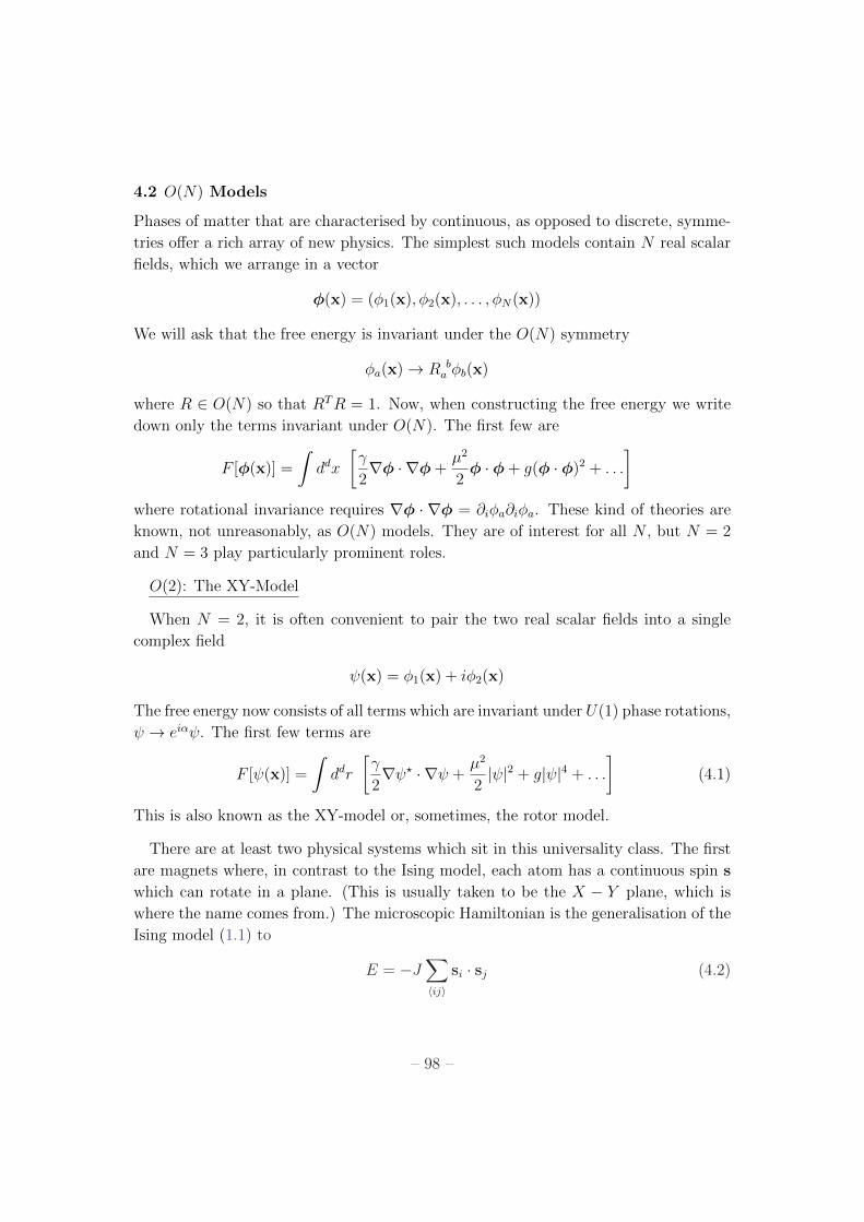
However, minimising the free energy does not determine the direction of �. We are

left with a space of ground states which is the sphere SN�1. Each point on the sphere,

parameterises the direction of � and has the same energy. The configuration in which

all the spins point like this:

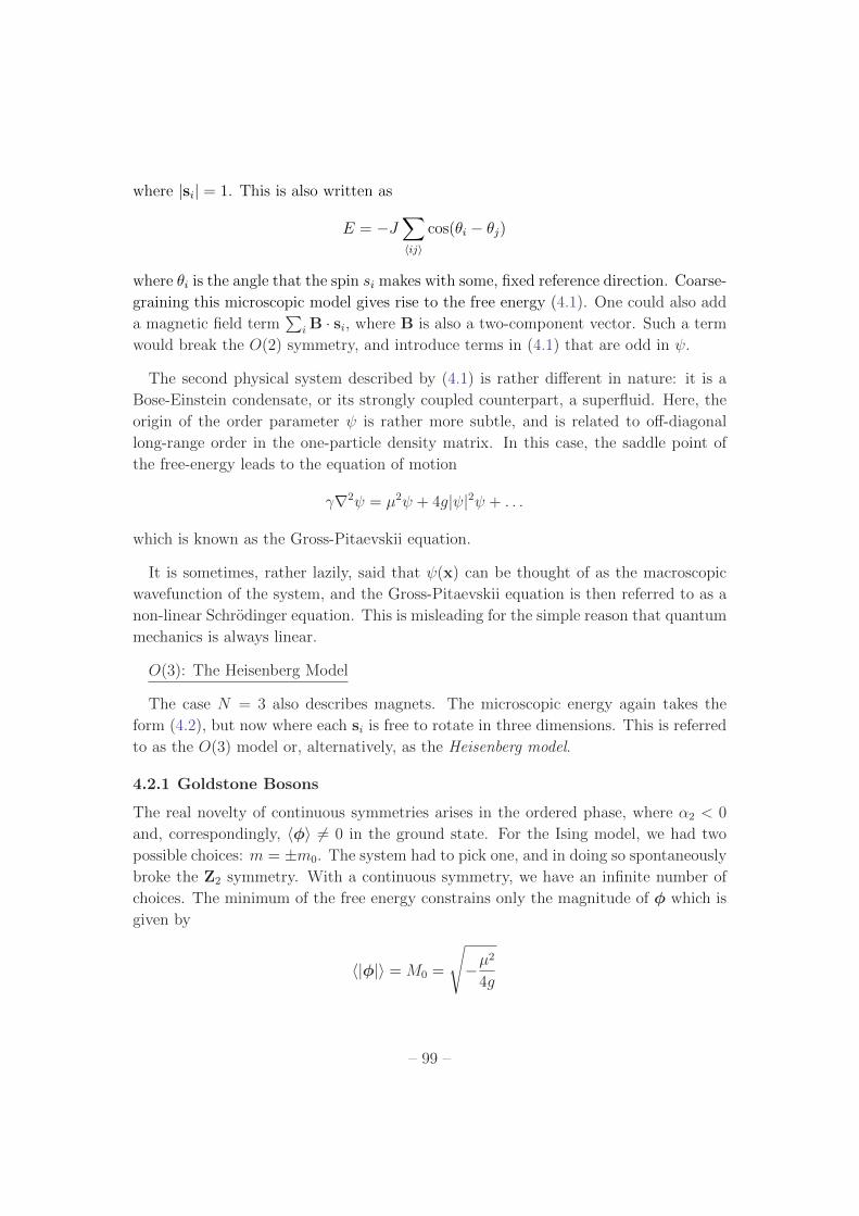
has the same energy as the configuration in which all the spins point like this:

This infinitely degenerate choice of ground states gives us something new. We can

consider configurations in which we stay within the space of ground states, but the

direction varies in space. For such configurations, the part of the free energy f(�) =µ

2

2

|�|2+ g|�|4+ . . . remains minimised, but we pick up contributions from the gradient

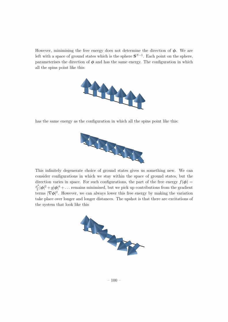
terms |r�|2. However, we can always lower this free energy by making the variation

take place over longer and longer distances. The upshot is that there are excitations of

the system that look like this

– 100 –

which can be made to cost an arbitrarily small amount of energy, by stretching the

winding over longer and longer distance scales.

These kind of excitations, which arise from the spontaneous breaking of continuous

symmetries, are known as Goldstone bosons, or sometimes Nambu-Goldstone bosons.

In the particular context of magnets, they are called spin waves.

There is a dizzying array of names for these kind of excitations, reflecting their

ubiquity and importance. In general, an excitation whose energy cost vanishes as the

wavelength goes to infinity is referred to as a soft mode or, alternatively, is said to

be gapless. These are to be contrasted with gapped excitations whose energy remains

finite in this limit. In the context of quantum field theory, “gapless” = “massless”, and

“gapped” = ”massive”, with the energy gap coming from E = mc2.

Gapless excitations often dominate the low-temperature behaviour of a system, where

they are the only excitations that are not Boltzmann suppressed. In many systems,

these gapless modes arise from the breaking of some symmetry. A particularly impor-

tant example, that we will not discuss in these lectures, are phonons in a solid. These

can be thought of as Goldstone bosons for broken translational symmetry.

The Symmetry Behind Goldstone Bosons

The intuitive idea described above can be placed on more rigorous footing in the form

of Goldstone’s theorem. This states that, in any system the spontaneous breaking of

a continuous symmetry gives rise to a gapless excitation, the eponymous Goldstone

boson. This can be stated in language of group theory.

For our O(N) model, the G = O(N) symmetry is broken by a choice of h�i to

H = O(N � 1). (To see this, note that if � = (M0

, 0, . . . , 0) then there is a surviving

O(N � 1) symmetry which acts on the on the string of zeros.) The space of ground

states has a group theoretic interpretation as the coset space

SN�1 =O(N)

O(N � 1)

This idea generalises. If a continuous symmetry G is spontaneously broken to H, then

the manifold of ground states is given by G/H. We get a Goldstone boson for each

broken symmetry generator, so the total number is

# Goldstone Bosons = dimG� dimH

For the O(N) model, G = O(N) and H = O(N�1) so the number of Goldstone modes

is then 1

2

N(N � 1)� 1

2

(N � 1)(N � 2) = N � 1, which is indeed the dimension of the

sphere SN�1.

– 101 –

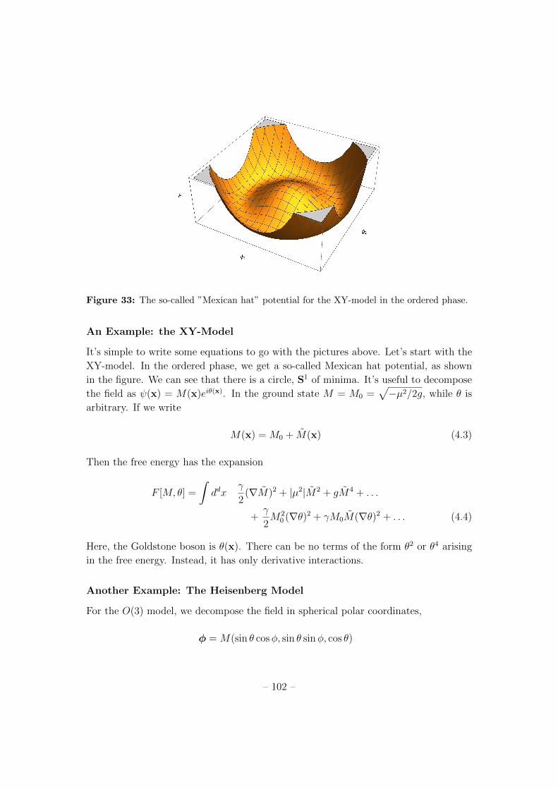
Figure 33: The so-called ”Mexican hat” potential for the XY-model in the ordered phase.

An Example: the XY-Model

It’s simple to write some equations to go with the pictures above. Let’s start with the

XY-model. In the ordered phase, we get a so-called Mexican hat potential, as shown

in the figure. We can see that there is a circle, S1 of minima. It’s useful to decompose

the field as (x) = M(x)ei✓(x). In the ground state M = M0

=p�µ2/2g, while ✓ is

arbitrary. If we write

M(x) = M0

+ M(x) (4.3)

Then the free energy has the expansion

F [M, ✓] =

Z

ddx�

2(rM)2 + |µ2|M2 + gM4 + . . .

+�

2M2

0

(r✓)2 + �M0

M(r✓)2 + . . . (4.4)

Here, the Goldstone boson is ✓(x). There can be no terms of the form ✓2 or ✓4 arising

in the free energy. Instead, it has only derivative interactions.

Another Example: The Heisenberg Model

For the O(3) model, we decompose the field in spherical polar coordinates,

� = M(sin ✓ cos�, sin ✓ sin�, cos ✓)

– 102 –

with ✓ 2 [0, ⇡) and � 2 [0, 2⇡). Once again, in the ordered phase we have M = M0

6= 0,

with ✓ and � arbitrary. Expanding M as (4.3), the free energy now takes the form

F [M, ✓,�] =

Z

ddx�

2(rM)2 + |µ2|M2 + gM4 + . . .

+�

2M2

0

⇥

(r✓)2 + sin2 ✓ (r�)2⇤+ . . . (4.5)

Here ✓ and � are the two Goldstone modes and, correspondingly, have only derivative

interactions. Note, however, that this time the Goldstone modes interact with each

other, as seen in the sin2 ✓ (r�)2 term.

The kinetic terms for the Goldstone bosons above take the form of the metric on

the two-sphere S2, i.e. ds2 = d✓2 + sin2 ✓d�2. This is no coincidence: the Goldstone

bosons describe fluctuations around the minima of the free energy F [�]. In the present

case, this set of minima is S2, and this geometry gets imprinted on the dynamics of the

Goldstone modes. We will explore this more in Section 4.3.

Correlation Functions

We saw in Section 2.2 that the quadratic term in the free energy is related (inversely) to

the correlation length ⇠. For Goldstone bosons this quadratic term necessarily vanishes

and so they have infinite correlation length.

This manifests itself in the correlation function, which decays as a power-law rather

than exponential. This is simplest to see in the XY-model. (We will discuss O(N)

models with N � 3 in more detail in Section 4.3.) The free energy (4.4) is

F [✓] =

Z

ddx�

2M2

0

(r✓)2 + . . .

where the higher order terms are all derivatives and will not a↵ect the discussion below.

To compute the correlation function h✓(x)✓(y)i, we can simply import the result (2.20).

(There are some subtleties in doing the path integral because ✓(x) is periodic, now

valued in [0, 2⇡) rather than R. These subtleties turn out not to be important here

but we will revisit them in Section 4.4.) The long distance behaviour is

h✓(x)✓(y)i = 1

�M2

0

Z

ddk

(2⇡)deik·(x�y)

k2

(4.6)

This is similar to the behaviour of the correlation function at the critical point. In-

deed, a critical point can be thought of as having gapless excitations. But there are

di↵erences.

– 103 –

First, the power-law decay at critical point requires some fine-tuning of a parameter;

we must pick the temperature to be exactly T = Tc

. In contrast, spontaneous symmetry

breaking is more robust, and we get power-law decay for all T < Tc

. In other words,

we have a phase with long range correlations, rather than just a point in the phase

diagram. (For T > Tc

, where there is no symmetry breaking, all modes still decay

exponentially as in the Ising model.)

The second di↵erence is that Goldstone bosons are much simpler to understand

than the gapless modes at a critical point. As we have seen, at critical points the

power-law decay of correlation functions su↵ers a correction due to integrating out

short distance modes, resulting in the critical exponent ⌘ 6= 0. There are no such

subtleties for Goldstone modes since all the dynamics is constrained by symmetry, and

the correlation function (4.6). There are two caveats to this statement, both of which

we will elaborate upon below. The first is that the simplicity only holds when T < Tc

;

when we sit at the critical point T = Tc

, things become interesting once again. The

second caveat is that we have to be above the lower critical dimension for the Goldstone

bosons to exist.

4.2.2 The d = 4� ✏ Expansion

At the critical temperature, T = Tc

, the O(N) models exhibit critical behaviour. The

mean field approach to the O(N) model gives the same answer as we saw for the N = 1

Ising field theory in previous sections. By now, you will not be surprised to learn that

these mean field exponents are not always correct. However, the system now does not

flow to the Ising critical point. Instead, they lie in a di↵erent universality class.

First, in d = 2 there are no critical points with G = O(N) symmetry. We’ll see why

in Section 4.2.3 and explore the physics more in Sections 4.3 and 4.4.

In d = 3, the theories flow to a di↵erent critical point for each N . The critical

exponents are known to be:

⌘ ⌫

MF 0 1

2

Ising 0.0363 0.6300

N = 2 0.0385 0.6719

N = 3 0.0386 0.702

where the other critical exponents, ↵, �, � and � all follow from the scaling relations

that we saw in Section 3.2.

– 104 –

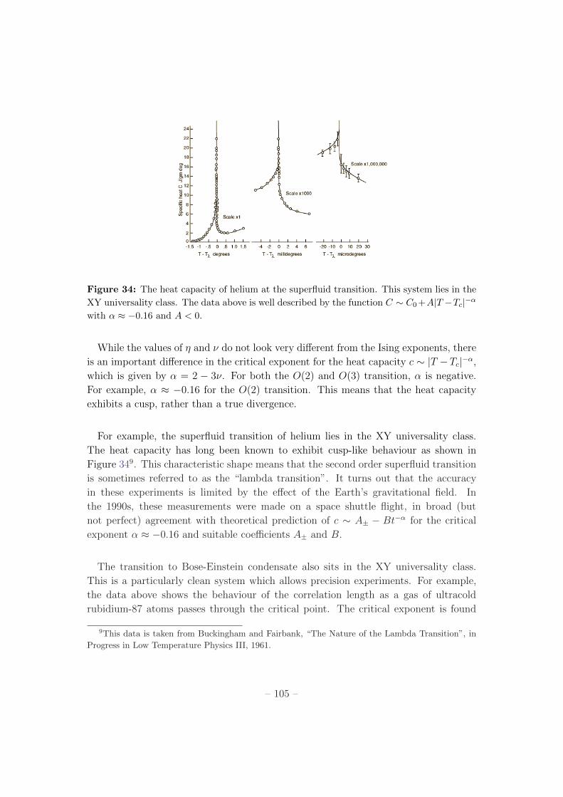
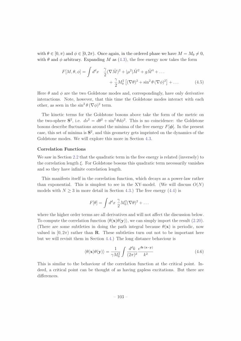
Figure 34: The heat capacity of helium at the superfluid transition. This system lies in the

XY universality class. The data above is well described by the function C ⇠ C0

+A|T �Tc

|�↵

with ↵ ⇡ �0.16 and A < 0.

While the values of ⌘ and ⌫ do not look very di↵erent from the Ising exponents, there

is an important di↵erence in the critical exponent for the heat capacity c ⇠ |T �Tc

|�↵,

which is given by ↵ = 2 � 3⌫. For both the O(2) and O(3) transition, ↵ is negative.

For example, ↵ ⇡ �0.16 for the O(2) transition. This means that the heat capacity

exhibits a cusp, rather than a true divergence.

For example, the superfluid transition of helium lies in the XY universality class.

The heat capacity has long been known to exhibit cusp-like behaviour as shown in

Figure 349. This characteristic shape means that the second order superfluid transition

is sometimes referred to as the “lambda transition”. It turns out that the accuracy

in these experiments is limited by the e↵ect of the Earth’s gravitational field. In

the 1990s, these measurements were made on a space shuttle flight, in broad (but

not perfect) agreement with theoretical prediction of c ⇠ A± � Bt�↵ for the critical

exponent ↵ ⇡ �0.16 and suitable coe�cients A± and B.

The transition to Bose-Einstein condensate also sits in the XY universality class.

This is a particularly clean system which allows precision experiments. For example,

the data above shows the behaviour of the correlation length as a gas of ultracold

rubidium-87 atoms passes through the critical point. The critical exponent is found

9This data is taken from Buckingham and Fairbank, “The Nature of the Lambda Transition”, in

Progress in Low Temperature Physics III, 1961.

– 105 –

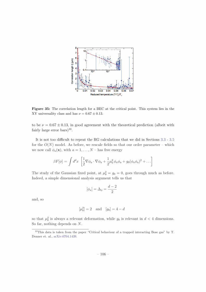
Figure 35: The correlation length for a BEC at the critical point. This system lies in the

XY universality class and has ⌫ = 0.67± 0.13.

to be ⌫ = 0.67 ± 0.13, in good agreement with the theoretical prediction (albeit with

fairly large error bars)10.

It is not too di�cult to repeat the RG calculations that we did in Sections 3.3 - 3.5

for the O(N) model. As before, we rescale fields so that our order parameter – which

we now call �a

(x), with a = 1, . . . , N – has free energy

�F [�] =

Z

ddx

1

2r�

a

·r�a

+1

2µ2

0

�a

�a

+ g0

(�a

�a

)2 + . . .

�

The study of the Gaussian fixed point, at µ2

0

= g0

= 0, goes through much as before.

Indeed, a simple dimensional analysis argument tells us that

[�a

] = ��

=d� 2

2

and, so

[µ2

0

] = 2 and [g0

] = 4� d

so that µ2

0

is always a relevant deformation, while g0

is relevant in d < 4 dimensions.

So far, nothing depends on N .

10This data is taken from the paper “Critical behaviour of a trapped interacting Bose gas” by T.

Donner et. al., arXiv:0704.1439.

– 106 –

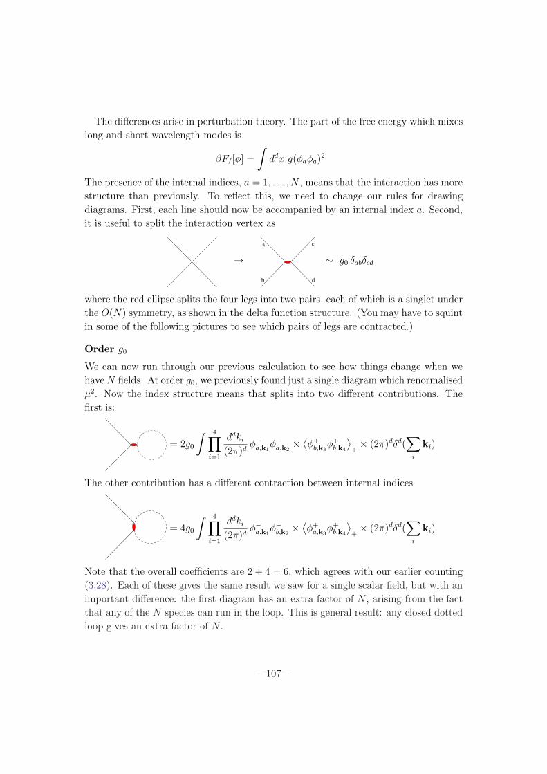
The di↵erences arise in perturbation theory. The part of the free energy which mixes

long and short wavelength modes is

�FI

[�] =

Z

ddx g(�a

�a

)2

The presence of the internal indices, a = 1, . . . , N , means that the interaction has more

structure than previously. To reflect this, we need to change our rules for drawing

diagrams. First, each line should now be accompanied by an internal index a. Second,

it is useful to split the interaction vertex as

!a

b

c

d

⇠ g0

�ab

�cd

where the red ellipse splits the four legs into two pairs, each of which is a singlet under

the O(N) symmetry, as shown in the delta function structure. (You may have to squint

in some of the following pictures to see which pairs of legs are contracted.)

Order g0

We can now run through our previous calculation to see how things change when we

haveN fields. At order g0

, we previously found just a single diagram which renormalised

µ2. Now the index structure means that splits into two di↵erent contributions. The

first is:

= 2g0

Z

4

Y

i=1

ddki

(2⇡)d��a,k1

��a,k2

⇥ ⌦�+

b,k3�+

b,k4

↵

+

⇥ (2⇡)d�d(X

i

ki

)

The other contribution has a di↵erent contraction between internal indices

= 4g0

Z

4

Y

i=1

ddki

(2⇡)d��a,k1

��b,k2

⇥ ⌦�+

a,k3�+

b,k4

↵

+

⇥ (2⇡)d�d(X

i

ki

)

Note that the overall coe�cients are 2 + 4 = 6, which agrees with our earlier counting

(3.28). Each of these gives the same result we saw for a single scalar field, but with an

important di↵erence: the first diagram has an extra factor of N , arising from the fact

that any of the N species can run in the loop. This is general result: any closed dotted

loop gives an extra factor of N .

– 107 –

The rest of the calculation proceeds as in Section 3.4.1. We find that, at this order,

we have a renormalisation of the quadratic term given by

µ2

0

! µ0 2 = µ2

0

+ 4(N + 2)g0

Z

⇤

⇤/⇣

ddq

(2⇡)d1

q2 + µ2

0

This agrees with our earlier result (3.30) when N = 1.

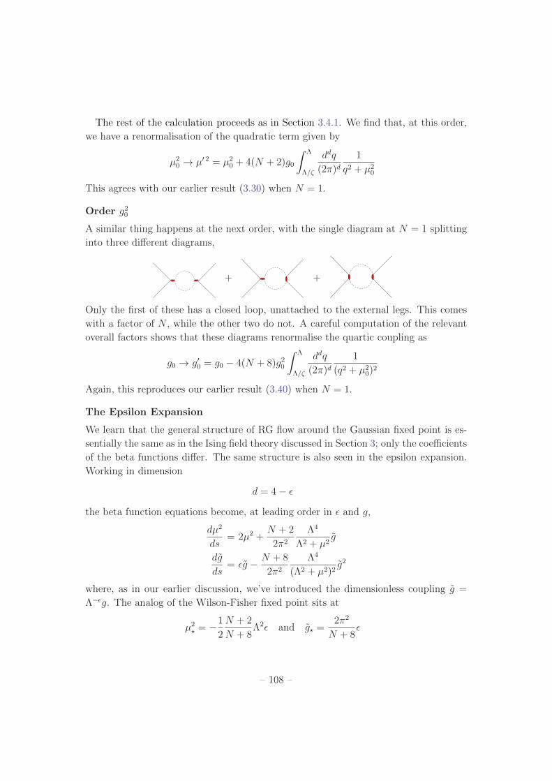
Order g20

A similar thing happens at the next order, with the single diagram at N = 1 splitting

into three di↵erent diagrams,

+ +

Only the first of these has a closed loop, unattached to the external legs. This comes

with a factor of N , while the other two do not. A careful computation of the relevant

overall factors shows that these diagrams renormalise the quartic coupling as

g0

! g00

= g0

� 4(N + 8)g20

Z

⇤

⇤/⇣

ddq

(2⇡)d1

(q2 + µ2

0

)2

Again, this reproduces our earlier result (3.40) when N = 1.

The Epsilon Expansion

We learn that the general structure of RG flow around the Gaussian fixed point is es-

sentially the same as in the Ising field theory discussed in Section 3; only the coe�cients

of the beta functions di↵er. The same structure is also seen in the epsilon expansion.

Working in dimension

d = 4� ✏

the beta function equations become, at leading order in ✏ and g,

dµ2

ds= 2µ2 +

N + 2

2⇡2

⇤4

⇤2 + µ2

g

dg

ds= ✏g � N + 8

2⇡2

⇤4

(⇤2 + µ2)2g2

where, as in our earlier discussion, we’ve introduced the dimensionless coupling g =

⇤�✏g. The analog of the Wilson-Fisher fixed point sits at

µ2

?

= �1

2

N + 2

N + 8⇤2✏ and g

?

=2⇡2

N + 8✏

– 108 –

Around this fixed point, the linearised beta functions take the form

d

ds

�µ2

�g

!

=

2� N+2

N+8

✏ C

0 �✏

!

�µ2

�g

!

where the o↵-diagonal entry is C = N+2

2⇡

2 ⇤2 + (N+2)

2

4⇡

2(N+8)

⇤2✏. This does not a↵ect the

eigenvalues which are given by the diagonal entries,

�t

= 2� N + 2

N + 8✏+O(✏2) and �

g

= �✏+O(✏2)

The interacting fixed point has one relevant and one irrelevant direction, just like for

the Ising model. To leading order in ✏, the critical exponents are

↵ =4�N

2(N + 8)✏ , � =

1

2� 3

2(N + 8)✏ , � = 1 +

N + 2

2(N + 8)✏

and

⌫�1 = 2� N + 2

N + 8✏ (4.7)

Meanwhile � = 3 + ✏ is independent of N , and the anomalous dimension turns out to

be ⌘ = (N + 2)✏2/2(N + 8)

4.2.3 There Are No Goldstone Bosons in d = 2

We learned in Section 1 that field theories have a lower critical dimension, in which

the ordered phase ceases to exist. For theories characterised by any discrete symmetry,

such as the Z2

of the Ising field theory, this lower critical dimension is dl

= 1. As we

explained in (1.3.3), the lack of an ordered phase in d = 1 dimensions can be traced to

the existence of domain walls.

The story is di↵erent when we have continuous symmetries. Now there are no domain

walls because the space of ground states is continuously connected. However, there is

a more prominent phenomena which means that the lower critical dimension is raised

to dl

= 2.

An Example: the XY model

The lack of ordered phase in d = 2 dimensions arises due to the presence of the would-

be Goldstone modes. This is simplest to explain in the XY model. Let’s sit in the

broken phase and focus only on the Goldstone bosons. We must pick a ground state

– 109 –

for ✓: this is the essence of spontaneous symmetry breaking. Let’s choose h✓(x)i = 0.

We now look at fluctuations around this ground state,

h[✓(x)� ✓(0)]2i = 2h✓(x)2i � 2h✓(x)✓(0)i (4.8)

From the correlation function (4.6), the long distance behaviour is

h✓(x)✓(0)i = 1

�M2

0

Z

⇤ ddk

(2⇡)de�ik·x

k2

⇠

8

>

>

<

>

>

:

⇤d�2 � r2�d d > 2

log(⇤r) d = 2

r � ⇤�1 d = 1

(4.9)

with r = |x|.

We see that there is a qualitative di↵erence between d > 2 and d 2. For d > 2,

the two point correlator h✓(x)✓(0)i decays to a constant as r ! 1. This constant is

cancelled by the other term in (4.8), which means that the phase returns to its original

value h✓i = 0.

In contrast, for d 2, the fluctuation of the phase grows indefinitely as we go to

larger distances. You may have thought that you had placed the system in a fixed

ground state, but the thermal fluctuations of the Goldstone mode mean that it doesn’t

stay there. The interpretation is that there is no ordered phase with h�i 6= 0 in d = 2

dimensions or below.

This is a general result, known as the Mermin-Wagner theorem. A continuous sym-

metry cannot be spontaneously broken in d = 2 dimensions or below: there are no

Goldstone bosons in d = 2 dimensions.

This leaves us with a delicate question. The existence of the gapless Goldstone

modes was predicated on the idea of spontaneous symmetry breaking. But for d 2

dimensions, no such symmetry breaking happens. What, then, is the resulting physics?

In d = 1, the physics is straightforward: there are no gapless modes. As before, this

can also be understood in the language of quantum mechanics, where the spectrum

of a particle moving on SN�1 is discrete and gapped. For d = 2, the physics is more

interesting. It turns out that the answer is somewhat di↵erent for O(N) models with

N � 3 and for the XY-model with N = 2. We will discuss the fate of the Goldstone

modes for each of these in Sections 4.3 and 4.4 respectively.

– 110 –

4.3 Sigma Models

We have still to understand the fate of the Goldstone bosons in d = 2 dimensions. In

this section, we will tell their story. As a spin-o↵, we will see that we also a get a new

handle on the critical point in d = 3 dimensions.

We place ourselves firmly in the ordered phase, with T < Tc

. Mean field consider-

ations tell us that h|�|i 6= 0, leaving us with a space of possible ground states which

is identified with the sphere SN�1. As we saw in Section 4.2.1, fluctuations in the

directions parallel to the SN�1 have only power-law decay; these are the Goldstone

modes. In contrast the “longitudinal” fluctuation, in which �� ⇠ h�i, acts very much

like in the Ising model and has exponential decay with a correlation length ⇠ 6= 0. This

suggests that the long distance dynamics is dominated purely by the Goldstone modes.

Here we will study the theory of these Goldstone modes. First, rather than working

with � · � = M2

0

, we rescale the field �(x) to a new field, n(x) which has unit length,

n · n = 1 (4.10)

For now, we will keep the dimension d arbitrary. The free energy is given by

F [n] =

Z

ddx1

2e2rn ·rn (4.11)

where the coe�cient e2 = 1/�M2

0

is the price that we pay for rescaling n to be a unit

vector. The free energy (4.11) looks like that of a free theory; all the interactions come

from the constraint (4.10) which say that the fields n(x) must lie on the unit sphere

SN�1.

The theory defined by (4.11), together with the constraint (4.10), lies in a class

of theories referred to as non-linear sigma models. These are theories in which the

fields can be viewed as coordinates on some manifold M. In the present context, this

manifold is M = SN�1.

We would like to understand the path integral for the sigma model. Schematically,

this can be written as

Z =

Z

Dn ��

n(x)2 � 1�

exp

✓

� 1

2e2

Z

ddx rn ·rn

◆

(4.12)

Here we’ve imposed the constraint through a delta function. Note that the only coef-

ficient in the game is e2; this will play the role of our coupling constant. Recall that,

long ago, before we grew up and set � = 1, we used to write the partition function

as e��F . Comparing to this form suggests that e2 can be viewed as temperature, with

large e2 corresponding to high temperature. This interpretation will be useful later.

– 111 –

We can do some simple dimensional analysis. The field n(x) must be dimensionless

since it obeys the constraint (4.10). So,

[e2] = 2� d (4.13)

In particular, e2 is dimensionless in d = 2. Here the theory is weakly coupled when

e2 ⌧ 1, in the sense that field configurations n(x) with wild spatial variations are

suppressed in the path integral. Before our rescaling, this corresponds to the case where

� parameterise a large SN�1 sphere. In contrast, when e2 � 1 these configurations

are unsuppressed and the theory is strongly coupled; in this case the � parameterise a

small sphere.

It is possible to write the sigma model in a more explicit form. We can decompose

the vector n as

n(x) = (~⇡(x), �(x))

where ~⇡(x) is an (N � 1)-dimensional vector and �(x) is given by

�(x)2 = 1� ~⇡(x) · ~⇡(x)which ensures that the fields sit on the ground state manifold n ·n = 1. The free energy

is then given by

F [~⇡] =

Z

ddx1

2e2[r~⇡ ·r~⇡ +r�r�]

=

Z

ddx1

2e2

r~⇡ ·r~⇡ +(~⇡ ·r~⇡)21� ~⇡2

�

(4.14)

This form of the sigma model does not have any constraint; it is an interacting theory of

the Goldstone modes ~⇡(x). However, we have paid a price: only an O(N�1) symmetry

is now manifest in the free energy, rather than the full O(N) symmetry. This is because

we have had to make a choice of which of the redundant n variables to eliminate in

order to solve the constraint (4.10). Related to this, our free energy (4.14) is now only

valid as long as �(x) 6= 0 anywhere, in which case the second term would diverge.

This is because the ~⇡ fields are coordinates on the space SN�1 and it is impossible to

introduce coordinates which are well behaved over the entire manifold.

As an aside: the name “sigma model ” is, obviously, completely uninformative. It

has its roots in particle physics where a theory of this type describes the interactions

of pions. Strangely, the eponymous “sigma” meson is the one particle not described by

the sigma-model; it is analogous to the longitudinal mode �(x) which is determined in

terms of the ~⇡ fields in our description above.

– 112 –

4.3.1 The Background Field Method

We would like to perform a renormalisation group analysis on the sigma model. There

are a number of ways to proceed. First, we could Taylor expand the second term in the

free energy for small ~⇡. This would result in an infinite tower of interactions. We could

then restrict attention to the first few, and do the kind of Wilsonian RG treatment

we’ve seen before. This method works, but it butchers the underlying geometry and,

in doing so, disguises what’s really going on.

Instead, there is a better approach, first introduced in this context by Polyakov,

called the background field method. First, suppose that n(x) takes some profile which

varies slowly in space,

na(x) = na(x)

This profile must obey n · n = 1. This will play the role of our long wavelength modes.

On top of this background, we want to introduce short wavelength modes which

change rapidly in space. To parameterise these modes, we first introduce frame fields.

These are a basis of N � 1 unit vectors ea↵

(x), with a = 1, . . . , N and ↵ = 1, . . . N � 1,

which are orthogonal to na(x),

na(x)ea↵

(x) = 0 8 ↵ and ea↵

(x)ea�

(x) = �↵�

(4.15)

The frame fields are, like na, slowly varying in space. There is an ambiguity in the

definition of these frame fields; we can always rotate them by a local O(N � 1) trans-

formation and we will still have a good set of frame fields.

The short wavelength modes sit on top of our original field n(x) and fluctuate in the

direction of the frame fields. We call these �↵

(x), and write the full configuration as

na(x) = na(x) (1� �(x)2)1/2 +N�1

X

↵=1

�↵

(x)ea↵

(x) (4.16)

By construction, this configuration still satisfies the constraint (4.10). This is morally

equivalent to our previous Fourier space decomposition � = �� + �+

, but now in real

space. We will integrate out the short wavelength modes � and determine their e↵ect

on the long wavelength mode n.

– 113 –

Integrating out Short Wavelengths

We have a short calculation ahead of us. Our plan is to expand the free energy to

quadratic order in the short wavelength fields �↵

(x) and then integrate them out, in

exactly the same way that we integrated out the Fourier modes �+

previously. We will

then interpret this in terms of an e↵ective free energy for the long wavelength fields na

and, in particular, in terms of a renormalisation of the coupling e2.

First, we have

rna = rna (1� �2)1/2 + nar(1� �2)1/2 +r(�↵

ea↵

)

= rna(1� 1

2�2)� na�

↵

r�↵

+r(�↵

ea↵

) +O(�2)

The gradient term then becomes

(rna)2 = (rna)2(1� �2) + (r�↵

)2 + �↵

��

rea↵

rea�

+ 2rnar(�↵

ea↵

) +O(�3)

where we have used the identities (4.15). One of the cross-terms vanishes by dint of

the fact that nana = 1 so that narna = 0.

Our partition function is now

Z =

Z

Dn �(n2 � 1) e�1

2e2

Rd

dx(rn)

2

Z

D� e�1

2e2

Rd

dx(r�)

2

e�FI [n,�]

where the interaction between na and �↵

are captured in

FI

[na,�↵

] =1

2e2

Z

ddxh

� �2(rna)2 + �↵

��

rea↵

rea�

+ 2rnar(�↵

ea↵

)i

As previously, we interpret the functional integral over � as computing the expectation

value of e�FI using the probability distribution exp(� 1

2e

2

R

ddx (r�)2). In other words,

Z =

Z

Dn �(n2 � 1) e�1

2e2

Rd

2x(rn)

2 ⌦

e�FI [n,�]↵

The expectation value can be Taylor expanded,

⌦

e�FI [n,�]↵

= 1� hFI

i+ 1

2hF 2

I

i+ . . . (4.17)

As usual, the renormalisation group will generate many terms when we integrate out

�. Our interest is in how the leading order kinetic terms (rn)2 are a↵ected; all other

terms will turn out to be irrelevant. At leading order, it is su�cient to focus on hFI

i.(Given the term linear in �, one might wonder if such a term can be generated from

– 114 –

hF 2

I

i; a closer inspection shows that this in fact gives rise only to terms like (rn)4.)

We have

hFI

i = 1

2e2

Z

ddx���

↵�

(rna)2 +rea↵

rea�

� h�↵

(x)��

(x)i (4.18)

where we’ve used the fact that h�(x)i = 0 to lose the linear term. The correlator that

we want takes the same form that we calculated in previous sections. (See, for example,

(2.21).)

h�↵

(x)��

(x)i = e2�↵�

Id

where

Id

=

Z

⇤

⇤/⇣

ddq

(2⇡)d1

q2

Here we’ve introduced the limits on the integral to reflect the fact that, as in our earlier

RG analysis, the short wavelength modes – which are here �↵

(x) – have support only

in ⇤/⇣ < k < ⇤. The integral is simple to perform; we have

Id

=⌦

d�1

(2⇡)d⇤d�2 ⇥

8

>

>

<

>

>

:

⇣ � 1 d = 1

log ⇣ d = 2

1� ⇣2�d d � 3

where ⌦d�1

is the area of the unit sphere Sd�1. Substituting this into (4.18), it is

clear that the first term corrects the kinetic term in the sigma model. But what of the

second term? Using the fact that the correlator is proportional to �↵�

, it takes the form

rea↵

rea↵

. We can massage this into the form we need using some identities. Between

then, the fields (na, ea↵

) provide an orthonormal basis of RN . Inverting this, we have

nanb + ea↵

eb↵

= �ab (4.19)

Using this, we can write

rea↵

rea↵

= rea↵

reb↵

(nanb + ea�

eb�

)

But since naea↵

= 0, we have narea↵

= �(rna)ea↵

so

rea↵

rea↵

= ea↵

eb↵

(rna)(rnb) + (ea�

rea↵

)(eb�

reb↵

)

= rnarna + (ea�

rea↵

)(eb�

reb↵

)

where, in going to the second line, we’ve used (4.19) again, together with the fact that

narna = 0. The first term is just what we want; the second term is a new term that we

can add to the sigma model and will be generated by RG. It is related to the geometric

concept of torsion; it turns out to be irrelevant and we will not discuss it further here.

– 115 –

Both terms in (4.18) now give a contribution to (rna)2; the first is ��↵�

�↵� =

�(N � 1); the second is simply +1. The upshot of this is that the hFI

i includes the

term

hFI

i = (2�N)Id

Z

ddx1

2(rna)2

We now exponentiate this so that, to the order we’re working at, (4.17) becomes

he�FI i = e�hFIi. This gives us an e↵ective free energy for the long wavelength field

n,

F [n] =

Z

ddx1

2e0 2rn ·rn

with

1

e0 2=

1

e20

+ (2�N)Id

Usually there are two further steps in the RG programme. First, we need to rescale

our momentum cut-o↵ back up to ⇤, and in doing so rescale all length by 1/⇣. This

proceeds as before. The second step, advertised in Section 3, is to rescale the fields

so that the kinetic term is canonically normalised. This step is not for us, since the

normalisation of the kinetic term is the only coupling we have. Instead, the fields are

normalised correctly by imposing the constraint (4.10). The upshot is that we have the

running coupling constant

1

e2(⇣)= ⇣d�2

✓

1

e20

+ (2�N)Id

◆

(4.20)

The first term comes from the naive dimensional analysis [e2] = 2 � d that we saw

in (4.13); the second term is the one-loop correction from integrating out the high

momentum modes.

Note that this second term vanishes when N = 2. This reflects the fact that the

Goldstone boson in the XY-model is free; this can be seen in (4.4) where there are no

interaction terms. Interesting things happen in the XY-model but we will postpone

discussion to Section 4.4. In contrast, for N � 3 the Goldstone bosons are interacting,

as can be seen for the O(3) model in (4.5), and this drives the running of the coupling

constant.

– 116 –

orderedphase

d=1d=2

d>2

disordered phase

(g)β

e2

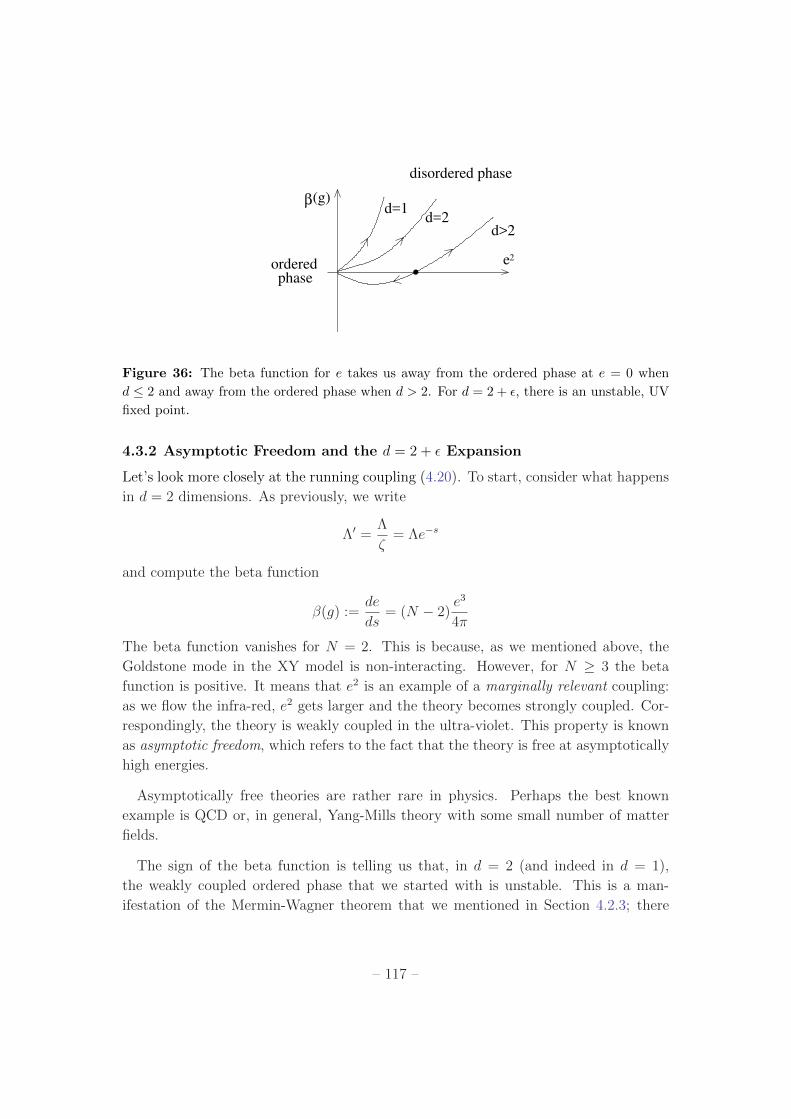
Figure 36: The beta function for e takes us away from the ordered phase at e = 0 when

d 2 and away from the ordered phase when d > 2. For d = 2 + ✏, there is an unstable, UV

fixed point.

4.3.2 Asymptotic Freedom and the d = 2 + ✏ Expansion

Let’s look more closely at the running coupling (4.20). To start, consider what happens

in d = 2 dimensions. As previously, we write

⇤0 =⇤

⇣= ⇤e�s

and compute the beta function

�(g) :=de

ds= (N � 2)

e3

4⇡

The beta function vanishes for N = 2. This is because, as we mentioned above, the

Goldstone mode in the XY model is non-interacting. However, for N � 3 the beta

function is positive. It means that e2 is an example of a marginally relevant coupling:

as we flow the infra-red, e2 gets larger and the theory becomes strongly coupled. Cor-

respondingly, the theory is weakly coupled in the ultra-violet. This property is known

as asymptotic freedom, which refers to the fact that the theory is free at asymptotically

high energies.

Asymptotically free theories are rather rare in physics. Perhaps the best known

example is QCD or, in general, Yang-Mills theory with some small number of matter

fields.

The sign of the beta function is telling us that, in d = 2 (and indeed in d = 1),

the weakly coupled ordered phase that we started with is unstable. This is a man-

ifestation of the Mermin-Wagner theorem that we mentioned in Section 4.2.3; there

– 117 –

are no Goldstone bosons in d 2. Unfortunately to really understand the infra-red

physics in these low dimensions we will have to figure out how to deal with the strongly

interacting theory. We will introduce a particularly useful approach in Section 4.3.3.

In higher dimensions, say d = 3, the beta function is negative. This means that the

sigma-model flows towards weak coupling in the infra-red, telling us that the ordered

phase is stable.

However, there is now something new we can do. We can look at what happens in

dimension

d = 2 + ✏

Here the beta function takes the form

de

ds= � ✏

2e+ (N � 2)

e3

4⇡⇤✏

This has a fixed point that lies within the remit of perturbation theory, namely

e2?

=2⇡✏

N � 2⇤�✏ (4.21)

However, in contrast to the story of Section 4.2, this is now a UV fixed-point, rather

than an IR fixed point. How should we interpret this?

To understand this, let’s recap the story so far. The O(N) model, with unconstrained

fields �, has a Wilson-Fisher fixed point in dimension d = 3. This has one relevant

deformation which is, roughly speaking, �2. If we turn on this relevant deformation

with negative sign, we flow to the ordered phase which is described by our sigma model.

What we’re seen above is this story in reverse. Starting from the ordered phase,

described by the sigma model, we have managed to claw our way back up the RG flow

to find a UV fixed point, at least in dimensions d = 2 + ✏. It is natural to identify

this with the Wilson-Fisher point, viewed through di↵erent eyes. This provides us with

a di↵erent handle on the O(N) Wilson-Fisher fixed points for N � 3; we can either

approach them from above using the d = 4 � ✏ expansion, or from below using the

d = 2 + ✏ expansion.

To extract the critical exponent ⌫, we need to understand how e2 is related to the

temperature. From our definition of the path integral (4.12), we see that 1/e2 sits in

the exponent where � would sit in a usual partition function. This motivates us to

– 118 –

identify e2 with temperature T and the fixed point e2?

with the critical temperature T?

.

We then linearise about the fixed point by writing e2 = e2?

+ �e2 to find

d(�e2)

ds= +✏ �e2

This gives �t

= ✏ and, correspondingly, the critical exponent

⌫ =1

✏(4.22)

independent of N . To compute the critical exponent ⌘, one could add the interac-

tionR

ddx B · n(x) or, alternatively, extract the anomalous dimension of n from the

calculation above. One finds that

⌘ =✏

N � 2

The d = 2 + ✏ expansion does not give great results if we just go ahead and plug in

✏ = 1. But then, there is little reason that it should! For example, for N = 3, we can

compare the best known results with mean field, and with the d = 4� ✏ and d = 2+ ✏

expansions, where we work to first order and plug in ✏ = 1. We have

⌘ ⌫

MF 0 1

2

d = 4� ✏ 0 0.61

d = 2 + ✏ 1 1

Actual 0.0386 0.702

Nonetheless, there is some utility in having two expansion parameters, coming from

di↵erent ends. By going to higher powers in ✏, one can try to use sophisticated matching

techniques to join together the two expansions and get a better handle on the values

of the critical exponents for d = 3.

4.3.3 Large N

So far, we have seen that the dynamics of interacting Goldstone modes (i.e. N � 3)

becomes strongly coupled in d = 2 dimensions. But we have yet to figure out what

actually happens.

Questions like this are typically hard. As e2 ! 1, it naively appears that all field

configurations contribute equally to the path integral, no matter how wildly they vary

and how far they are from the saddle point. We have very few techniques to deal with

such situations. Often we have to turn to some hidden and surprising symmetry, or to

some unusual limit where the theory is soluble.

– 119 –

In the present case, it turns out that such a limit exists: it is N ! 1. To proceed,

we first rewrite the delta-function in the path integral (4.12) as

Z =

Z

Dn �(n2 � 1) exp

✓

� 1

2e20

Z

ddx rn ·rn

◆

=

Z

DnD� exp

✓

� 1

2e20

Z

ddx rn ·rn� i

2e20

Z

ddx � (n · n� 1)

◆

(4.23)

Here the field �(x) plays the role of a Lagrange multiplier; integrating it out gives us

back the delta-function, imposing the field constraint n2 = 1.

Now, however, we’re left with a free energy which is quadratic in the n. Instead of

integrating out �, we can instead integrate out n. This gives us

Z =

Z

D� det �N/2

��r2 + i�(x)�

exp

✓

i

2e20

Z

ddx �

◆

Here the determinant of the di↵erential operator should be viewed, in the usual way,

as the product of all its eigenvalues, with a truncation associated to the UV cut-o↵

⇤, reflecting the fact that the eigenfunctions can’t oscillate at high frequencies. This

determinant will, in general, be a complicated function of �, and it does not look as if

we are any closer to evaluating the path integral. We can, however, use the standard

“log det = tr log” identity to write the partition function as

Z =

Z

D� exp

✓

�N

2tr log

��r2 + i��

+i

2e20

Z

ddx �

◆

(4.24)

The factor of N in front of the first term is what gives us hope because, in the limit

N ! 1, this term is then crying out to be evaluated by saddle point. However, we’re

still left with the second term. We can only apply the saddle point technique to this too

if we scale the coupling e20

with N in a particular way. Specifically, we send N ! 1,

keeping e20

N fixed.

The path integral (4.24) is then dominated by the minimum. We use the identity

� tr logX = trX�1�X, to find that the saddle point is

N

2G(x,x) =

1

2e20

(4.25)

where G(x,x0) is the Green’s function for the operator (�r2 + i�(x)). This equation

looks somewhat foreboding, but is rather simple in Fourier space. First, we look for

constant solutions, of the form

�(x) = �iµ2

– 120 –

Note the factor of i; our saddle point sits on the complex plane, but is nonetheless still

applicable. The saddle point (4.25) then becomes simpler in Fourier space: we haveZ

⇤ ddk

(2⇡)d1

k2 + µ2

=1

e20

N(4.26)

where we’ve explicitly included the UV cut-o↵ ⇤ in the integral. This equation should

now be viewed as an equation for µ2.

Large N in d = 2

It is perhaps no surprise by now to learn that solutions to (4.26) depend on the dimen-

sion d. Our main concern was with the fate of the Goldstone bosons in d = 2. Here

the integral gives us

1

4⇡log

✓

⇤2 + µ2

µ2

◆

=1

e20

N(4.27)

If we start with a weakly coupled theory in the UV, e20

N ⌧ 1, then we can self-

consistently assume that µ ⌧ ⇤ to find the solution

µ ⇡ ⇤e�2⇡/e

20N (4.28)

This simple formula is interesting for several reasons. First, let’s understand the phys-

ical interpretation of setting � = �iµ2 6= 0. Referring back to (4.23), we see that it

induces an e↵ective quadratic term for n2 in the free energy. This kind of term was

supposed to be prohibited by Goldstone’s theorem, but here we see that it is generated

– at least in the large N limit – by thermal fluctuations in d = 2 dimensions. This

means that the Goldstone bosons in d = 2 are no longer gapless. Correspondingly, if

we compute their correlator using (4.23), we will see that it decays exponentially, with

a finite correlation length given by ⇠ ⇠ 1/µ.

The second interesting fact about (4.28) is that the dynamically generated scale µ is

exponentially smaller than the UV cut-o↵ ⇤. Indeed, the function e�1/x has the lovely

property that its Taylor expansion around x = 0 vanishes at every order in x. This

means that the gap µ will not show up in any order in perturbation theory in e0

. We

say that it is a non-perturbative e↵ect.

Although the calculation we presented above is valid for N � 1, it turns out that

the conclusions hold for all N � 3; that is, for any theory of interacting Goldstone

bosons in d = 2 dimensions. This means that there is no phase transition for O(N)

models with N � 3 in d = 2 dimensions. As we lower the temperature, mean field

theory suggests that we enter an ordered phase with gapless excitations, but this is

misleading: instead, thermal fluctuations destroy both the order and gapless modes.

– 121 –

The discussion above carries over directly to quantum field theory, where non-linear

sigma models in d = 1+1 dimensions are also of great interest. Here the interpretation

of the calculation is that the Goldstone modes – which appear to be massless in the

classical action – get a mass due to quantum e↵ects. If one didn’t think carefully about

the meaning of quantum field theory this appears miraculous because the sigma-model

in d = 1+1 dimensions has only a dimensionless coupling e20

. Yet somehow, the theory

generates a mass out of this dimensionless coupling, a phenomenon that is known as

dimensional transmutation. The reason that this is mathematically possible is because

a quantum field theory, like is statistical counterpart, is not defined by the classical

action (or free energy) alone. It also requires a UV cut-o↵ ⇤. And, as we see in (4.28),

it is this UV cut-o↵ which provides the dimensional scale for the mass.

Finally, I should mention that if you can do a calculation like the one above for Yang-

Mills in d = 3 + 1 dimensions (or, indeed, in d = 4 dimensions) then fame and fortune

awaits. The massless gauge bosons that appear in the classical action are strongly

believed to get a mass through quantum e↵ects, yet this remains to be proven. This

is the famous “Yang-Mills mass gap” problem. The O(N) sigma model in d = 1 + 1

dimensions provides a useful analogy for how this might happen.

Large N in d > 2

We can also ask if our large N analysis can shed any light on the Wilson-Fisher fixed

point in d = 3. (Or, if you’re willing for dimensions to wander, in 2 < d < 4.) Here we

find something interesting. The saddle point equation (4.26) has di↵erent behaviour

for 2 < d < 4 and for d > 4,

1

e20

N=

Z

⇤ ddk

(2⇡)d1

k2 + µ2

⇠(

⇤d�2 � µ2⇤d�4 d � 4

⇤d�2 � µd�2 2 < d < 4(4.29)

where we haven’t been careful about the coe�cients in front of either term, except to

stress that the second term comes with a negative sign relative to the first. (We also

analysed the behaviour of this integral in (2.13), but there only kept the leading term.)

This equation now has rather di↵erent behaviour than the corresponding equation

(4.27) in d = 2. In particular, when the theory is weakly coupled at the cut-o↵ scale,

in the sense that

e20

N . ⇤2�d

there are no solutions to (4.29) for µ2. In this case, one finds that the saddle point of

the free energy actually arises when n gets an expectation value. In other words, it’s

reconfirming our expectation that the low-energy physics is that of Goldstone bosons.

– 122 –

In contrast, as the theory becomes more strongly coupled at the cut-o↵ scale, there

is a critical value

e2?

N ⇠ ⇤2�d

at which solutions to (4.29) for µ start to appear.

As in the previous section, we identify the deviation from e2?

with the temperature,

T � Tc

⇠ e2 � e2?

We can then ask how the correlation length ⇠ ⇠ 1/µ diverges as we approach this

critical coupling from above. Here the story is di↵erent for 2 < d < 4 and d > 4,

because of the di↵erent behaviour of the subleading term in (4.29). For 2 < d < 4, we

have

T � Tc

⇠ ⇠2�d

which gives the critical exponent

⌫ =1

d� 2

Rather wonderfully, this agrees precisely (for all 2 < d < 4) with the result of our

d = 2+ ✏ expansion (4.22), and with the large N limit of our result from the d = 4� ✏

expansion (4.7). Indeed, this result is exact in the N ! 1 limit and can be used as

the starting point for a 1/N expansion

Meanwhile, when d > 4 we can read o↵ the behaviour from (4.29); we have

T � Tc

⇠ ⇠�2 ) ⌫ =1

2

This, of course, is the mean field value that we expect.

4.4 The Kosterlitz-Thouless Transition

The Mermin-Wagner theorem means that any system with a continuous symmetry has

no ordered phase in d = 2 dimensions. As we saw in the previous sections, for the

O(N) model with N � 3, the would-be Goldstone modes are interacting and become

gapped as a result of the thermal fluctuations. This means that these models do not

exhibit a phase transition as the temperature is lowered.

– 123 –

However, the results of the previous section do not hold for the XY model with

N = 2. In this case, the sigma-model coupling does not run, and the system remains

gapless at low temperatures. As we will now see, the resulting physics is rather more

subtle and interesting.

The first surprise is that the d = 2 XY model does exhibit a phase transition as

the temperature is lowered. However, it is somewhat di↵erent from the kind of phase

transitions that we have met so far. In particular, as we saw in Section 4.2.3, thermal

fluctuations mean that there can be no spontaneous breaking of continuous symmetry

in d = 2 and, correspondingly, there is no local order parameter that distinguishes the

two phases. Instead, that task falls on the correlation function.

In the high temperature phase, we work with the complex field . The free energy

has a quadratic term µ2| |2 and, as we’ve now seen many times (starting in (2.29)) the

correlation function decays exponentially

h †(x) (0)i = e�r/⇠

pr

(4.30)

with ⇠ ⇠ 1/µ2. In contrast, in the low temperature phase we have µ2 < 0 and, as

we described in Section 4.2, we can write = Mei✓, with the long distance physics

dominated by ✓. To leading order, we can write the free energy as

F [✓] =1

2e2

Z

d2x (r✓)2 (4.31)

The low temperature phase corresponds to e2 ⌧ 1.

The correlation function for this Goldstone mode exhibits a log divergence (4.9),

h✓(x)✓(0)i = � e2

2⇡log(⇤r)

To compare to (4.30), we should look at

he�i✓(x)ei✓(0)i = he�i(✓(x)�✓(0))i = e�h(✓(x)�✓(0))

2i/2

where the final equality follows because we are dealing with a Gaussian theory (4.31)

and so can employ Wick’s identity (3.34). We learn that, in the low temperature phase,

the correlation function for the XY model takes power-law form

he�i✓(x)ei✓(0)i = 1

r⌘(4.32)

– 124 –

where the anomalous dimension ⌘ is given by

⌘ =e2

2⇡

Note that this power-law does not occur just at a critical point, but for a range of

temperatures. As we increase the coupling e2, which is equivalent to increasing the

temperature, the anomalous dimension increases.

The correlation function exhibits two di↵erent behaviours in the high temperature

(4.30) and low temperature phases (4.32). This suggests that there may be a phase

transitions between them. The fact that the order parameter for this phase transition

is non-local – it involves the position of fields at two distinct points rather than one –

is our first hint that this phase transition has a slightly di↵erent smell from others. As

we will now see, this is not the only thing that sets it apart.

4.4.1 Vortices

The mechanism for the phase transition can be found within the sigma model approach

(4.31), but involves something a little novel. The novelty arises from the fact that, in

contrast to the Ising field �(x) that we worked with in Section 3, the field ✓(x) is

periodic. There can be field configurations, localised around a point x = X, in which

✓(x) winds some number of times,I

r✓ · dx = 2⇡n with n 2 Z

Crucially the winding number n must be an integer so that ✓ comes back to itself up

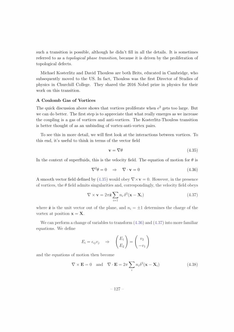
to a 2⇡ shift. A configuration with n = 1 is referred to as a vortex; when n = �1, it is

an anti-vortex. These are examples of topological defects. The configurations of lattice

spins that correspond to a vortex and anti-vortex are shown in the figures.

At the location of the vortex, x = X the field ✓(x) is not well defined. One way to

proceed is to revert to the original XY model and allow the magnitude of to vary

close to the core. However, for our purposes it will su�ce to do something simpler: we

just admit ignorance on short distance scales, and say that the vortex has some core

size which we denote as a. This will later play the role of the UV cut-o↵ in our system.

We’ll start by giving a rough and ready derivation of the e↵ect of vortices. A config-

uration with winding n has r✓ = n

r

(y,�x), and so free energy

Fvortex

=1

2e2

Z

d2x (r✓)2 = ⇡n2

e2log

✓

L

a

◆

+ Fcore

(4.33)

– 125 –

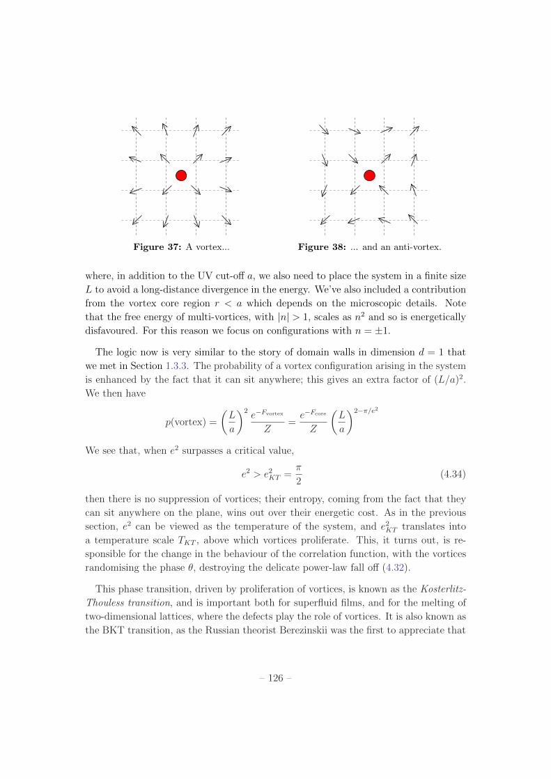
Figure 37: A vortex... Figure 38: ... and an anti-vortex.

where, in addition to the UV cut-o↵ a, we also need to place the system in a finite size

L to avoid a long-distance divergence in the energy. We’ve also included a contribution

from the vortex core region r < a which depends on the microscopic details. Note

that the free energy of multi-vortices, with |n| > 1, scales as n2 and so is energetically

disfavoured. For this reason we focus on configurations with n = ±1.

The logic now is very similar to the story of domain walls in dimension d = 1 that

we met in Section 1.3.3. The probability of a vortex configuration arising in the system

is enhanced by the fact that it can sit anywhere; this gives an extra factor of (L/a)2.

We then have

p(vortex) =

✓

L

a

◆

2 e�Fvortex

Z=

e�Fcore

Z

✓

L

a

◆

2�⇡/e

2

We see that, when e2 surpasses a critical value,

e2 > e2KT

=⇡

2(4.34)

then there is no suppression of vortices; their entropy, coming from the fact that they

can sit anywhere on the plane, wins out over their energetic cost. As in the previous

section, e2 can be viewed as the temperature of the system, and e2KT

translates into

a temperature scale TKT

, above which vortices proliferate. This, it turns out, is re-

sponsible for the change in the behaviour of the correlation function, with the vortices

randomising the phase ✓, destroying the delicate power-law fall o↵ (4.32).

This phase transition, driven by proliferation of vortices, is known as the Kosterlitz-

Thouless transition, and is important both for superfluid films, and for the melting of

two-dimensional lattices, where the defects play the role of vortices. It is also known as

the BKT transition, as the Russian theorist Berezinskii was the first to appreciate that

– 126 –

such a transition is possible, although he didn’t fill in all the details. It is sometimes

referred to as a topological phase transition, because it is driven by the proliferation of

topological defects.

Michael Kosterlitz and David Thouless are both Brits, educated in Cambridge, who

subsequently moved to the US. In fact, Thouless was the first Director of Studies of

physics in Churchill College. They shared the 2016 Nobel prize in physics for their

work on this transition.

A Coulomb Gas of Vortices

The quick discussion above shows that vortices proliferate when e2 gets too large. But

we can do better. The first step is to appreciate that what really emerges as we increase

the coupling is a gas of vortices and anti-vortices. The Kosterlitz-Thouless transition

is better thought of as an unbinding of vortex-anti-vortex pairs.

To see this in more detail, we will first look at the interactions between vortices. To

this end, it’s useful to think in terms of the vector field

v = r✓ (4.35)

In the context of superfluids, this is the velocity field. The equation of motion for ✓ is

r2✓ = 0 ) r · v = 0 (4.36)

A smooth vector field defined by (4.35) would obeyr⇥v = 0. However, in the presence

of vortices, the ✓ field admits singularities and, correspondingly, the velocity field obeys

r⇥ v = 2⇡zX

i=1

ni

�2(x�Xi

) (4.37)

where z is the unit vector out of the plane, and ni

= ±1 determines the charge of the

vortex at position x = X.

We can perform a change of variables to transform (4.36) and (4.37) into more familiar

equations. We define

Ei

= ✏ij

vj

)

E1

E2

!

=

v2

�v1

!

and the equations of motion then become

r⇥ E = 0 and r · E = 2⇡X

i

ni

�2(x�Xi

) (4.38)

– 127 –

These are the Maxwell equations for the auxiliary electric field E, with the vortices

acting as “electric charge”. This means that we can import our machinery from our

course on Electromagnetism; the only di↵erence is that our electric field lives in d = 2

spatial dimensions. For example, to determine the interaction between two vortices,

we need to solve the Gauss’ law equation in (4.38). We do this by writing E = �r�,where

�(x) = �X

i

ni

log

✓

x�Xi

a

◆

(4.39)

The free energy (4.31) can be expressed in terms of the electric field as

F =

Z

d2x1

2e2E · E =

Z

d2x1

2e2(r�)2

This looks very similar to our starting point (4.31), except that the relationship between

the original field ✓(x) and the new field �(x) is given by @i

✓ = ✏ij

@j

�, which is not

straightforward to solve. However, it is now straightforward to compute the free energy.

First integrating by parts, we have

F =

Z

d2x � 1

2e2�r · E =

⇡

e2

X

i 6=j

ni

nj

log

✓ |Xi

�Xj

|a

◆

+X

i

n2

i

Fcore

where, to get the second equality, we’ve substituted in the expressions (4.38) and (4.39)

and, for the cases i = j, replaced our expression with the energy of the core of the

vortex. We learn that the interaction between vortices grows logarithmically. This is

the Coulomb force in d = 2 dimensions; it is repulsive for vortex pairs, and attractive

for a vortex-anti-vortex pair.

We can now use this expression to write down an expression for the partition function

of the XY sigma model. There are two contributions. To isolate these, we decompose

the velocity field as

v = vsw

+ vvortex

The first of these obeys

r⇥ vsw

= 0

This is circulation-free flow in the absence of vortices. It describes the contribution from

the fluctuations of ✓: we call these “spin waves”. The second contribution comes from

– 128 –

vortices and obeys r · vvortex

= 0. The free energy, and hence the partition function,

then factorise into two

Z = Zsw

Zvortex

The spin wave piece is harmless; it shows no sign of a phase transition. Meanwhile, the

vortex piece contains contributions from all number of vortices and anti-vortices. We

restrict attention to configurations that have equal number of vortices and anti-vortices,

as these don’t su↵er the IR divergence (4.33) in their free energy. We’re left with

Zvortex

=1X

p=0

y2p

(p!)2

p

Y

i=1

Z

d2X+

i

d2X�i

exp

⇡

e2

X

i 6=j

ni

nj

log

✓ |Xi

�Xj

|a

◆

!

(4.40)

where y = e�Fcore/a2 can be thought of as the fugacity of vortices. Here X+

i

denote

the positions of p vortices, and X�i

the positions of p anti-vortices. Meanwhile, the

argument of the logarithm involves the sum over the separations Xi

�Xj

, i 6=, j of all

2p (anti)-vortices, regardless of their charge. Finally, the integral should be taken over

all |Xi

�Xj

| > a so that the cores of vortices do not overlap.

Zvortex

is the partition function of a neutral Coulomb gas in the grand canonical

ensemble, with the ± charges interacting through the 2d Coulomb force.

We would like to understand the phase structure of Zvortex

as the coupling e2 is

varied. There are di↵erent ways to go about this. One possibility is to implement the

RG directly on Zvortex

. This proceeds by integrating out the vortices that are separated

on by some short distance scale a, e↵ectively increasing the UV cut-o↵ scale a. Here we

will take an alternative approach. We will first map the Coulomb gas to a seemingly

very di↵erent problem, one which will be more amenable to the traditional RG methods

that we’ve been using in this course.

4.4.2 From Coulomb Gas to Sine-Gordon

The Coulomb gas (4.40) lies in the same universality class as the so-called Sine-Gordon

model. This is a theory of a real scalar field �(x), with free energy,

F =

Z

d2x1

2(r�)2 � � cos(��) (4.41)

The name is a physicist’s version of a joke: it is a play on “Klein-Gordon” theory11.

11Sidney Coleman has a famous paper on this model which starts with the sentence “The Sine-

Gordon equation is the sophomoric but unfortunately standard name for...”.

– 129 –

We start by giving a quick derivation of the equivalence between the Sine-Gordon

model and the Coulomb gas. We will be fairly heuristic. It turns out that this mapping

is somewhat simpler if we revert back to a spatial lattice, rather than working in the

continuum.

To this end, we introduce a lattice with spacing a with lattice sites X↵

. On each

lattice site, we include a variable V↵

which can take values V↵

= �1, 0,+1. The

interpretation is that if V↵

= +1, there is a vortex at this site; if V↵

= �1 there is

an anti-vortex; and if V↵

= 0 the site is empty. We allow V↵

to only take these three

values to reflect the fact that two vortices feel a large repulsion, which means that they

e↵ectively have a hard core, while a vortex and an anti-vortex annihilate to nothing if

they come too close.

The grand canonical partition function (4.40) can then be rewritten as

Zvortex

⇠X

{V↵}exp

⇡

e2

X

↵ 6=�

V↵

V�

log

✓ |X↵

�X�

|a

◆

�X

↵

V 2

↵

Fcore

!

(4.42)

We restrict the sum {V↵

} to configurations that are neutral, soP↵

V↵

= 0. This mimics

the sum over all numbers and positions of vortex-anti-vortex pairs.

To proceed, we will use the fact that the log that appears in Zvortex

is the Green’s

function for the 2d Laplacian r2. In general, we have

Z

D� exp

✓

�Z

d2x1

2(r�)2 + f(x)�(x)

◆

⇠ exp

✓

� 1

4⇡

Z

d2xd2y f(x) log |x� y|f(y)◆

where we’ve dropped a factor of the determinant det(�r2)�1/2 which gives an unim-

portant overall contribution to the partition function. Using this, the partition function

(4.42) can be rewritten yet again as

Zvortex

⇠X

{V↵}

Z

D� exp

�Z

d2x1

2(r�)2 +

X

↵

2⇡i

eV↵

�↵

� V 2

↵

Fcore

!

where we’re using a slightly unholy mix of continuous notation and discrete notation.

You should think of �↵

= �(X↵

) as the value of �(x) at the lattice site, and write your

preferred discretised version of the kinetic term. Now we can do the sum over the V↵

;

– 130 –

we have

Zvortex

=

Z

D� exp

✓

�1

2

Z

d2x (r�)2◆

Y

↵

X

V↵=�1,0,+1

e2⇡ie V↵�↵+V

2↵Fcore

=

Z

D� exp

✓

�1

2

Z

d2x (r�)2◆

Y

↵

h

1 + 2e�Fcore cos(2⇡�↵

/e)i

⇡Z

D� exp✓

�1

2

Z

d2x (r�)2 + 2

a2e�Fcore

Z

d2x cos

✓

2⇡�

e

◆◆

This is the Sine-Gordon model, as promised. Although our derivation used an under-

lying lattice, the final result is expressed as a continuum field theory, and this is the

form we will use moving forward. As always, however, the memory of the lattice will

remain in the UV cut-o↵ scale a. The dictionary between the couplings in (4.41) and

those of the original XY-model are

� =2e�Fcore

a2and � =

2⇡

e

We will now see how these couplings fare under the renormalisation group.

4.4.3 RG Flows in Sine-Gordon

We apply our standard RG programme to the Sine-Gordon model,

F =

Z

d2x1

2(r�)2 � �

0

cos(�0

�)

where we’ve added the subscript 0 to reflect that fact that this free energy is defined

at the cut-o↵ scale ⇤.

What follows next is familiar. We work in Fourier space and decompose the field �

into low and high momentum modes,

�k

= ��k

+ �+

k

where �+

k

includes all modes in the momentum shell ⇤/⇣ < k < ⇤. We also define ��(x)and �+(x) in real space as the inverse Fourier transform of ��

k

and �+

k

respectively.

We then integrate out the high momentum modes to leave ourselves with an e↵ective

free energy,

F 0[��] = F0

[��]� logD

e�FI [��+�

+]

E

+

(4.43)

– 131 –

where

F0

[�] =

Z

d2x1

2(r�)2 and F

I

[�] = ��0

Z

d2x cos(�0

�)

and the expectation value reflects the fact that we’re integrating out the fast momentum

modes, weighted with

he�FI [��+�

+]i+

=

Z

D�+ e�F0[�+] e�FI [�

�+�

+]

Our goal is to compute this e↵ective free energy.

First Order in �0

We will assume that � is suitably small, so that leading order term is⌧

exp

✓

�0

Z

d2x cos�

�(�� + �+)�

◆�

+

⇡ 1 + �0

Z

d2x⌦

cos�

�(�� + �+)�↵

+

= 1 +�0

2

Z

d2xX

�=±1

ei����D

ei���+E

+

Meanwhile, we can use our handy Wick identity (3.34) to writeD

ei���+(x)

E

+

= e��

20/2 h�+

(x)�

+(x)i+

The propagator for the fast mode, evaluated at the same point, is

h�+(0)�+(0)i+

=

Z

⇤

⇤/⇣

d2k

(2⇡)21

k2

=1

2⇡log ⇣ (4.44)

The upshot of this calculation is that the interaction term is renormalised after inte-

grating out the high momentum modes, and becomes

F 0[��] =Z

d2x1

2(r��)2 � �

0

⇣��

2/4⇡ cos(���)

and the coupling �0

becomes

�0 = �0

⇣��

2/4⇡

The next step of the RG is the rescaling, x ! x0 = x/⇣. It’s simple to check that the

rescaling of the field is trivial. With this, our free energy becomes

F 0[�] =Z

d2x1

2(r�)2 � �(⇣) cos(��)

– 132 –

with

�(⇣) = �0

⇣2��

2/4⇡ (4.45)

Already we can see the essence of the Kosterlitz-Thouless phase transition in this

equation. When � is suitably large,

�2 > 8⇡ ) e2 <⇡

2

then the e↵ect of RG is to reduce �. This means that the coupling � cos(��) is an

irrelevant operator and, as we flow towards the infra-red, � ! 0. In this case, the

free energy for � is given just by the gradient terms, and the correlation function will

exhibit a power-law fall o↵.

In contrast, when � is small,

�2 < 8⇡ ) e2 >⇡

2

the operator � cos(��) becomes relevant, growing as we go towards the infra-red12.

Now the minimum of the potential is at � = 0 mod 2⇡/�. Expanding the cos potential

about this minimum gives a quadratic term for � and correlation functions will now

be exponentially suppressed, with a finite correlation length. It is perhaps surprising

that our sophisticated RG analysis gives exactly the same value for the critical coupling

g2

= ⇡/2 as our previous, hand-waving discussion of vortex proliferation (4.34).

Using our earlier result (4.32) for the anomalous dimension, we see that at the phase

transition, e2 = ⇡/2, the system exhibits a universal anomalous dimension,

he�i✓(x) ei✓(0)i ⇠ 1

r1/4

Second Order in �0

At order �20

, we find ourselves with the double cosine

hcos(�(��x

+ �+

x

)) cos(�(��y

+ �+

y

))i+

=1

4

X

�=±1

h

ei��(��x

+�

�y

) hei��(�+x

+�

+y

)i+

+ ei��(��x

��

�y

) hei��(�+x

��

+y

)i+

i

=1

2

h

cos(�(��x

+ ��y

)) e��

2/2h(�+

x

+�

+y

)

2i+

+ cos(�(��x

� ��y

)) e��

2/2h(�+

x

��

+y

)

2i+i

12This same result is derived in a very di↵erent way, using conformal field theory, in the lectures

on String Theory. It can be found in Claim 2 of Section 4.3.3 where, in the notation of that course,

the operator eikX is shown to have dimension � = ↵0k2/2. A quick check of the conventions for the

propagator shows that we should set ↵0 = 1/2⇡ so that � < 2 and the operator is relevant if k2 > 8⇡.

– 133 –

where, as a space-saving measure, I’ve put the spatial position as a subscript, �(x) = �x

.

Taking the logarithm in (4.43) means that we subtract the disconnected diagrams,

hcos(�(��x

+ �+

x

))i2+

. The upshot is that, at order �20

, the e↵ective free energy includes

the piece

F 0[��]�

�

e

2 =�20

4

Z

d2xd2yn

cos(�(��x

+ ��y

))h

e��

2/2h(�+

x

+�

+y

)

2i+ � e��

2/2h�+

x

�

+x

i+e��

2/2h�+

y

�

+y

i+i

+ cos(�(��x

� ��y

))h

e��

2/2h(�+

x

��

+y

)

2i+ � e��

2/2h�+

x

�

+x

i+e��

2/2h�+

y

�

+y

i+io

The expectation values that sit in the exponents are given by

G(x� y; ⇣) = h�+(x)�+(y)i =Z

⇤

⇤/⇣

d2k

(2⇡)2eik·(x�y)

k2

Previously we needed only G(0; ⇣) = 1

2⇡

log ⇣; now we see that the correlator at spatially

separated points also arises. We have

F 0[��]�

�

e

2 =1

4�20

⇣��

2/2⇡

Z

d2xd2yn

cos(�(��x

+ ��y

))h

e��

2G(x�y) � 1

i

+ cos(�(��x

� ��y

))h

e+�

2G(x�y) � 1

io

At first sight, we seem to have a non-local free energy involving a double integral. To

massage it into something more familiar, we need to realise that the function G(r)

receives contributions from a small sliver of Fourier modes, and so decays quickly at

distances r > ⇣/⇤. This means that the functions [e±�G(x�y) � 1] are non-zero only in

a small window |x� y| ⇠ ⇤/⇣.

We write y = x + v and Taylor expand the cos factors in the integral for small v.

For the first, we have simply

cos(�(��x

+ ��y

)) ⇡ cos(2���x

)

The second is more interesting for us; we have

cos(�(��x

� ��y

)) ⇡ 1� �2v2

2(r��)2

Our free energy, at order �20

, then becomes

F 0[��]�

�

e

2 =1

2�20

Z

d2xn

A1

(⇣) cos(2��) + A2

(⇣)(r�)2o

+ const. (4.46)

– 134 –

where all the messy details have been absorbed into two functions

A1

(⇣) =1

2⇣��

2/2⇡

Z

d2vh

e��

2G(v) � 1

i

A2

(⇣) = �1

4⇣��

2/2⇡�2

Z

d2v v2h

e+�

2G(v) � 1

i

(4.47)

We see that the RG flow has generated two terms for us in (4.46). The first, cos(2��),

is something new: it can be thought of the e↵ect of two vortices, which we didn’t

include in our original Sine-Gordon model but is generated upon integrating out high

momentum modes. We will not need this here. The second term is something familiar:

it is renormalisation of our kinetic term. The final steps of the RG procedure tell us

to rescale space, x ! x0 = x/⇣, but also rescale the field � so that the kinetic term

remains canonically normalised, as in (3.6). We have

�0(x0) =q

1 + �20

A2

(⇣)�(x)

This rescaling gets spat out inside the potential, where it has the e↵ect of renormalising

our other coupling, �. We have

�(⇣) = �0

�

1 + �20

A2

(⇣)��1/2 ⇡ �

0

(1� 1

2�20

A2

(⇣)) (4.48)

Recall that, in terms of our original XY model, �2 = 4⇡2/e2. Looking back to our XY

sigma model (4.31), we see renormalises the 1/e2 coe�cient of the kinetic term. This is

sometimes called the spin wave“sti↵ness”, since it measures how di�cult it is to twist

the spins. The intuition behind the result (4.48) is that a gas of vortex-anti-vortex

pairs screens the spins, reducing their sti↵ness.

Beta Functions

Our task now is to understand the global properties of the resulting RG flow. We write

down the beta function in terms of ⇣ = es. From (4.45) we have

d�

ds=

✓

2� �2

4⇡

◆

� =⇣

2� ⇡

e2

⌘

�

Meanwhile, from (4.48), we get

d�

ds= �C(�)�3�2

where C(�) > 0 is a positive function that we could extract from the formula (4.47);

it’s exact value will not be important for us. Written in terms of e2 = 4⇡2/�2, this

– 135 –

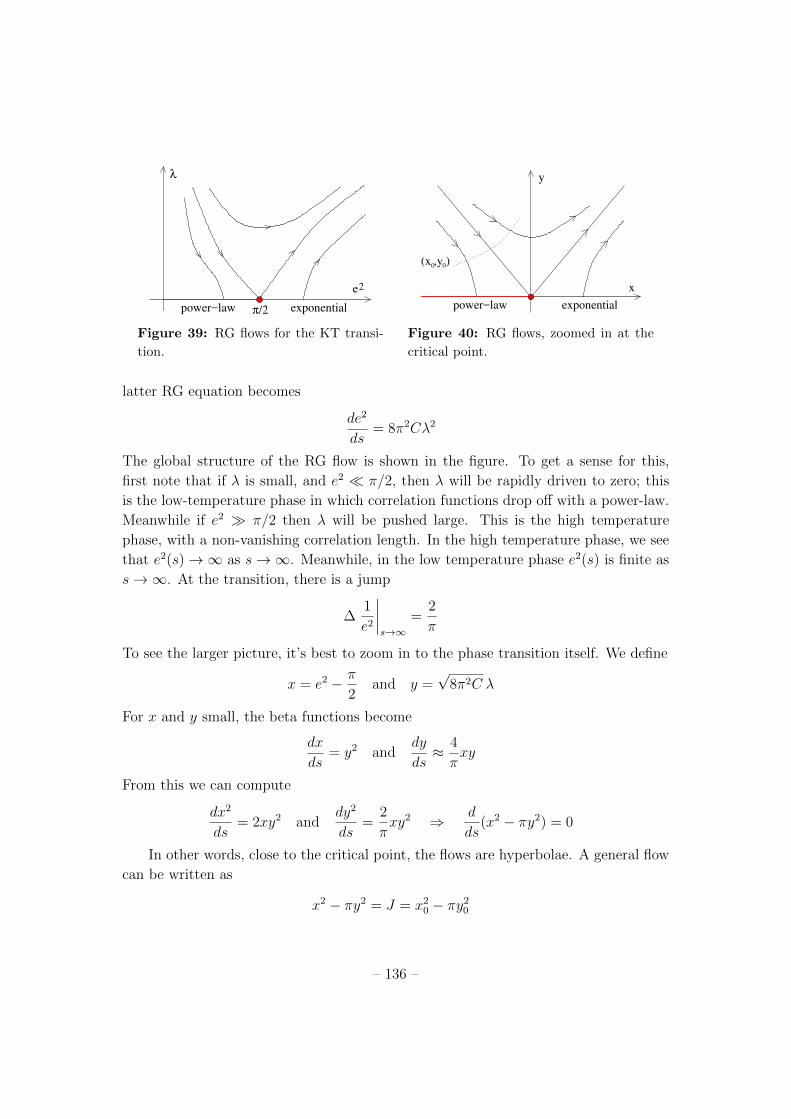
2e

λ

π/2power−law exponential

0(x ,y )0

power−law exponential

x

y

Figure 39: RG flows for the KT transi-

tion.

Figure 40: RG flows, zoomed in at the

critical point.

latter RG equation becomes

de2

ds= 8⇡2C�2

The global structure of the RG flow is shown in the figure. To get a sense for this,

first note that if � is small, and e2 ⌧ ⇡/2, then � will be rapidly driven to zero; this

is the low-temperature phase in which correlation functions drop o↵ with a power-law.

Meanwhile if e2 � ⇡/2 then � will be pushed large. This is the high temperature

phase, with a non-vanishing correlation length. In the high temperature phase, we see

that e2(s) ! 1 as s ! 1. Meanwhile, in the low temperature phase e2(s) is finite as

s ! 1. At the transition, there is a jump

�1

e2

�

�

�

�

s!1=

2

⇡

To see the larger picture, it’s best to zoom in to the phase transition itself. We define

x = e2 � ⇡

2and y =

p8⇡2C �

For x and y small, the beta functions become

dx

ds= y2 and

dy

ds⇡ 4

⇡xy

From this we can compute

dx2

ds= 2xy2 and

dy2

ds=

2

⇡xy2 ) d

ds(x2 � ⇡y2) = 0

In other words, close to the critical point, the flows are hyperbolae. A general flow

can be written as

x2 � ⇡y2 = J = x2

0

� ⇡y20

– 136 –

where (x0

, y0

) are the initial “bare” values of the couplings at the cut-o↵ scale. There

are two regions with J > 0; these correspond to the low and high temperature regimes

that we discussed above. The separatrix at J = 0 is given by x = ±p⇡y. The line

with x = �p⇡y flows directly to the critical point. The line with x = +

p⇡y flows

away from the critical point.

Suppose that we start on the left of the figure, with x < 0. Then the initial data,

shown as a dotted line in the figure, is (x0

, y0

). As we vary this data, we pass through

the phase transition. In this sense, it is natural to think of this initial data as a function

of the temperature (x0

(T ), y0

(T )), with

J(T ) ⇠ Tc

� T

ensuring that we hit the critical point when J = 0¿

Finally, we can ask about the correlation length ⇠. To compute this, we can look at

flows with J < 0 which don’t quite hit the y = 0 axis. We have

dx

ds= y2 =

1

⇡(x2 � J) =

1

⇡(x2 + |J |)

which we can solve to give

s =⇡

p|J |

"

tan�1

xp|J |

!

� tan�1

x0

p|J |

!#

This has the slightly odd property that x ! 1 as s remains finite. This is an artefact

of our approximation but, nonetheless, can be used to our advantage. By the time

x ⇡ 1, we also have y ⇡ 1 and the theory is in the gapped phase. We can stop the RG

flow here and use this as a proxy for our correlation length which, as we approach the

phase transition from above, scales as

⇠ ⇠ aes ⇠ exp

1p|J |

!

⇠ exp

✓

1pT � T

c

◆

We’re are used to a fairly soft divergence in the correlation length as we approach

the critical temperature. For the Kosterlitz-Thouless transition, the change is much

more dramatic. This also has an e↵ect on the thermodynamic free energy which, as

an extensive quantity scales as F ⇠ (L/⇠)2. As we approach the phase transition from

above, we have

Fthermo

⇠ 1

⇠2⇠ exp

✓

� 1pT � T

c

◆

– 137 –

This is a very weak singularity. There is no discontinuity in the heat capacity. Moreover,

there is no discontinuity in any derivative of the free energy. In terms of Ehrenfest’s

original classification, the Kosterlitz-Thouless transition is rather strange: it is a phase

transition of infinite order.

– 138 –