Embed Size (px)
Citation preview

4 1-D Boundary Value Problems Heat Equation
The main purpose of this chapter is to study boundary value problems for the heat equationon a finite rod a ≤ x ≤ b.
ut(x, t) = kuxx(x, t), a < x < b, t > 0
u(x, 0) = ϕ(x)
The main new ingredient is that physical constraints called boundary conditions must beimposed at the ends of the rod. The two main conditions are
u(a, t) = 0, u(b, t) = 0 Dirichlet Conditions
ux(a, t) = 0, ux(b, t) = 0 Neumann Conditions
We can also have any combination of these conditions, i.e., we could have a Dirichlet conditionat x = a and Neumann condition at x = b.
The is one additional important boundary condition
ux(a, t)− k0u(a, t) = 0, ux(b, t) + k1u(b, t) = 0 Robin Conditions
Finally we will a more general problem involving two extra terms that correspond to heatconduction and convection.
ut(x, t) = k(uxx(x, t)− 2au(x, t)x + bu(x, t)
), 0 < x < `, t > 0
u(x, 0) = ϕ(x).
The basic methodology presented here is the idea of eigenvalues and eigenvector expansionsas presented in a linear algebra or differential equations class when studying linear systemsof ODEs. The basic idea can be described by an example. Let X be an n-vector valuedfunction and A an n × n matrix. Also let X0 denote a constant initial condition n-vector.Then to solve the initial value problem
d
dtX = AX, X(0) = X0
we find the eigenvalues {λj}nj=1 and eigenvectors {Φj}nj=1 of A (i.e. AΦj = λjΦj) where wealso assume
〈Φj,Φk〉 = Φ>Φk = δjk ≡
{1 j = k
0 j 6= k.
Then, assuming there are n linearly independent eigenvectors, the solution can be written
X(t) =n∑j=1
eλjt〈X0,Φj〉Φj.
The generalization of this idea to the one dimensional heat equation involves the generalizedtheory of Fourier series. This method due to Fourier was develop to solve the heat equationand it is one of the most successful ideas in mathematics. We will begin our study withclassical Fourier series and then turn to the heat equation and Fourier’s idea of separationof variables.
1

4.1 Fourier Series
A series of the functions
φ0 =1
2, φ(1)
n = cos(nx), φ(2)n = sin(nx), for n ≥ 1
written in a series1
2a0 +
∞∑n=1
(an cos(nx) + bn sin(nx)
)is known as a Fourier series. (We choose φ0 = 1
2so all of the functions have the same norm.)
A fairly general class of functions can be expanded in Fourier series. Let f(x) be a functiondefined on −π < x < π. Assume that f(x) can be expanded in a Fourier series
f(x) ∼ 1
2a0 +
∞∑n=1
(an cos(nx) + bn sin(nx)
). (4.1)
Here the “∼” means “has the Fourier series”. We have not said if the series converges yet.For now let’s assume that the series converges uniformly so we can replace the ∼ with an =.
We integrate Equation 4.1 from −π to π to determine a0.∫ π
−πf(x) dx =
1
2a0
∫ π
−πdx+
∫ π
−π
∞∑n=1
an cos(nx) + bn sin(nx) dx
= πa0 +∞∑n=1
(an
∫ π
−πcos(nx) dx+ bn
∫ π
−πsin(nx) dx
)= πa0
So that
a0 =1
π
∫ π
−πf(x) dx.
Multiplying by cos(mx) and integrating will enable us to solve for am.∫ π
−πf(x) cos(mx) dx =
1
2a0
∫ π
−πcos(mx) dx
+∞∑n=1
(an
∫ π
−πcos(nx) cos(mx) dx+ bn
∫ π
−πsin(nx) cos(mx) dx
)All but one of the terms on the right side vanishes due to the orthogonality of the functions.∫ π
−πf(x) cos(mx) dx = am
∫ π
−πcos(mx) cos(mx) dx
= am
∫ π
−π
1
2(1 + cos(2mx)) dx
= πam
2

So that
am =1
π
∫ π
−πf(x) cos(mx) dx m = 0, 1, 2, . . .
Similarly, we can multiply by sin(mx) and integrate to solve for bm. The result is
bm =1
π
∫ π
−πf(x) sin(mx) dx m = 1, 2, 3, . . . .
an and bn are called Fourier coefficients.
Although we will not show it, Fourier series converge for a fairly general class of functions.Let f(x−) denote the left limit of f(x) and f(x+) denote the right limit.
Example 4.1. For the function defined
f(x) =
{0 for x < 0,
x+ 1 for x ≥ 0,
the left and right limits at x = 0 are
f(0−) = 0, f(0+) = 1.
Theorem 4.1. Let f(x) be a 2π-periodic function for which∫ π−π |f(x)| dx exists. Define the
Fourier coefficients
an =1
π
∫ π
−πf(x) cos(nx) dx, bn =
1
π
∫ π
−πf(x) sin(nx) dx.
If x is an interior point of an interval on which f(x) has limited total fluctuation, then theFourier series of f(x)
a0
2+∞∑n=1
(an cos(nx) + bn sin(nx)
),
converges to 12(f(x−) + f(x+)). If f is continuous at x, then the series converges to f(x).
Example 4.2. Consider the function defined by
f(x) =
{−x for − π ≤ x < 0
π − 2x for 0 ≤ x < π.
The Fourier series converges to the function defined by
f̂(x) =
0 for x = −π−x for − π < x < 0
π/2 for x = 0
π − 2x for 0 < x < π.
The function f̂(x) is plotted in the following figure.
3
-3 -2 -1 1 2 3
-3
-2
-1
1
2
3
Figure 1: Graph of f̂(x).
A lot can be learned about the Fourier coefficients from the geometry of the function. Forexample, if f(x) is an even function, (f(−x) = f(x)), then there will not be any sine termsin the Fourier series for f(x). The Fourier sine coefficient is
bn =1
π
∫ π
−πf(x) sin(nx) dx.
Since f(x) is an even function and sin(nx) is odd, f(x) sin(nx) is odd. bn is the integral ofan odd function from −π to π and is thus zero. Also we can simplify the cosine coefficients,
an =1
π
∫ π
−πf(x) cos(nx) dx
=2
π
∫ π
0
f(x) cos(nx) dx.
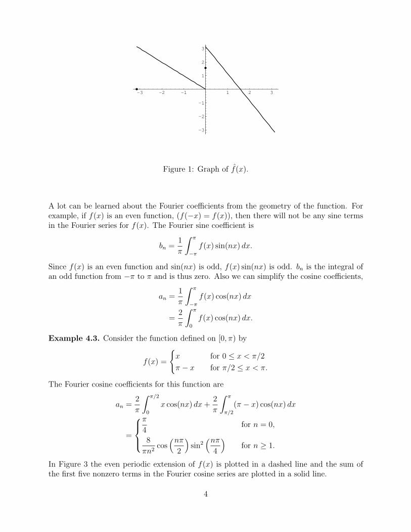
Example 4.3. Consider the function defined on [0, π) by
f(x) =
{x for 0 ≤ x < π/2
π − x for π/2 ≤ x < π.
The Fourier cosine coefficients for this function are
an =2
π
∫ π/2
0
x cos(nx) dx+2
π
∫ π
π/2
(π − x) cos(nx) dx
=
π
4for n = 0,
8
πn2cos(nπ
2
)sin2
(nπ4
)for n ≥ 1.
In Figure 3 the even periodic extension of f(x) is plotted in a dashed line and the sum ofthe first five nonzero terms in the Fourier cosine series are plotted in a solid line.
4

-3 -2 -1 1 2 3
0.25
0.5
0.75
1
1.25
1.5
Figure 3: Fourier Cosine Series.
If, on the other hand, f(x) is an odd function, (f(−x) = −f(x)), then there will not beany cosine terms in the Fourier series. Since f(x) cos(nx) is an odd function, the cosinecoefficients will be zero. Since f(x) sin(nx) is an even function,we can rewrite the sinecoefficients
bn =2
π
∫ π
0
f(x) sin(nx) dx.
Example 4.4. Consider the function defined on [0, π) by
f(x) =
{x for 0 ≤ x < π/2
π − x for π/2 ≤ x < π.
The Fourier sine coefficients for this function are
bn =2
π
∫ π/2
0
x sin(nx) dx+2
π
∫ π
π/2
(π − x) sin(nx) dx
=16
πn2cos(nπ
4
)sin3
(nπ4
)In Figure 4 the odd periodic extension of f(x) is plotted in a dashed line and the sum of thefirst five nonzero terms in the Fourier sine series are plotted in a solid line.
-3 -2 -1 1 2 3
-1.5
-1
-0.5
0.5
1
1.5
Figure 4: Fourier Sine Series.
5

4.2 Fourier series for arbitrary interval
The above formulas can easily be extended to periodic functions with an arbitrary period2` defined on [−`, `] and, using even and odd extensions, we can even write Fourier seriesexpansions for functions defined on an interval [0, `]. We present these formulas below.
1. For f(x) = f(x+ 2`) and f is piecewise smooth on −` ≤ x ≤ `. Then for all x ∈ R
f(x+) + f(x−)
2= a0 +
∞∑n=1
{an cos
(nπx`
)+ bn sin
(nπx`
)},
where
a0 =1
2`
∫ `
−`f(x) dx,
an =1
`
∫ `
−`f(x) cos
(nπx`
)dx
bn =1
`
∫ `
−`f(x) sin
(nπx`
)dx.
If f is continuous (at x) then
f(x+) + f(x−)
2= f(x).
2. Fourier Cosine: Given f on [0, `]
a0 =1
`
∫ `
0
f(x) dx, an =2
`
∫ `
0
f(x) cos(nπx
`
)dx
f(x+) + f(x−)
2= a0 +
∞∑n=1
an cos(nπx
`
)3. Fourier Sine: Given f on [0, `]
bn =2
`
∫ `
0
f(x) sin(nπx
`
)dx
f(x+) + f(x−)
2=∞∑n=1
bn sin(nπx
`
)
6

4.3 Heat Equation Dirichlet Boundary Conditions
ut(x, t) = kuxx(x, t), 0 < x < `, t > 0 (4.2)
u(0, t) = 0, u(`, t) = 0
u(x, 0) = ϕ(x)
1. Separate Variables Look for simple solutions in the form
u(x, t) = ϕ(x)ψ(t).
Substituting into (4.14) and dividing both sides by ϕ(x)ψ(t) gives
ψ̇(t)
kψ(t)=ϕ′′(x)
ϕ(x)
Since the left side is independent of x and the right side is independent of t, it followsthat the expression must be a constant:
ψ̇(t)
kψ(t)=ϕ′′(x)
ϕ(x)= λ.
(Here ψ̇ means the derivative of ψ with respect to t and ϕ′ means means the derivativeof ϕ with respect to x.) We seek to find all possible constants λ and the correspondingnonzero functions ϕ and ψ.
We obtainϕ′′ − λϕ = 0, ψ̇ − kλψ = 0.
The solution of the second equation is
ψ(t) = Cekλt (4.3)
where C is an arbitrary constant. Furthermore, the boundary conditions give
ϕ(0)ψ(t) = 0, ϕ(`)ψ(t) = 0 for all t.
Since ψ(t) is not identically zero we obtain the desired eigenvalue problem
ϕ′′(x)− λϕ(x) = 0, ϕ(0) = 0, ϕ(`) = 0. (4.4)
2. Find Eigenvalues and Eignevectors The next main step is to find the eigenvaluesand eigenfunctions from (4.16). There are, in general, three cases:
(a) If λ = 0 then ϕ(x) = ax+ b so applying the boundary conditions we get
0 = ϕ(0) = b, 0 = ϕ(`) = a` ⇒ a = b = 0.
Zero is not an eigenvalue.
7

(b) If λ = µ2 > 0 thenϕ(x) = a cosh(µx) + b sinh(µx).
Applying the boundary conditions we have
0 = ϕ(0) = a⇒ a = 0 0 = ϕ(`) = b sinh(µ`) ⇒ b = 0.
Therefore, there are no positive eigenvalues.
Consider the following alternative argument: If ϕ′′(x) = λϕ(x) then multiplyingby ϕ we have ϕ(x)ϕ′′(x) = λϕ(x)2. Integrate this expression from x = 0 to x = `.We have
λ
∫ `
0
ϕ(x)2 dx =
∫ `
0
ϕ(x)ϕ′′(x) dx = −∫ `
0
ϕ′(x)2 dx+ ϕ(x)ϕ′(x)
∣∣∣∣`0
.
Since ϕ(0) = ϕ(`) = 0 we conclude
λ = −
∫ `
0
ϕ′(x)2 dx∫ `
0
ϕ(x)2 dx
and we see that λ must be less than or equal to zero.
(c) So, finally, consider λ = −µ2 so that
ϕ(x) = a cos(µx) + b sin(µx).
Applying the boundary conditions we have
0 = ϕ(0) = a⇒ a = 0 0 = ϕ(`) = b sin(µ`).
From this we conclude sin(µ`) = 0 which implies
µ =nπ
`
and therefore
λn = −µ2n = −
(nπ`
)2
, ϕn(x) = bn sin(µnx), n = 1, 2, · · · .. (4.5)
From (4.15) we also have the associated functions ψn(t) = ekλnt.
3. Write Formal Sum From the above considerations we can conclude that for anyinteger N and constants {bn}Nn=0
uN(x, t) =N∑n=1
bnψn(t)ϕn(x) =N∑n=1
bnekλnt sin
(nπx`
).
satisfies the differential equation in (4.14) and the boundary conditions.
8
4. Use Fourier Series to Find Coefficients The only problem remaining is to somehowpick the constants bn so that the initial condition u(x, 0) = ϕ(x) is satisfied. To dothis we consider what we learned from Fourier series. In particular we look for u as aninfinite sum
u(x, t) =∞∑n=1
bnekλnt sin
(nπx`
)and we try to find {bn} satisfying
ϕ(x) = u(x, 0) =∞∑n=1
bn sin(nπx
`
).
But this nothing more than a Sine expansion of the function ϕ on the interval (0, `).
bn =2
`
∫ `
0
ϕ(x) sin(nπx
`
)dx. (4.6)
Example 4.5. As an explicit example for the initial condition consider ` = 1, k = 1/10 and
ϕ(x) = x(1− x). Let us recall that µn =(nπ`
)which in this case reduces to nπ.
bn = 2
∫ 1
0
x(1− x) sin (nπx) dx
= 2
∫ 1
0
x(1− x)
(−cos (nπx)
nπ
)′dx
=2
nπ
[−x(1− x)
cos(nπx)
nπ
∣∣∣∣10
+
∫ 1
0
(1− 2x)cos(nπx)
µndx
]
=2
nπ
∫ 1
0
(1− 2x)
(sin (nπx)
nπ
)′dx
=2
nπ
[(1− 2x)
sin(nπx)
nπ
∣∣∣∣10
−∫ 1
0
(−2)sin (nπx)
nπdx
]
=4
(nπ)2
∫ 1
0
sin(nπx) dx =4
(nπ)2
[−cos(nπx)
nπ
∣∣∣∣10
]=
4 [1− (−1)n]
(nπ)3
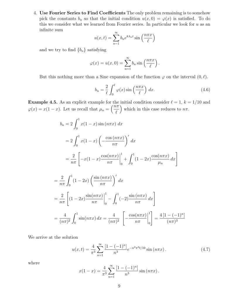
We arrive at the solution
u(x, t) =4
π3
∞∑n=1
[1− (−1)n]
n3e−n
2π2t/10 sin (nπx) . (4.7)
where
x(1− x) =4
π3
∞∑n=1
[1− (−1)n]
n3sin (nπx) .
9

As an example with N = 3 we have
x(1− x) ≈ 8
π3
(sin(πx) +
sin(3πx)
27
).
In the following figure we plot the left and right hand side of the above.
x0 0.2 0.4 0.6 0.8 1.0
0
0.05
0.10
0.15
0.20
0.25
Finally we plot the approximate solution at times t = 0, t =, t = 2, t = 3
u(x, t) =4
π3
3∑n=1
[1− (−1)n]
n3e−n
2π2t/10 sin (nπx) .
x0 0.2 0.4 0.6 0.8 1.0
0
0.05
0.10
0.15
0.20
4.4 Heat Equation Neumann Boundary Conditions
ut(x, t) = uxx(x, t), 0 < x < `, t > 0 (4.8)
ux(0, t) = 0, ux(`, t) = 0
u(x, 0) = ϕ(x)
10
1. Separate Variables Look for simple solutions in the form
u(x, t) = ϕ(x)ψ(t).
Substituting into (4.8) and dividing both sides by ϕ(x)ψ(t) gives
ψ̇(t)
ψ(t)=ϕ′′(x)
ϕ(x)
Since the left side is independent of x and the right side is independent of t, it followsthat the expression must be a constant:
ψ̇(t)
ψ(t)=ϕ′′(x)
ϕ(x)= λ.
(Here ψ̇ means the derivative of ψ with respect to t and ϕ′ means means the derivativeof ϕ with respect to x.) We seek to find all possible constants λ and the correspondingnonzero functions ϕ and ψ.
We obtainϕ′′ − λϕ = 0, ψ̇ − λψ = 0.
The solution of the second equation is
ψ(t) = Ceλt (4.9)
where C is an arbitrary constant. Furthermore, the boundary conditions give
ϕ′(0)ψ(t) = 0, ϕ′(`)ψ(t) = 0 for all t.
Since ψ(t) is not identically zero we obtain the desired eigenvalue problem
ϕ′′(x)− λϕ(x) = 0, ϕ′(0) = 0, ϕ′(`) = 0. (4.10)
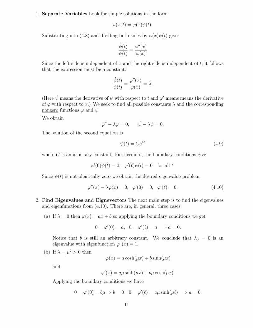
2. Find Eigenvalues and Eignevectors The next main step is to find the eigenvaluesand eigenfunctions from (4.10). There are, in general, three cases:
(a) If λ = 0 then ϕ(x) = ax+ b so applying the boundary conditions we get
0 = ϕ′(0) = a, 0 = ϕ′(`) = a ⇒ a = 0.
Notice that b is still an arbitrary constant. We conclude that λ0 = 0 is aneigenvalue with eigenfunction ϕ0(x) = 1.
(b) If λ = µ2 > 0 thenϕ(x) = a cosh(µx) + b sinh(µx)
andϕ′(x) = aµ sinh(µx) + bµ cosh(µx).
Applying the boundary conditions we have
0 = ϕ′(0) = bµ⇒ b = 0 0 = ϕ′(`) = aµ sinh(µ`) ⇒ a = 0.
11

Therefore, there are no positive eigenvalues.
Consider the following alternative argument: If ϕ′′(x) = λϕ(x) then multiplyingby ϕ we have ϕ(x)ϕ′′(x) = λϕ(x)2. Integrate this expression from x = 0 to x = `.We have
λ
∫ `
0
ϕ(x)2 dx =
∫ `
0
ϕ(x)ϕ′′(x) dx = −∫ `
0
ϕ′(x)2 dx+ ϕ(x)ϕ′(x)
∣∣∣∣`0
.
Since ϕ′(0) = ϕ′(`) = 0 we conclude
λ = −
∫ `
0
ϕ′(x)2 dx∫ `
0
ϕ(x)2 dx
and we see that λ must be less than or equal to zero ( zero only if ϕ′ = 0).
(c) So, finally, consider λ = −µ2 so that
ϕ(x) = a cos(µx) + b sin(µx)
andϕ′(x) = −aµ sin(µx) + bµ cos(µx).
Applying the boundary conditions we have
0 = ϕ′(0) = bµ⇒ b = 0 0 = ϕ′(`) = −aµ sin(µ`).
From this we conclude sin(µ`) = 0 which implies µ =nπ
`and therefore
λn = −µ2n = −
(nπ`
)2
, ϕn(x) = cos(µnx), n = 1, 2, · · · .. (4.11)
From (4.9) we also have the associated functions ψn(t) = eλnt.
3. Write Formal Infinite Sum From the above considerations we can conclude thatfor any integer N and constants {an}Nn=0
un(x, t) =a0
2+
N∑n=1
anψn(t)ϕn(x) = a0 +N∑n=1
aneλnt cos
(nπx`
).
satisfies the differential equation in (4.8) and the boundary conditions.
4. Use Fourier Series to Find Coefficients The only problem remaining is to somehowpick the constants an so that the initial condition u(x, 0) = ϕ(x) is satisfied. To dothis we consider what we learned from Fourier series. In particular we look for u as aninfinite sum
u(x, t) = a0 +∞∑n=1
aneλnt cos
(nπx`
)
12

and we try to find {an} satisfying
ϕ(x) = u(x, 0) = a0 +∞∑n=1
an cos(nπx
`
).
But this nothing more than a Cosine expansion of the function ϕ on the interval (0, `).
Our work on Fourier series showed us that
a0 =2
`
∫ `
0
ϕ(x) dx, an =2
`
∫ `
0
ϕ(x) cos(nπx
`
)dx. (4.12)
As an explicit example for the initial condition consider ` = 1 and ϕ(x) = x(1− x). In thiscase (4.12) becomes
a0 = 2
∫ 1
0
ϕ(x) dx, an = 2
∫ 1
0
ϕ(x) cos (nπx) dx.
We have
a0 = 2
∫ 1
0
ϕ(x) dx = 2
∫ 1
0
x(1− x) dx
= 2
[x2
2− x3
3
] ∣∣∣∣10
=1
3.
and
an = 2
∫ 1
0
ϕ(x) cos (nπx) dx = 2
∫ 1
0
x(1− x) cos (nπx) dx
= 2
∫ 1
0
x(1− x)
(sin (nπx)
nπ
)′dx
= 2
[x(1− x)
sin (nπx)
nπ
∣∣∣∣10
−∫ 1
0
(1− 2x)sin (nπx)
nπdx
]
=2
nπ
∫ 1
0
(1− 2x)
(cos (nπx)
nπ
)′dx
=2
nπ
[(1− 2x)
cos (nπx)
nπ
∣∣∣∣10
−∫ 1
0
(−2)cos (nπx)
nπdx
]
=2
nπ
[−cos (nπ)
nπ− 1
nπ
]
=−2
(nπ)2((−1)n + 1) =
−4
(nπ)2, n even
0, n odd
.
13
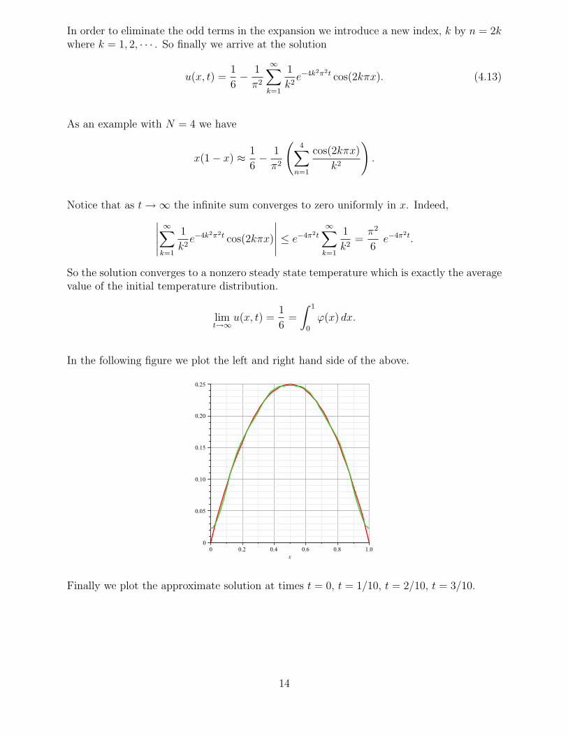
In order to eliminate the odd terms in the expansion we introduce a new index, k by n = 2kwhere k = 1, 2, · · · . So finally we arrive at the solution
u(x, t) =1
6− 1
π2
∞∑k=1
1
k2e−4k2π2t cos(2kπx). (4.13)
As an example with N = 4 we have
x(1− x) ≈ 1
6− 1
π2
(4∑
n=1
cos(2kπx)
k2
).
Notice that as t→∞ the infinite sum converges to zero uniformly in x. Indeed,∣∣∣∣∣∞∑k=1
1
k2e−4k2π2t cos(2kπx)
∣∣∣∣∣ ≤ e−4π2t
∞∑k=1
1
k2=π2
6e−4π2t.
So the solution converges to a nonzero steady state temperature which is exactly the averagevalue of the initial temperature distribution.
limt→∞
u(x, t) =1
6=
∫ 1
0
ϕ(x) dx.
In the following figure we plot the left and right hand side of the above.
x0 0.2 0.4 0.6 0.8 1.0
0
0.05
0.10
0.15
0.20
0.25
Finally we plot the approximate solution at times t = 0, t = 1/10, t = 2/10, t = 3/10.
14

x0.0 0.2 0.4 0.6 0.8 1.0
0.05
0.10
0.15
0.20
4.5 Heat Equation Dirichlet-Neumann Boundary Conditions
ut(x, t) = uxx(x, t), 0 < x < `, t > 0 (4.14)
u(0, t) = 0, ux(`, t) = 0
u(x, 0) = ϕ(x)
1. Separate Variables Look for simple solutions in the form
u(x, t) = ϕ(x)ψ(t).
Substituting into (4.14) and dividing both sides by ϕ(x)ψ(t) gives
ψ̇(t)
ψ(t)=ϕ′′(x)
ϕ(x)
Since the left side is independent of x and the right side is independent of t, it followsthat the expression must be a constant:
ψ̇(t)
ψ(t)=ϕ′′(x)
ϕ(x)= λ.
(Here ψ̇ means the derivative of ψ with respect to t and ϕ′ means means the derivativeof ϕ with respect to x.) We seek to find all possible constants λ and the correspondingnonzero functions ϕ and ψ.
We obtainϕ′′ − λϕ = 0, ψ̇ − λψ = 0.
The solution of the second equation is
ψ(t) = Ceλt (4.15)
15

where C is an arbitrary constant. Furthermore, the boundary conditions give
ϕ(0)ψ(t) = 0, ϕ′(`)ψ(t) = 0 for all t.
Since ψ(t) is not identically zero we obtain the desired eigenvalue problem
ϕ′′(x)− λϕ(x) = 0, ϕ(0) = 0, ϕ′(`) = 0. (4.16)
2. Find Eigenvalues and Eignevectors The next main step is to find the eigenvaluesand eigenfunctions from (4.16). There are, in general, three cases:
(a) If λ = 0 then ϕ(x) = ax+ b so applying the boundary conditions we get
0 = ϕ(0) = b, 0 = ϕ′(`) = a ⇒ a = b = 0.
Zero is not an eigenvalue.
(b) If λ = µ2 > 0 thenϕ(x) = a cosh(µx) + b sinh(µx)
andϕ′(x) = aµ sinh(µx) + bµ cosh(µx).
Applying the boundary conditions we have
0 = ϕ′(0) = aµ⇒ a = 0 0 = ϕ′(`) = bµ cosh(µ`) ⇒ b = 0.
Therefore, there are no positive eigenvalues.
Consider the following alternative argument: If ϕ′′(x) = λϕ(x) then multiplyingby ϕ we have ϕ(x)ϕ′′(x) = λϕ(x)2. Integrate this expression from x = 0 to x = `.We have
λ
∫ `
0
ϕ(x)2 dx =
∫ `
0
ϕ(x)ϕ′′(x) dx = −∫ `
0
ϕ′(x)2 dx+ ϕ(x)ϕ′(x)
∣∣∣∣`0
.
Since ϕ(0) = ϕ′(`) = 0 we conclude
λ = −∫ `
0ϕ′(x)2 dx∫ `
0ϕ(x)2 dx
and we see that λ must be less than or equal to zero.
(c) So, finally, consider λ = −µ2 so that
ϕ(x) = a cos(µx) + b sin(µx)
andϕ′(x) = −aµ sin(µx) + bµ cos(µx).
Applying the boundary conditions we have
0 = ϕ(0) = aµ⇒ a = 0 0 = ϕ′(`) = bµ cos(µ`).
16
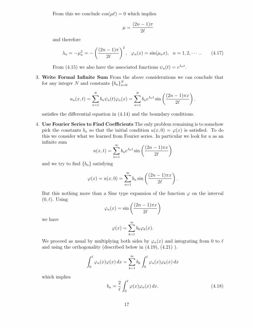
From this we conclude cos(µ`) = 0 which implies
µ =(2n− 1)π
2`
and therefore
λn = −µ2n = −
((2n− 1)π
2`
)2
, ϕn(x) = sin(µnx), n = 1, 2, · · · .. (4.17)
From (4.15) we also have the associated functions ψn(t) = eλnt.
3. Write Formal Infinite Sum From the above considerations we can conclude thatfor any integer N and constants {bn}Nn=0
un(x, t) =N∑n=1
bnψn(t)ϕn(x) =N∑n=1
bneλnt sin
((2n− 1)πx
2`
).
satisfies the differential equation in (4.14) and the boundary conditions.
4. Use Fourier Series to Find Coefficients The only problem remaining is to somehowpick the constants bn so that the initial condition u(x, 0) = ϕ(x) is satisfied. To dothis we consider what we learned from Fourier series. In particular we look for u as aninfinite sum
u(x, t) =∞∑n=1
bneλnt sin
((2n− 1)πx
2`
)and we try to find {bn} satisfying
ϕ(x) = u(x, 0) =∞∑n=1
bn sin
((2n− 1)πx
2`
).
But this nothing more than a Sine type expansion of the function ϕ on the interval(0, `). Using
ϕn(x) = sin
((2n− 1)πx
2`
)we have
ϕ(x) =∞∑k=1
bkϕk(x).
We proceed as usual by multiplying both sides by ϕn(x) and integrating from 0 to `and using the orthogonality (described below in (4.19), (4.21) ).∫ `
0
ϕn(x)ϕ(x) dx =∞∑k=1
bk
∫ `
0
ϕn(x)ϕk(x) dx
which implies
bn =2
`
∫ `
0
ϕ(x)ϕn(x) dx. (4.18)
17

Orthogonality: ∫ `
0
ϕn(x)ϕk(x) dx =
`
2, n = k
0, n 6= k
.
To see this recall that ϕ′′j = λjϕj and ϕj(0) = 0, ϕ′j(`) = 0. First consider n 6= k soλn 6= λk and therefore
λn
∫ `
0
ϕn(x)ϕk(x) dx =
∫ `
0
ϕ′′n(x)ϕk(x) dx (4.19)
= −∫ `
0
ϕ′n(x)ϕ′k(x) dx+ [ϕ′n(x)ϕk(x)]
∣∣∣∣`0
=
∫ `
0
ϕn(x)ϕ′′k(x) dx+ [ϕ′n(x)ϕk(x)− ϕn(x)ϕ′k(x)]
∣∣∣∣`0
= λk
∫ `
0
ϕn(x)ϕk(x) dx. (4.20)
Therefore
(λn − λk)∫ `
0
ϕn(x)ϕk(x) dx = 0 ⇒∫ `
0
ϕn(x)ϕk(x) dx = 0.
For n = k we have∫ `
0
ϕ2n(x) dx =
∫ `
0
sin2
((2n− 1)πx
2`
)dx (4.21)
=1
2
∫ `
0
(1− cos
((2n− 1)πx
`
))dx
=`
2− 1
2
(`
(2n− 1)π
)sin
((2n− 1)πx
`
) ∣∣∣∣`0
=`
2. (4.22)
As an explicit example for the initial condition consider ϕ(x) = x. Let us recall that
µn =
((2n− 1)π
2`
)
18
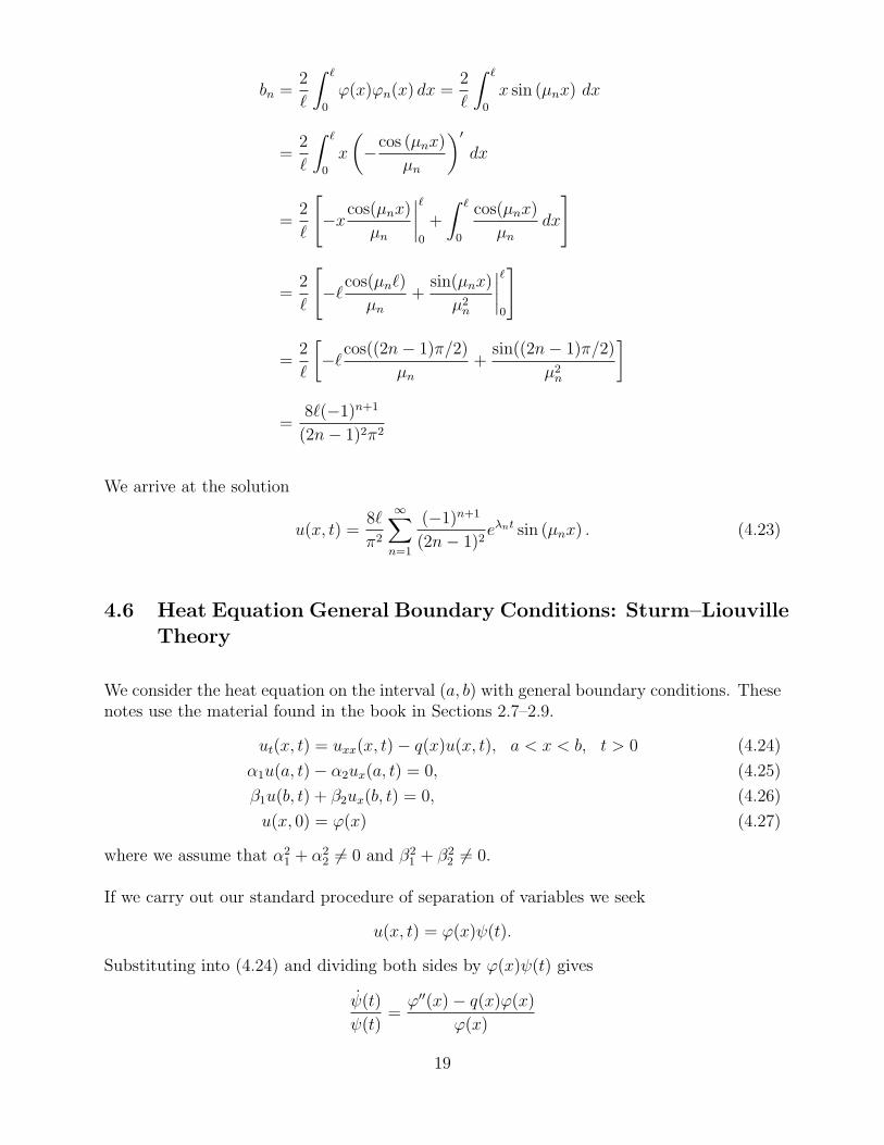
bn =2
`
∫ `
0
ϕ(x)ϕn(x) dx =2
`
∫ `
0
x sin (µnx) dx
=2
`
∫ `
0
x
(−cos (µnx)
µn
)′dx
=2
`
[−xcos(µnx)
µn
∣∣∣∣`0
+
∫ `
0
cos(µnx)
µndx
]
=2
`
[−`cos(µn`)
µn+
sin(µnx)
µ2n
∣∣∣∣`0
]
=2
`
[−`cos((2n− 1)π/2)
µn+
sin((2n− 1)π/2)
µ2n
]
=8`(−1)n+1
(2n− 1)2π2
We arrive at the solution
u(x, t) =8`
π2
∞∑n=1
(−1)n+1
(2n− 1)2eλnt sin (µnx) . (4.23)
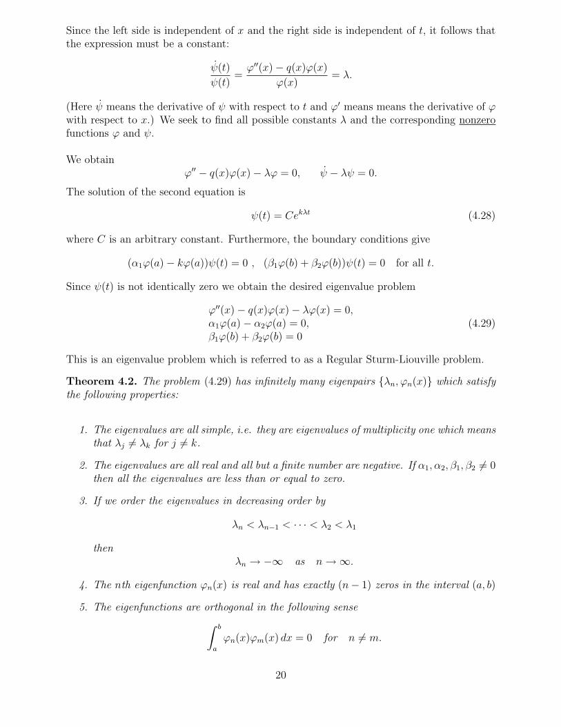
4.6 Heat Equation General Boundary Conditions: Sturm–LiouvilleTheory
We consider the heat equation on the interval (a, b) with general boundary conditions. Thesenotes use the material found in the book in Sections 2.7–2.9.
ut(x, t) = uxx(x, t)− q(x)u(x, t), a < x < b, t > 0 (4.24)
α1u(a, t)− α2ux(a, t) = 0, (4.25)
β1u(b, t) + β2ux(b, t) = 0, (4.26)
u(x, 0) = ϕ(x) (4.27)
where we assume that α21 + α2
2 6= 0 and β21 + β2
2 6= 0.
If we carry out our standard procedure of separation of variables we seek
u(x, t) = ϕ(x)ψ(t).
Substituting into (4.24) and dividing both sides by ϕ(x)ψ(t) gives
ψ̇(t)
ψ(t)=ϕ′′(x)− q(x)ϕ(x)
ϕ(x)
19
Since the left side is independent of x and the right side is independent of t, it follows thatthe expression must be a constant:
ψ̇(t)
ψ(t)=ϕ′′(x)− q(x)ϕ(x)
ϕ(x)= λ.
(Here ψ̇ means the derivative of ψ with respect to t and ϕ′ means means the derivative of ϕwith respect to x.) We seek to find all possible constants λ and the corresponding nonzerofunctions ϕ and ψ.
We obtainϕ′′ − q(x)ϕ(x)− λϕ = 0, ψ̇ − λψ = 0.
The solution of the second equation is
ψ(t) = Cekλt (4.28)
where C is an arbitrary constant. Furthermore, the boundary conditions give
(α1ϕ(a)− kϕ(a))ψ(t) = 0 , (β1ϕ(b) + β2ϕ(b))ψ(t) = 0 for all t.
Since ψ(t) is not identically zero we obtain the desired eigenvalue problem
ϕ′′(x)− q(x)ϕ(x)− λϕ(x) = 0,α1ϕ(a)− α2ϕ(a) = 0,β1ϕ(b) + β2ϕ(b) = 0
(4.29)
This is an eigenvalue problem which is referred to as a Regular Sturm-Liouville problem.
Theorem 4.2. The problem (4.29) has infinitely many eigenpairs {λn, ϕn(x)} which satisfythe following properties:
1. The eigenvalues are all simple, i.e. they are eigenvalues of multiplicity one which meansthat λj 6= λk for j 6= k.
2. The eigenvalues are all real and all but a finite number are negative. If α1, α2, β1, β2 6= 0then all the eigenvalues are less than or equal to zero.
3. If we order the eigenvalues in decreasing order by
λn < λn−1 < · · · < λ2 < λ1
thenλn → −∞ as n→∞.
4. The nth eigenfunction ϕn(x) is real and has exactly (n− 1) zeros in the interval (a, b)
5. The eigenfunctions are orthogonal in the following sense∫ b
a
ϕn(x)ϕm(x) dx = 0 for n 6= m.
20

6. If ϕ(x) is piecewise smooth (PC(1)(a, b) in my notation in class), then
(ϕ(x+) + ϕ(x−))
2=∞∑n=1
cnϕn(x), a < x < b,
where
cn =
∫ baf(x)ϕn(x) dx∫ baϕ2n(x) dx
.
At least for continuous ϕ, Theorem 4.2 allows us to conclude that the solution to (4.24)-(4.27)is given by
u(x, t) =∞∑n=1
cneλntϕn(x).
4.7 Heat Equation with Conduction and Convection
We consider the heat equation on the interval (0, 1) with two extra terms that correspondto heat conduction and convection.
ut(x, t) = k(uxx(x, t)− 2au(x, t)x + bu(x, t)
), 0 < x < `, t > 0 (4.30)
u(0, t) = 0, (4.31)
u(`, t) = 0, (4.32)
u(x, 0) = ϕ(x). (4.33)
There are many different ways to approach this problem and one would be to apply separationof variable directly. The dissadvantange to this is that one gets a more complicated ode forϕ(x) and there is a more difficult analysis of the eigenvalues and eigenvectors.
We will take a different approach which allows us to use our earlier work after a change ofdependent variables. So to this end let us define v(x, t) via
u(x, t) = eax+βtv(x, t), β = k(b− a2). (4.34)
Thus we havev(x, t) = e−(ax+βt)u(x, t)
and we can compute
vt − kvxx = e−(ax+βt) (−βu+ ut)− k[e−(ax+βt) (−au+ ux)
]x
= e−(ax+βt) {(−βu+ ut)− k [−a(−au+ ux) + (−aux + uxx)]}= e−(ax+βt)
[ut − k(uxx − 2aux + a2u) + βu
]= e−(ax+βt)
[ut − k(uxx − 2aux + a2u+ (b− a2)u)
]= e−(ax+βt) [ut − k(uxx − 2aux + bu)] = 0.
21

Furthermorev(0, t) = e−βtu(0, t) = 0, v(`, t) = e−(a`+βt)u(`, t) = 0
andv(x, 0) = e−axu(x, 0) = e−axϕ(x).
Therefore, v(x, t) is the solution of
vt = kvxx
v(0, t) = 0, v(`, t) = 0
v(x, 0) = e−axϕ(x).
We have eigenvalues and eigenfunctions
λn = −(nπ`
)2
, sin(nπ`x)
and we obtain the solution to this problem as
v(x, t) =∞∑n=1
bneλnt sin
(nπ`x)
with bn =2
`
∫ `
0
e−axϕ(x) sin(nπ`x)dx.
Finally our solution to (4.30)-(4.33) can be written as
u(x, t) = eax+βt∞∑n=1
bneλnt sin
(nπ`x).
4.8 Assignment Eigenvalues and Heat Equation
1. Fourier Series Examples: The Fourier series for f(x) = x2 on −π ≤ x ≤ π gives
x2 ∼ π2
3+ 4
∞∑n=1
(−1)n
n2cos(nx), −π ≤ x ≤ π
Find values of x and give a justification for using them along with the above informationto show that
(a)∞∑n=1
1
n2=π2
6
(b)∞∑n=1
(−1)(n+1)
n2=π2
12
2. Find the Fourier Cosine series expansion of f(x) = sin(x) on 0 ≤ x ≤ π.
3. Find the Fourier series expansion of f(x) = cos2(x) on −π ≤ x ≤ π. (THINK)
4. Determine all solutions
22
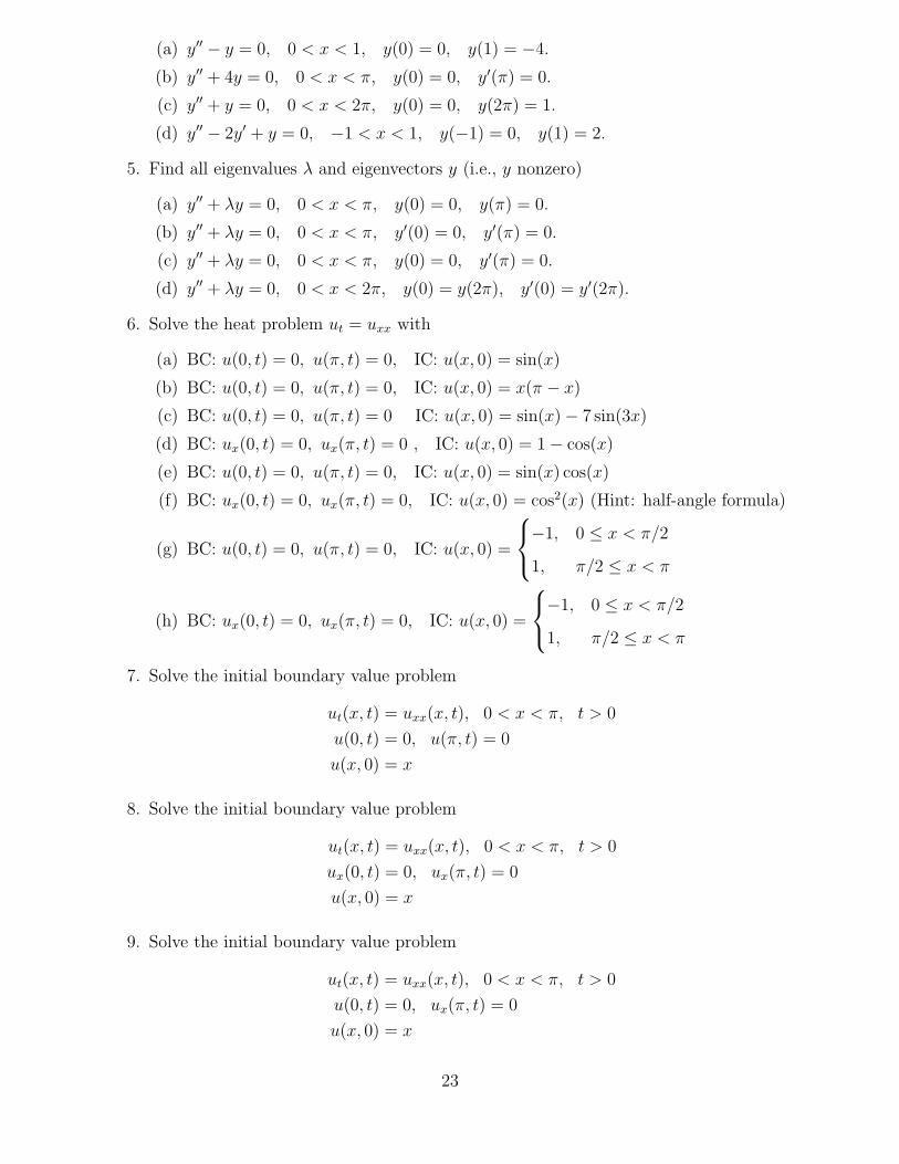
(a) y′′ − y = 0, 0 < x < 1, y(0) = 0, y(1) = −4.
(b) y′′ + 4y = 0, 0 < x < π, y(0) = 0, y′(π) = 0.
(c) y′′ + y = 0, 0 < x < 2π, y(0) = 0, y(2π) = 1.
(d) y′′ − 2y′ + y = 0, −1 < x < 1, y(−1) = 0, y(1) = 2.
5. Find all eigenvalues λ and eigenvectors y (i.e., y nonzero)
(a) y′′ + λy = 0, 0 < x < π, y(0) = 0, y(π) = 0.
(b) y′′ + λy = 0, 0 < x < π, y′(0) = 0, y′(π) = 0.
(c) y′′ + λy = 0, 0 < x < π, y(0) = 0, y′(π) = 0.
(d) y′′ + λy = 0, 0 < x < 2π, y(0) = y(2π), y′(0) = y′(2π).
6. Solve the heat problem ut = uxx with
(a) BC: u(0, t) = 0, u(π, t) = 0, IC: u(x, 0) = sin(x)
(b) BC: u(0, t) = 0, u(π, t) = 0, IC: u(x, 0) = x(π − x)
(c) BC: u(0, t) = 0, u(π, t) = 0 IC: u(x, 0) = sin(x)− 7 sin(3x)
(d) BC: ux(0, t) = 0, ux(π, t) = 0 , IC: u(x, 0) = 1− cos(x)
(e) BC: u(0, t) = 0, u(π, t) = 0, IC: u(x, 0) = sin(x) cos(x)
(f) BC: ux(0, t) = 0, ux(π, t) = 0, IC: u(x, 0) = cos2(x) (Hint: half-angle formula)
(g) BC: u(0, t) = 0, u(π, t) = 0, IC: u(x, 0) =
−1, 0 ≤ x < π/2
1, π/2 ≤ x < π
(h) BC: ux(0, t) = 0, ux(π, t) = 0, IC: u(x, 0) =
−1, 0 ≤ x < π/2
1, π/2 ≤ x < π
7. Solve the initial boundary value problem
ut(x, t) = uxx(x, t), 0 < x < π, t > 0
u(0, t) = 0, u(π, t) = 0
u(x, 0) = x
8. Solve the initial boundary value problem
ut(x, t) = uxx(x, t), 0 < x < π, t > 0
ux(0, t) = 0, ux(π, t) = 0
u(x, 0) = x
9. Solve the initial boundary value problem
ut(x, t) = uxx(x, t), 0 < x < π, t > 0
u(0, t) = 0, ux(π, t) = 0
u(x, 0) = x
23

10. Solve the initial boundary value problem
ut(x, t) = uxx(x, t)− 2ux(x, t), 0 < x < 1, t > 0
u(0, t) = 0, u(1, t) = 0
u(x, 0) = ex sin(πx)
11. Solve the initial boundary value problem
ut(x, t) = 2(uxx(x, t)− 3u(x, t)), 0 < x < 1, t > 0
u(0, t) = 0, u(1, t) = 0
u(x, 0) = 2 sin(πx)− 3 sin(2πx)
24