Embed Size (px)
Citation preview
3D UTAPWeLS Scripting Manual
Contents Introduction .................................................................................................................................................. 2
Installing Matlab Based 3D UTAPWeLS ..................................................................................................... 2
Starting Maltab Based 3D UTAPWeLS ...................................................................................................... 2
Backend Structure ......................................................................................................................................... 3
CSF ............................................................................................................................................................. 4
Well ........................................................................................................................................................... 5
Earth Model .............................................................................................................................................. 5
Log Set ....................................................................................................................................................... 8
Log ............................................................................................................................................................. 8
Nuclear Simulator ..................................................................................................................................... 8
Resistivity Simulator .................................................................................................................................. 9
Examples ..................................................................................................................................................... 11
Resistivity Simulation .............................................................................................................................. 11
Introduction When 3D UTAPWeLS is open using the Matlab Based version you get access to the backend of the
software. This means that from the Matlab command window, you can manipulate your data freely,
perform arbitrary calculations, use all of Matlab data visualization libraries, perform predefined 3D
UTAPWeLS calculations, manipulate your earth models, and run simulations on them.
Installing Matlab Based 3D UTAPWeLS First and foremost, make sure you have Matlab installed in your computer. We strongly recommend the
specific version 2015b; newer versions might work too.
Once you receive a zipped file from the 3D UTAPWeLS support group ([email protected]):
1. Unzip the zipped files “UTAPWeLS_MB_X.XX.zip” to a temporary directory.
2. Double-click on the startInstaller.bat file to open the installation wizard.
3. The installation wizard will ask you to choose an installation folder (please make sure you have
permissions to it), and will inquire whether you want to create a desktop shortcut.
4. Continue with the wizard instructions to complete the installation.
Starting Maltab Based 3D UTAPWeLS If you chose to create a desktop shortcut for the Matlab Based version of 3D UTAPWeLS, you can just
double click on it, and Matlab will open with the a CSF1 object called “utapCSF” loaded. This is your
backend entry point. Otherwise you can open Matlab (2015b) and type: “sessionObject = UTAPWeLS”;
this will start the program. To reach the backend entry point, now type: “utapCSF =
sessionObject.sessionData”.
1 Common Stratigraphic Framework
If you switch projects, you have switched your CSF object, so you need to get it again from the
“UTAPWeLS” session object. That is done simply by typing “utapCSF = sessionObject.sessionData”,
assuming you did not assign the variable name “sessionObject” to anything else.
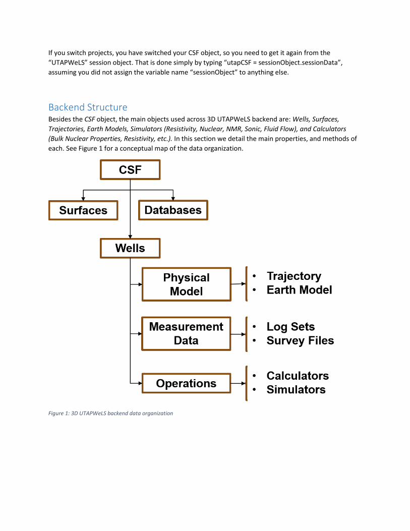
Backend Structure Besides the CSF object, the main objects used across 3D UTAPWeLS backend are: Wells, Surfaces,
Trajectories, Earth Models, Simulators (Resistivity, Nuclear, NMR, Sonic, Fluid Flow), and Calculators
(Bulk Nuclear Properties, Resistivity, etc.). In this section we detail the main properties, and methods of
each. See Figure 1 for a conceptual map of the data organization.
Figure 1: 3D UTAPWeLS backend data organization
It is also worth pointing out that the available properties and methods can always be found by using
Matlab’s tab completion: When you type the name of an object, followed by a dot, and press tab, a
selectable list of the available properties and functions will appear.
Most objects will have a name property which helps identify them. They also have the methods: delete
to remove itself (please use with care), and isvalid to check whether the object has been deleted.
Arguments in Methods
Different methods can take arguments in two different ways:
• Ordered Arguments: Where arguments are simply given as a set of values in a predetermined
order. Optional arguments are the last ones in the order. e. g.
csf.getWellByName(‘Well_1’)
• Paired Arguments: Arguments are specified as a set of argument-name, and argument-value
pairs. There is no specific order in which the arguments are given. This behavior is particularly
useful when there is a large number of optional arguments. e. g.
em.addBB(‘md’, 100, ‘unitMD’, ‘ft’)
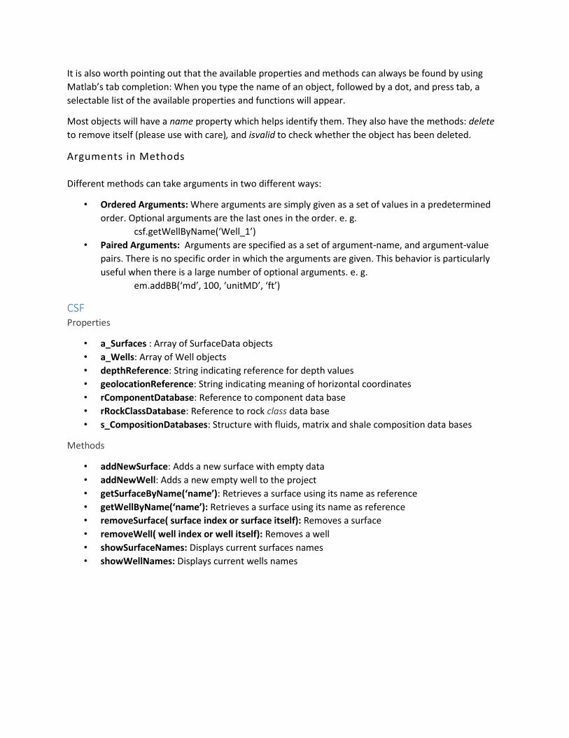
CSF Properties
• a_Surfaces : Array of SurfaceData objects
• a_Wells: Array of Well objects
• depthReference: String indicating reference for depth values
• geolocationReference: String indicating meaning of horizontal coordinates
• rComponentDatabase: Reference to component data base
• rRockClassDatabase: Reference to rock class data base
• s_CompositionDatabases: Structure with fluids, matrix and shale composition data bases
Methods
• addNewSurface: Adds a new surface with empty data
• addNewWell: Adds a new empty well to the project
• getSurfaceByName(‘name’): Retrieves a surface using its name as reference
• getWellByName(‘name’): Retrieves a surface using its name as reference
• removeSurface( surface index or surface itself): Removes a surface
• removeWell( well index or well itself): Removes a well
• showSurfaceNames: Displays current surfaces names
• showWellNames: Displays current wells names
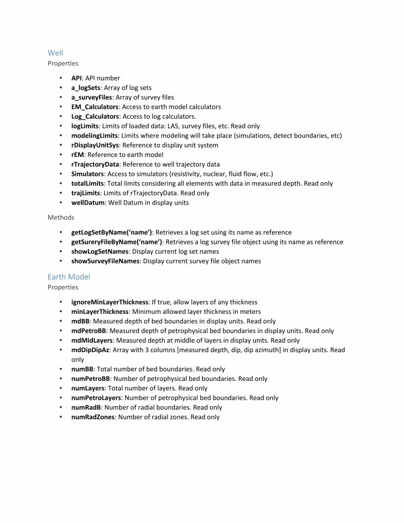
Well Properties
• API: API number
• a_logSets: Array of log sets
• a_surveyFiles: Array of survey files
• EM_Calculators: Access to earth model calculators
• Log_Calculators: Access to log calculators.
• logLimits: Limits of loaded data: LAS, survey files, etc. Read only
• modelingLimits: Limits where modeling will take place (simulations, detect boundaries, etc)
• rDisplayUnitSys: Reference to display unit system
• rEM: Reference to earth model
• rTrajectoryData: Reference to well trajectory data
• Simulators: Access to simulators (resistivity, nuclear, fluid flow, etc.)
• totalLimits: Total limits considering all elements with data in measured depth. Read only
• trajLimits: Limits of rTrajectoryData. Read only
• wellDatum: Well Datum in display units
Methods
• getLogSetByName(‘name’): Retrieves a log set using its name as reference
• getSureryFileByName(‘name’): Retrieves a log survey file object using its name as reference
• showLogSetNames: Display current log set names
• showSurveyFileNames: Display current survey file object names
Earth Model Properties
• ignoreMinLayerThickness: If true, allow layers of any thickness
• minLayerThickness: Minimum allowed layer thickness in meters
• mdBB: Measured depth of bed boundaries in display units. Read only
• mdPetroBB: Measured depth of petrophysical bed boundaries in display units. Read only
• mdMidLayers: Measured depth at middle of layers in display units. Read only
• mdDipDipAz: Array with 3 columns [measured depth, dip, dip azimuth] in display units. Read
only
• numBB: Total number of bed boundaries. Read only
• numPetroBB: Number of petrophysical bed boundaries. Read only
• numLayers: Total number of layers. Read only
• numPetroLayers: Number of petrophysical bed boundaries. Read only
• numRadB: Number of radial boundaries. Read only
• numRadZones: Number of radial zones. Read only
• radB: Radial boundaries. Read only
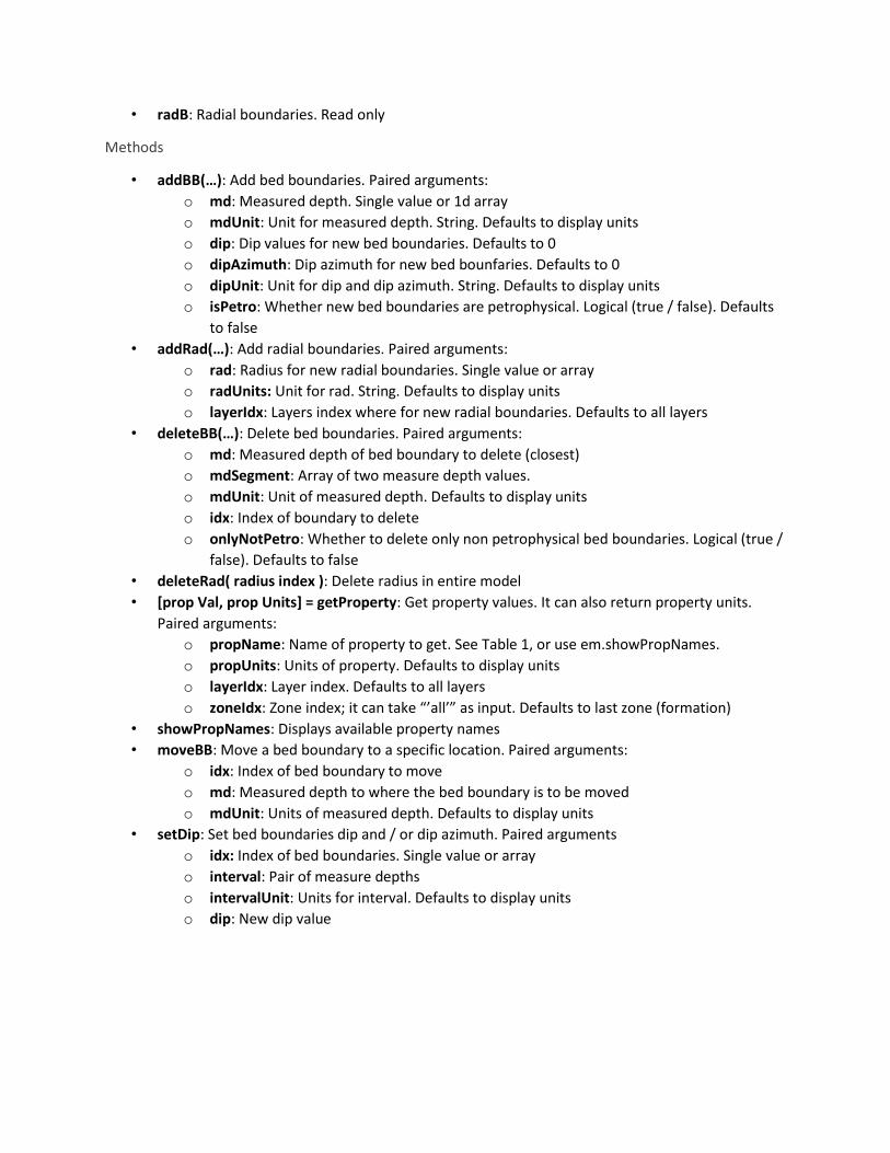
Methods
• addBB(…): Add bed boundaries. Paired arguments:
o md: Measured depth. Single value or 1d array
o mdUnit: Unit for measured depth. String. Defaults to display units
o dip: Dip values for new bed boundaries. Defaults to 0
o dipAzimuth: Dip azimuth for new bed bounfaries. Defaults to 0
o dipUnit: Unit for dip and dip azimuth. String. Defaults to display units
o isPetro: Whether new bed boundaries are petrophysical. Logical (true / false). Defaults
to false
• addRad(…): Add radial boundaries. Paired arguments:
o rad: Radius for new radial boundaries. Single value or array
o radUnits: Unit for rad. String. Defaults to display units
o layerIdx: Layers index where for new radial boundaries. Defaults to all layers
• deleteBB(…): Delete bed boundaries. Paired arguments:
o md: Measured depth of bed boundary to delete (closest)
o mdSegment: Array of two measure depth values.
o mdUnit: Unit of measured depth. Defaults to display units
o idx: Index of boundary to delete
o onlyNotPetro: Whether to delete only non petrophysical bed boundaries. Logical (true /
false). Defaults to false
• deleteRad( radius index ): Delete radius in entire model
• [prop Val, prop Units] = getProperty: Get property values. It can also return property units.
Paired arguments:
o propName: Name of property to get. See Table 1, or use em.showPropNames.
o propUnits: Units of property. Defaults to display units
o layerIdx: Layer index. Defaults to all layers
o zoneIdx: Zone index; it can take “’all’” as input. Defaults to last zone (formation)
• showPropNames: Displays available property names
• moveBB: Move a bed boundary to a specific location. Paired arguments:
o idx: Index of bed boundary to move
o md: Measured depth to where the bed boundary is to be moved
o mdUnit: Units of measured depth. Defaults to display units
• setDip: Set bed boundaries dip and / or dip azimuth. Paired arguments
o idx: Index of bed boundaries. Single value or array
o interval: Pair of measure depths
o intervalUnit: Units for interval. Defaults to display units
o dip: New dip value
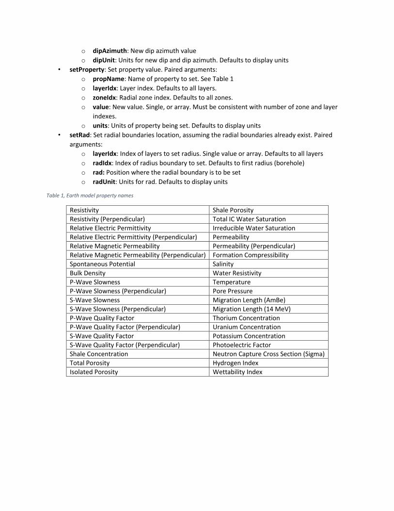
o dipAzimuth: New dip azimuth value
o dipUnit: Units for new dip and dip azimuth. Defaults to display units
• setProperty: Set property value. Paired arguments:
o propName: Name of property to set. See Table 1
o layerIdx: Layer index. Defaults to all layers.
o zoneIdx: Radial zone index. Defaults to all zones.
o value: New value. Single, or array. Must be consistent with number of zone and layer
indexes.
o units: Units of property being set. Defaults to display units
• setRad: Set radial boundaries location, assuming the radial boundaries already exist. Paired
arguments:
o layerIdx: Index of layers to set radius. Single value or array. Defaults to all layers
o radIdx: Index of radius boundary to set. Defaults to first radius (borehole)
o rad: Position where the radial boundary is to be set
o radUnit: Units for rad. Defaults to display units
Table 1, Earth model property names
Resistivity Shale Porosity
Resistivity (Perpendicular) Total IC Water Saturation
Relative Electric Permittivity Irreducible Water Saturation
Relative Electric Permittivity (Perpendicular) Permeability
Relative Magnetic Permeability Permeability (Perpendicular)
Relative Magnetic Permeability (Perpendicular) Formation Compressibility
Spontaneous Potential Salinity
Bulk Density Water Resistivity
P-Wave Slowness Temperature
P-Wave Slowness (Perpendicular) Pore Pressure
S-Wave Slowness Migration Length (AmBe)
S-Wave Slowness (Perpendicular) Migration Length (14 MeV)
P-Wave Quality Factor Thorium Concentration
P-Wave Quality Factor (Perpendicular) Uranium Concentration
S-Wave Quality Factor Potassium Concentration
S-Wave Quality Factor (Perpendicular) Photoelectric Factor
Shale Concentration Neutron Capture Cross Section (Sigma)
Total Porosity Hydrogen Index
Isolated Porosity Wettability Index
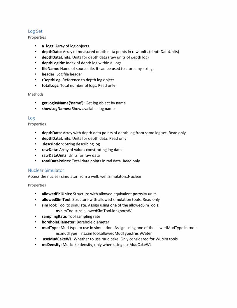
Log Set Properties
• a_logs: Array of log objects.
• depthData: Array of measured depth data points in raw units (depthDataUnits)
• depthDataUnits: Units for depth data (raw units of depth log)
• depthLogIdx: Index of depth log within a_logs
• fileName: Name of source file. It can be used to store any string
• header: Log file header
• rDepthLog: Reference to depth log object
• totalLogs: Total number of logs. Read only
Methods
• getLogByName(‘name’): Get log object by name
• showLogNames: Show available log names
Log Properties
• depthData: Array with depth data points of depth log from same log set. Read only
• depthDataUnits: Units for depth data. Read only
• description: String describing log
• rawData: Array of values constituting log data
• rawDataUnits: Units for raw data
• totalDataPoints: Total data points in rad data. Read only
Nuclear Simulator Access the nuclear simulator from a well: well.Simulators.Nuclear
Properties
• allowedPhiUnits: Structure with allowed equivalent porosity units
• allowedSimTool: Structure with allowed simulation tools. Read only
• simTool: Tool to simulate. Assign using one of the allowedSimTools:
ns.simTool = ns.allowedSimTool.longhornWL
• samplingRate: Tool sampling rate
• boreholeDiameter: Borehole diameter
• mudType: Mud type to use in simulation. Assign using one of the allwedMudType in tool:
ns.mudType = ns.simTool.allowedMudType.freshWater
• useMudCakeWL: Whether to use mud cake. Only considered for WL sim tools
• mcDensity: Mudcake density, only when using useMudCakeWL
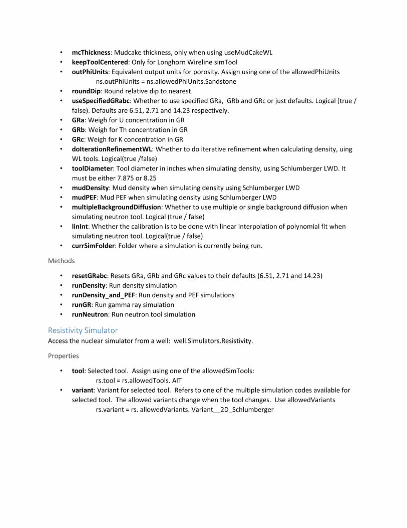
• mcThickness: Mudcake thickness, only when using useMudCakeWL
• keepToolCentered: Only for Longhorn Wireline simTool
• outPhiUnits: Equivalent output units for porosity. Assign using one of the allowedPhiUnits
ns.outPhiUnits = ns.allowedPhiUnits.Sandstone
• roundDip: Round relative dip to nearest.
• useSpecifiedGRabc: Whether to use specified GRa, GRb and GRc or just defaults. Logical (true /
false). Defaults are 6.51, 2.71 and 14.23 respectively.
• GRa: Weigh for U concentration in GR
• GRb: Weigh for Th concentration in GR
• GRc: Weigh for K concentration in GR
• doIterationRefinementWL: Whether to do iterative refinement when calculating density, uing
WL tools. Logical(true /false)
• toolDiameter: Tool diameter in inches when simulating density, using Schlumberger LWD. It
must be either 7.875 or 8.25
• mudDensity: Mud density when simulating density using Schlumberger LWD
• mudPEF: Mud PEF when simulating density using Schlumberger LWD
• multipleBackgroundDiffusion: Whether to use multiple or single background diffusion when
simulating neutron tool. Logical (true / false)
• linInt: Whether the calibration is to be done with linear interpolation of polynomial fit when
simulating neutron tool. Logical(true / false)
• currSimFolder: Folder where a simulation is currently being run.
Methods
• resetGRabc: Resets GRa, GRb and GRc values to their defaults (6.51, 2.71 and 14.23)
• runDensity: Run density simulation
• runDensity_and_PEF: Run density and PEF simulations
• runGR: Run gamma ray simulation
• runNeutron: Run neutron tool simulation
Resistivity Simulator Access the nuclear simulator from a well: well.Simulators.Resistivity.
Properties
• tool: Selected tool. Assign using one of the allowedSimTools:
rs.tool = rs.allowedTools. AIT
• variant: Variant for selected tool. Refers to one of the multiple simulation codes available for
selected tool. The allowed variants change when the tool changes. Use allowedVariants
rs.variant = rs. allowedVariants. Variant__2D_Schlumberger
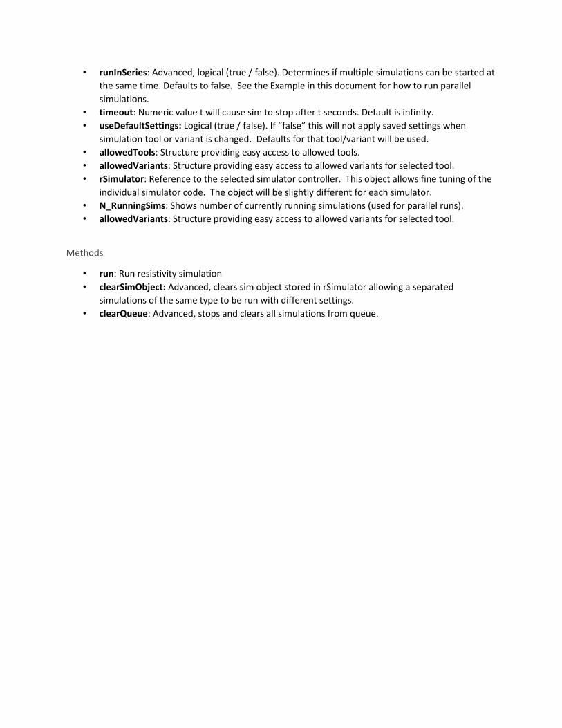
• runInSeries: Advanced, logical (true / false). Determines if multiple simulations can be started at
the same time. Defaults to false. See the Example in this document for how to run parallel
simulations.
• timeout: Numeric value t will cause sim to stop after t seconds. Default is infinity.
• useDefaultSettings: Logical (true / false). If “false” this will not apply saved settings when
simulation tool or variant is changed. Defaults for that tool/variant will be used.
• allowedTools: Structure providing easy access to allowed tools.
• allowedVariants: Structure providing easy access to allowed variants for selected tool.
• rSimulator: Reference to the selected simulator controller. This object allows fine tuning of the
individual simulator code. The object will be slightly different for each simulator.
• N_RunningSims: Shows number of currently running simulations (used for parallel runs).
• allowedVariants: Structure providing easy access to allowed variants for selected tool.
Methods
• run: Run resistivity simulation
• clearSimObject: Advanced, clears sim object stored in rSimulator allowing a separated
simulations of the same type to be run with different settings.
• clearQueue: Advanced, stops and clears all simulations from queue.
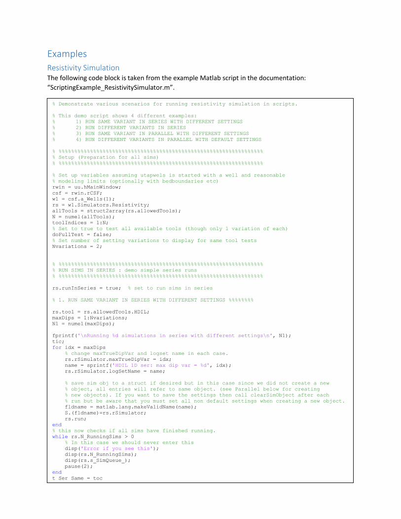
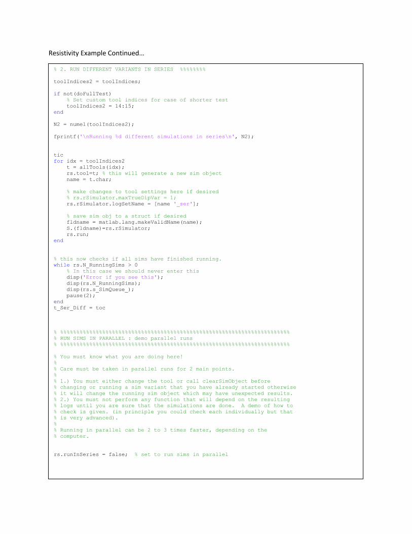
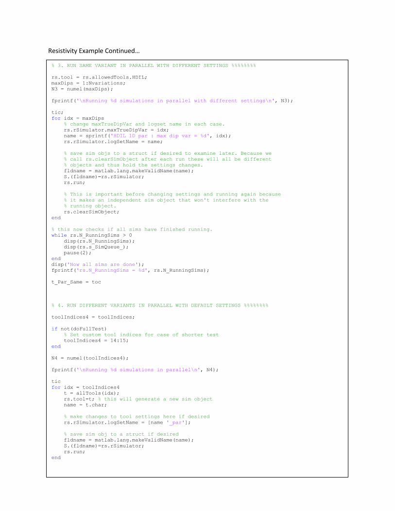
Examples
Resistivity Simulation The following code block is taken from the example Matlab script in the documentation:
“ScriptingExample_ResistivitySimulator.m”.
% Demonstrate various scenarios for running resistivity simulation in scripts.
% This demo script shows 4 different examples:
% 1) RUN SAME VARIANT IN SERIES WITH DIFFERENT SETTINGS
% 2) RUN DIFFERENT VARIANTS IN SERIES
% 3) RUN SAME VARIANT IN PARALLEL WITH DIFFERENT SETTINGS
% 4) RUN DIFFERENT VARIANTS IN PARALLEL WITH DEFAULT SETTINGS
% %%%%%%%%%%%%%%%%%%%%%%%%%%%%%%%%%%%%%%%%%%%%%%%%%%%%%%%%%%%%%%%%%
% Setup (Preparation for all sims)
% %%%%%%%%%%%%%%%%%%%%%%%%%%%%%%%%%%%%%%%%%%%%%%%%%%%%%%%%%%%%%%%%%
% Set up variables assuming utapwels is started with a well and reasonable
% modeling limits (optionally with bedboundaries etc)
rwin = uu.hMainWindow;
csf = rwin.rCSF;
w1 = csf.a_Wells(1);
rs = w1.Simulators.Resistivity;
allTools = struct2array(rs.allowedTools);
N = numel(allTools);
toolIndices = 1:N;
% Set to true to test all available tools (though only 1 variation of each)
doFullTest = false;
% Set number of setting variations to display for same tool tests
Nvariations = 2;
% %%%%%%%%%%%%%%%%%%%%%%%%%%%%%%%%%%%%%%%%%%%%%%%%%%%%%%%%%%%%%%%%%
% RUN SIMS IN SERIES : demo simple series runs
% %%%%%%%%%%%%%%%%%%%%%%%%%%%%%%%%%%%%%%%%%%%%%%%%%%%%%%%%%%%%%%%%%
rs.runInSeries = true; % set to run sims in series
% 1. RUN SAME VARIANT IN SERIES WITH DIFFERENT SETTINGS %%%%%%%%
rs.tool = rs.allowedTools.HDIL;
maxDips = 1:Nvariations;
N1 = numel(maxDips);
fprintf('\nRunning %d simulations in series with different settings\n', N1);
tic;
for idx = maxDips
% change maxTrueDipVar and logset name in each case.
rs.rSimulator.maxTrueDipVar = idx;
name = sprintf('HDIL 1D ser: max dip var = %d', idx);
rs.rSimulator.logSetName = name;
% save sim obj to a struct if desired but in this case since we did not create a new
% object, all entries will refer to same object. (see Parallel below for creating
% new objects). If you want to save the settings then call clearSimObject after each
% run but be aware that you must set all non default settings when creating a new object.
fldname = matlab.lang.makeValidName(name);
S.(fldname)=rs.rSimulator;
rs.run;
end
% this now checks if all sims have finished running.
while rs.N_RunningSims > 0
% In this case we should never enter this
disp('Error if you see this');
disp(rs.N_RunningSims);
disp(rs.s_SimQueue_);
pause(2);
end
t_Ser_Same = toc
% 2. RUN DIFFERENT VARIANTS IN SERIES %%%%%%%%
Resistivity Example Continued…
% 2. RUN DIFFERENT VARIANTS IN SERIES %%%%%%%%
toolIndices2 = toolIndices;
if not(doFullTest)
% Set custom tool indices for case of shorter test
toolIndices2 = 14:15;
end
N2 = numel(toolIndices2);
fprintf('\nRunning %d different simulations in series\n', N2);
tic
for idx = toolIndices2
t = allTools(idx);
rs.tool=t; % this will generate a new sim object
name = t.char;
% make changes to tool settings here if desired
% rs.rSimulator.maxTrueDipVar = 1;
rs.rSimulator.logSetName = [name '_ser'];
% save sim obj to a struct if desired
fldname = matlab.lang.makeValidName(name);
S.(fldname)=rs.rSimulator;
rs.run;
end
% this now checks if all sims have finished running.
while rs.N_RunningSims > 0
% In this case we should never enter this
disp('Error if you see this');
disp(rs.N_RunningSims);
disp(rs.s_SimQueue_);
pause(2);
end
t_Ser_Diff = toc
% %%%%%%%%%%%%%%%%%%%%%%%%%%%%%%%%%%%%%%%%%%%%%%%%%%%%%%%%%%%%%%%%%%%%%%%
% RUN SIMS IN PARALLEL : demo parallel runs
% %%%%%%%%%%%%%%%%%%%%%%%%%%%%%%%%%%%%%%%%%%%%%%%%%%%%%%%%%%%%%%%%%%%%%%%
% You must know what you are doing here!
%
% Care must be taken in parallel runs for 2 main points.
%
% 1.) You must either change the tool or call clearSimObject before
% changing or running a sim variant that you have already started otherwise
% it will change the running sim object which may have unexpected results.
% 2.) You must not perform any function that will depend on the resulting
% logs until you are sure that the simulations are done. A demo of how to
% check is given. (in principle you could check each individually but that
% is very advanced).
%
% Running in parallel can be 2 to 3 times faster, depending on the
% computer.
rs.runInSeries = false; % set to run sims in parallel
% 3. RUN SAME VARIANT IN PARALLEL WITH DIFFERENT SETTINGS %%%%%%%%
rs.tool = rs.allowedTools.HDIL;
maxDips = 1:Nvariations;
N3 = numel(maxDips);
fprintf('\nRunning %d simulations in parallel with different settings\n', N3);
tic;
for idx = maxDips
% change maxTrueDipVar and logset name in each case.
Resistivity Example Continued…
% 3. RUN SAME VARIANT IN PARALLEL WITH DIFFERENT SETTINGS %%%%%%%%
rs.tool = rs.allowedTools.HDIL;
maxDips = 1:Nvariations;
N3 = numel(maxDips);
fprintf('\nRunning %d simulations in parallel with different settings\n', N3);
tic;
for idx = maxDips
% change maxTrueDipVar and logset name in each case.
rs.rSimulator.maxTrueDipVar = idx;
name = sprintf('HDIL 1D par : max dip var = %d', idx);
rs.rSimulator.logSetName = name;
% save sim objs to a struct if desired to examine later. Because we
% call rs.clearSimObject after each run these will all be different
% objects and thus hold the settings changes.
fldname = matlab.lang.makeValidName(name);
S.(fldname)=rs.rSimulator;
rs.run;
% This is important before changing settings and running again because
% it makes an independent sim object that won't interfere with the
% running object.
rs.clearSimObject;
end
% this now checks if all sims have finished running.
while rs.N_RunningSims > 0
disp(rs.N_RunningSims);
disp(rs.s_SimQueue_);
pause(2);
end
disp('Now all sims are done');
fprintf('rs.N_RunningSims = %d', rs.N_RunningSims);
t_Par_Same = toc
% 4. RUN DIFFERENT VARIANTS IN PARALLEL WITH DEFAULT SETTINGS %%%%%%%%
toolIndices4 = toolIndices;
if not(doFullTest)
% Set custom tool indices for case of shorter test
toolIndices4 = 14:15;
end
N4 = numel(toolIndices4);
fprintf('\nRunning %d simulations in parallel\n', N4);
tic
for idx = toolIndices4
t = allTools(idx);
rs.tool=t; % this will generate a new sim object
name = t.char;
% make changes to tool settings here if desired
rs.rSimulator.logSetName = [name '_par'];
% save sim obj to a struct if desired
fldname = matlab.lang.makeValidName(name);
S.(fldname)=rs.rSimulator;
rs.run;
end
fprintf(...
'Running %d runs of same variant in series took %f sec\n', ...
Resistivity Example Continued…
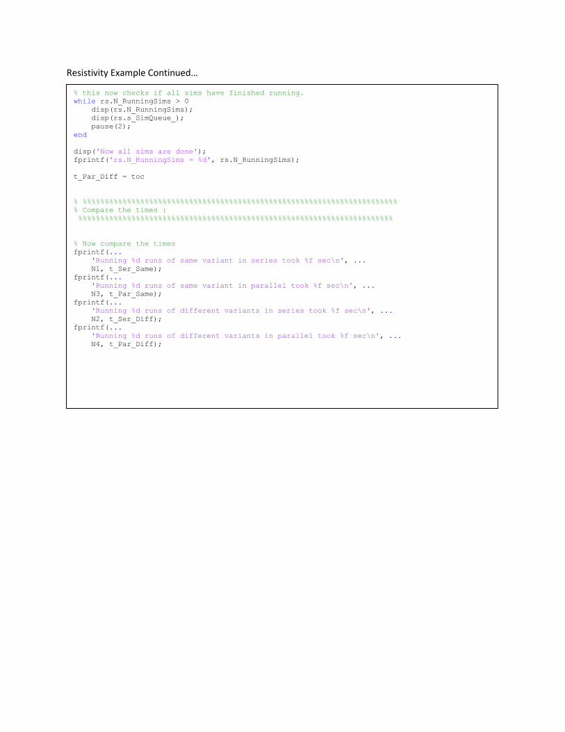
% this now checks if all sims have finished running.
while rs.N_RunningSims > 0
disp(rs.N_RunningSims);
disp(rs.s_SimQueue_);
pause(2);
end
disp('Now all sims are done');
fprintf('rs.N_RunningSims = %d', rs.N_RunningSims);
t_Par_Diff = toc
% %%%%%%%%%%%%%%%%%%%%%%%%%%%%%%%%%%%%%%%%%%%%%%%%%%%%%%%%%%%%%%%%%%%%%%%
% Compare the times :
%%%%%%%%%%%%%%%%%%%%%%%%%%%%%%%%%%%%%%%%%%%%%%%%%%%%%%%%%%%%%%%%%%%%%%%
% Now compare the times
fprintf(...
'Running %d runs of same variant in series took %f sec\n', ...
N1, t_Ser_Same);
fprintf(...
'Running %d runs of same variant in parallel took %f sec\n', ...
N3, t_Par_Same);
fprintf(...
'Running %d runs of different variants in series took %f sec\n', ...
N2, t_Ser_Diff);
fprintf(...
'Running %d runs of different variants in parallel took %f sec\n', ...
N4, t_Par_Diff);