3D ultrafast echocardiography: toward a quantitative

HAL Id: tel-02373882https://tel.archives-ouvertes.fr/tel-02373882

Submitted on 21 Nov 2019

HAL is a multi-disciplinary open accessarchive for the deposit and dissemination of sci-entific research documents, whether they are pub-lished or not. The documents may come fromteaching and research institutions in France orabroad, or from public or private research centers.

L’archive ouverte pluridisciplinaire HAL, estdestinée au dépôt et à la diffusion de documentsscientifiques de niveau recherche, publiés ou non,émanant des établissements d’enseignement et derecherche français ou étrangers, des laboratoirespublics ou privés.

3D ultrafast echocardiography : toward a quantitativeimaging of the myocardium.

Victor Finel

To cite this version:Victor Finel. 3D ultrafast echocardiography : toward a quantitative imaging of the myocardium..Physics [physics]. Université Sorbonne Paris Cité, 2018. English. �NNT : 2018USPCC134�. �tel-02373882�

https://tel.archives-ouvertes.fr/tel-02373882

https://hal.archives-ouvertes.fr

Thèse de Doctorat

De l’Université Sorbonne Paris Cité

Préparée à l’Université Paris Diderot

Ecole doctorale 564 : Physique en Ile de France

Laboratoire : Institut Langevin

3D ultrafast echocardiography:

Toward a quantitative imaging of the

myocardium

Victor Finel

Thèse de doctorat d’Acoustique Physique

Dirigée par Mathieu Pernot

Présentée et soutenue publiquement à Paris le 15 Novembre 2018

Membres du jury

Présidente du jury : Prada, Claire / Directrice de Recherche / Institut Langevin, CNRS

Rapporteurs : - Catheline, Stefan / Directeur de Recherche / Labtau, INSERM

- Jan D’Hooge / Professeur des Universités / KU Leuven

Examinatrice : Francesca Raimondi Vidoli / Praticien Hospitalier / Hôpital Necker Enfants Malades, APHP

Directeur de thèse : Mathieu Pernot / Directeur de Recherche / Institut Langevin, INSERM

Co-directeur de thèse : Mickaël Tanter / Directeur de Recherche / Institut Langevin, INSERM

2

3

Acknowledgments Tout d’abord, je tiens à remercier chaleureusement mes directeurs de thèse, Mathieu Pernot et Mickaël Tanter, de m’avoir offert l’opportunité d’effectuer ces travaux. Ce fut une expérience formidable de pouvoir profiter de leur vision de la recherche, qui permet à nous autres doctorants de travailler sur des sujets passionnants, prometteurs, de bénéficier de superbes outils pour ce faire, et d’aller présenter nos travaux ici et là. Sans oublier ces quelques semaines en Uruguay. Mathieu, Micka, merci pour votre foie scientifique indestructible !

Merci à Stefan Catheline et Jan D’hooge, qui ont accepté de rapporter ces travaux, et merci à Francesca Raimondi Vidoli et Claire Prada, qui se sont jointes au jury.

Au long de cette thèse, plusieurs collaborations ont été effectuées, qui ont été autant de belles rencontres. Merci à Zak et Xav de l’équipe de Bordeaux, Francesca de Necker, gracias Javier, Carlos, Nicasio, Thomas, Daniel de Montevideo (por todo y en particular por los asados…).

Merci à Guillaume Renaud, qui m’a fait découvrir les ultrasons pour la médecine, et qui a été mon tuteur scientifique depuis.

Il y a également énormément de personnes à remercier à l’institut Langevin, sans qui le labo s’écroulerait tout simplement. Merci Khadija pour toutes les tâches incroyables que tu fais, sans oublier le coaching pour la rédaction de ce mémoire. Merci Patricia pour l’organisation sans faille du « petit matériel » sans lequel rien n’est possible, et surtout, merci d’avoir été ma marraine pendant ces trois années. Merci à Jean de m’avoir introduit en tout premier lieu au labo pour mon stage, et de m’avoir retourné le cerveau lorsque j’ai découvert le monde de l’échographie (ultrarapide, cela va de soi), les LegHal, et les codes optimisés. Merci à Mafalda de m’avoir présenté à LA machine 3D, et pour les longues sessions de travail en commun qui en ont découlées. Merci à Olo pour les heures de manips, de traitement de données, et de m’avoir tout appris de ce que je sais en cardiologie aujourd’hui. Merci à Clément pour ses conseils au labo mais aussi à l’éxtérieur, qui m’ont appris l’art du moyennage et de la négociation. Merci à Philippe M. et ses doigts de fées qui m’offrirent de superbes manips. Merci Emmanuel pour les discussions, les échanges sur le traitement d’image et le fast marching, sans oublier les fallafels. Merci à Hicham pour ses encouragements aveugles et les conseils aussi variés qu’enrichissants. Merci à Philippe A. et Alex pour leurs expertises en électronique et informatique (promis je ne crasherai plus gitlab).

Merci aussi à ceux avec qui nous avons partagés plus qu’un bureau : Martin (surtout pour les tracteurs), Thomas, Daniel, Momo, Florian, Mafalda, Claudia, Emmanuel, Pauline et Pauline (même si t’es partie bien vite). Merci à Guillaume M de m’avoir fait tant suer à te courir après, et à la team jogging qui s’est agrandie. On n’a pas partagé de bureau, mais quand même de superbes moments : merci Claire, Elliot, Line, Marc, Baptiste et Baptiste, Béa, Alex D, Mai, Jack, Charlie, Thomas D, Charlotte, Ludovic, Vincent, Jérôme, Marion, Justine, … Pensée émue pour les nombreux karaokés, les nerfs, et NY.

4

Merci aussi à toute l’équipe de la Cité des Sciences, avec qui ce fut un réel plaisir de travailler, mais aussi d’avoir des discussions passionnantes (et merci pour les lunettes). Merci Fawzila, Olivier, Nadège, JB, Morgane, Alain, Gilles, Anaïs, Aurélie, Valérie, Marlène, Julia, Hélène, Laeticia, Graziela, Mathieu.

Merci à Simon sans qui le temps (-réel et de sauvegarde) ne serait pas pareil. Merci à Charles de m’avoir montré le chemin de la Suède et de l’acoustique, à Thomas de m’avoir apporté concrètement plein de choses. Merci aux copains et colocs qui ont supportés les aléas des humeurs d’un thésard et qui m’ont encouragé. Merci à ceux qui brûlent !

Merci à ma famille qui a toujours cru en moi.

5

Abstract The objectives of this PhD thesis were to develop 3D ultrafast ultrasound imaging of the human heart toward the characterization of cardiac tissues. In order to do so, a customized, programmable, ultrafast scanner built in our group was used. In the first part of this thesis, a real-time imaging sequence was developed to facilitate in-vivo imaging using this scanner, as well as dedicated 3D and 4D visualization tools.

Then, we developed 3D Backscatter Tensor Imaging (BTI), a technique to visualize the muscular fibres orientation within the heart wall non-invasively during the cardiac cycle. Applications on a healthy volunteer before and after cardiac contraction were shown. Moreover, the undesired effects of axial motion on BTI were studied, and a methodology to estimate motion velocity and reduce the undesired effects was introduced and applied on a healthy volunteer. This technique may become an interesting tool for the diagnosis and quantification of fibres disarrays in hypertrophic cardiomyopathies.

Moreover, 3D ultrafast ultrasound was used to image the propagation of naturally generated elastic waves in the heart walls, and an algorithm to determine their speed was developed. The technique was validated in silico and the in vivo feasibility was shown on two healthy volunteers, during cardiac contraction and relaxation. As the velocity of elastic waves is directly related to the rigidity of the heart, this technique could be a way to assess the ability of the ventricle to contract and relax, which is an important parameter for cardiac function evaluation.

Finally, the transient myocardial contraction was imaged in 3D on isolated rat hearts at high framerate in order to analyse the activation sequence. Mechanical activation delays were successfully quantified during natural rhythm, pacing and hypothermia. Then, the feasibility of the technique in 2D non-invasively on human hearts was investigated. Applications on foetuses and adults hearts were shown. This imaging technique may help the characterization of cardiac arrhythmias, and thus improve their treatment.

In conclusion, we have introduced in this work three novel 3D ultrafast imaging modalities for the quantification of structural and functional myocardial properties. 3D ultrafast imaging may become an important non-ionizing, transportable diagnostic tool that may improve the patient care at the bed side.

Keywords: ultrafast ultrasound imaging, echocardiography, cardiac imaging, 3D imaging, myocardium characterization

6

Résumé L’objectif de cette thèse de doctorat était de développer l’échographie ultrarapide 3D du cœur, plus particulièrement dans le but de caractériser le muscle cardiaque. A cet effet, un échographe ultrarapide assemblé dans notre laboratoire a été utilisé. Dans la première partie de cette thèse, un mode d’imagerie temps-réel a été développé pour faciliter l’imagerie in-vivo en utilisant ce scanner, ainsi que des outils de visualisation 3D et 4D.

Par la suite, l’imagerie 3D du tenseur de rétrodiffusion a été développée pour analyser l’orientation des fibres musculaires du cœur de manière non-invasive et au cours du cycle cardiaque. Des résultats ont été obtenus sur un volontaire avant et après la contraction cardiaque. De plus, les effets indésirables du mouvement axial ont été étudiés, et une méthode d’estimation de la vitesse axiale et de correction des aberrations induites a été proposée et appliquée sur l’homme. Cette technique pourrait devenir un outil intéressant de diagnostic et quantification de la désorganisation des fibres musculaires dans le cadre de cardiomyopathies hypertrophiques.

De plus, l’échographie ultrarapide 3D a été utilisée pour visualiser la propagation dans les parois du cœur d’ondes élastiques générées naturellement au cours du cycle cardiaque, et un algorithme pour déterminer leurs vitesses a été développé. Cette technique a été validée grâce à des simulations numériques puis appliquée sur deux volontaires sains, pendant les phases de contraction et relaxation du myocarde. Etant donné que la vitesse des ondes de cisaillement est directement reliée à la rigidité du cœur, cette méthode pourrait permettre d’estimer la capacité du cœur à se contracter et à se relâcher, qui sont des paramètres important pour son fonctionnement.

Enfin, l’activation de la contraction cardiaque de cœurs de rats isolés a été imagée à haute cadence et en 3D dans le but d’analyser la synchronisation de la contraction. Les délais d’activation mécanique ont pu correctement être quantifiés lors du rythme naturel du cœur, de stimulations électriques extérieures ainsi qu’en hypothermie. Ensuite, la faisabilité de la technique en 2D sur des cœurs humains de manière non-invasive a été étudiée et appliquée sur des fœtus et des adultes. Cette technique d’imagerie pourrait aider la caractérisation d’arythmies et améliorer leur traitement.

En conclusion, nous avons introduit dans ces travaux de thèse trois nouvelles modalités d’imagerie ultrarapide 3D permettant de quantifier des propriétés structurelles et fonctionnelles du myocarde, qui jusqu’ici ne pouvaient pas être imagée en échocardiographie. L’imagerie 3D ultrarapide est une modalité très prometteuse, non ionisante, transportable et qui pourrait dans le futur améliorer fortement le diagnostic et la prise en charge des patients.

Mots-clés: imagerie ultrarapide par ultrasons, échocardiographie, imagerie cardiaque, imagerie 3D, caractérisation du myocarde

7

Résumé détaillé Chapitre 1 : Introduction

Cher lecteur, il y a une chance sur trois que vous mourriez d’une maladie cardiovasculaire. Telles sont les statistiques de l’Organisation Mondiale de la Santé : les maladies cardiovasculaires sont la principale cause de mortalité mondiale, responsables d’environ un tiers des décès, et sans surprises, leur détection précoce est un élément clé pour mieux les guérir. Dans ce contexte, un important travail de recherche est fait mondialement pour améliorer les techniques d’imagerie cardiaque, et cette thèse espère apporter sa petite pierre à l’édifice.

Dans le premier chapitre, une description rapide des techniques d’imagerie actuelles sera donnée, avec un accent particulier sur l’échographie. Parmi ses plus récents développements, nous porterons notre intérêt sur l’échographie ultrarapide, car cette technique sera fondamentale dans la suite. Dans le second chapitre, nous présenterons l’échographie ultrarapide 3D, qui sera utilisée tout au long de ces travaux, ainsi que les outils dédiés développés pour visualiser des données 3D et 4D (3D+temps). Le troisième chapitre sera consacré à l’imagerie 3D de l’orientation des fibres musculaires composant le cœur. Des applications sur l’homme seront montrées, ainsi qu’une étude visant à estimer les artefacts créés par le mouvement sur les résultats, puis un algorithme pour les corriger. Par la suite, le quatrième chapitre montrera comment mesurer de manière passive, en 3D et à différents instants du cycle cardiaque la rigidité du cœur. Enfin, dans le cinquième chapitre, l’échographie ultrarapide 3D sera utilisée pour imager la séquence d’activation de la contraction cardiaque.

Les cardiologues possèdent aujourd’hui un vaste panel d’outils pour étudier le fonctionnement du cœur. L’ECG est probablement le plus connu d’entre eux : il permet d’obtenir une trace de l’activité électrique du cœur mesurée sur le torse des patients. Cependant, il ne permet pas d’imager à proprement parler d’où viennent les signaux électriques. D’autres techniques sont donc nécessaires pour obtenir une image : IRM, rayons X, traceurs radioactifs, ultrasons, etc.. Chacune d’entre elles a des avantages et des inconvénients, et en particulier, l’échographie a l’atout d’être non-invasive, non-ionisante, moins chère et donc plus accessible. Différents modes d’imagerie existent : il est ainsi possible de visualiser l’anatomie (B-Mode), les flux sanguins (modes Doppler), ou encore la contraction musculaire (strain imaging). Cependant, les ultrasons ont aussi un certain nombre d’inconvénients, et parmi eux, nous retiendrons particulièrement la limitation à des images 2D qui compliquent la visualisation de structures ou phénomènes complexes intrinsèquement 3D. Ces dernières années ont vu l’apparition d’échographe 3D, mais la cadence d’imagerie accessible (de l’ordre d’une dizaine de frames par seconde), n’est pas suffisante pour imager les phénomènes cardiaque rapides.

Les récentes recherches en échographie ont permis de lever ces limites : ainsi, l’échographie ultrarapide a permis d’accéder à des cadences jusqu’à 10 000 images/secondes, aussi bien en 2D qu’en 3D. A l’heure actuelle, les applications de l’échographie 3D ultrarapide sont encore en pleine phase de recherche. Les objectifs de cette thèse étaient donc de développer l’échographie cardiaque 3D ultrarapide et plus particulièrement de l’appliquer à l’étude du myocarde.

8

Chapitre 2 : l’échographie ultrarapide 3D

L’échographie ultrarapide, qu’elle soit 2D ou 3D, repose sur la capacité de contrôler simultanément tous les éléments des sondes échographiques (une centaine de voies en 2D, et jusqu’à un millier pour la 3D), et a donc été un challenge technologique, qui n’a été relevé qu’à l’aube des années 2000 pour les images 2D et 2010 pour la 3D. Ainsi, ces travaux de thèse ont été effectués à l’aide d’un prototype d’échographe 3D ultrarapide développé au sein du laboratoire, et qui à l’origine, ne permettait pas d’obtenir des images en temps-réel. Nous avons donc créé une modalité d’imagerie temps-réel en utilisant cet échographe et les sondes matricielles associées, une fonctionnalité essentielle pour pouvoir étudier le vivant. Une technique d’émission focalisant les ultrasons dans le plan d’imagerie a été conçue pour fournir une image 2D temps-réel de qualité, permettant au clinicien d’obtenir le champ de vue souhaité avant de déclencher une acquisition 3D ultrarapide.

Une fois les images 3D obtenues, se pose la question de leur visualisation. De nombreux outils dédiés existent déjà mais cependant, nous souhaitions pouvoir explorer les données rapidement, de manière automatisée et dans l’environnement MATLAB. Dans ce but, plusieurs fonctions 3D ont été développées : l’une dédiée à la visualisation de l’orientation des fibres musculaires, l’autre à la visualisation des parois du cœur. Enfin, une fonctionnalité additionnelle permettant de contrôler le temps tout en utilisant une fonction de visualisation a été créée.

Chapitre 3 : Imagerie 3D du tenseur de rétrodiffusion

La première partie de ce chapitre est dédiée à l’imagerie de l’anisotropie des tissus biologiques par imagerie du tenseur de rétrodiffusion (en anglais, Backscatter Tensor Imaging, abrégé BTI). Les fibres musculaires sont structurées de manière hélicoïdale à travers la paroi cardiaque, de manière à ce que leurs contractions entrainent l’éjection du sang dans un mouvement de torsion et de contraction des ventricules. Ainsi, l’agencement des fibres influe directement la capacité d’éjection du sang du cœur, et est mise à défaut dans des pathologies comme l’hypertrophie myocardique. L’imagerie de l’orientation des fibres cardiaques pourrait donc être intéressante pour la détection précoce et le suivi de ces pathologies.

Définissons l’axe Z comme étant la profondeur des tissus imagés : dans ce cas, si ces derniers sont anisotropes dans le plan XY, le théorème de Van Cittert Zernike stipule que la cohérence des échos rétrodiffusés dans un plan XY parallèle sera également anisotrope. Ainsi dans le cas d’un milieu fibreux, la cohérence sera plus forte dans la direction des fibres que dans la direction perpendiculaire à celles-ci. L’utilisation d’une sonde échographique matricielle permet de calculer directement la cohérence des échos mesurés dans un tel plan. De plus, en utilisant l’échographie ultrarapide, cette mesure peut être obtenue dans tous les points du volume avec une bonne cadence d’imagerie (de l’ordre de 90 volumes/seconde), ce qui permet d’imager l’orientation des fibres au cours du temps en un unique battement cardiaque.

Ainsi, la première partie de ce chapitre démontre comment a été créée une séquence d’émissions d’ultrasons pour le BTI, la mise en place des calculs de cohérence pour chaque voxel et de l’analyse des fonctions de cohérence 2D obtenues pour en déduire leurs éventuelles anisotropies

9

et leurs directions, puis une démonstration du BTI pour imager l’orientation des fibres musculaires de la paroi antéro-septale du cœur d’un volontaire sain est présentée.

Ensuite, l’impact du mouvement sur les calculs de fonction de cohérence a été étudié. En effet, le BTI 3D repose sur la focalisation synthétique par onde planes, technique sous-jacente de l’échographie ultrarapide, qui suppose que les mouvements des tissus imagés sont négligeables. Hors, ce n’est pas vrai dans le cas du cœur : dans la deuxième partie de ce chapitre, nous avons mis en évidence les artefacts créés par les mouvements axiaux sur les fonctions de cohérence lors de l’imagerie d’un fantôme isotrope, puis une méthode pour estimer la vitesse axiale et pour corriger les artefacts a été introduite. La technique a été appliquée avec succès sur un fantôme isotrope et à l’imagerie de l’orientation des fibres cardiaques du septum interventriculaire d’un volontaire sain.

Chapitre 4 : Elastographie 3D passive du ventricule gauche

Pour éjecter le sang vers l’organisme, le cœur se contracte (systole), puis il se relâche afin de se remplir à nouveau (diastole). Les qualités de la contraction et du relâchement sont fondamentales pour le bon fonctionnement du cœur : la contraction définit l’efficacité de l’éjection, tandis que la relaxation permet le remplissage optimal du cœur. Des défauts de l’une ou l’autre de ces phases sont présents dans un certain nombre de pathologies cardiaques, et il est donc intéressant de chercher à mesurer ces états. Par exemple, l’élastographie est une technique cherchant à imager la rigidité des tissus. Dans ce chapitre, nous avons développé une méthode d’élastographie passive basée sur l’imagerie 3D de la propagation d’ondes élastiques générées naturellement par le cœur lors du cycle cardiaque, à la fois pendant la systole et la diastole.

Dans un premier temps, des simulations numériques ont été faites à l’aide du programme k-Wave pour reconstituer la propagation d’ondes élastiques dans un modèle ellipsoïdal de ventricule dont les propriétés élastiques sont choisies. Ensuite, une étude a été faite sur deux volontaires sains. Dans le cas in-vivo, des ondes de cisaillement se propageant dans le ventricule gauche sont créées par la fermeture de la valve aortique à la fin de la systole, tandis qu’en diastole, elles sont reliées à l’éjection du sang depuis les oreillettes vers les ventricules (phénomène connu sous le nom de « kick atrial »). Une fois la propagation des ondes de cisaillement imagée, un algorithme en deux parties a été développé pour estimer leurs vitesses. La première étape de calcul est basée sur la corrélation des vitesses tissulaires instantanées de chaque point du ventricule gauche, ce qui permet de retrouver les temps de vol des ondes. Ensuite, la position de la source des ondes est estimée, puis un second algorithme de descente de gradient calcule la distance parcourue par l’onde le long de la paroi cardiaque. En combinant les résultats de temps de vol et de distance, une estimation de la vitesse des ondes de cisaillement est obtenue.

L’algorithme développé a été appliqué à la fois à des simulations numériques pour validation, puis in-vivo sur deux volontaires sains, en diastole et en systole, et a donné des résultats encourageants. Les futurs développements de ce travail seront d’utiliser l’information de la vitesse pour estimer la rigidité du myocarde, pour finalement différencier les cœurs sains et malades.

10

Chapitre 5 : Imagerie 3D de l’activation de la contraction du myocarde

Ce chapitre est consacré à l’étude de la séquence d’activation de la contraction du myocarde. La contraction cardiaque est déclenchée par le passage d’une onde électrique dont le chemin et la vitesse de propagation sont bien définis, et qui ont une influence fondamentale sur l’efficacité de l’éjection du sang. Dans ce chapitre, nous proposons une méthodologie pour suivre le déclenchement de l’activation mécanique à travers le cœur, dans un premier temps en 3D sur des cœurs de rats isolés, puis en 2D pour se rapprocher d’un contexte clinique.

La technique développée est basée sur l’analyse de la vitesse axiale de déplacement du myocarde lors de la contraction. En premier lieu, une méthode dédiée à l’imagerie 3D de cœurs de rats isolés a été mise au point : les cartes 3D de temps d’activation de la contraction sont obtenues en corrélant l’évolution temporelle de la vitesse tissulaire de chaque point des parois du cœur. Cette première étude a permis de comparer l’algorithme à des temps d’activation électriques mesurés sur l’épicarde, d’étudier l’impact d’une stimulation électrique extérieure sur les cartes d’activation 3D, ainsi que les effets de l’hypothermie.

En second lieu, nous avons étudié la faisabilité de la technique dans un contexte clinique en utilisant des échographes ultrarapides 2D. Deux cas d’études ont été retenus : d’une part, les cœurs de fœtus, et d’autre part les cœurs d’adultes. Nous avons montré que l’imagerie de l’activation de la contraction dans ces cas était plus délicate, pour les raisons décrites ci-après. D’une part, la fermeture des valves auriculo-ventriculaires génère des ondes élastiques se propageant dans le myocarde, et celles-ci peuvent masquer la trace mécanique de l’activation de la contraction. D’autre part, l’imagerie en 2D limite la possibilité de suivre et de comprendre la propagation de l’activation mécanique, qui est un phénomène 3D complexe. Néanmoins, nous avons montré qu’il était possible de retrouver les temps d’activation de la contraction manuellement en quelques points du myocarde.

Chapitre 6 : Conclusion

Ces travaux de thèse ont permis de développer les applications de l’échographie ultrarapide 3D à l’étude du myocarde. Dans un premier temps, une modalité d’imagerie temps réel a été créée pour le prototype d’échographe 3D ultrarapide utilisé dans ces travaux, ainsi que des outils dédiés à la visualisation des données 3D et 4D obtenues. Ensuite, nous avons développé le BTI, une technique dédiée à l’imagerie de l’orientation des fibres musculaires, que nous avons utilisé pour visualiser l’agencement des fibres au travers de la paroi du cœur d’un volontaire sain, et ce au cours d’un unique cycle cardiaque. Nous avons évalué l’impact du mouvement sur cette technique d’imagerie et proposé une méthode pour corriger les éventuels artefacts. Dans le troisième chapitre de cette thèse, nous avons développé un algorithme pour mesurer la vitesse de propagation d’ondes de cisaillement générées naturellement par le cœur au cours du cycle cardiaque, dans le but d’estimer la rigidité des parois dans les phases de contraction et de relaxation. Enfin, dans le dernier chapitre, l’activation de la contraction du myocarde de cœur de rats isolés a été imagée en 3D. Puis, la portabilité de la technique dans un contexte clinique a été étudiée en imageant en 2D l’activation de cœurs de fœtus et d’adultes sains.

11

Notons que les ondes élastiques et l’activation de la contraction se propagent plus rapidement le long des fibres cardiaques que perpendiculairement. Ainsi, il serait intéressant de combiner les trois modalités d’imagerie développées lors de cette thèse et de comparer l’orientation des fibres, les vitesses de propagation des ondes élastiques naturelles et les temps d’activation de la contraction, le tout étant accessible depuis une unique acquisition 3D ultrarapide.

De manière générale, ces travaux de thèse espèrent participer au repoussement des limites actuelles de l’échocardiographie, et peut-être ainsi améliorer la détection et le suivie des maladies cardiaques. A l’heure actuelle, les échographes 3D ultrarapides restent des outils de recherche chers et encombrants, mais les récents développements technologiques des sondes vont vers une miniaturisation des systèmes. Ainsi, il est raisonnable d’espérer que les échographes 3D ultrarapides pourraient devenir un outil d’imagerie standard dans quelques décennies.

Mots-clés: imagerie ultrarapide par ultrasons, échocardiographie, imagerie cardiaque, imagerie 3D, caractérisation du myocarde

13

Table of contents : Introduction Chapter ......................................................................................... 19

1.1. Introduction ................................................................................................................. 20

1.2. Anatomy of the human heart ...................................................................................... 20

1.3. Clinical tools for cardiologists ...................................................................................... 21

1.3.1. Electrocardiogram ................................................................................................ 21

1.3.2. Magnetic Resonance Imaging ............................................................................... 21

1.3.3. X-rays................................................................................................................... 23

1.3.4. Nuclear medicine .................................................................................................. 24

1.3.5. Ultrasounds .......................................................................................................... 24

1.3.6. Current limits of clinical tools .............................................................................. 32

1.4. Ultrafast ultrasound imaging ....................................................................................... 32

1.4.1. Plane waves, diverging waves and coherent compounding ................................... 32

1.4.2. Elastography ........................................................................................................ 34

1.4.3. Ultrafast Doppler ................................................................................................. 34

1.4.4. Imaging the propagation of natural waves ........................................................... 35

1.4.5. 3D ultrafast ultrasound imaging .......................................................................... 35

1.5. Thesis objectives .......................................................................................................... 37

1.6. Chapter bibliography ................................................................................................... 38

: 3D Ultrafast Ultrasound Imaging ...................................................................... 43

2.1. Introduction ................................................................................................................. 44

2.2. Presentation of the 3D ultrafast ultrasound scanners and probes ............................... 45

2.3. Development of specific tools ...................................................................................... 47

2.3.1. Real-time imaging ................................................................................................ 47

2.3.2. Visualisation tools ................................................................................................ 50

2.4. Conclusion ................................................................................................................... 51


: 3D Backscatter Tensor Imaging ......................................................................... 57

3.1. Introduction ................................................................................................................. 58

3.1.1. Motivations .......................................................................................................... 58

3.1.2. State of the art ..................................................................................................... 58

3.1.3. Objectives ............................................................................................................. 66

14

3.2. 3D Mapping of cardiac fibres orientation .................................................................... 66

3.2.1. Material and methods .......................................................................................... 66

3.2.2. Results ................................................................................................................. 69

3.2.3. Discussion ............................................................................................................. 72

3.3. Correction of aberrations due to movement ................................................................ 72


3.3.2. Results ................................................................................................................. 76

3.3.3. Discussion ............................................................................................................. 79

3.4. Conclusion ................................................................................................................... 82


: 3D passive elastography of the left ventricle ...................................................... 89

4.1. Introduction ................................................................................................................. 90

4.1.1. Motivations: why myocardial stiffness in interesting ........................................... 90

4.1.2. State of the art: how to measure (myocardial) stiffness ....................................... 90

4.1.3. Objectives: non-invasive passive elastography ..................................................... 94

4.2. Material and methods .................................................................................................. 94

4.2.1. Simulation ............................................................................................................ 94

4.2.2. Ultrafast Ultrasound Imaging in-vivo ................................................................... 95

4.2.3. Post processing computation ................................................................................ 96

4.3. Results ......................................................................................................................... 99

4.3.1. Simulations ........................................................................................................... 99

4.3.2. In-vivo experiments .............................................................................................. 99

4.4. Discussion .................................................................................................................. 101

4.5. Conclusion ................................................................................................................. 106

4.6. Chapter Bibliography ................................................................................................ 108

: 3D Ultrafast Imaging of Myocardial Contraction Activation ........................... 113

5.1. Introduction ............................................................................................................... 114

5.2. State of the art, motivation, objectives ..................................................................... 114

5.2.1. Electrophysiology of the heart and electrocardiogram ....................................... 114

5.2.2. Imaging the cardiac electrophysiology ................................................................ 115

5.2.3. Imaging the cardiac contraction ......................................................................... 116

5.2.4. Objectives ........................................................................................................... 117

15

5.3. 3D mapping ............................................................................................................... 118

5.3.1. Material and methods ........................................................................................ 118

5.3.2. Results ............................................................................................................... 120

5.3.3. Discussion ........................................................................................................... 129

5.4. Toward clinical applications ...................................................................................... 129


5.4.2. Results ............................................................................................................... 132

5.4.3. Discussion ........................................................................................................... 138

5.5. Conclusion ................................................................................................................. 141


: Conclusion ........................................................................................................ 149

17

Table of figures Figure 1.1 Anatomy of the 4-chamber heart. ................................................................................... 21 Figure 1.2 Origins of the main ECG segments ................................................................................. 22 Figure 1.3 Examples of images obtained with cardiac MRI................................................................ 22 Figure 1.4 Coronary angiography procedure .................................................................................... 23 Figure 1.5 CT imaging. ................................................................................................................. 23 Figure 1.6 Nuclear cardiac imaging ................................................................................................ 24 Figure 1.7 Transthoracic echocardiography ..................................................................................... 25 Figure 1.8 Conventional echography technique ................................................................................. 27 Figure 1.9 Illustration of the continuous Doppler principle ................................................................ 27 Figure 1.10 Visualisation of Doppler information of the carotid artery .............................................. 29 Figure 1.11 Tissue Doppler imaging of the heart in the apical 4-chamber view.................................... 30 Figure 1.12 Illustration of strain and strain rate imaging of the heart of a healthy volunteer. ............... 31 Figure 1.13 Principle of ultrafast ultrasound imaging ....................................................................... 33 Figure 1.14 Coherent compounding for ultrafast imaging .................................................................. 34 Figure 1.15 Conventional versus ultrafast ultrasound Doppler measurements ...................................... 35 Figure 1.16 Ultrafast imaging of the pulse wave in the human abdominal aorta ................................... 36 Figure 1.17 3D ultrafast Doppler imaging of the carotid bifurcation of a healthy volunteer ................... 36 Figure 2.1 Ultrasound scanner and probes used in this PhD. ............................................................ 46 Figure 2.2 Definition of planes or diverging waves emitted by the 2D probes ...................................... 46 Figure 2.3 Illustration of the 2D delays law used for real-time imaging. ............................................. 48 Figure 2.4 Real-time imaging: maximum pressure field of the beam transmitted ................................. 48 Figure 2.5 Comparison of 2D and 3D images quality on a phantom for real-time imaging. .................. 49 Figure 2.6 Illustration of the real-time architecture .......................................................................... 50 Figure 2.7 Rendering of the visualization tool developed for fibres orientation imaging ........................ 52 Figure 2.8. Illustrations of the results obtained with the tool developed to visualize the heart walls. ....... 52 Figure 3.1 Architecture of the cardiac muscle .................................................................................. 59 Figure 3.2 Schematic representation of the fibers orientation through the left ventricle wall.. ............... 59 Figure 3.3 Diffusion Tensor Imaging. ............................................................................................. 60 Figure 3.4 Magnetic Resonance Elastography: application on a breast tumour. ................................... 61 Figure 3.5 Optical imaging techniques ............................................................................................. 62 Figure 3.6 Elastic Tensor Imaging .................................................................................................. 63 Figure 3.7 Derode and Fink study on fibrous composite materials ..................................................... 64 Figure 3.8 Validation of 3D-BTI against histology.. ......................................................................... 65 Figure 3.9 3D-BTI: 3D representation of fibers orientation in the left ventricle of a sheep................... 65 Figure 3.10 Principle of 3D-BTI: spatial coherence estimation on a 2D matrix array probe ................. 67 Figure 3.11 3D-BTI associated with coherent compounding .............................................................. 68 Figure 3.12 Illustration of the analysis of the 2D coherence function using the Radon transform .......... 69 Figure 3.13 Region imaged for 3D BTI ........................................................................................... 70 Figure 3.14: 2D coherence function of the voxel located 25mm underneath the middle of the probe ....... 70 Figure 3.15 Transthoracic imaging of myocardial fibre orientation in the human heart ....................... 71 Figure 3.16 3D-BTI: Variations of angle across the cardiac wall thickness, in systole and diastole. ...... 71 Figure 3.17 Effect of motion on coherent compounding. ................................................................... 73 Figure 3.18 Spatio-temporal distribution of the plane waves emitted to reconstruct one volume. ........... 74

18

Figure 3.19 Motion correction for 3D-BTI: workflow ....................................................................... 75 Figure 3.20 Experimental setup to study the effect of motion on 3D-BTI ........................................... 75 Figure 3.21 Schematic representation of the in-vivo acquisition to study the effect of motion on BTI ... 76 Figure 3.22 Motion estimation: evolution of estimated speed in function of ΔPW ................................. 78 Figure 3.23 Motion effect and correction on 2D coherence functions ................................................. 80 Figure 3.24 Motion correction on BTI of the septum wall of a healthy volunteer at end systole.. .......... 81 Figure 4.1 Schematic representation of the calculation of time-of-fight of the shear wave ..................... 97 Figure 4.2 Schematic representation of the calculation of distances travelled by a shear wave .............. 98 Figure 4.3 Speed maps obtained from simulations .......................................................................... 100 Figure 4.4 In-vivo results: propagation of natural waves during diastole and systole .......................... 102 Figure 4.5 In-vivo results of atrial kick on a healthy volunteer. ........................................................ 103 Figure 4.6 In-vivo results: speed maps for both volunteers for atrial kick and systole ......................... 104 Figure 5.1 Activation sequence of the myocardium and contribution to ECG .................................... 115 Figure 5.2 Sketch of Langendorff setup ......................................................................................... 119 Figure 5.3 Snapshots every 7ms of the velocities of the myocardium in the case of sinus rhythm. ....... 122 Figure 5.4 Analysis of M-Modes of velocities and strains in a selected region of interest ................... 123 Figure 5.5 Enlargement of M-Modes of velocities and strains around activation time ........................ 124 Figure 5.6 Activation time map of the mechanical propagation depicted figure 5.3 ............................ 125 Figure 5.7 Activation time maps during sinus rhythm of 3 different acquisitions of the same heart. .... 125 Figure 5.8 Snapshots every 5ms of the velocity of the myocardium 19ms after pacing time t0. ............ 126 Figure 5.9 Activation map obtained when pacing ........................................................................... 127 Figure 5.10 Activation maps of the same heart under the same pacing condition .............................. 128 Figure 5.11 Median of activation times of the myocardium, plotted against temperature .................... 128 Figure 5.12 Comparison of electrical activation times measured by physiological electrodes ............... 128 Figure 5.13 B-Mode of the 4-chamber view of an ultrafast ultrasound acquisition of a adult heart ...... 132 Figure 5.15 ECG and M-Modes of velocities during one ultrafast ultrasound acquisition .................... 134 Figure 5.16 M-Modes of velocities and accelerations during the activation of the heart ...................... 135 Figure 5.17 Activation times obtained on a healthy adult heart overlaid onto the B-Mode image ........ 136 Figure 5.18 B-Mode image extracted from ultrafast ultrasound acquisition of a foetus ....................... 137 Figure 5.19 M-Modes of velocities of a foetus heart ........................................................................ 139 Figure 5.20 Enlargement of M-Modes velocities around the activation time ...................................... 140 Figure 5.21 Activation times obtained on a healthy foetal heart ....................................................... 141

19

: Introduction Chapter

1. : Introduction Chapter ........................................................................................................ 19

1.1. Introduction ................................................................................................................. 20

1.2. Anatomy of the human heart ...................................................................................... 20

1.3. Clinical tools for cardiologists ...................................................................................... 21

1.3.1. Electrocardiogram ................................................................................................ 21

1.3.2. Magnetic Resonance Imaging ............................................................................... 21

1.3.3. X-rays................................................................................................................... 23

1.3.4. Nuclear medicine .................................................................................................. 24

1.3.5. Ultrasounds .......................................................................................................... 24

1.3.5.1. The different cardiac views ........................................................................... 25

1.3.5.2. Brightness-Mode ........................................................................................... 26

1.3.5.3. Continuous Wave and Pulsed Wave Doppler ............................................... 26

1.3.5.4. Visualisation of Doppler Modes .................................................................... 28

1.3.5.5. Strain imaging .............................................................................................. 30

1.3.5.6. 3D imaging ................................................................................................... 31

1.3.6. Current limits of clinical tools .............................................................................. 32

1.4. Ultrafast ultrasound imaging ....................................................................................... 32

1.4.1. Plane waves, diverging waves and coherent compounding ................................... 32

1.4.2. Elastography ........................................................................................................ 34

1.4.3. Ultrafast Doppler ................................................................................................. 34

1.4.4. Imaging the propagation of natural waves ........................................................... 35

1.4.5. 3D ultrafast ultrasound imaging .......................................................................... 35

1.5. Thesis objectives .......................................................................................................... 37


20

Introduction Chapter

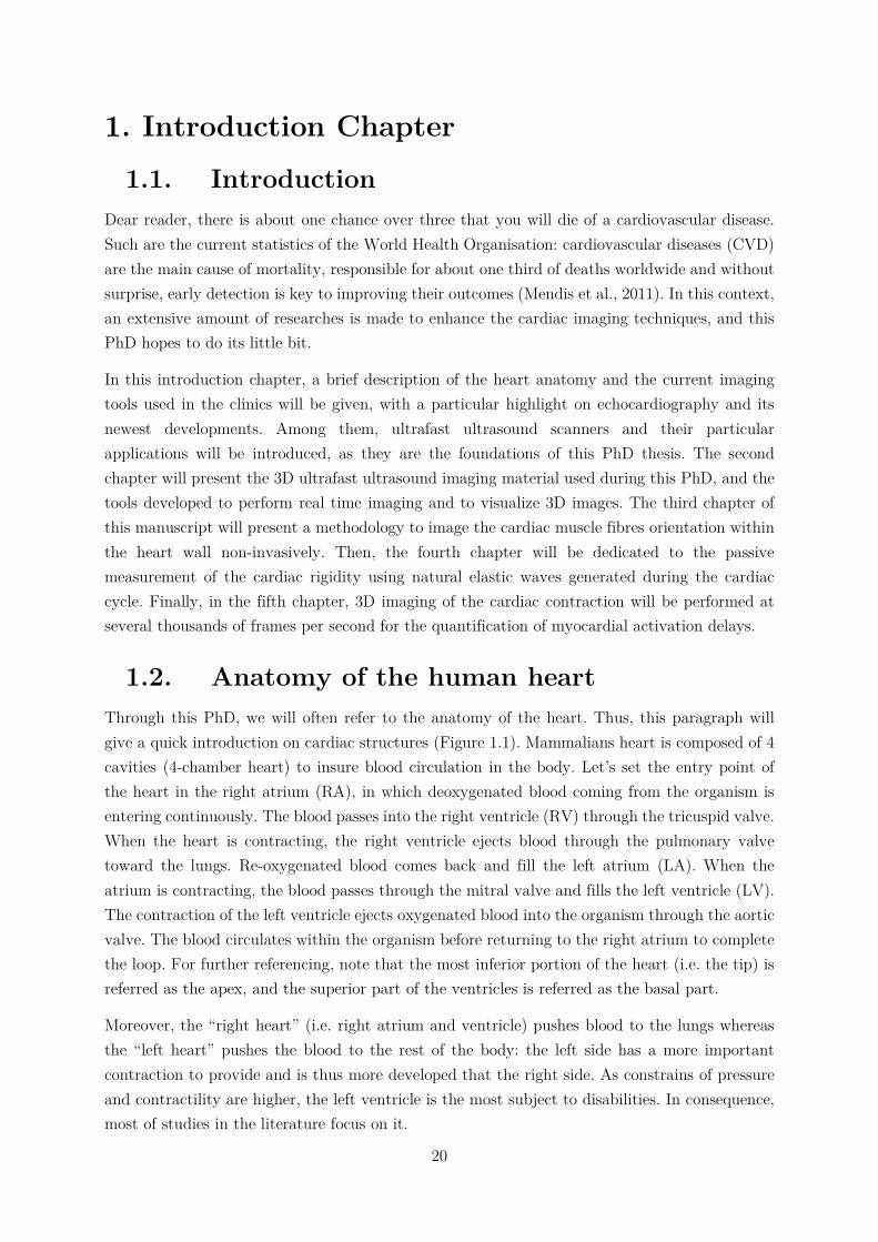
1.1. Introduction Dear reader, there is about one chance over three that you will die of a cardiovascular disease. Such are the current statistics of the World Health Organisation: cardiovascular diseases (CVD) are the main cause of mortality, responsible for about one third of deaths worldwide and without surprise, early detection is key to improving their outcomes (Mendis et al., 2011). In this context, an extensive amount of researches is made to enhance the cardiac imaging techniques, and this PhD hopes to do its little bit.

In this introduction chapter, a brief description of the heart anatomy and the current imaging tools used in the clinics will be given, with a particular highlight on echocardiography and its newest developments. Among them, ultrafast ultrasound scanners and their particular applications will be introduced, as they are the foundations of this PhD thesis. The second chapter will present the 3D ultrafast ultrasound imaging material used during this PhD, and the tools developed to perform real time imaging and to visualize 3D images. The third chapter of this manuscript will present a methodology to image the cardiac muscle fibres orientation within the heart wall non-invasively. Then, the fourth chapter will be dedicated to the passive measurement of the cardiac rigidity using natural elastic waves generated during the cardiac cycle. Finally, in the fifth chapter, 3D imaging of the cardiac contraction will be performed at several thousands of frames per second for the quantification of myocardial activation delays.

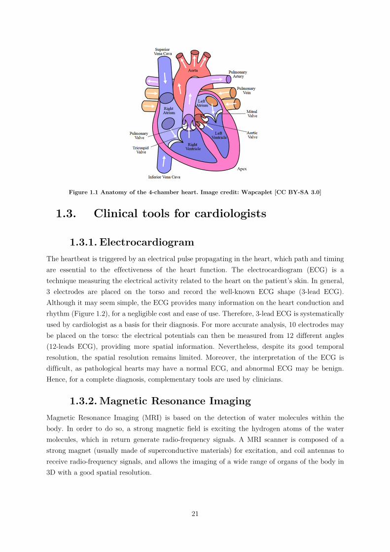
1.2. Anatomy of the human heart Through this PhD, we will often refer to the anatomy of the heart. Thus, this paragraph will give a quick introduction on cardiac structures (Figure 1.1). Mammalians heart is composed of 4 cavities (4-chamber heart) to insure blood circulation in the body. Let’s set the entry point of the heart in the right atrium (RA), in which deoxygenated blood coming from the organism is entering continuously. The blood passes into the right ventricle (RV) through the tricuspid valve. When the heart is contracting, the right ventricle ejects blood through the pulmonary valve toward the lungs. Re-oxygenated blood comes back and fill the left atrium (LA). When the atrium is contracting, the blood passes through the mitral valve and fills the left ventricle (LV). The contraction of the left ventricle ejects oxygenated blood into the organism through the aortic valve. The blood circulates within the organism before returning to the right atrium to complete the loop. For further referencing, note that the most inferior portion of the heart (i.e. the tip) is referred as the apex, and the superior part of the ventricles is referred as the basal part.

Moreover, the “right heart” (i.e. right atrium and ventricle) pushes blood to the lungs whereas the “left heart” pushes the blood to the rest of the body: the left side has a more important contraction to provide and is thus more developed that the right side. As constrains of pressure and contractility are higher, the left ventricle is the most subject to disabilities. In consequence, most of studies in the literature focus on it.

21

Figure 1.1 Anatomy of the 4-chamber heart. Image credit: Wapcaplet [CC BY-SA 3.0]

1.3. Clinical tools for cardiologists

1.3.1. Electrocardiogram The heartbeat is triggered by an electrical pulse propagating in the heart, which path and timing are essential to the effectiveness of the heart function. The electrocardiogram (ECG) is a technique measuring the electrical activity related to the heart on the patient’s skin. In general, 3 electrodes are placed on the torso and record the well-known ECG shape (3-lead ECG). Although it may seem simple, the ECG provides many information on the heart conduction and rhythm (Figure 1.2), for a negligible cost and ease of use. Therefore, 3-lead ECG is systematically used by cardiologist as a basis for their diagnosis. For more accurate analysis, 10 electrodes may be placed on the torso: the electrical potentials can then be measured from 12 different angles (12-leads ECG), providing more spatial information. Nevertheless, despite its good temporal resolution, the spatial resolution remains limited. Moreover, the interpretation of the ECG is difficult, as pathological hearts may have a normal ECG, and abnormal ECG may be benign. Hence, for a complete diagnosis, complementary tools are used by clinicians.

1.3.2. Magnetic Resonance Imaging Magnetic Resonance Imaging (MRI) is based on the detection of water molecules within the body. In order to do so, a strong magnetic field is exciting the hydrogen atoms of the water molecules, which in return generate radio-frequency signals. A MRI scanner is composed of a strong magnet (usually made of superconductive materials) for excitation, and coil antennas to receive radio-frequency signals, and allows the imaging of a wide range of organs of the body in 3D with a good spatial resolution.

22

Figure 1.2 Origins of the main ECG segments. The ECG shape is closely related to the path and timing of the electrical pulse activating the heart contraction. Figure from (Malmivuo and Plonsey,

1995)

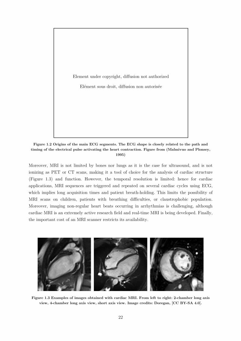
Moreover, MRI is not limited by bones nor lungs as it is the case for ultrasound, and is not ionizing as PET or CT scans, making it a tool of choice for the analysis of cardiac structure (Figure 1.3) and function. However, the temporal resolution is limited: hence for cardiac applications, MRI sequences are triggered and repeated on several cardiac cycles using ECG, which implies long acquisition times and patient breath-holding. This limits the possibility of MRI scans on children, patients with breathing difficulties, or claustrophobic population. Moreover, imaging non-regular heart beats occurring in arrhythmias is challenging, although cardiac MRI is an extremely active research field and real-time MRI is being developed. Finally, the important cost of an MRI scanner restricts its availability.

Figure 1.3 Examples of images obtained with cardiac MRI. From left to right: 2-chamber long axis view, 4-chamber long axis view, short axis view. Image credits: Doregan, [CC BY-SA 4.0].

Element under copyright, diffusion not authorized

Elément sous droit, diffusion non autorisée

23

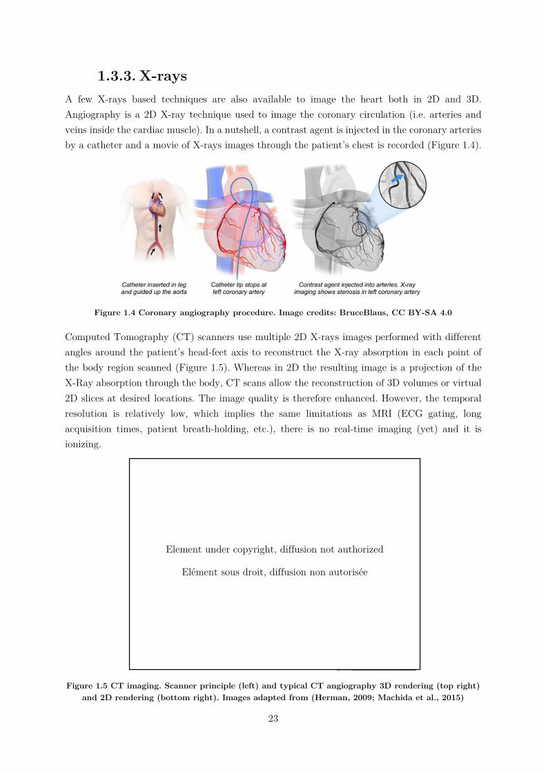
1.3.3. X-rays A few X-rays based techniques are also available to image the heart both in 2D and 3D. Angiography is a 2D X-ray technique used to image the coronary circulation (i.e. arteries and veins inside the cardiac muscle). In a nutshell, a contrast agent is injected in the coronary arteries by a catheter and a movie of X-rays images through the patient’s chest is recorded (Figure 1.4).

Figure 1.4 Coronary angiography procedure. Image credits: BruceBlaus, CC BY-SA 4.0

Computed Tomography (CT) scanners use multiple 2D X-rays images performed with different angles around the patient’s head-feet axis to reconstruct the X-ray absorption in each point of the body region scanned (Figure 1.5). Whereas in 2D the resulting image is a projection of the X-Ray absorption through the body, CT scans allow the reconstruction of 3D volumes or virtual 2D slices at desired locations. The image quality is therefore enhanced. However, the temporal resolution is relatively low, which implies the same limitations as MRI (ECG gating, long acquisition times, patient breath-holding, etc.), there is no real-time imaging (yet) and it is ionizing.

Figure 1.5 CT imaging. Scanner principle (left) and typical CT angiography 3D rendering (top right) and 2D rendering (bottom right). Images adapted from (Herman, 2009; Machida et al., 2015)



24

1.3.4. Nuclear medicine Nuclear medicine is sometimes referred as “radiology done inside out” because it records radiations emitting directly from the body rather than generated externally, such as X-rays. In order to do so, a radioactive tracer is injected in the organism and its radiations are captured by an external detector. Radiotracers are radioactive molecules bounded to carrier molecules, which can be chosen according to the purpose of the scan (tracking glucose, a particular protein, etc.). Thus, it allows the functional imaging of the organs rather than their anatomy: hence, nuclear imaging is often coupled with MRI or CT scans to obtain the anatomy of the organs.

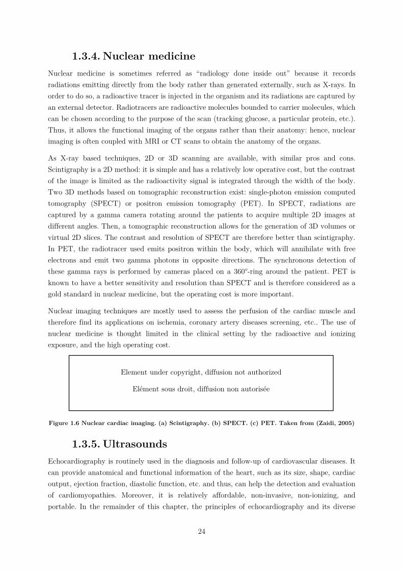
As X-ray based techniques, 2D or 3D scanning are available, with similar pros and cons. Scintigraphy is a 2D method: it is simple and has a relatively low operative cost, but the contrast of the image is limited as the radioactivity signal is integrated through the width of the body. Two 3D methods based on tomographic reconstruction exist: single-photon emission computed tomography (SPECT) or positron emission tomography (PET). In SPECT, radiations are captured by a gamma camera rotating around the patients to acquire multiple 2D images at different angles. Then, a tomographic reconstruction allows for the generation of 3D volumes or virtual 2D slices. The contrast and resolution of SPECT are therefore better than scintigraphy. In PET, the radiotracer used emits positron within the body, which will annihilate with free electrons and emit two gamma photons in opposite directions. The synchronous detection of these gamma rays is performed by cameras placed on a 360°-ring around the patient. PET is known to have a better sensitivity and resolution than SPECT and is therefore considered as a gold standard in nuclear medicine, but the operating cost is more important.

Nuclear imaging techniques are mostly used to assess the perfusion of the cardiac muscle and therefore find its applications on ischemia, coronary artery diseases screening, etc.. The use of nuclear medicine is thought limited in the clinical setting by the radioactive and ionizing exposure, and the high operating cost.

Figure 1.6 Nuclear cardiac imaging. (a) Scintigraphy. (b) SPECT. (c) PET. Taken from (Zaidi, 2005)

1.3.5. Ultrasounds Echocardiography is routinely used in the diagnosis and follow-up of cardiovascular diseases. It can provide anatomical and functional information of the heart, such as its size, shape, cardiac output, ejection fraction, diastolic function, etc. and thus, can help the detection and evaluation of cardiomyopathies. Moreover, it is relatively affordable, non-invasive, non-ionizing, and portable. In the remainder of this chapter, the principles of echocardiography and its diverse



25

modalities will be reviewed. Then, an introduction to the cutting-edge ultrasound technologies will be presented.

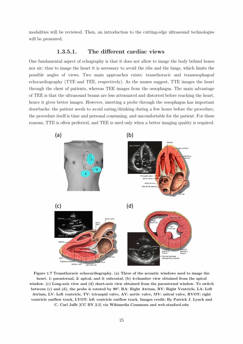
1.3.5.1. The different cardiac views One fundamental aspect of echography is that it does not allow to image the body behind bones nor air: thus to image the heart it is necessary to avoid the ribs and the lungs, which limits the possible angles of views. Two main approaches exists: transthoracic and transesophageal echocardiography (TTE and TEE, respectively). As the names suggest, TTE images the heart through the chest of patients, whereas TEE images from the oesophagus. The main advantage of TEE is that the ultrasound beams are less attenuated and distorted before reaching the heart, hence it gives better images. However, inserting a probe through the oesophagus has important drawbacks: the patient needs to avoid eating/drinking during a few hours before the procedure, the procedure itself is time and personal consuming, and uncomfortable for the patient. For these reasons, TTE is often preferred, and TEE is used only when a better imaging quality is required.

Figure 1.7 Transthoracic echocardiography. (a) Three of the acoustic windows used to image the heart. 1: parasternal, 2: apical, and 3: subcostal. (b) 4-chamber view obtained from the apical

window. (c) Long-axis view and (d) short-axis view obtained from the parasternal window. To switch between (c) and (d), the probe is rotated by 90°. RA: Right Atrium, RV: Right Ventricle, LA: Left Atrium, LV: Left ventricle, TV: tricuspid valve, AV: aortic valve, MV: mitral valve, RVOT: right ventricle outflow track, LVOT: left ventricle outflow track. Images credit: By Patrick J. Lynch and

C. Carl Jaffe [CC BY 2.5] via Wikimedia Commons and web.stanford.edu

26

In TTE, once the probe is positioned on an acoustic window (i.e. not behind bones or lungs), different views of the heart may be accessible by tilting, rotating or slightly translating the probe (Figure 1.7). For example, the apical window gives access to four different views: 2-chambers, 3-chambers, 4-chambers (Figure 1.7b) and 5-chambers views, depending on the number of structures visible. In this PhD, only transthoracic echocardiography through the apical and parasternal windows (Figure 1.7c and d) will be performed.

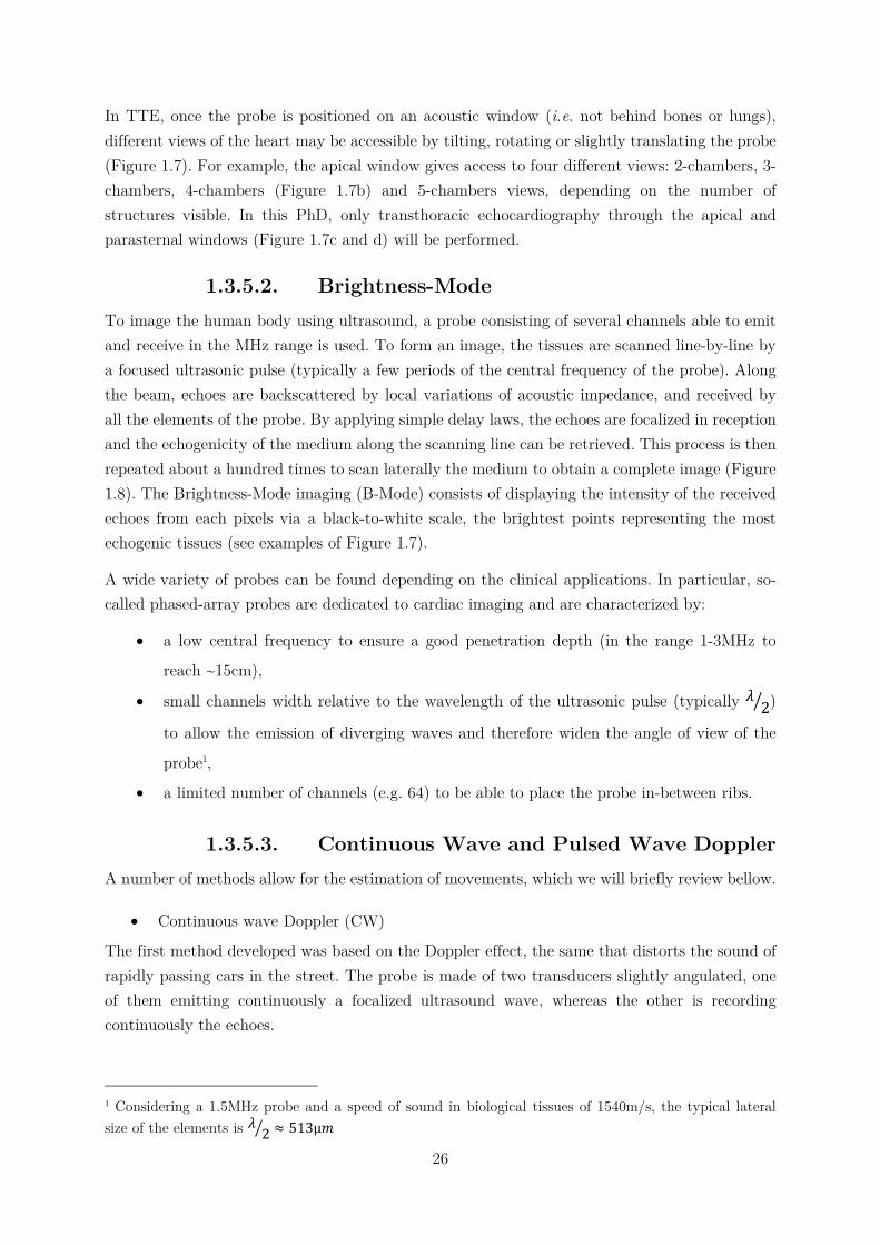
1.3.5.2. Brightness-Mode To image the human body using ultrasound, a probe consisting of several channels able to emit and receive in the MHz range is used. To form an image, the tissues are scanned line-by-line by a focused ultrasonic pulse (typically a few periods of the central frequency of the probe). Along the beam, echoes are backscattered by local variations of acoustic impedance, and received by all the elements of the probe. By applying simple delay laws, the echoes are focalized in reception and the echogenicity of the medium along the scanning line can be retrieved. This process is then repeated about a hundred times to scan laterally the medium to obtain a complete image (Figure 1.8). The Brightness-Mode imaging (B-Mode) consists of displaying the intensity of the received echoes from each pixels via a black-to-white scale, the brightest points representing the most echogenic tissues (see examples of Figure 1.7).

A wide variety of probes can be found depending on the clinical applications. In particular, so-called phased-array probes are dedicated to cardiac imaging and are characterized by:

a low central frequency to ensure a good penetration depth (in the range 1-3MHz to

reach ~15cm),

small channels width relative to the wavelength of the ultrasonic pulse (typically 𝜆2)

to allow the emission of diverging waves and therefore widen the angle of view of the

probe1,

a limited number of channels (e.g. 64) to be able to place the probe in-between ribs.

1.3.5.3. Continuous Wave and Pulsed Wave Doppler A number of methods allow for the estimation of movements, which we will briefly review bellow.

Continuous wave Doppler (CW)

The first method developed was based on the Doppler effect, the same that distorts the sound of rapidly passing cars in the street. The probe is made of two transducers slightly angulated, one of them emitting continuously a focalized ultrasound wave, whereas the other is recording continuously the echoes.

1 Considering a 1.5MHz probe and a speed of sound in biological tissues of 1540m/s, the typical lateral size of the elements is 𝜆 2 ≈ 513µ𝑚

27

Figure 1.8 Conventional echography technique. Ultrasound image formation using (a) a linear probe and (b) a cardiac probe. Image taken from (Correia, 2016)

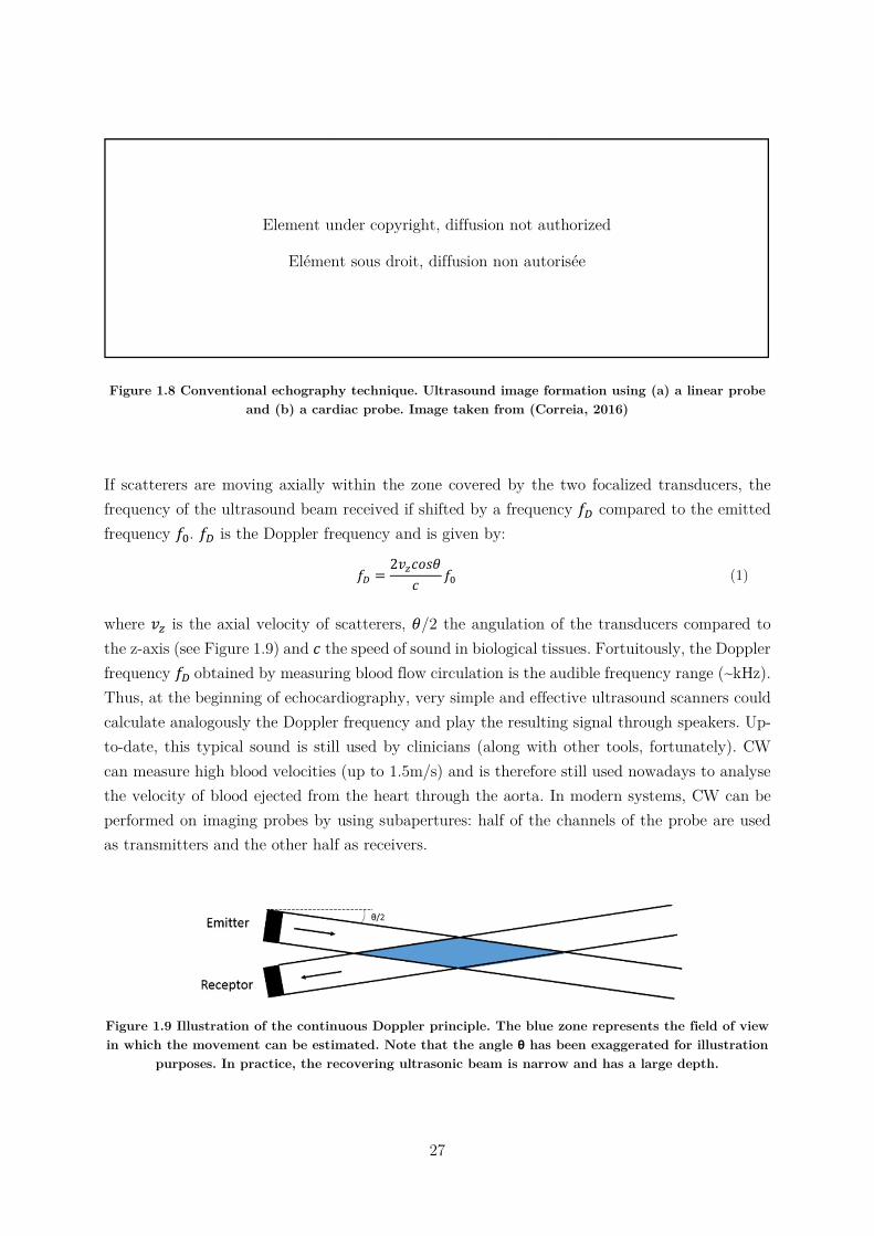
If scatterers are moving axially within the zone covered by the two focalized transducers, the frequency of the ultrasound beam received if shifted by a frequency 𝑓 compared to the emitted frequency 𝑓 . 𝑓 is the Doppler frequency and is given by:

𝑓 =2𝑣 𝑐𝑜𝑠𝜃

𝑐𝑓 (1)

where 𝑣 is the axial velocity of scatterers, 𝜃/2 the angulation of the transducers compared to the z-axis (see Figure 1.9) and 𝑐 the speed of sound in biological tissues. Fortuitously, the Doppler frequency 𝑓 obtained by measuring blood flow circulation is the audible frequency range (~kHz). Thus, at the beginning of echocardiography, very simple and effective ultrasound scanners could calculate analogously the Doppler frequency and play the resulting signal through speakers. Up-to-date, this typical sound is still used by clinicians (along with other tools, fortunately). CW can measure high blood velocities (up to 1.5m/s) and is therefore still used nowadays to analyse the velocity of blood ejected from the heart through the aorta. In modern systems, CW can be performed on imaging probes by using subapertures: half of the channels of the probe are used as transmitters and the other half as receivers.

Figure 1.9 Illustration of the continuous Doppler principle. The blue zone represents the field of view in which the movement can be estimated. Note that the angle θ has been exaggerated for illustration

purposes. In practice, the recovering ultrasonic beam is narrow and has a large depth.



28

Pulsed wave Doppler

Pulsed Wave Doppler (so-called pulsed Doppler) relies on different physics: as its name suggests, it is based on pulse-echo measurements. Focalized ultrasonic pulses are send to the medium and the echo are correlated to estimate the motion of scatterers along the beam (Baker, 1975). This method can be used with a unique transducer to provide a 1D image of movement along the beam (1D pulsed Doppler), or a linear array and thus a 2D image can be reconstructed in a similar manner as a 2D B-Mode images are made. Fortuitously, the frequency of the oscillations of the beamformed signals is related to the medium’s velocity by the same equation (1), although the mechanisms implied are different. Finally, in pulsed Doppler, a fundamental parameter is the pulse repetition frequency (PRF), as it defines the limit of velocity estimable without aliasing, according to the sampling theory: 𝑃𝑅𝐹 ≥ 2𝑓 . To work around this limitation, pulsed Doppler modes are firing several times the same scan lines of the image before sweeping to the next ones, allowing a high PRF but with a limited number of samples for each scan line. The number of transmits for each scan lines depends on the mode used, whether precise estimation in a small area or qualitative imaging in a larger area is desired. The different modes will be discussed in the following paragraphs.

Moreover, the pulsed Doppler technique described here may be applied to blood flows (Figure 1.10) or tissues motion (Figure 1.11). The latter is notably useful in echocardiography, where the estimation of motion of cardiac wall and mitral valve annulus has been investigated since the development of Doppler techniques (Isaaz et al., 1989).

To summarize, CW has the advantages of being able to measure high velocities but lacks spatial information, whereas pulsed Doppler is limited by the PRF but allows localization in space.

1.3.5.4. Visualisation of Doppler Modes Until now, we described how to estimate motion without discussing how to visualise it. Data visualisation is crucial for the effectiveness of a technique, and depends on the information to be extracted from the data, and from the nature of the data itself.

Quantitative analysis: Spectral representation

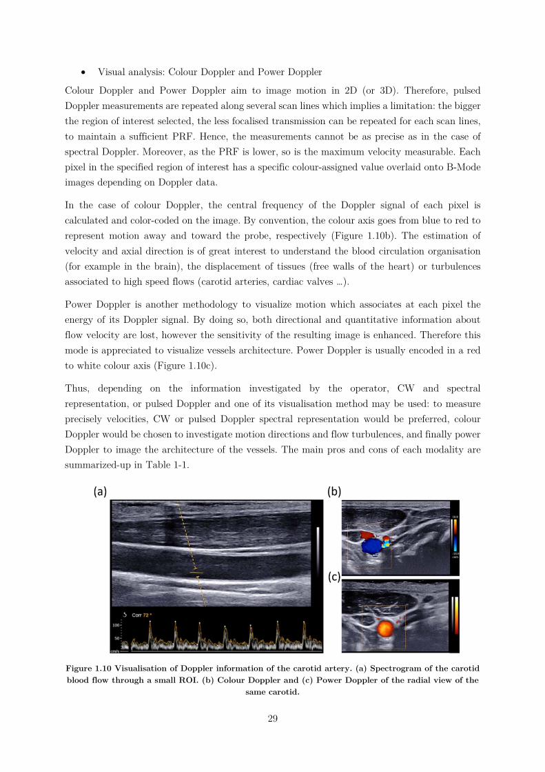
The first method to visualize motion was used on CW and pulsed Doppler and consisted of displaying a spectrogram of the Doppler signal received (Figure 1.10a). In the case of pulsed Doppler, measurements of motion are made in a few pixels wide region of interest (ROI) manually selected on the B-Mode image by the operator, and the spectrogram is calculated in these pixels. The small size of the ROI allows to repeat a high number of focalized transmissions along its scan line, improving the sampling of the Doppler signal and thus the quality of the spectrogram, but is preventing to form an image of motion. The spectrogram is the method of choice to measure blood flow velocities, as well as cardiac synchronisation (e.g. delay between peak velocities across the different valves). Note that this technique is often referred as “pulsed-Doppler” itself; to avoid this ambiguity, we will refer to it as “spectral” Doppler in this document.

29

Visual analysis: Colour Doppler and Power Doppler

Colour Doppler and Power Doppler aim to image motion in 2D (or 3D). Therefore, pulsed Doppler measurements are repeated along several scan lines which implies a limitation: the bigger the region of interest selected, the less focalised transmission can be repeated for each scan lines, to maintain a sufficient PRF. Hence, the measurements cannot be as precise as in the case of spectral Doppler. Moreover, as the PRF is lower, so is the maximum velocity measurable. Each pixel in the specified region of interest has a specific colour-assigned value overlaid onto B-Mode images depending on Doppler data.

In the case of colour Doppler, the central frequency of the Doppler signal of each pixel is calculated and color-coded on the image. By convention, the colour axis goes from blue to red to represent motion away and toward the probe, respectively (Figure 1.10b). The estimation of velocity and axial direction is of great interest to understand the blood circulation organisation (for example in the brain), the displacement of tissues (free walls of the heart) or turbulences associated to high speed flows (carotid arteries, cardiac valves …).

Power Doppler is another methodology to visualize motion which associates at each pixel the energy of its Doppler signal. By doing so, both directional and quantitative information about flow velocity are lost, however the sensitivity of the resulting image is enhanced. Therefore this mode is appreciated to visualize vessels architecture. Power Doppler is usually encoded in a red to white colour axis (Figure 1.10c).

Thus, depending on the information investigated by the operator, CW and spectral representation, or pulsed Doppler and one of its visualisation method may be used: to measure precisely velocities, CW or pulsed Doppler spectral representation would be preferred, colour Doppler would be chosen to investigate motion directions and flow turbulences, and finally power Doppler to image the architecture of the vessels. The main pros and cons of each modality are summarized-up in Table 1-1.

Figure 1.10 Visualisation of Doppler information of the carotid artery. (a) Spectrogram of the carotid blood flow through a small ROI. (b) Colour Doppler and (c) Power Doppler of the radial view of the

same carotid.

30

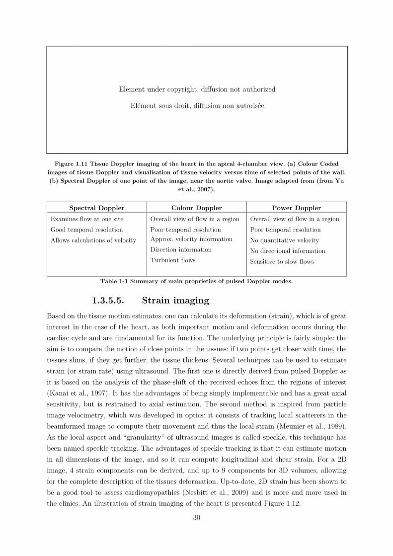
Figure 1.11 Tissue Doppler imaging of the heart in the apical 4-chamber view. (a) Colour Coded images of tissue Doppler and visualisation of tissue velocity versus time of selected points of the wall. (b) Spectral Doppler of one point of the image, near the aortic valve. Image adapted from (from Yu

et al., 2007).

Spectral Doppler Colour Doppler Power Doppler Examines flow at one site Good temporal resolution Allows calculations of velocity

Overall view of flow in a region Poor temporal resolution Approx. velocity information Direction information Turbulent flows

Overall view of flow in a region Poor temporal resolution No quantitative velocity No directional information Sensitive to slow flows

Table 1-1 Summary of main proprieties of pulsed Doppler modes.

1.3.5.5. Strain imaging Based on the tissue motion estimates, one can calculate its deformation (strain), which is of great interest in the case of the heart, as both important motion and deformation occurs during the cardiac cycle and are fundamental for its function. The underlying principle is fairly simple: the aim is to compare the motion of close points in the tissues: if two points get closer with time, the tissues slims, if they get further, the tissue thickens. Several techniques can be used to estimate strain (or strain rate) using ultrasound. The first one is directly derived from pulsed Doppler as it is based on the analysis of the phase-shift of the received echoes from the regions of interest (Kanai et al., 1997). It has the advantages of being simply implementable and has a great axial sensitivity, but is restrained to axial estimation. The second method is inspired from particle image velocimetry, which was developed in optics: it consists of tracking local scatterers in the beamformed image to compute their movement and thus the local strain (Meunier et al., 1989). As the local aspect and “granularity” of ultrasound images is called speckle, this technique has been named speckle tracking. The advantages of speckle tracking is that it can estimate motion in all dimensions of the image, and so it can compute longitudinal and shear strain. For a 2D image, 4 strain components can be derived, and up to 9 components for 3D volumes, allowing for the complete description of the tissues deformation. Up-to-date, 2D strain has been shown to be a good tool to assess cardiomyopathies (Nesbitt et al., 2009) and is more and more used in the clinics. An illustration of strain imaging of the heart is presented Figure 1.12.



31

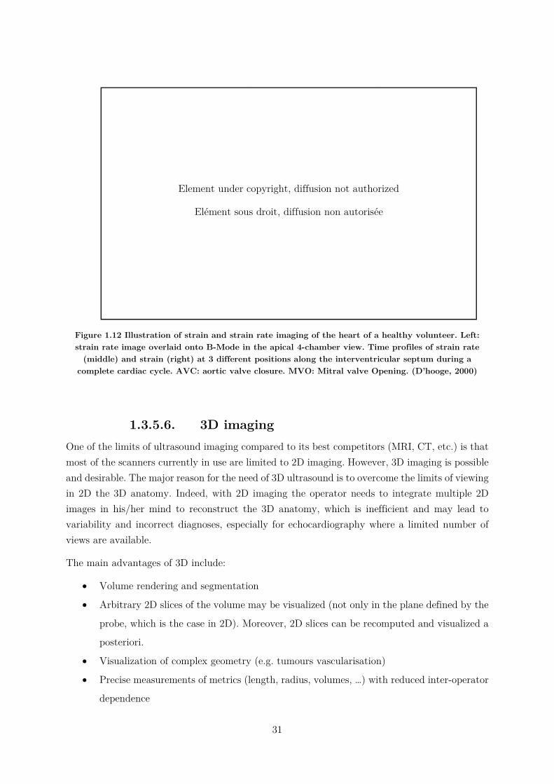
Figure 1.12 Illustration of strain and strain rate imaging of the heart of a healthy volunteer. Left: strain rate image overlaid onto B-Mode in the apical 4-chamber view. Time profiles of strain rate

(middle) and strain (right) at 3 different positions along the interventricular septum during a complete cardiac cycle. AVC: aortic valve closure. MVO: Mitral valve Opening. (D’hooge, 2000)

1.3.5.6. 3D imaging One of the limits of ultrasound imaging compared to its best competitors (MRI, CT, etc.) is that most of the scanners currently in use are limited to 2D imaging. However, 3D imaging is possible and desirable. The major reason for the need of 3D ultrasound is to overcome the limits of viewing in 2D the 3D anatomy. Indeed, with 2D imaging the operator needs to integrate multiple 2D images in his/her mind to reconstruct the 3D anatomy, which is inefficient and may lead to variability and incorrect diagnoses, especially for echocardiography where a limited number of views are available.

The main advantages of 3D include:

Volume rendering and segmentation

Arbitrary 2D slices of the volume may be visualized (not only in the plane defined by the

probe, which is the case in 2D). Moreover, 2D slices can be recomputed and visualized a

posteriori.

Visualization of complex geometry (e.g. tumours vascularisation)

Precise measurements of metrics (length, radius, volumes, …) with reduced inter-operator

dependence



32

Up-to-date, two main techniques exist to perform 3D ultrasound imaging: moving a 2D transducer to obtain multiple 2D images, or using a dedicated 3D matrix probe. The former case can again be divided into subcategories, depending on the way the 2D images through the volume are obtained: one possibility is to scan freely move the probe on the patient’s skin and recombine the images using correlation algorithms (Downey and Fenster, 1995). In this case, some systems may integrate a tracking device to register the movement of the probe (Mercier et al., 2005). The other subcategory consists of building a “virtual” 3D probe consisting of a linear array that can be either translated, rotated or tilted by a motor to scan the volume. Finally, in the second main technique a dedicated 3D probe composed of a 2D matrix of ultrasonic transducers is used, allowing to directly image the volume below the probe. In a similar manner than with phased-array probes, diverging waves can be emitted to extend the field of view to a pyramidal shape. This solution implies a high number of transducers: to be used with standard ultrasound scanners, electronics are integrated within the probe to pre-process the signals and reduced the number of channels to be sampled. Once 3D volumes acquired, the 2D techniques detailed above can be directly applied to obtain volumetric Doppler, strain imaging, etc..

Studies have shown the potential of 3D ultrasound imaging for cardiac applications on foetuses and adults hearts, but it is however still limited by the low framerate (Lang et al., 2012; Yagel et al., 2007).

1.3.6. Current limits of clinical tools Although the large number of tools available to clinicians to examine the heart, each of them has drawbacks and limitations. An ideal imaging tool would be: cheap, non-ionizing nor invasive, 3D and with a good temporal resolution.

1.4. Ultrafast ultrasound imaging

1.4.1. Plane waves, diverging waves and coherent

compounding In the following paragraphs, we will present ultrafast ultrasound imaging, to be opposed to conventional ultrasound. In the latter, we saw that an image is formed line by line, so the maximum framerate is limited by the necessary time to form one line (i.e., the depth of the image) multiplied by number of desired lines. Ultrafast imaging relies on the insonification of the whole region to be scanned in one ultrasound transmission. Therefore, the time to form an image is only limited by the time-of-flight necessary for the wave to travel back and forth the depth of the image. If the desired image has N=100 lines, ultrafast imaging allows to multiply the framerate by a factor N=100, allowing to reach up to 10.000 frames/seconds. For linear array probes, a plane wave is transmitted to scan the medium directly below the probe, whereas

33

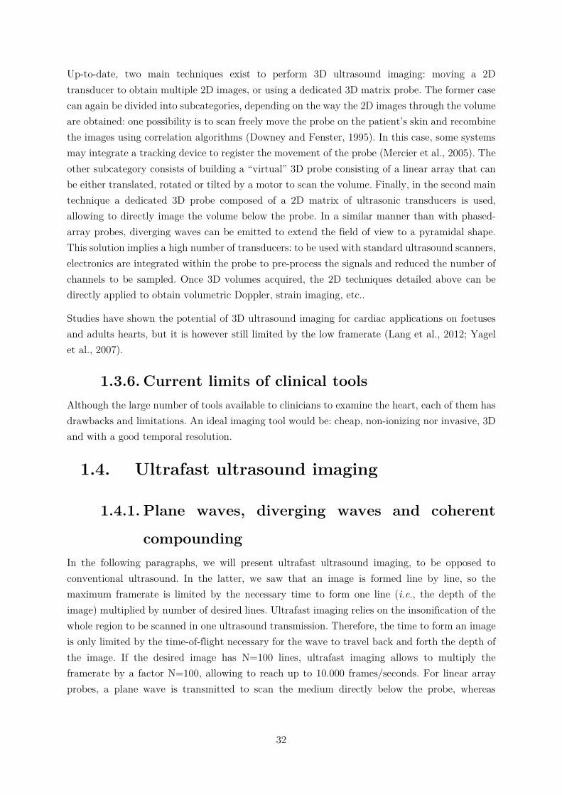
diverging waves can be sent by phased-array probes to image a wider sector2 (Figure 1.13). To form the image, the echoes are processed by a conventional delay-and-sum beamformer. The drawback of ultrafast imaging is that as the transmitted beam is not focalized, the contrast and the resolution of the resulting image is lower than what is obtained with conventional ultrasound imaging.

Figure 1.13 Principle of ultrafast ultrasound imaging. The whole medium is insonified by only one ultrasound pulse. The wave sent by the transducer can be plane for linear probes (a) or diverging for

phased-array probes (b). Figure from (Correia, 2016).

To overcome these limits, Montaldo et al., suggested the transmission of multiple tilted plane waves. Their coherent compounding in post-processing is equivalent to synthetic focusing in emission, as illustrated on Figure 1.14 (under the assumption that there is no significant movement in between their transmissions, as we will discussed later in chapter 3). By doing so, both contrast and resolution can be enhanced and compared to conventional ultrasound imaging, while the framerate is still significantly higher (Montaldo et al., 2009). As always, a trade-off has to be made: the higher the number of plane waves used, the better the synthetic focusing and hence the resulting image, but the lower the framerate. Thus, the choice of the number of plane waves is made according to the experimental requirements: typically, about 40 plane waves are sufficient to retrieve a quality equivalent to conventional ultrasound.

That being said, one could legitimately wonder the point of generating real time images at thousands of frames per seconds. Thus in the following paragraphs, we will introduce some applications made possible by ultrafast ultrasound imaging.

2 Note that for the sake of simplicity, we will refer to plane waves to further describe this technology in this manuscript, but all the developments can be applied on diverging waves too.



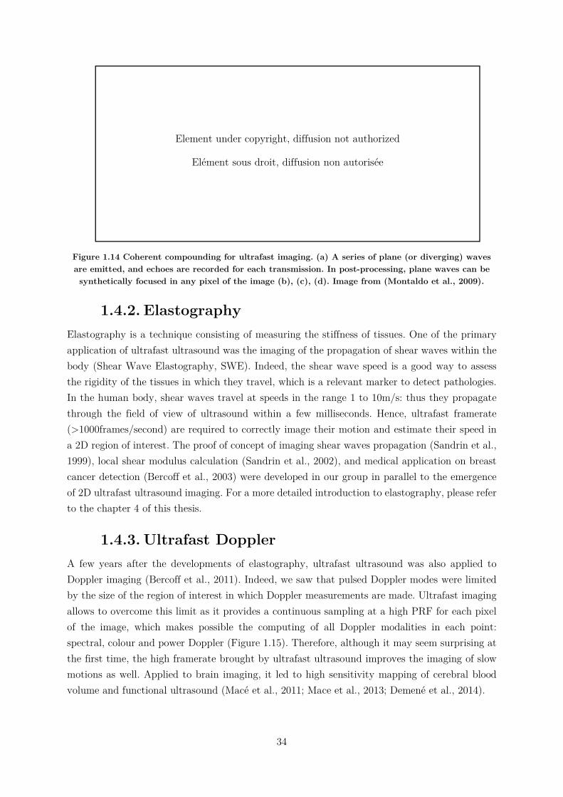
34

Figure 1.14 Coherent compounding for ultrafast imaging. (a) A series of plane (or diverging) waves are emitted, and echoes are recorded for each transmission. In post-processing, plane waves can be synthetically focused in any pixel of the image (b), (c), (d). Image from (Montaldo et al., 2009).

1.4.2. Elastography Elastography is a technique consisting of measuring the stiffness of tissues. One of the primary application of ultrafast ultrasound was the imaging of the propagation of shear waves within the body (Shear Wave Elastography, SWE). Indeed, the shear wave speed is a good way to assess the rigidity of the tissues in which they travel, which is a relevant marker to detect pathologies. In the human body, shear waves travel at speeds in the range 1 to 10m/s: thus they propagate through the field of view of ultrasound within a few milliseconds. Hence, ultrafast framerate (>1000frames/second) are required to correctly image their motion and estimate their speed in a 2D region of interest. The proof of concept of imaging shear waves propagation (Sandrin et al., 1999), local shear modulus calculation (Sandrin et al., 2002), and medical application on breast cancer detection (Bercoff et al., 2003) were developed in our group in parallel to the emergence of 2D ultrafast ultrasound imaging. For a more detailed introduction to elastography, please refer to the chapter 4 of this thesis.

1.4.3. Ultrafast Doppler A few years after the developments of elastography, ultrafast ultrasound was also applied to Doppler imaging (Bercoff et al., 2011). Indeed, we saw that pulsed Doppler modes were limited by the size of the region of interest in which Doppler measurements are made. Ultrafast imaging allows to overcome this limit as it provides a continuous sampling at a high PRF for each pixel of the image, which makes possible the computing of all Doppler modalities in each point: spectral, colour and power Doppler (Figure 1.15). Therefore, although it may seem surprising at the first time, the high framerate brought by ultrafast ultrasound improves the imaging of slow motions as well. Applied to brain imaging, it led to high sensitivity mapping of cerebral blood volume and functional ultrasound (Macé et al., 2011; Mace et al., 2013; Demené et al., 2014).



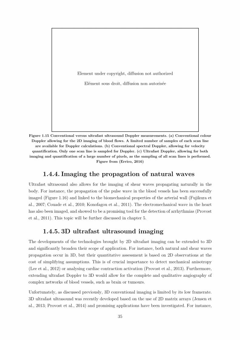
35

Figure 1.15 Conventional versus ultrafast ultrasound Doppler measurements. (a) Conventional colour Doppler allowing for the 2D imaging of blood flows. A limited number of samples of each scan line

are available for Doppler calculations. (b) Conventional spectral Doppler, allowing for velocity quantification. Only one scan line is sampled for Doppler. (c) Ultrafast Doppler, allowing for both

imaging and quantification of a large number of pixels, as the sampling of all scan lines is performed. Figure from (Errico, 2016)

1.4.4. Imaging the propagation of natural waves Ultrafast ultrasound also allows for the imaging of shear waves propagating naturally in the body. For instance, the propagation of the pulse wave in the blood vessels has been successfully imaged (Figure 1.16) and linked to the biomechanical properties of the arterial wall (Fujikura et al., 2007; Couade et al., 2010; Konofagou et al., 2011). The electromechanical wave in the heart has also been imaged, and showed to be a promising tool for the detection of arrhythmias (Provost et al., 2011). This topic will be further discussed in chapter 5.

1.4.5. 3D ultrafast ultrasound imaging The developments of the technologies brought by 2D ultrafast imaging can be extended to 3D and significantly broaden their scope of application. For instance, both natural and shear waves propagation occur in 3D, but their quantitative assessment is based on 2D observations at the cost of simplifying assumptions. This is of crucial importance to detect mechanical anisotropy (Lee et al., 2012) or analysing cardiac contraction activation (Provost et al., 2013). Furthermore, extending ultrafast Doppler to 3D would allow for the complete and qualitative angiography of complex networks of blood vessels, such as brain or tumours.

Unfortunately, as discussed previously, 3D conventional imaging is limited by its low framerate. 3D ultrafast ultrasound was recently developed based on the use of 2D matrix arrays (Jensen et al., 2013; Provost et al., 2014) and promising applications have been investigated. For instance,



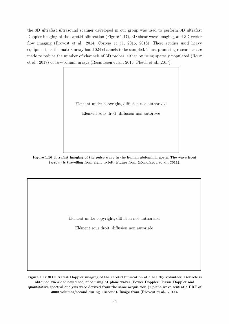
36

the 3D ultrafast ultrasound scanner developed in our group was used to perform 3D ultrafast Doppler imaging of the carotid bifurcation (Figure 1.17), 3D shear wave imaging, and 3D vector flow imaging (Provost et al., 2014; Correia et al., 2016, 2018). These studies used heavy equipment, as the matrix array had 1024 channels to be sampled. Thus, promising researches are made to reduce the number of channels of 3D probes, either by using sparsely populated (Roux et al., 2017) or row-column arrays (Rasmussen et al., 2015; Flesch et al., 2017).

Figure 1.16 Ultrafast imaging of the pulse wave in the human abdominal aorta. The wave front (arrow) is travelling from right to left. Figure from (Konofagou et al., 2011).

Figure 1.17 3D ultrafast Doppler imaging of the carotid bifurcation of a healthy volunteer. B-Mode is obtained via a dedicated sequence using 81 plane waves. Power Doppler, Tissue Doppler and

quantitative spectral analysis were derived from the same acquisition (1 plane wave sent at a PRF of 3000 volumes/second during 1 second). Image from (Provost et al., 2014).





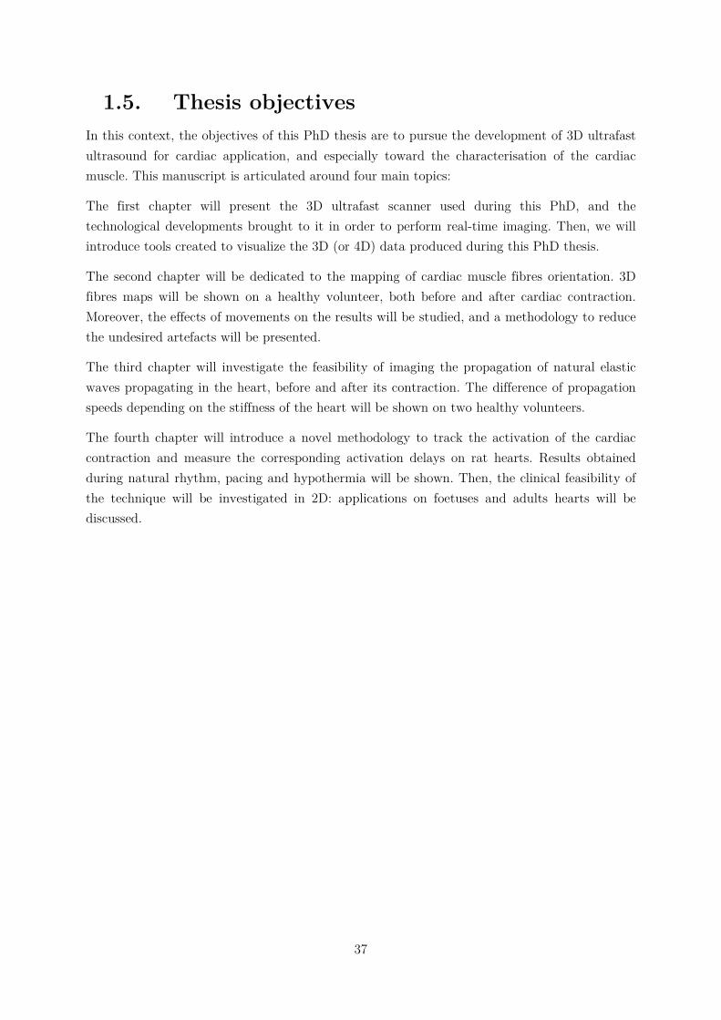
37

1.5. Thesis objectives In this context, the objectives of this PhD thesis are to pursue the development of 3D ultrafast ultrasound for cardiac application, and especially toward the characterisation of the cardiac muscle. This manuscript is articulated around four main topics:

The first chapter will present the 3D ultrafast scanner used during this PhD, and the technological developments brought to it in order to perform real-time imaging. Then, we will introduce tools created to visualize the 3D (or 4D) data produced during this PhD thesis.

The second chapter will be dedicated to the mapping of cardiac muscle fibres orientation. 3D fibres maps will be shown on a healthy volunteer, both before and after cardiac contraction. Moreover, the effects of movements on the results will be studied, and a methodology to reduce the undesired artefacts will be presented.

The third chapter will investigate the feasibility of imaging the propagation of natural elastic waves propagating in the heart, before and after its contraction. The difference of propagation speeds depending on the stiffness of the heart will be shown on two healthy volunteers.

The fourth chapter will introduce a novel methodology to track the activation of the cardiac contraction and measure the corresponding activation delays on rat hearts. Results obtained during natural rhythm, pacing and hypothermia will be shown. Then, the clinical feasibility of the technique will be investigated in 2D: applications on foetuses and adults hearts will be discussed.

38

1.6. Chapter bibliography

Baker, D.W., 1975. Pulsed ultrasonic Doppler blood-flow sensing. IEEE SU 17, 170–185.

Bercoff, J., Chaffai, S., Tanter, M., Sandrin, L., Catheline, S., Fink, M., Gennisson, J.L., Meunier, M., 2003. In vivo breast tumor detection using transient elastography. Ultrasound in Medicine & Biology 29, 1387–1396. https://doi.org/10.1016/S0301-5629(03)00978-5

Bercoff, J., Montaldo, G., Loupas, T., Savery, D., Mézière, F., Fink, M., Tanter, M., 2011. Ultrafast compound doppler imaging: providing full blood flow characterization. IEEE Transactions on Ultrasonics, Ferroelectrics and Frequency Control 58, 134–147. https://doi.org/10.1109/TUFFC.2011.1780

Correia, M., Deffieux, T., Chatelin, S., Provost, J., Tanter, M., Pernot, M., 2018. 3D elastic tensor imaging in weakly transversely isotropic soft tissues. Physics in Medicine & Biology 63, 155005. https://doi.org/10.1088/1361-6560/aacfaf

Correia, M., Provost, J., Tanter, M., Pernot, M., 2016. 4D ultrafast ultrasound flow imaging: in vivo quantification of arterial volumetric flow rate in a single heartbeat. Physics in Medicine and Biology 61, L48–L61. https://doi.org/10.1088/0031-9155/61/23/L48

Correia, M.F.R., 2016. From 2D to 3D cardiovascular ultrafast ultrasound imaging : new insights in shear wave elastography and blood flow imaging.

Couade, M., Pernot, M., Prada, C., Messas, E., Emmerich, J., Bruneval, P., Criton, A., Fink, M., Tanter, M., 2010. Quantitative Assessment of Arterial Wall Biomechanical Properties Using Shear Wave Imaging. Ultrasound in Medicine & Biology 36, 1662–1676. https://doi.org/10.1016/j.ultrasmedbio.2010.07.004

Delannoy, B., Torguet, R., Bruneel, C., Bridoux, E., 1979. Ultrafast Electronical Image Reconstruction Device, in: Lancée, C.T. (Ed.), Echocardiology. Springer Netherlands, Dordrecht, pp. 447–450. https://doi.org/10.1007/978-94-009-9324-2_62

Demené, C., Pernot, M., Biran, V., Alison, M., Fink, M., Baud, O., Tanter, M., 2014. Ultrafast Doppler Reveals the Mapping of Cerebral Vascular Resistivity in Neonates. Journal of Cerebral Blood Flow & Metabolism 34, 1009–1017. https://doi.org/10.1038/jcbfm.2014.49

D’hooge, J., 2000. Regional Strain and Strain Rate Measurements by Cardiac Ultrasound: Principles, Implementation and Limitations. European Journal of Echocardiography 1, 154–170. https://doi.org/10.1053/euje.2000.0031

Downey, D.B., Fenster, A., 1995. Vascular imaging with a three-dimensional power Doppler system. American Journal of Roentgenology 165, 665–668. https://doi.org/10.2214/ajr.165.3.7645492

39

Errico, C., 2016. Ultrasound sensitive agents for transcranial functional imaging, super-resolution microscopy and drug delivery.

Flesch, M., Pernot, M., Provost, J., Ferin, G., Nguyen-Dinh, A., Tanter, M., Deffieux, T., 2017. 4D in vivo ultrafast ultrasound imaging using a row-column addressed matrix and coherently-compounded orthogonal plane waves. Phys. Med. Biol. 62, 4571. https://doi.org/10.1088/1361-6560/aa63d9

Fujikura, K., Luo, J., Gamarnik, V., Pernot, M., Fukumoto, R., Tilson, M.D., Konofagou, E.E., 2007. A Novel Noninvasive Technique for Pulse-Wave Imaging and Characterization of Clinically-Significant Vascular Mechanical Properties In Vivo. Ultrasonic Imaging 29, 137–154. https://doi.org/10.1177/016173460702900301

Herman, G.T., 2009. Fundamentals of Computerized Tomography: Image Reconstruction from Projections. Springer Science & Business Media.

Isaaz, K., Thompson, A., Ethevenot, G., Cloez, J.L., Brembilla, B., Pernot, C., 1989. Doppler echocardiographic measurement of low velocity motion of the left ventricular posterior wall. The American Journal of Cardiology 64, 66–75. https://doi.org/10.1016/0002-9149(89)90655-3

Jensen, J.A., Holten-Lund, H., Nilsson, R.T., Hansen, M., Larsen, U.D., Domsten, R.P., Tomov, B.G., Stuart, M.B., Nikolov, S.I., Pihl, M.J., Yigang Du, Rasmussen, J.H., Rasmussen, M.F., 2013. SARUS: A synthetic aperture real-time ultrasound system. IEEE Transactions on Ultrasonics, Ferroelectrics, and Frequency Control 60, 1838–1852. https://doi.org/10.1109/TUFFC.2013.2770

Kanai, H., Hasegawa, H., Chubachi, N., Koiwa, Y., Tanaka, M., 1997. Noninvasive evaluation of local myocardial thickening and its color-coded imaging. IEEE Transactions on Ultrasonics, Ferroelectrics and Frequency Control 44, 752–768. https://doi.org/10.1109/58.655190

Konofagou, E., Lee, W.-N., Luo, J., Provost, J., Vappou, J., 2011. Physiologic Cardiovascular Strain and Intrinsic Wave Imaging. Annual Review of Biomedical Engineering 13, 477–505. https://doi.org/10.1146/annurev-bioeng-071910-124721

Lang, R.M., Badano, L.P., Tsang, W., Adams, D.H., Agricola, E., Buck, T., Faletra, F.F., Franke, A., Hung, J., de Isla, L.P., Kamp, O., Kasprzak, J.D., Lancellotti, P., Marwick, T.H., McCulloch, M.L., Monaghan, M.J., Nihoyannopoulos, P., Pandian, N.G., Pellikka, P.A., Pepi, M., Roberson, D.A., Shernan, S.K., Shirali, G.S., Sugeng, L., Ten Cate, F.J., Vannan, M.A., Zamorano, J.L., Zoghbi, W.A., 2012. EAE/ASE Recommendations for Image Acquisition and Display Using Three-Dimensional Echocardiography. European Heart Journal - Cardiovascular Imaging 13, 1–46. https://doi.org/10.1093/ehjci/jer316

Macé, E., Montaldo, G., Cohen, I., Baulac, M., Fink, M., Tanter, M., 2011. Functional ultrasound imaging of the brain. Nature Methods 8, 662–664. https://doi.org/10.1038/nmeth.1641

40

Mace, E., Montaldo, G., Osmanski, B.-F., Cohen, I., Fink, M., Tanter, M., 2013. Functional ultrasound imaging of the brain: theory and basic principles. IEEE Transactions on Ultrasonics, Ferroelectrics and Frequency Control 60, 492–506. https://doi.org/10.1109/TUFFC.2013.2592

Machida, H., Tanaka, I., Fukui, R., Shen, Y., Ishikawa, T., Tate, E., Ueno, E., 2015. Current and Novel Imaging Techniques in Coronary CT. RadioGraphics 35, 991–1010. https://doi.org/10.1148/rg.2015140181

Malmivuo, J., Plonsey, R., 1995. BioelectromagnetismPrinciples and Applications of Bioelectric and Biomagnetic Fields. Oxford University Press. https://doi.org/10.1093/acprof:oso/9780195058239.001.0001

Mendis, S., Puska, P., Norrving, B., World Health Organization, World Heart Federation, World Stroke Organization (Eds.), 2011. Global atlas on cardiovascular disease prevention and control. World Health Organization in collaboration with the World Heart Federation and the World Stroke Organization, Geneva.

Mercier, L., Langø, T., Lindseth, F., Collins, L.D., 2005. A review of calibration techniques for freehand 3-D ultrasound systems. Ultrasound in Medicine & Biology 31, 143–165. https://doi.org/10.1016/j.ultrasmedbio.2004.11.001

Meunier, J., Bertrand, M., Mailloux, G.E., Petitclerc, R., 1989. Local myocardial deformation computed from speckle motion, in: Proceedings. Computers in Cardiology 1988. Presented at the Proceedings. Computers in Cardiology 1988, IEEE Comput. Soc. Press, Washington, DC, USA, pp. 133–136. https://doi.org/10.1109/CIC.1988.72583

Montaldo, G., Tanter, M., Bercoff, J., Benech, N., Fink, M., 2009. Coherent plane-wave compounding for very high frame rate ultrasonography and transient elastography. IEEE Transactions on Ultrasonics, Ferroelectrics and Frequency Control 56, 489–506. https://doi.org/10.1109/TUFFC.2009.1067

Nesbitt, G.C., Mankad, S., Oh, J.K., 2009. Strain imaging in echocardiography: methods and clinical applications. The International Journal of Cardiovascular Imaging 25, 9–22. https://doi.org/10.1007/s10554-008-9414-1

Provost, J., Gambhir, A., Vest, J., Garan, H., Konofagou, E.E., 2013. A clinical feasibility study of atrial and ventricular electromechanical wave imaging. Heart Rhythm 10, 856–862. https://doi.org/10.1016/j.hrthm.2013.02.028

Provost, J., Lee, W.-N., Fujikura, K., Konofagou, E.E., 2011. Imaging the electromechanical activity of the heart in vivo. Proceedings of the National Academy of Sciences 108, 8565–8570.

Provost, J., Papadacci, C., Arango, J.E., Imbault, M., Fink, M., Gennisson, J.-L., Tanter, M., Pernot, M., 2014. 3D ultrafast ultrasound imaging in vivo. Physics in Medicine and Biology 59, L1–L13. https://doi.org/10.1088/0031-9155/59/19/L1

41

Rasmussen, M.F., Christiansen, T.L., Thomsen, E.V., Jensen, J.A., 2015. 3-D imaging using row-column-addressed arrays with integrated apodization - part i: apodization design and line element beamforming. IEEE Transactions on Ultrasonics, Ferroelectrics, and Frequency Control 62, 947–958. https://doi.org/10.1109/TUFFC.2014.006531

Roux, E., Ramalli, A., Liebgott, H., Cachard, C., Robini, M.C., Tortoli, P., 2017. Wideband 2-D Array Design Optimization With Fabrication Constraints for 3-D US Imaging. IEEE Transactions on Ultrasonics, Ferroelectrics, and Frequency Control 64, 108–125. https://doi.org/10.1109/TUFFC.2016.2614776

Sandrin, L., Catheline, S., Tanter, M., Hennequin, X., Fink, M., 1999. Time-Resolved Pulsed Elastography with Ultrafast Ultrasonic Imaging , Time-Resolved Pulsed Elastography with Ultrafast Ultrasonic Imaging. Ultrason Imaging 21, 259–272. https://doi.org/10.1177/016173469902100402

Sandrin, L., Tanter, M., Catheline, S., Fink, M., 2002. Shear modulus imaging with 2-D transient elastography. IEEE Transactions on Ultrasonics, Ferroelectrics and Frequency Control 49, 426–435. https://doi.org/10.1109/58.996560

Wei-Ning Lee, Pernot, M., Couade, M., Messas, E., Bruneval, P., Bel, A., Hagege, A.A., Fink, M., Tanter, M., 2012. Mapping Myocardial Fiber Orientation Using Echocardiography-Based Shear Wave Imaging. IEEE Transactions on Medical Imaging 31, 554–562. https://doi.org/10.1109/TMI.2011.2172690

Yagel, S., Cohen, S.M., Shapiro, I., Valsky, D.V., 2007. 3D and 4D ultrasound in fetal cardiac scanning: a new look at the fetal heart. Ultrasound in Obstetrics & Gynecology 29, 81–95. https://doi.org/10.1002/uog.3912

Yu, C.-M., Sanderson, J.E., Marwick, T.H., Oh, J.K., 2007. Tissue Doppler Imaging. Journal of the American College of Cardiology 49, 1903–1914. https://doi.org/10.1016/j.jacc.2007.01.078

Zaidi, H. (Ed.), 2005. Quantum analysis in nuclear medicine imaging. Springer, New York, NY.

43

: 3D Ultrafast Ultrasound

Imaging

2. : 3D Ultrafast Ultrasound Imaging ..................................................................................... 43

2.1. Introduction ................................................................................................................. 44

2.2. Presentation of the 3D ultrafast ultrasound scanners and probes ............................... 45

2.3. Development of specific tools ...................................................................................... 47

2.3.1. Real-time imaging ................................................................................................ 47

2.3.1.1. Saddle imaging: 2D imaging with a 3D probe .............................................. 47

2.3.1.2. Parallel processing ........................................................................................ 49

2.3.1.3. Triggering acquisitions .................................................................................. 50

2.3.2. Visualisation tools ................................................................................................ 50

2.3.2.1. Fibres ............................................................................................................ 51

2.3.2.2. Heart walls .................................................................................................... 51

2.3.2.3. The 4th dimension ......................................................................................... 51

2.4. Conclusion ................................................................................................................... 51


44

3D Ultrafast Ultrasound Imaging

2.1. Introduction 3D ultrasound imaging is of great interest as it would overcome the 2D-limitations of echography, but yet conventional ultrasound methodology does not allow to perform 3D imaging with sufficient frame rates for cardiac applications (Yagel et al., 2007; Lang et al., 2012). However, over the last few years, 2D ultrasound imaging has undergone important developments with the introduction of ultrafast imaging techniques achieving up to 10.000 frames/s, as opposed to 50 to 200 frames/s in traditional clinical systems. Several methods exists to reach ultrafast frame rates in large fields of view: multiline transmissions (Mallart and Fink, 1992; Tong et al., 2013, 2014), plane waves transmission (Sandrin et al., 1999; Tanter et al., 2002), diverging waves (Couade et al., 2009; Honjo et al., 2010; Provost et al., 2011b; Papadacci et al., 2014), or retrospective gating techniques (Pernot et al., 2007; Shougang Wang et al., 2008; Provost et al., 2010).

Ultrafast frame rates proved their potential for the 2D study of rapid phenomena such as the propagation of artificially-induced shear waves (Sandrin et al., 2002; Bercoff et al., 2004), natural waves propagating in the tissues, e.g. the pulse wave in the blood vessels (Pernot et al., 2007; Fujikura et al., 2007; Konofagou et al., 2011) or the electromechanical wave in the heart (Provost et al., 2011a). Furthermore, high frame rates improve temporal resolution, which in turn improve the quality of tissue motion and blood flow mapping. For example, ultrasensitive Doppler imaging (Macé et al., 2011; Demené et al., 2014) allows the quantitative characterization of tumours (Tanter et al., 2008), and functional imaging of the brain (Macé et al., 2011; Osmanski et al., 2014).

The extension of these ultrafast imaging techniques to 3D would significantly broaden their scope of application. For instance, the propagation of both natural waves and artificially-induced elastic waves are 3D phenomena, yet their quantitative assessment in 2D can only be done at the cost of simplifying assumptions., which is especially important when imaging the electromechanical wave to detect cardiac arrhythmias (Provost et al., 2013).

Through this PhD, 3D ultrafast imaging using plane or diverging waves transmission has been used, with the objective of developing cardiac applications. The hardware used relies on 2D matrix array probes, the only possibility to image volumes using a unique ultrasonic pulse, which allows to reach ultrafast framerate (up to 10.000 volumes/seconds). The development of 3D ultrafast imaging has brought several challenges to the team: how to process the important amount of raw data to reconstruct a volume, how to perform real-time imaging, and how to visualize 3D/4D data. In this chapter, we will present the hardware used, and the developments made in order to perform real-time imaging, a fundamental functionality for in-vivo applications. Then, the tools created for 3D and 4D data visualization will be presented.

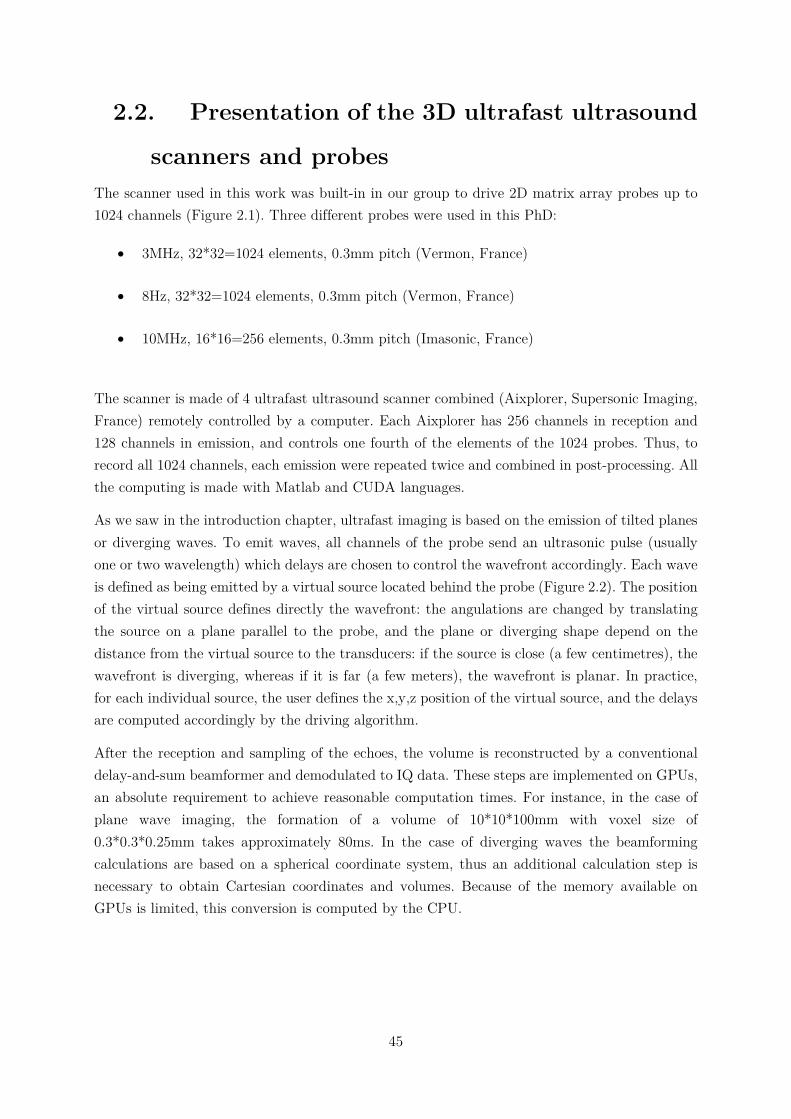
45

2.2. Presentation of the 3D ultrafast ultrasound

scanners and probes The scanner used in this work was built-in in our group to drive 2D matrix array probes up to 1024 channels (Figure 2.1). Three different probes were used in this PhD:

3MHz, 32*32=1024 elements, 0.3mm pitch (Vermon, France)

8Hz, 32*32=1024 elements, 0.3mm pitch (Vermon, France)

10MHz, 16*16=256 elements, 0.3mm pitch (Imasonic, France)

The scanner is made of 4 ultrafast ultrasound scanner combined (Aixplorer, Supersonic Imaging, France) remotely controlled by a computer. Each Aixplorer has 256 channels in reception and 128 channels in emission, and controls one fourth of the elements of the 1024 probes. Thus, to record all 1024 channels, each emission were repeated twice and combined in post-processing. All the computing is made with Matlab and CUDA languages.

As we saw in the introduction chapter, ultrafast imaging is based on the emission of tilted planes or diverging waves. To emit waves, all channels of the probe send an ultrasonic pulse (usually one or two wavelength) which delays are chosen to control the wavefront accordingly. Each wave is defined as being emitted by a virtual source located behind the probe (Figure 2.2). The position of the virtual source defines directly the wavefront: the angulations are changed by translating the source on a plane parallel to the probe, and the plane or diverging shape depend on the distance from the virtual source to the transducers: if the source is close (a few centimetres), the wavefront is diverging, whereas if it is far (a few meters), the wavefront is planar. In practice, for each individual source, the user defines the x,y,z position of the virtual source, and the delays are computed accordingly by the driving algorithm.

After the reception and sampling of the echoes, the volume is reconstructed by a conventional delay-and-sum beamformer and demodulated to IQ data. These steps are implemented on GPUs, an absolute requirement to achieve reasonable computation times. For instance, in the case of plane wave imaging, the formation of a volume of 10*10*100mm with voxel size of 0.3*0.3*0.25mm takes approximately 80ms. In the case of diverging waves the beamforming calculations are based on a spherical coordinate system, thus an additional calculation step is necessary to obtain Cartesian coordinates and volumes. Because of the memory available on GPUs is limited, this conversion is computed by the CPU.

46

Figure 2.1 Ultrasound scanner and probes used in this PhD. Left: 1024 channels ultrafast ultrasound scanner. Top right: 32*32 probe. Both 3MHz and 8MHz have the same design (Vermon France).

Bottom right: 16*16, 10MHz probe (Imasonic, France).

Figure 2.2 Definition of planes or diverging waves emitted by the 2D probes. (a) Transmitted waves are defined as spherical waves emitted by virtual sources located behind the probes’ transducers

arrays. (b) For each individual sources, transmission delays and subapertures are defined. (c) When virtual sources are relatively close to the probe (a few centimetres), small subapertures are chosen and diverging waves are emitted. (d) When sources are located far (several meters), full aperture is

used and plane waves are sent to the medium. Illustration from (Provost et al., 2014)



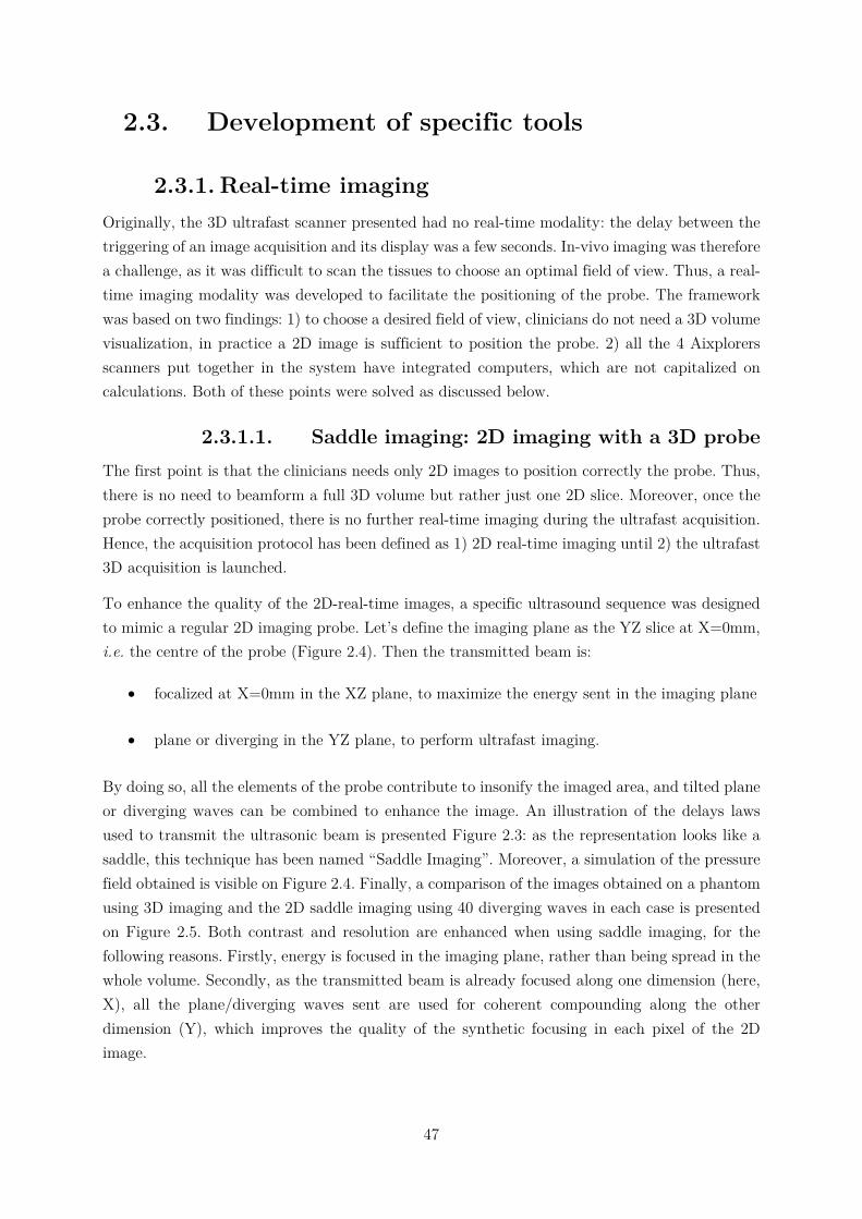
47

2.3. Development of specific tools

2.3.1. Real-time imaging Originally, the 3D ultrafast scanner presented had no real-time modality: the delay between the triggering of an image acquisition and its display was a few seconds. In-vivo imaging was therefore a challenge, as it was difficult to scan the tissues to choose an optimal field of view. Thus, a real-time imaging modality was developed to facilitate the positioning of the probe. The framework was based on two findings: 1) to choose a desired field of view, clinicians do not need a 3D volume visualization, in practice a 2D image is sufficient to position the probe. 2) all the 4 Aixplorers scanners put together in the system have integrated computers, which are not capitalized on calculations. Both of these points were solved as discussed below.

2.3.1.1. Saddle imaging: 2D imaging with a 3D probe The first point is that the clinicians needs only 2D images to position correctly the probe. Thus, there is no need to beamform a full 3D volume but rather just one 2D slice. Moreover, once the probe correctly positioned, there is no further real-time imaging during the ultrafast acquisition. Hence, the acquisition protocol has been defined as 1) 2D real-time imaging until 2) the ultrafast 3D acquisition is launched.

To enhance the quality of the 2D-real-time images, a specific ultrasound sequence was designed to mimic a regular 2D imaging probe. Let’s define the imaging plane as the YZ slice at X=0mm, i.e. the centre of the probe (Figure 2.4). Then the transmitted beam is:

focalized at X=0mm in the XZ plane, to maximize the energy sent in the imaging plane

plane or diverging in the YZ plane, to perform ultrafast imaging.

By doing so, all the elements of the probe contribute to insonify the imaged area, and tilted plane or diverging waves can be combined to enhance the image. An illustration of the delays laws used to transmit the ultrasonic beam is presented Figure 2.3: as the representation looks like a saddle, this technique has been named “Saddle Imaging”. Moreover, a simulation of the pressure field obtained is visible on Figure 2.4. Finally, a comparison of the images obtained on a phantom using 3D imaging and the 2D saddle imaging using 40 diverging waves in each case is presented on Figure 2.5. Both contrast and resolution are enhanced when using saddle imaging, for the following reasons. Firstly, energy is focused in the imaging plane, rather than being spread in the whole volume. Secondly, as the transmitted beam is already focused along one dimension (here, X), all the plane/diverging waves sent are used for coherent compounding along the other dimension (Y), which improves the quality of the synthetic focusing in each pixel of the 2D image.

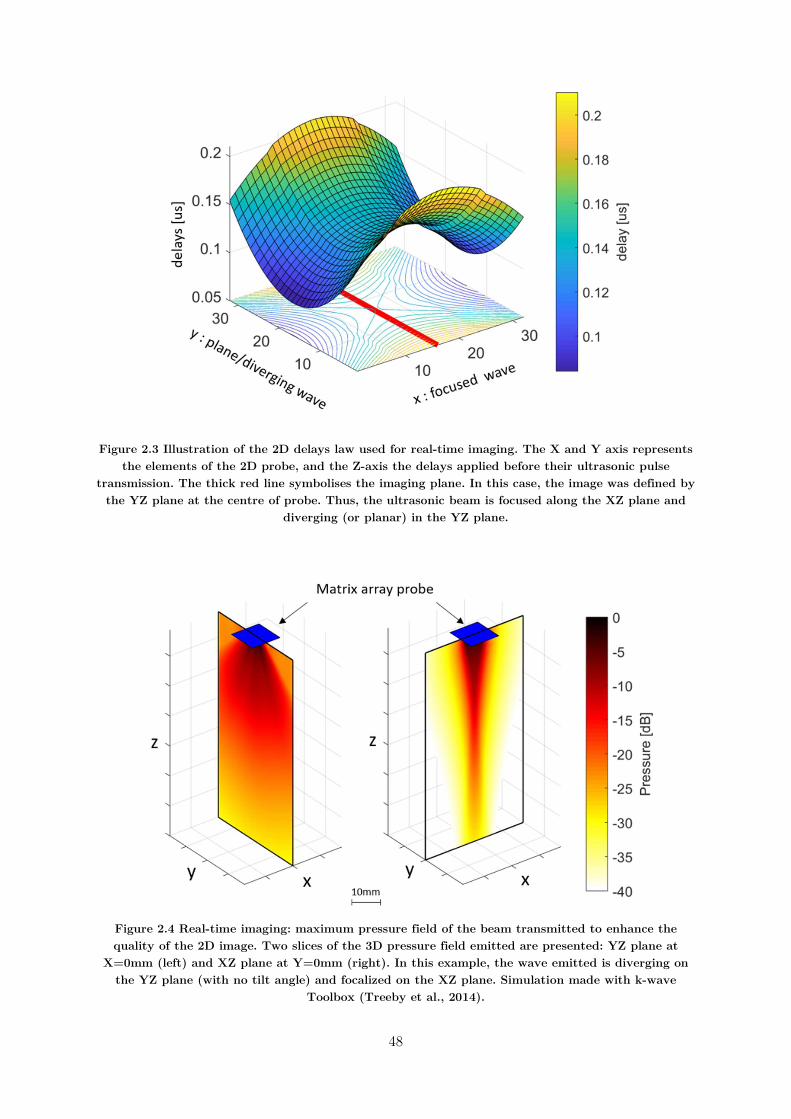
48

Figure 2.3 Illustration of the 2D delays law used for real-time imaging. The X and Y axis represents the elements of the 2D probe, and the Z-axis the delays applied before their ultrasonic pulse

transmission. The thick red line symbolises the imaging plane. In this case, the image was defined by the YZ plane at the centre of probe. Thus, the ultrasonic beam is focused along the XZ plane and

diverging (or planar) in the YZ plane.

Figure 2.4 Real-time imaging: maximum pressure field of the beam transmitted to enhance the quality of the 2D image. Two slices of the 3D pressure field emitted are presented: YZ plane at

X=0mm (left) and XZ plane at Y=0mm (right). In this example, the wave emitted is diverging on the YZ plane (with no tilt angle) and focalized on the XZ plane. Simulation made with k-wave

Toolbox (Treeby et al., 2014).

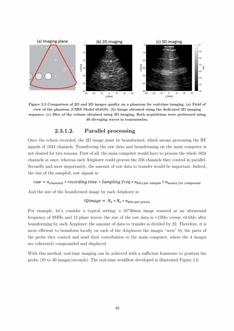
49

Figure 2.5 Comparison of 2D and 3D images quality on a phantom for real-time imaging. (a) Field of view of the phantom (CIRS Model 054GS). (b) Image obtained using the dedicated 2D imaging

sequence. (c) Slice of the volume obtained using 3D imaging. Both acquisitions were performed using 40 diverging waves in transmission.

2.3.1.2. Parallel processing Once the echoes recorded, the 2D image must be beamformed, which means processing the RF signals of 1024 channels. Transferring the raw data and beamforming on the main computer is not desired for two reasons. First of all, the main computer would have to process the whole 1024 channels at once, whereas each Aixplorer could process the 256 channels they control in parallel. Secondly and most importantly, the amount of raw data to transfer would be important. Indeed, the size of the sampled, raw signals is:

𝑟𝑎𝑤 = 𝑛 ∗ 𝑟𝑒𝑐𝑜𝑟𝑑𝑖𝑛𝑔 𝑡𝑖𝑚𝑒 ∗ 𝑆𝑎𝑚𝑝𝑙𝑖𝑛𝑔 𝑓𝑟𝑒𝑞 ∗ 𝑛 ∗ 𝑛

And the size of the beamformed image by each Aixplorer is:

𝐼𝑄𝑖𝑚𝑎𝑔𝑒 = 𝑁 ∗ 𝑁 ∗ 𝑛

For example, let’s consider a typical setting: a 10*30mm image scanned at an ultrasound frequency of 9MHz and 13 plane waves: the size of the raw data is ≈13Mo versus ≈0.6Mo after beamforming by each Aixplorer: the amount of data to transfer is divided by 22. Therefore, it is more efficient to beamform locally on each of the Aixplorers the images “seen” by the parts of the probe they control and send their contribution to the main computer, where the 4 images are coherently compounded and displayed.

With this method, real-time imaging can be achieved with a sufficient framerate to position the probe (10 to 30 images/seconds). The real-time workflow developed is illustrated Figure 2.6.

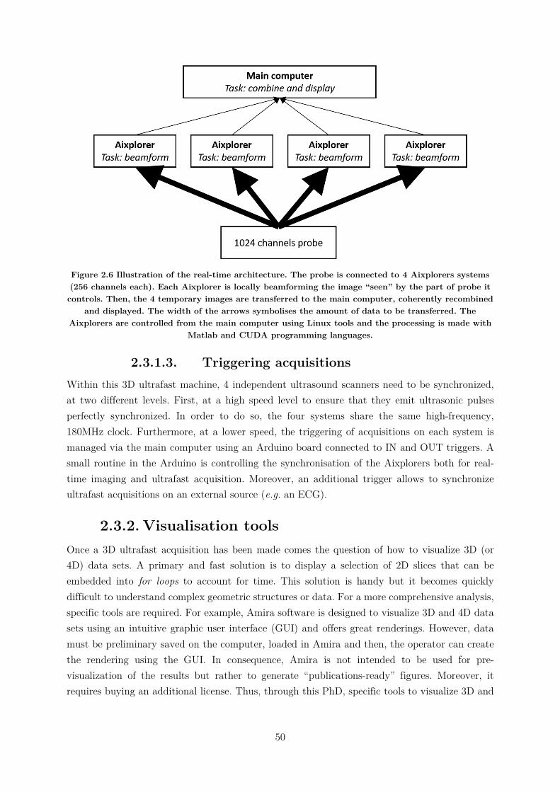
50

Figure 2.6 Illustration of the real-time architecture. The probe is connected to 4 Aixplorers systems (256 channels each). Each Aixplorer is locally beamforming the image “seen” by the part of probe it controls. Then, the 4 temporary images are transferred to the main computer, coherently recombined

and displayed. The width of the arrows symbolises the amount of data to be transferred. The Aixplorers are controlled from the main computer using Linux tools and the processing is made with

Matlab and CUDA programming languages.

2.3.1.3. Triggering acquisitions Within this 3D ultrafast machine, 4 independent ultrasound scanners need to be synchronized, at two different levels. First, at a high speed level to ensure that they emit ultrasonic pulses perfectly synchronized. In order to do so, the four systems share the same high-frequency, 180MHz clock. Furthermore, at a lower speed, the triggering of acquisitions on each system is managed via the main computer using an Arduino board connected to IN and OUT triggers. A small routine in the Arduino is controlling the synchronisation of the Aixplorers both for real-time imaging and ultrafast acquisition. Moreover, an additional trigger allows to synchronize ultrafast acquisitions on an external source (e.g. an ECG).

2.3.2. Visualisation tools Once a 3D ultrafast acquisition has been made comes the question of how to visualize 3D (or 4D) data sets. A primary and fast solution is to display a selection of 2D slices that can be embedded into for loops to account for time. This solution is handy but it becomes quickly difficult to understand complex geometric structures or data. For a more comprehensive analysis, specific tools are required. For example, Amira software is designed to visualize 3D and 4D data sets using an intuitive graphic user interface (GUI) and offers great renderings. However, data must be preliminary saved on the computer, loaded in Amira and then, the operator can create the rendering using the GUI. In consequence, Amira is not intended to be used for pre-visualization of the results but rather to generate “publications-ready” figures. Moreover, it requires buying an additional license. Thus, through this PhD, specific tools to visualize 3D and

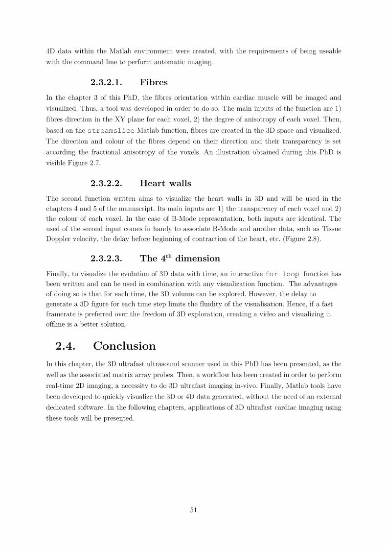
51

4D data within the Matlab environment were created, with the requirements of being useable with the command line to perform automatic imaging.

2.3.2.1. Fibres In the chapter 3 of this PhD, the fibres orientation within cardiac muscle will be imaged and visualized. Thus, a tool was developed in order to do so. The main inputs of the function are 1) fibres direction in the XY plane for each voxel, 2) the degree of anisotropy of each voxel. Then, based on the streamslice Matlab function, fibres are created in the 3D space and visualized. The direction and colour of the fibres depend on their direction and their transparency is set according the fractional anisotropy of the voxels. An illustration obtained during this PhD is visible Figure 2.7.

2.3.2.2. Heart walls The second function written aims to visualize the heart walls in 3D and will be used in the chapters 4 and 5 of the manuscript. Its main inputs are 1) the transparency of each voxel and 2) the colour of each voxel. In the case of B-Mode representation, both inputs are identical. The used of the second input comes in handy to associate B-Mode and another data, such as Tissue Doppler velocity, the delay before beginning of contraction of the heart, etc. (Figure 2.8).

2.3.2.3. The 4th dimension Finally, to visualize the evolution of 3D data with time, an interactive for loop function has been written and can be used in combination with any visualization function. The advantages of doing so is that for each time, the 3D volume can be explored. However, the delay to generate a 3D figure for each time step limits the fluidity of the visualisation. Hence, if a fast framerate is preferred over the freedom of 3D exploration, creating a video and visualizing it offline is a better solution.

2.4. Conclusion In this chapter, the 3D ultrafast ultrasound scanner used in this PhD has been presented, as the well as the associated matrix array probes. Then, a workflow has been created in order to perform real-time 2D imaging, a necessity to do 3D ultrafast imaging in-vivo. Finally, Matlab tools have been developed to quickly visualize the 3D or 4D data generated, without the need of an external dedicated software. In the following chapters, applications of 3D ultrafast cardiac imaging using these tools will be presented.

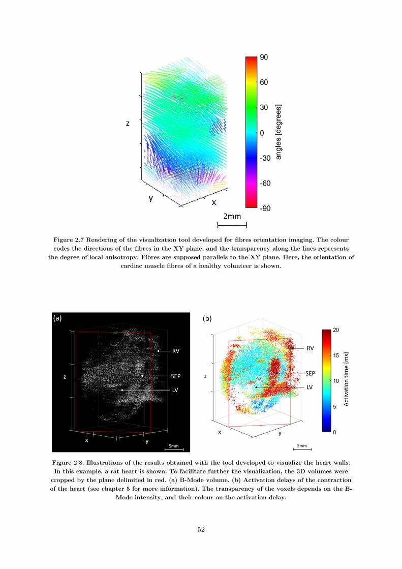
52

Figure 2.7 Rendering of the visualization tool developed for fibres orientation imaging. The colour codes the directions of the fibres in the XY plane, and the transparency along the lines represents

the degree of local anisotropy. Fibres are supposed parallels to the XY plane. Here, the orientation of cardiac muscle fibres of a healthy volunteer is shown.

Figure 2.8. Illustrations of the results obtained with the tool developed to visualize the heart walls. In this example, a rat heart is shown. To facilitate further the visualization, the 3D volumes were

cropped by the plane delimited in red. (a) B-Mode volume. (b) Activation delays of the contraction of the heart (see chapter 5 for more information). The transparency of the voxels depends on the B-

Mode intensity, and their colour on the activation delay.

53


Bercoff, J., Tanter, M., Fink, M., 2004. Supersonic shear imaging: a new technique for soft tissue elasticity mapping. IEEE Transactions on Ultrasonics, Ferroelectrics and Frequency Control 51, 396–409. https://doi.org/10.1109/TUFFC.2004.1295425

Couade, M., Pernot, M., Tanter, M., Messas, E., Bel, A., Ba, M., Hagege, A.-A., Fink, M., 2009. Ultrafast imaging of the heart using circular wave synthetic imaging with phased arrays 515–518. https://doi.org/10.1109/ultsym.2009.5441640

Demené, C., Pernot, M., Biran, V., Alison, M., Fink, M., Baud, O., Tanter, M., 2014. Ultrafast Doppler Reveals the Mapping of Cerebral Vascular Resistivity in Neonates. Journal of Cerebral Blood Flow & Metabolism 34, 1009–1017. https://doi.org/10.1038/jcbfm.2014.49

Fujikura, K., Luo, J., Gamarnik, V., Pernot, M., Fukumoto, R., Tilson, M.D., Konofagou, E.E., 2007. A Novel Noninvasive Technique for Pulse-Wave Imaging and Characterization of Clinically-Significant Vascular Mechanical Properties In Vivo. Ultrasonic Imaging 29, 137–154. https://doi.org/10.1177/016173460702900301

Honjo, Y., Hasegawa, H., Kanai, H., 2010. Two-Dimensional Tracking of Heart Wall for Detailed Analysis of Heart Function at High Temporal and Spatial Resolutions. Japanese Journal of Applied Physics 49, 07HF14. https://doi.org/10.1143/JJAP.49.07HF14

Konofagou, E., Lee, W.-N., Luo, J., Provost, J., Vappou, J., 2011. Physiologic Cardiovascular Strain and Intrinsic Wave Imaging. Annual Review of Biomedical Engineering 13, 477–505. https://doi.org/10.1146/annurev-bioeng-071910-124721

Lang, R.M., Badano, L.P., Tsang, W., Adams, D.H., Agricola, E., Buck, T., Faletra, F.F., Franke, A., Hung, J., de Isla, L.P., Kamp, O., Kasprzak, J.D., Lancellotti, P., Marwick, T.H., McCulloch, M.L., Monaghan, M.J., Nihoyannopoulos, P., Pandian, N.G., Pellikka, P.A., Pepi, M., Roberson, D.A., Shernan, S.K., Shirali, G.S., Sugeng, L., Ten Cate, F.J., Vannan, M.A., Zamorano, J.L., Zoghbi, W.A., 2012. EAE/ASE Recommendations for Image Acquisition and Display Using Three-Dimensional Echocardiography. European Heart Journal - Cardiovascular Imaging 13, 1–46. https://doi.org/10.1093/ehjci/jer316

Macé, E., Montaldo, G., Cohen, I., Baulac, M., Fink, M., Tanter, M., 2011. Functional ultrasound imaging of the brain. Nature Methods 8, 662–664. https://doi.org/10.1038/nmeth.1641

Mallart, R., Fink, M., 1992. Improved imaging rate through simultaneous transmission of several ultrasound beams, in: Lizzi, F.L. (Ed.), . Presented at the San Diego ’92, San Diego, CA, pp. 120–130. https://doi.org/10.1117/12.130591

Osmanski, B.F., Martin, C., Montaldo, G., Lanièce, P., Pain, F., Tanter, M., Gurden, H., 2014. Functional ultrasound imaging reveals different odor-evoked patterns of vascular activity

54

in the main olfactory bulb and the anterior piriform cortex. NeuroImage 95, 176–184. https://doi.org/10.1016/j.neuroimage.2014.03.054

Papadacci, C., Pernot, M., Couade, M., Fink, M., Tanter, M., 2014. High-contrast ultrafast imaging of the heart. IEEE Transactions on Ultrasonics, Ferroelectrics, and Frequency Control 61, 288–301. https://doi.org/10.1109/TUFFC.2014.6722614

Pernot, M., Fujikura, K., Fung-Kee-Fung, S.D., Konofagou, E.E., 2007. ECG-gated, Mechanical and Electromechanical Wave Imaging of Cardiovascular Tissues In Vivo. Ultrasound in Medicine & Biology 33, 1075–1085. https://doi.org/10.1016/j.ultrasmedbio.2007.02.003

Provost, J., Gambhir, A., Vest, J., Garan, H., Konofagou, E.E., 2013. A clinical feasibility study of atrial and ventricular electromechanical wave imaging. Heart Rhythm 10, 856–862. https://doi.org/10.1016/j.hrthm.2013.02.028

Provost, J., Lee, W.-N., Fujikura, K., Konofagou, E.E., 2011a. Imaging the electromechanical activity of the heart in vivo. Proceedings of the National Academy of Sciences 108, 8565–8570.

Provost, J., Nguyen, V.T.-H., Legrand, D., Okrasinski, S., Costet, A., Gambhir, A., Garan, H., Konofagou, E.E., 2011b. Electromechanical wave imaging for arrhythmias. Physics in Medicine and Biology 56, L1–L11. https://doi.org/10.1088/0031-9155/56/22/F01


Provost, J., Wei-Ning Lee, Fujikura, K., Konofagou, E.E., 2010. Electromechanical Wave Imaging of Normal and Ischemic Hearts In Vivo. IEEE Transactions on Medical Imaging 29, 625–635. https://doi.org/10.1109/TMI.2009.2030186


Sandrin, L., Tanter, M., Catheline, S., Fink, M., 2002. Shear modulus imaging with 2-D transient elastography. IEEE Transactions on Ultrasonics, Ferroelectrics and Frequency Control 49, 426–435. https://doi.org/10.1109/58.996560

Shougang Wang, Wei-ning Lee, Provost, J., Jianwen Luo, Konofagou, E.E., 2008. A composite high-frame-rate system for clinical cardiovascular imaging. IEEE Transactions on Ultrasonics, Ferroelectrics and Frequency Control 55, 2221–2233. https://doi.org/10.1109/TUFFC.921

Tanter, M., Bercoff, J., Athanasiou, A., Deffieux, T., Gennisson, J.-L., Montaldo, G., Muller, M., Tardivon, A., Fink, M., 2008. Quantitative Assessment of Breast Lesion Viscoelasticity:

55

Initial Clinical Results Using Supersonic Shear Imaging. Ultrasound in Medicine & Biology 34, 1373–1386. https://doi.org/10.1016/j.ultrasmedbio.2008.02.002

Tanter, M., Bercoff, J., Sandrin, L., Fink, M., 2002. Ultrafast compound imaging for 2-D motion vector estimation: application to transient elastography. IEEE Transactions on Ultrasonics, Ferroelectrics and Frequency Control 49, 1363–1374. https://doi.org/10.1109/TUFFC.2002.1041078

Tong, L., Gao, H., D’hooge, J., 2013. Multi-transmit beam forming for fast cardiac imaging-a simulation study. IEEE Transactions on Ultrasonics, Ferroelectrics, and Frequency Control 60, 1719–1731. https://doi.org/10.1109/TUFFC.2013.2753

Tong, L., Ramalli, A., Jasaityte, R., Tortoli, P., D’hooge, J., 2014. Multi-Transmit Beam Forming for Fast Cardiac Imaging—Experimental Validation and In Vivo Application. IEEE Transactions on Medical Imaging 33, 1205–1219. https://doi.org/10.1109/TMI.2014.2302312

Treeby, B.E., Jaros, J., Rohrbach, D., Cox, B.T., 2014. Modelling elastic wave propagation using the k-Wave MATLAB Toolbox. IEEE, pp. 146–149. https://doi.org/10.1109/ULTSYM.2014.0037

Yagel, S., Cohen, S.M., Shapiro, I., Valsky, D.V., 2007. 3D and 4D ultrasound in fetal cardiac scanning: a new look at the fetal heart. Ultrasound in Obstetrics & Gynecology 29, 81–95. https://doi.org/10.1002/uog.3912

57

: 3D Backscatter Tensor

Imaging 3. : 3D Backscatter Tensor Imaging ....................................................................................... 57

3.1. Introduction…..………………………………………………………………………………………………………………………….. 58

3.1.1. Motivations .......................................................................................................... 58

3.1.2. State of the art ..................................................................................................... 58

3.1.2.1. The fibers architecture of the heart .............................................................. 58

3.1.2.2. Imaging the fibers architecture ..................................................................... 60

3.1.2.3. Spatial coherence of ultrasonic backscattered echoes .................................... 63

3.1.3. Objectives ............................................................................................................. 66

3.2. 3D Mapping of cardiac fibres orientation ……………………………………………………………………………..66


3.2.1.1. Spatial coherence on a matrix array transducer ........................................... 66

3.2.1.2. Coherent compounding of plane waves for 3D-BTI ...................................... 67

3.2.1.3. Analysis of the 2D coherence function using the Radon transform .............. 68

3.2.1.4. Experimental Setup ...................................................................................... 69

3.2.2. Results ................................................................................................................. 69

3.2.3. Discussion ............................................................................................................. 72

3.3. Correction of aberrations due to movement ………………………………………………………………………. 72


3.3.1.1. Motion estimation and correction ................................................................. 73

3.3.1.2. Phantom study: experimental setup ............................................................. 75

3.3.1.3. In-vivo application: experimental setup ........................................................ 76

3.3.2. Results ................................................................................................................. 76

3.3.2.1. Phantom study ............................................................................................. 76

3.3.2.2. In-vivo study ................................................................................................. 79

3.3.3. Discussion ............................................................................................................. 79

3.4. Conclusion ………………………………………………………………………………………………………………………………… 82

3.5. Chapter bibliography ……………………………………………………………………………………………………………… 83

58

3D Backscatter Tensor Imaging

3.1. Introduction In this chapter, we will develop 3D Backscatter Tensor Imaging (3D BTI), a technique to image the orientation of myocardial fibres using a 4D ultrafast ultrasound scanner. This work is the direct continuation of Clement Papadacci’s PhD thesis (Papadacci, 2014), in which he showed the feasibility of using 3D BTI to image the orientation of cardiac fibres in open-chest pigs. In this chapter, we will firstly show the application of 3D-BTI transthoracically on healthy volunteers, which we published as the two co-first authors (Papadacci et al., 2017). Then, a methodology to reduce movement artefacts will be introduced.

3.1.1. Motivations The myocardial fibres architecture plays a major role in the cardiac function. Fibres orientations vary continuously and smoothly through myocardial walls (Streeter and Bassett, 1966) and this complex organization is closely linked to the mechanical and electrical myocardial function (Arts et al., 2001; Costa et al., 1999; Waldman et al., 1988). For instance, the helicoidal fibres distribution in the left ventricular walls contributes to the torsional motion of the heart during the ejection phase, which is believed to improve the heart’s pumping efficiency (Hansen et al., 1991; Taber et al., 1996). The fibres of the heart are also related to its electromechanical properties (Hooks et al., 2007; Kadish et al., 1988; Roberts et al., 1979; Taccardi et al., 1994): indeed, the electrical activation propagates preferentially in the direction of myocardial fibres and results in their synchronous contraction. Myocardial fibre disarray is thought to appear in the early stage of many pathologies such as in cardiomyopathies or fibrosis (Tseng et al., 2006). The mapping of the fibre architecture, on the one hand, could increase our knowledge of the cardiac function (Savadjiev et al., 2012), and on the other hand, could potentially enable early diagnosis of cardiomyopathies. Yet, no method to map the fibre architecture is currently used on a regular basis for clinical purposes.

3.1.2. State of the art

3.1.2.1. The fibres architecture of the heart The heart muscle, the myocardium, is a complex three dimensional structure forming a thick middle layer between the outer layer of the heart wall (the epicardium) and the inner layer (the endocardium). It is composed of individual heart muscle cells (cardiomyocytes, often simply called myocytes) and collagen cells. The myocytes are roughly rectangular cells measuring 100–150µm by 30–40µm, and are linked together by intercalated discs to form continuous fibres. The fibres are regrouped together in layers 3 to 4 myocytes thick called sheets (Bers, 2001), themselves stacked between collagen fibres (see figure 3.1).

59

Figure 3.1 Architecture of the cardiac muscle. A transmural block cut from the ventricular wall shows the orientation of fibres through the wall. (b) The muscle fibres are shown forming a sheet three to four cells thick. Collagen connects adjacent cells within a sheet, as well as adjacent sheet.

Figure modified from (Legrice et al., 2001).

The orientation of the fibers varies through the wall, forming an helix with an angle between the epicardium and endocardium of the order of 120° (Streeter and Bassett, 1966) (see figure 3.2). To eject blood, the myocytes contract and shorten, leading to a twisting of the left ventricle. The orientation of the myocytes is thus fundamental to ensure the efficiency of the blood ejection. Moreover, the fibers of the heart are also related to its activation sequence (Hooks et al., 2007; Kadish et al., 1988; Roberts et al., 1979; Taccardi et al., 1994) as the electrical activation propagates faster along the direction of myocytes rather than perpendicularly.

Figure 3.2 Schematic representation of the fibers orientation through the left ventricle wall. The fibres angles varies from –α at the epicardium (epi) to +α at the endocardium (endo). The order of magnitude of α is ≈60°. By convention, the circumferential fibres of the midwall have an angle of

α=0°. Adapted from (Nguyen et al., 2018).





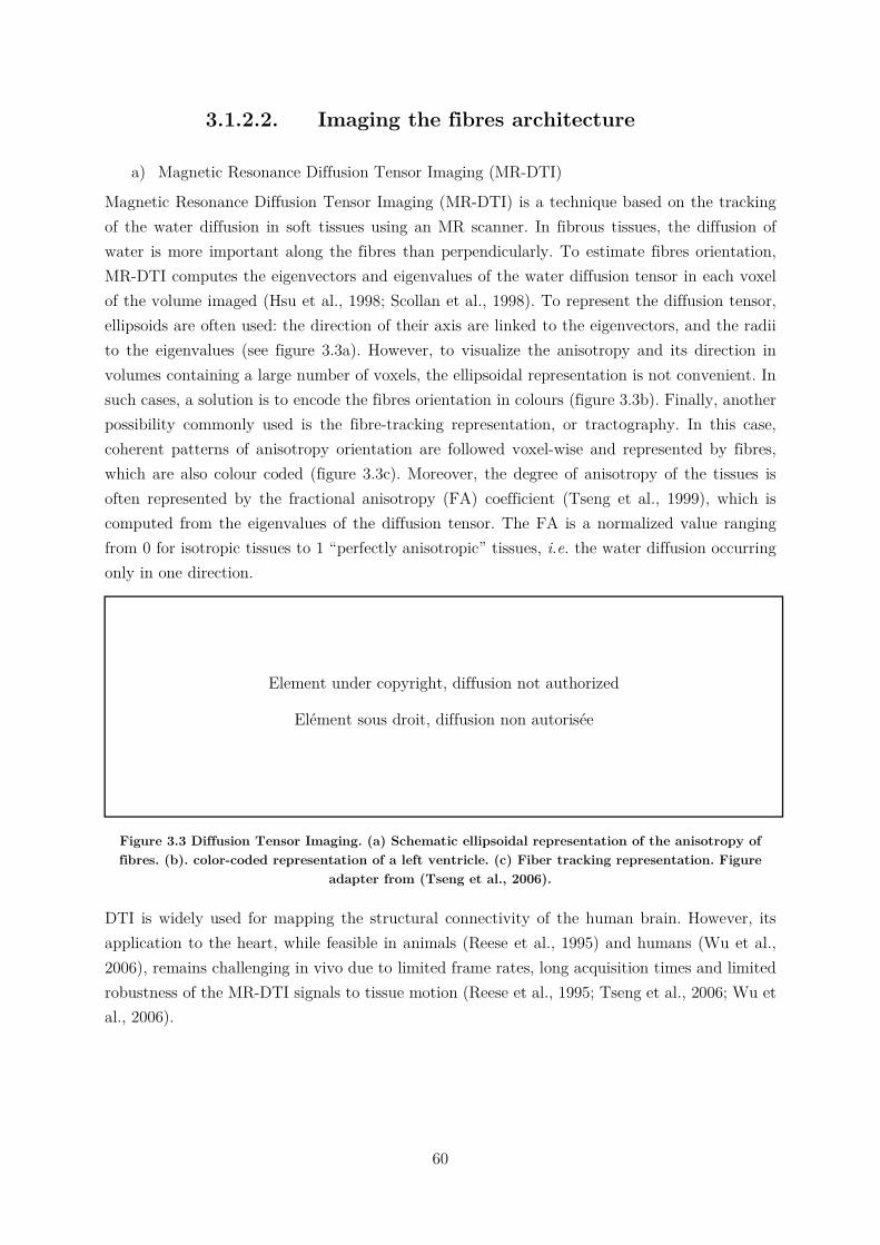
60

3.1.2.2. Imaging the fibres architecture

a) Magnetic Resonance Diffusion Tensor Imaging (MR-DTI)

Magnetic Resonance Diffusion Tensor Imaging (MR-DTI) is a technique based on the tracking of the water diffusion in soft tissues using an MR scanner. In fibrous tissues, the diffusion of water is more important along the fibres than perpendicularly. To estimate fibres orientation, MR-DTI computes the eigenvectors and eigenvalues of the water diffusion tensor in each voxel of the volume imaged (Hsu et al., 1998; Scollan et al., 1998). To represent the diffusion tensor, ellipsoids are often used: the direction of their axis are linked to the eigenvectors, and the radii to the eigenvalues (see figure 3.3a). However, to visualize the anisotropy and its direction in volumes containing a large number of voxels, the ellipsoidal representation is not convenient. In such cases, a solution is to encode the fibres orientation in colours (figure 3.3b). Finally, another possibility commonly used is the fibre-tracking representation, or tractography. In this case, coherent patterns of anisotropy orientation are followed voxel-wise and represented by fibres, which are also colour coded (figure 3.3c). Moreover, the degree of anisotropy of the tissues is often represented by the fractional anisotropy (FA) coefficient (Tseng et al., 1999), which is computed from the eigenvalues of the diffusion tensor. The FA is a normalized value ranging from 0 for isotropic tissues to 1 “perfectly anisotropic” tissues, i.e. the water diffusion occurring only in one direction.

Figure 3.3 Diffusion Tensor Imaging. (a) Schematic ellipsoidal representation of the anisotropy of fibres. (b). color-coded representation of a left ventricle. (c) Fiber tracking representation. Figure

adapter from (Tseng et al., 2006).

DTI is widely used for mapping the structural connectivity of the human brain. However, its application to the heart, while feasible in animals (Reese et al., 1995) and humans (Wu et al., 2006), remains challenging in vivo due to limited frame rates, long acquisition times and limited robustness of the MR-DTI signals to tissue motion (Reese et al., 1995; Tseng et al., 2006; Wu et al., 2006).



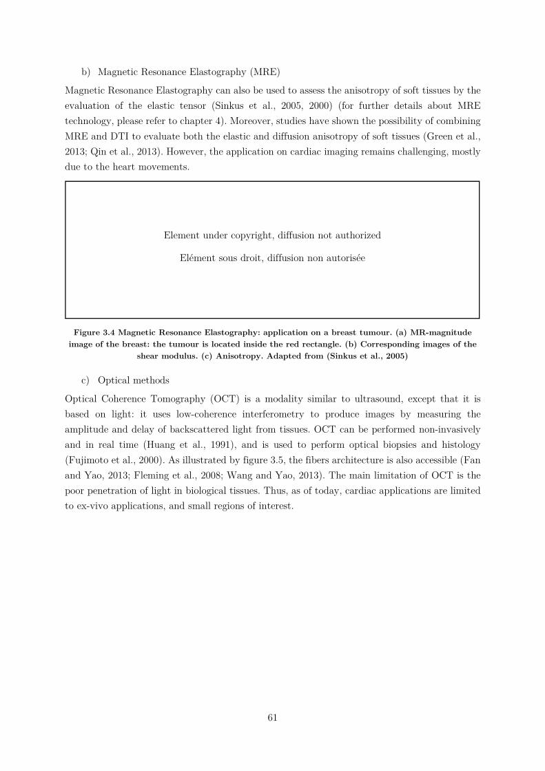
61

b) Magnetic Resonance Elastography (MRE)

Magnetic Resonance Elastography can also be used to assess the anisotropy of soft tissues by the evaluation of the elastic tensor (Sinkus et al., 2005, 2000) (for further details about MRE technology, please refer to chapter 4). Moreover, studies have shown the possibility of combining MRE and DTI to evaluate both the elastic and diffusion anisotropy of soft tissues (Green et al., 2013; Qin et al., 2013). However, the application on cardiac imaging remains challenging, mostly due to the heart movements.

Figure 3.4 Magnetic Resonance Elastography: application on a breast tumour. (a) MR-magnitude image of the breast: the tumour is located inside the red rectangle. (b) Corresponding images of the

shear modulus. (c) Anisotropy. Adapted from (Sinkus et al., 2005)

c) Optical methods

Optical Coherence Tomography (OCT) is a modality similar to ultrasound, except that it is based on light: it uses low-coherence interferometry to produce images by measuring the amplitude and delay of backscattered light from tissues. OCT can be performed non-invasively and in real time (Huang et al., 1991), and is used to perform optical biopsies and histology (Fujimoto et al., 2000). As illustrated by figure 3.5, the fibers architecture is also accessible (Fan and Yao, 2013; Fleming et al., 2008; Wang and Yao, 2013). The main limitation of OCT is the poor penetration of light in biological tissues. Thus, as of today, cardiac applications are limited to ex-vivo applications, and small regions of interest.



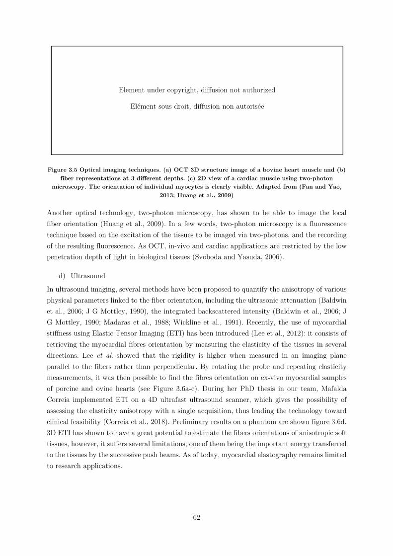
62

Figure 3.5 Optical imaging techniques. (a) OCT 3D structure image of a bovine heart muscle and (b) fiber representations at 3 different depths. (c) 2D view of a cardiac muscle using two-photon

microscopy. The orientation of individual myocytes is clearly visible. Adapted from (Fan and Yao, 2013; Huang et al., 2009)

Another optical technology, two-photon microscopy, has shown to be able to image the local fiber orientation (Huang et al., 2009). In a few words, two-photon microscopy is a fluorescence technique based on the excitation of the tissues to be imaged via two-photons, and the recording of the resulting fluorescence. As OCT, in-vivo and cardiac applications are restricted by the low penetration depth of light in biological tissues (Svoboda and Yasuda, 2006).

d) Ultrasound

In ultrasound imaging, several methods have been proposed to quantify the anisotropy of various physical parameters linked to the fiber orientation, including the ultrasonic attenuation (Baldwin et al., 2006; J G Mottley, 1990), the integrated backscattered intensity (Baldwin et al., 2006; J G Mottley, 1990; Madaras et al., 1988; Wickline et al., 1991). Recently, the use of myocardial stiffness using Elastic Tensor Imaging (ETI) has been introduced (Lee et al., 2012): it consists of retrieving the myocardial fibres orientation by measuring the elasticity of the tissues in several directions. Lee et al. showed that the rigidity is higher when measured in an imaging plane parallel to the fibers rather than perpendicular. By rotating the probe and repeating elasticity measurements, it was then possible to find the fibres orientation on ex-vivo myocardial samples of porcine and ovine hearts (see Figure 3.6a-c). During her PhD thesis in our team, Mafalda Correia implemented ETI on a 4D ultrafast ultrasound scanner, which gives the possibility of assessing the elasticity anisotropy with a single acquisition, thus leading the technology toward clinical feasibility (Correia et al., 2018). Preliminary results on a phantom are shown figure 3.6d. 3D ETI has shown to have a great potential to estimate the fibers orientations of anisotropic soft tissues, however, it suffers several limitations, one of them being the important energy transferred to the tissues by the successive push beams. As of today, myocardial elastography remains limited to research applications.



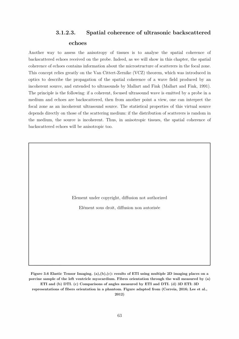
63

3.1.2.3. Spatial coherence of ultrasonic backscattered

echoes Another way to assess the anisotropy of tissues is to analyse the spatial coherence of backscattered echoes received on the probe. Indeed, as we will show in this chapter, the spatial coherence of echoes contains information about the microstructure of scatterers in the focal zone. This concept relies greatly on the Van Cittert-Zernike (VCZ) theorem, which was introduced in optics to describe the propagation of the spatial coherence of a wave field produced by an incoherent source, and extended to ultrasounds by Mallart and Fink (Mallart and Fink, 1991). The principle is the following: if a coherent, focused ultrasound wave is emitted by a probe in a medium and echoes are backscattered, then from another point a view, one can interpret the focal zone as an incoherent ultrasound source. The statistical properties of this virtual source depends directly on those of the scattering medium: if the distribution of scatterers is random in the medium, the source is incoherent. Thus, in anisotropic tissues, the spatial coherence of backscattered echoes will be anisotropic too.

Figure 3.6 Elastic Tensor Imaging. (a),(b),(c): results of ETI using multiple 2D imaging places on a porcine sample of the left ventricle myocardium. Fibres orientation through the wall measured by (a)

ETI and (b) DTI. (c) Comparisons of angles measured by ETI and DTI. (d) 3D ETI: 3D representations of fibers orientation in a phantom. Figure adapted from (Correia, 2016; Lee et al.,

2012)



64

In medical ultrasound, the spatial coherence of backscattered echoes has found diverse applications, such as aberration correction (Hollman et al., 1999; Mallart and Fink, 1994; Walker and Trahey, 1997), sound velocity estimation (Imbault et al., 2017; Pai-Chi Li and Meng-Lin Li, 2003) or image formation (Dahl et al., 2012; Lediju et al., 2011). In particular, Derode and Fink suggested the use of spatial coherence to characterize the distribution of scatterers in fibrous composite materials (Derode and Fink, 1993). In their study, they showed that the spatial coherence of echoes received by the elements of the ultrasonic probe decreased faster with the distance between elements when the probe is perpendicular to the fibers rather than parallel (see figure 3.7).

Later in our group, Clement Papadacci continued this work and applied it to the estimation of fibres orientation in biological tissues, and in particular to ex-vivo porcine and bovine myocardium (Papadacci et al., 2014a). In an analogy to DTI and ETI, this technique was named BTI, standing for Backscatter Tensor Imaging. The main limitation of this work was the use of a linear transducer, implying the need to rotate the array to perform an acquisition, making difficult its use in a clinical setting. In order to overcome this limit, BTI was implemented on a 2D matrix transducer to be able to retrieve the spatial coherence in all directions parallel to the transducer’s plane within a single acquisition (3D-BTI). At the end of his PhD in 2014, Papadacci had proven the accuracy of BTI against histological measurements on ex-vivo porcine hearts (figure 3.8) and shown the feasibility of using 3D-BTI to estimate the fibres orientation in the mid-anterior region of the LV of open-chest ovine and during the cardiac cycle (figure 3.9).

Figure 3.7 Derode and Fink study on fibrous composite materials. (a) Experimental setup. The linear ultrasonic array is rotated to repeat pule-echo measurements for different probe/fibres angles. (b) Evolutions of inter-elements spatial coherence depending on the distance between the elements and

on the orientation of the probe with respect to the fibres of the material. The spatial coherence decreased faster when the probe is perpendicular to the fibers. Figure adapted from (Derode and

Fink, 1993).



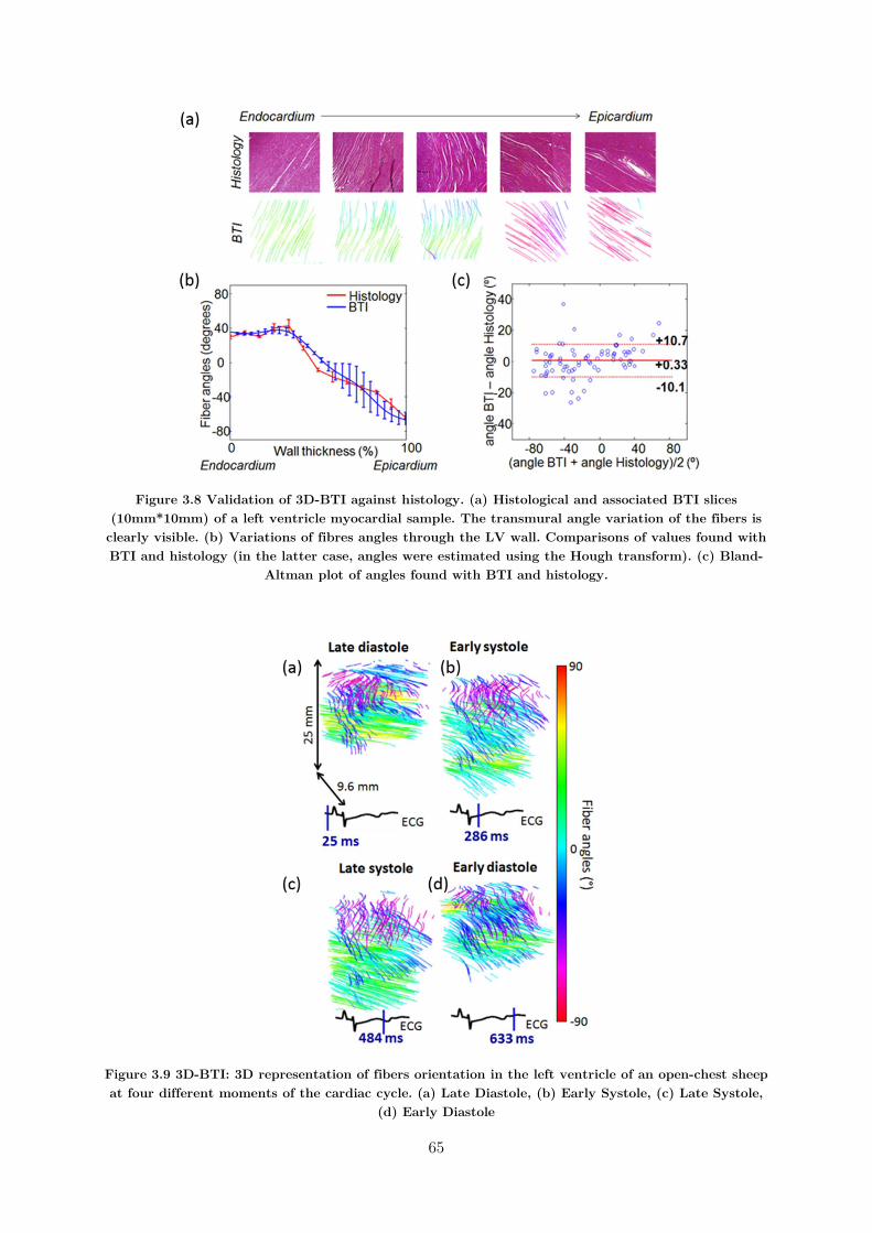
65

Figure 3.8 Validation of 3D-BTI against histology. (a) Histological and associated BTI slices (10mm*10mm) of a left ventricle myocardial sample. The transmural angle variation of the fibers is clearly visible. (b) Variations of fibres angles through the LV wall. Comparisons of values found with BTI and histology (in the latter case, angles were estimated using the Hough transform). (c) Bland-

Altman plot of angles found with BTI and histology.

Figure 3.9 3D-BTI: 3D representation of fibers orientation in the left ventricle of an open-chest sheep at four different moments of the cardiac cycle. (a) Late Diastole, (b) Early Systole, (c) Late Systole,

(d) Early Diastole

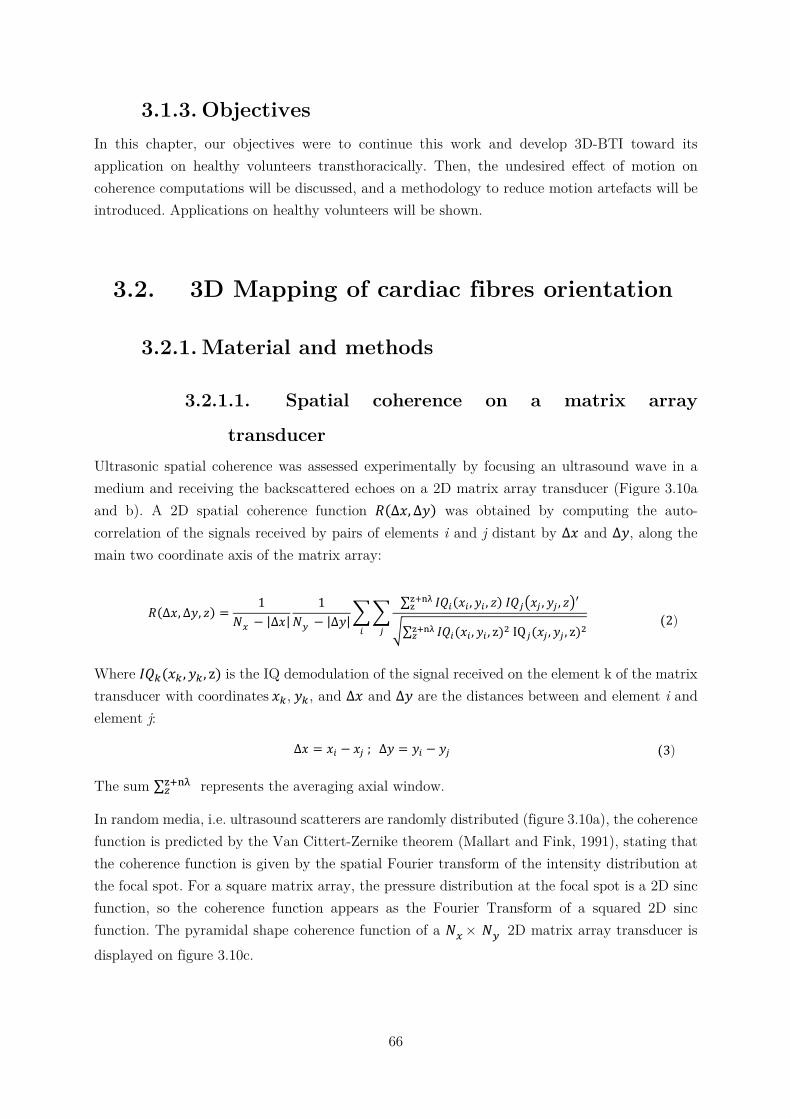
66

3.1.3. Objectives In this chapter, our objectives were to continue this work and develop 3D-BTI toward its application on healthy volunteers transthoracically. Then, the undesired effect of motion on coherence computations will be discussed, and a methodology to reduce motion artefacts will be introduced. Applications on healthy volunteers will be shown.

3.2. 3D Mapping of cardiac fibres orientation

3.2.1. Material and methods

3.2.1.1. Spatial coherence on a matrix array

transducer Ultrasonic spatial coherence was assessed experimentally by focusing an ultrasound wave in a medium and receiving the backscattered echoes on a 2D matrix array transducer (Figure 3.10a and b). A 2D spatial coherence function 𝑅(∆𝑥, ∆𝑦) was obtained by computing the auto-correlation of the signals received by pairs of elements i and j distant by ∆𝑥 and ∆𝑦, along the main two coordinate axis of the matrix array:

𝑅(∆𝑥, ∆𝑦, 𝑧) =1

𝑁 − |∆𝑥|

1

𝑁 − |∆𝑦|

∑ 𝐼𝑄 (𝑥 , 𝑦 , 𝑧) 𝐼𝑄 𝑥 , 𝑦 , 𝑧 ′

∑ 𝐼𝑄 (𝑥 , 𝑦 , z) IQ (𝑥 , 𝑦 , z)

(2)

Where 𝐼𝑄 (𝑥 , 𝑦 , z) is the IQ demodulation of the signal received on the element k of the matrix transducer with coordinates 𝑥 , 𝑦 , and ∆𝑥 and ∆𝑦 are the distances between and element i and element j:

∆𝑥 = 𝑥 − 𝑥 ; ∆𝑦 = 𝑦 − 𝑦 (3)

The sum ∑ represents the averaging axial window.

In random media, i.e. ultrasound scatterers are randomly distributed (figure 3.10a), the coherence function is predicted by the Van Cittert-Zernike theorem (Mallart and Fink, 1991), stating that the coherence function is given by the spatial Fourier transform of the intensity distribution at the focal spot. For a square matrix array, the pressure distribution at the focal spot is a 2D sinc function, so the coherence function appears as the Fourier Transform of a squared 2D sinc function. The pyramidal shape coherence function of a 𝑁 × 𝑁 2D matrix array transducer is displayed on figure 3.10c.

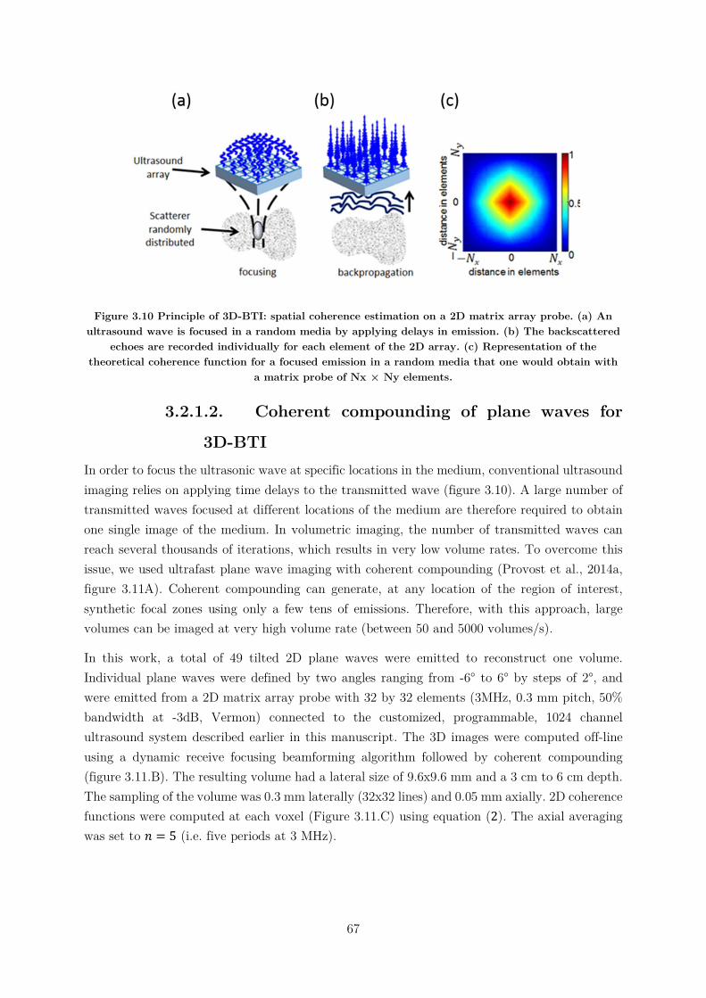
67

Figure 3.10 Principle of 3D-BTI: spatial coherence estimation on a 2D matrix array probe. (a) An ultrasound wave is focused in a random media by applying delays in emission. (b) The backscattered

echoes are recorded individually for each element of the 2D array. (c) Representation of the theoretical coherence function for a focused emission in a random media that one would obtain with

a matrix probe of Nx × Ny elements.

3.2.1.2. Coherent compounding of plane waves for

3D-BTI In order to focus the ultrasonic wave at specific locations in the medium, conventional ultrasound imaging relies on applying time delays to the transmitted wave (figure 3.10). A large number of transmitted waves focused at different locations of the medium are therefore required to obtain one single image of the medium. In volumetric imaging, the number of transmitted waves can reach several thousands of iterations, which results in very low volume rates. To overcome this issue, we used ultrafast plane wave imaging with coherent compounding (Provost et al., 2014a, figure 3.11A). Coherent compounding can generate, at any location of the region of interest, synthetic focal zones using only a few tens of emissions. Therefore, with this approach, large volumes can be imaged at very high volume rate (between 50 and 5000 volumes/s).

In this work, a total of 49 tilted 2D plane waves were emitted to reconstruct one volume. Individual plane waves were defined by two angles ranging from -6° to 6° by steps of 2°, and were emitted from a 2D matrix array probe with 32 by 32 elements (3MHz, 0.3 mm pitch, 50% bandwidth at -3dB, Vermon) connected to the customized, programmable, 1024 channel ultrasound system described earlier in this manuscript. The 3D images were computed off-line using a dynamic receive focusing beamforming algorithm followed by coherent compounding (figure 3.11.B). The resulting volume had a lateral size of 9.6x9.6 mm and a 3 cm to 6 cm depth. The sampling of the volume was 0.3 mm laterally (32x32 lines) and 0.05 mm axially. 2D coherence functions were computed at each voxel (Figure 3.11.C) using equation (2). The axial averaging was set to 𝑛 = 5 (i.e. five periods at 3 MHz).

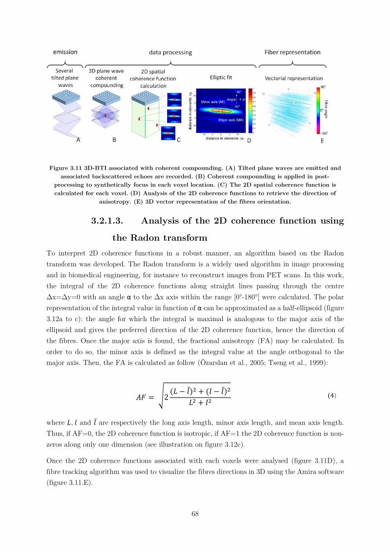
68

Figure 3.11 3D-BTI associated with coherent compounding. (A) Tilted plane waves are emitted and associated backscattered echoes are recorded. (B) Coherent compounding is applied in post-

processing to synthetically focus in each voxel location. (C) The 2D spatial coherence function is calculated for each voxel. (D) Analysis of the 2D coherence functions to retrieve the direction of

anisotropy. (E) 3D vector representation of the fibres orientation.

3.2.1.3. Analysis of the 2D coherence function using

the Radon transform To interpret 2D coherence functions in a robust manner, an algorithm based on the Radon transform was developed. The Radon transform is a widely used algorithm in image processing and in biomedical engineering, for instance to reconstruct images from PET scans. In this work, the integral of the 2D coherence functions along straight lines passing through the centre Δx=Δy=0 with an angle α to the Δx axis within the range [0°-180°[ were calculated. The polar representation of the integral value in function of α can be approximated as a half-ellipsoid (figure 3.12a to c): the angle for which the integral is maximal is analogous to the major axis of the ellipsoid and gives the preferred direction of the 2D coherence function, hence the direction of the fibres. Once the major axis is found, the fractional anisotropy (FA) may be calculated. In order to do so, the minor axis is defined as the integral value at the angle orthogonal to the major axis. Then, the FA is calculated as follow (Özarslan et al., 2005; Tseng et al., 1999):

𝐴𝐹 = 2(𝐿 − 𝑙)̅ + (𝑙 − 𝑙)̅

𝐿 + 𝑙 (4)

where 𝐿, 𝑙 and 𝑙 ̅are respectively the long axis length, minor axis length, and mean axis length. Thus, if AF=0, the 2D coherence function is isotropic, if AF=1 the 2D coherence function is non-zeros along only one dimension (see illustration on figure 3.12c).

Once the 2D coherence functions associated with each voxels were analysed (figure 3.11D), a fibre tracking algorithm was used to visualize the fibres directions in 3D using the Amira software (figure 3.11.E).

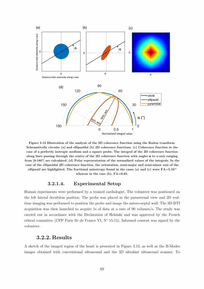
69

Figure 3.12 Illustration of the analysis of the 2D coherence function using the Radon transform. Schematically circular (a) and ellipsoidal (b) 2D coherence functions. (c) Coherence function in the case of a perfectly isotropic medium and a square probe. The integral of the 2D coherence function along lines passing through the centre of the 2D coherence function with angles α to x-axis ranging

from [0-180°[ are calculated. (d) Polar representation of the normalized values of the integrals. In the case of the ellipsoidal 2D coherence function, the orientation, semi-major and semi-minor axis of the

ellipsoid are highlighted. The fractional anisotropy found in the cases (a) and (c) were FA=5.10-4 whereas in the case (b), FA=0.65.

3.2.1.4. Experimental Setup Human experiments were performed by a trained cardiologist. The volunteer was positioned on the left lateral decubitus position. The probe was placed in the parasternal view and 2D real-time imaging was performed to position the probe and image the antero-septal wall. The 3D-BTI acquisition was then launched to acquire 1s of data at a rate of 90 volumes/s. The study was carried out in accordance with the Declaration of Helsinki and was approved by the French ethical committee (CPP Paris Ile de France VI, N° 15-15). Informed consent was signed by the volunteer.

3.2.2. Results A sketch of the imaged region of the heart is presented in Figure 3.13, as well as the B-Modes images obtained with conventional ultrasound and the 3D ultrafast ultrasound scanner. To

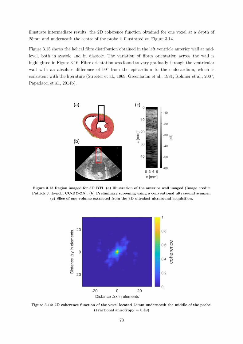
70

illustrate intermediate results, the 2D coherence function obtained for one voxel at a depth of 25mm and underneath the centre of the probe is illustrated on Figure 3.14.

Figure 3.15 shows the helical fibre distribution obtained in the left ventricle anterior wall at mid-level, both in systole and in diastole. The variation of fibres orientation across the wall is highlighted in Figure 3.16. Fibre orientation was found to vary gradually through the ventricular wall with an absolute difference of 99° from the epicardium to the endocardium, which is consistent with the literature (Streeter et al., 1969; Greenbaum et al., 1981; Rohmer et al., 2007; Papadacci et al., 2014b).

Figure 3.13 Region imaged for 3D BTI. (a) Illustration of the anterior wall imaged (Image credit: Patrick J. Lynch, CC-BY-2.5). (b) Preliminary screening using a conventional ultrasound scanner.

(c) Slice of one volume extracted from the 3D ultrafast ultrasound acquisition.

Figure 3.14: 2D coherence function of the voxel located 25mm underneath the middle of the probe. (Fractional anisotropy = 0.49)

71

Figure 3.15 Transthoracic imaging of myocardial fibre orientation in the human heart. (a) Angle definition with respect to LV: circumferential fibres have a 0° angle. Figure adapted from (Streeter et al., 1969). The orientations of the antero-septal LV wall fibres are shown in end-diastole (b) and end-

systole (c).

Figure 3.16 3D-BTI: Variations of angle across the cardiac wall thickness, in systole and diastole. To facilitate the comparison, the thickness of the wall in expressed in percentages.

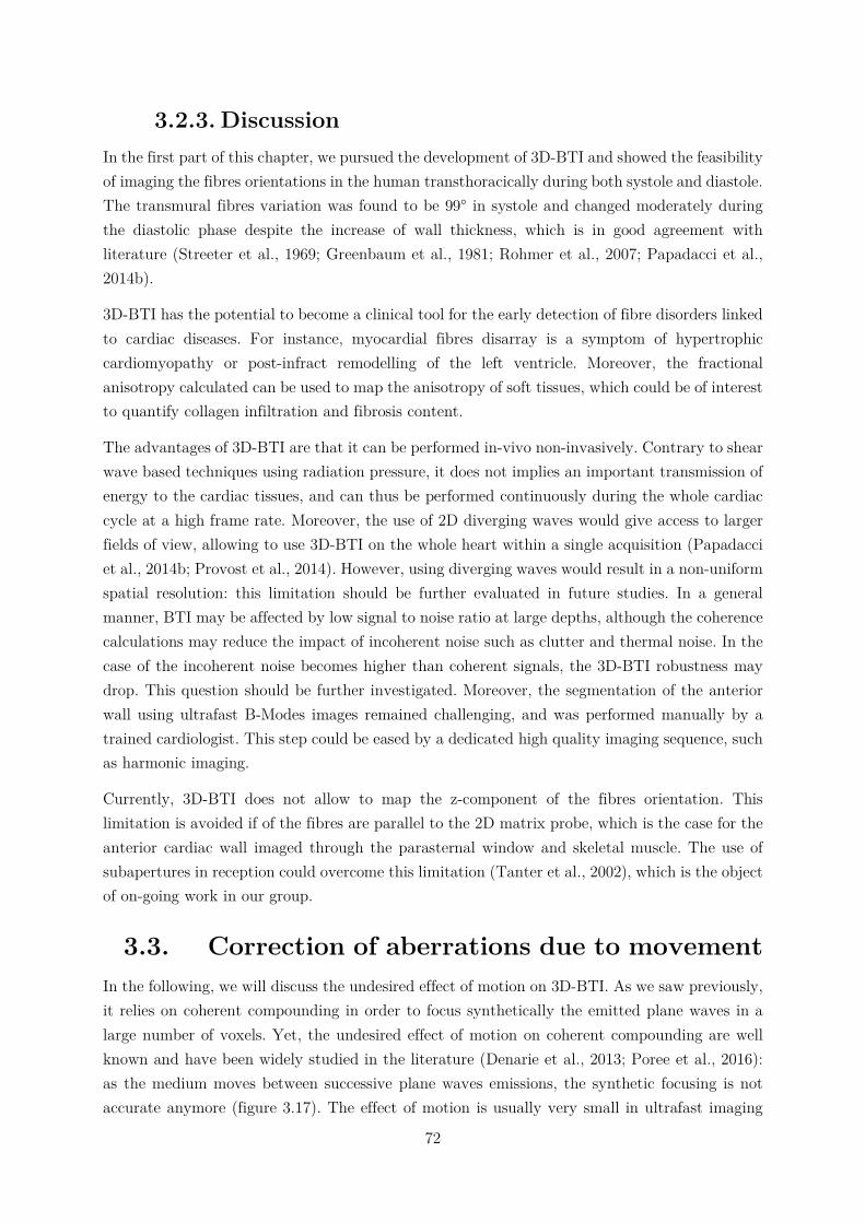
72

3.2.3. Discussion In the first part of this chapter, we pursued the development of 3D-BTI and showed the feasibility of imaging the fibres orientations in the human transthoracically during both systole and diastole. The transmural fibres variation was found to be 99° in systole and changed moderately during the diastolic phase despite the increase of wall thickness, which is in good agreement with literature (Streeter et al., 1969; Greenbaum et al., 1981; Rohmer et al., 2007; Papadacci et al., 2014b).

3D-BTI has the potential to become a clinical tool for the early detection of fibre disorders linked to cardiac diseases. For instance, myocardial fibres disarray is a symptom of hypertrophic cardiomyopathy or post-infract remodelling of the left ventricle. Moreover, the fractional anisotropy calculated can be used to map the anisotropy of soft tissues, which could be of interest to quantify collagen infiltration and fibrosis content.

The advantages of 3D-BTI are that it can be performed in-vivo non-invasively. Contrary to shear wave based techniques using radiation pressure, it does not implies an important transmission of energy to the cardiac tissues, and can thus be performed continuously during the whole cardiac cycle at a high frame rate. Moreover, the use of 2D diverging waves would give access to larger fields of view, allowing to use 3D-BTI on the whole heart within a single acquisition (Papadacci et al., 2014b; Provost et al., 2014). However, using diverging waves would result in a non-uniform spatial resolution: this limitation should be further evaluated in future studies. In a general manner, BTI may be affected by low signal to noise ratio at large depths, although the coherence calculations may reduce the impact of incoherent noise such as clutter and thermal noise. In the case of the incoherent noise becomes higher than coherent signals, the 3D-BTI robustness may drop. This question should be further investigated. Moreover, the segmentation of the anterior wall using ultrafast B-Modes images remained challenging, and was performed manually by a trained cardiologist. This step could be eased by a dedicated high quality imaging sequence, such as harmonic imaging.

Currently, 3D-BTI does not allow to map the z-component of the fibres orientation. This limitation is avoided if of the fibres are parallel to the 2D matrix probe, which is the case for the anterior cardiac wall imaged through the parasternal window and skeletal muscle. The use of subapertures in reception could overcome this limitation (Tanter et al., 2002), which is the object of on-going work in our group.

3.3. Correction of aberrations due to movement In the following, we will discuss the undesired effect of motion on 3D-BTI. As we saw previously, it relies on coherent compounding in order to focus synthetically the emitted plane waves in a large number of voxels. Yet, the undesired effect of motion on coherent compounding are well known and have been widely studied in the literature (Denarie et al., 2013; Poree et al., 2016): as the medium moves between successive plane waves emissions, the synthetic focusing is not accurate anymore (figure 3.17). The effect of motion is usually very small in ultrafast imaging

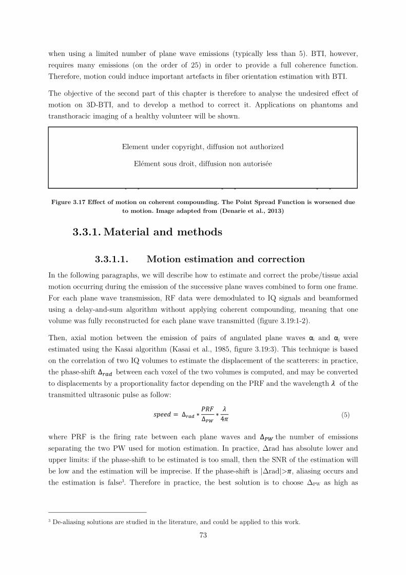
73

when using a limited number of plane wave emissions (typically less than 5). BTI, however, requires many emissions (on the order of 25) in order to provide a full coherence function. Therefore, motion could induce important artefacts in fiber orientation estimation with BTI.

The objective of the second part of this chapter is therefore to analyse the undesired effect of motion on 3D-BTI, and to develop a method to correct it. Applications on phantoms and transthoracic imaging of a healthy volunteer will be shown.

Figure 3.17 Effect of motion on coherent compounding. The Point Spread Function is worsened due to motion. Image adapted from (Denarie et al., 2013)


3.3.1.1. Motion estimation and correction In the following paragraphs, we will describe how to estimate and correct the probe/tissue axial motion occurring during the emission of the successive plane waves combined to form one frame. For each plane wave transmission, RF data were demodulated to IQ signals and beamformed using a delay-and-sum algorithm without applying coherent compounding, meaning that one volume was fully reconstructed for each plane wave transmitted (figure 3.19:1-2).

Then, axial motion between the emission of pairs of angulated plane waves αi and αj were estimated using the Kasai algorithm (Kasai et al., 1985, figure 3.19:3). This technique is based on the correlation of two IQ volumes to estimate the displacement of the scatterers: in practice, the phase-shift ∆ between each voxel of the two volumes is computed, and may be converted to displacements by a proportionality factor depending on the PRF and the wavelength 𝜆 of the transmitted ultrasonic pulse as follow:

𝑠𝑝𝑒𝑒𝑑 = ∆ ∗𝑃𝑅𝐹

∆∗

𝜆

4𝜋 (5)

where PRF is the firing rate between each plane waves and ∆ the number of emissions separating the two PW used for motion estimation. In practice, Δrad has absolute lower and upper limits: if the phase-shift to be estimated is too small, then the SNR of the estimation will be low and the estimation will be imprecise. If the phase-shift is |Δrad|>𝜋, aliasing occurs and the estimation is false3. Therefore in practice, the best solution is to choose ΔPW as high as

3 De-aliasing solutions are studied in the literature, and could be applied to this work.



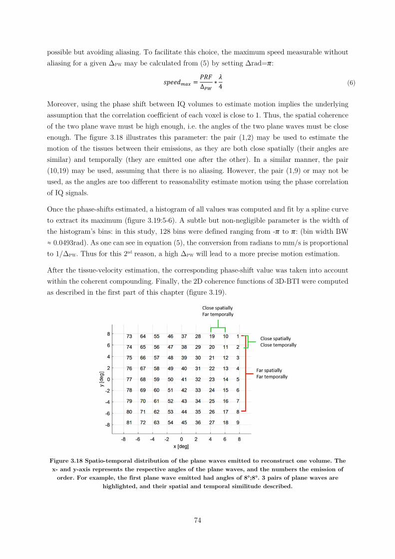
74

possible but avoiding aliasing. To facilitate this choice, the maximum speed measurable without aliasing for a given ΔPW may be calculated from (5) by setting Δrad=𝜋:

𝑠𝑝𝑒𝑒𝑑 =𝑃𝑅𝐹

∆∗

𝜆

4 (6)

Moreover, using the phase shift between IQ volumes to estimate motion implies the underlying assumption that the correlation coefficient of each voxel is close to 1. Thus, the spatial coherence of the two plane wave must be high enough, i.e. the angles of the two plane waves must be close enough. The figure 3.18 illustrates this parameter: the pair (1,2) may be used to estimate the motion of the tissues between their emissions, as they are both close spatially (their angles are similar) and temporally (they are emitted one after the other). In a similar manner, the pair (10,19) may be used, assuming that there is no aliasing. However, the pair (1,9) or may not be used, as the angles are too different to reasonability estimate motion using the phase correlation of IQ signals.

Once the phase-shifts estimated, a histogram of all values was computed and fit by a spline curve to extract its maximum (figure 3.19:5-6). A subtle but non-negligible parameter is the width of the histogram’s bins: in this study, 128 bins were defined ranging from -𝜋 to 𝜋: (bin width BW ≈ 0.0493rad). As one can see in equation (5), the conversion from radians to mm/s is proportional to 1/ΔPW. Thus for this 2nd reason, a high ΔPW will lead to a more precise motion estimation.

After the tissue-velocity estimation, the corresponding phase-shift value was taken into account within the coherent compounding. Finally, the 2D coherence functions of 3D-BTI were computed as described in the first part of this chapter (figure 3.19).

Figure 3.18 Spatio-temporal distribution of the plane waves emitted to reconstruct one volume. The x- and y-axis represents the respective angles of the plane waves, and the numbers the emission of

order. For example, the first plane wave emitted had angles of 8°;8°. 3 pairs of plane waves are highlighted, and their spatial and temporal similitude described.

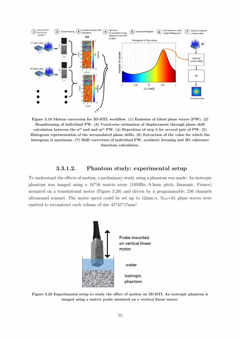
75

Figure 3.19 Motion correction for 3D-BTI: workflow. (1) Emission of tilted plane waves (PW). (2) Beamforming of individual PW. (3) Voxel-wise estimation of displacement through phase shift

calculation between the nth and and mth PW. (4) Repetition of step 3 for several pair of PW. (5) Histogram representation of the accumulated phase shifts. (6) Extraction of the value for which the histogram is maximum. (7) Shift correction of individual PW, synthetic focusing and 2D coherence

functions calculation.

3.3.1.2. Phantom study: experimental setup To understand the effects of motion, a preliminary study using a phantom was made. An isotropic phantom was imaged using a 16*16 matrix array (10MHz, 0.3mm pitch, Imasonic, France) mounted on a translational motor (Figure 3.20) and driven by a programmable, 256 channels ultrasound scanner. The motor speed could be set up to 12mm/s. NPW=81 plane waves were emitted to reconstruct each volume of size 45*45*17mm3.

Figure 3.20 Experimental setup to study the effect of motion on 3D-BTI. An isotropic phantom is imaged using a matrix probe mounted on a vertical linear motor.

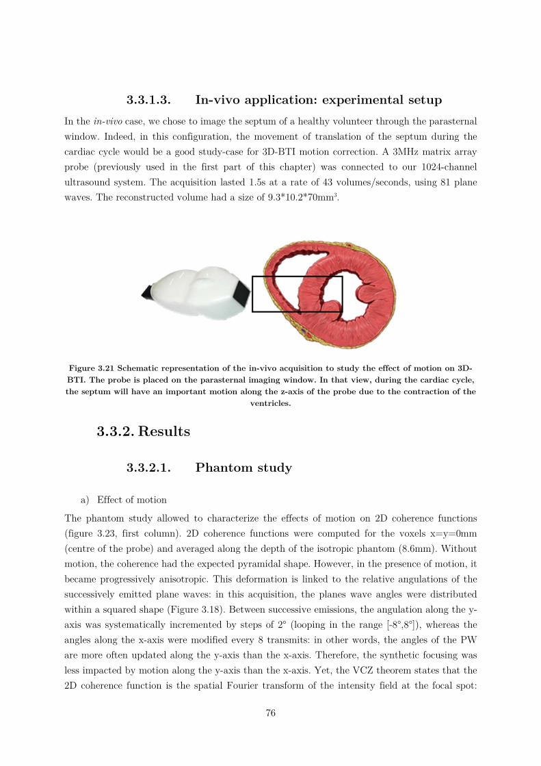
76

3.3.1.3. In-vivo application: experimental setup In the in-vivo case, we chose to image the septum of a healthy volunteer through the parasternal window. Indeed, in this configuration, the movement of translation of the septum during the cardiac cycle would be a good study-case for 3D-BTI motion correction. A 3MHz matrix array probe (previously used in the first part of this chapter) was connected to our 1024-channel ultrasound system. The acquisition lasted 1.5s at a rate of 43 volumes/seconds, using 81 plane waves. The reconstructed volume had a size of 9.3*10.2*70mm3.

Figure 3.21 Schematic representation of the in-vivo acquisition to study the effect of motion on 3D-BTI. The probe is placed on the parasternal imaging window. In that view, during the cardiac cycle, the septum will have an important motion along the z-axis of the probe due to the contraction of the

ventricles.

3.3.2. Results

3.3.2.1. Phantom study

a) Effect of motion

The phantom study allowed to characterize the effects of motion on 2D coherence functions (figure 3.23, first column). 2D coherence functions were computed for the voxels x=y=0mm (centre of the probe) and averaged along the depth of the isotropic phantom (8.6mm). Without motion, the coherence had the expected pyramidal shape. However, in the presence of motion, it became progressively anisotropic. This deformation is linked to the relative angulations of the successively emitted plane waves: in this acquisition, the planes wave angles were distributed within a squared shape (Figure 3.18). Between successive emissions, the angulation along the y-axis was systematically incremented by steps of 2° (looping in the range [-8°,8°]), whereas the angles along the x-axis were modified every 8 transmits: in other words, the angles of the PW are more often updated along the y-axis than the x-axis. Therefore, the synthetic focusing was less impacted by motion along the y-axis than the x-axis. Yet, the VCZ theorem states that the 2D coherence function is the spatial Fourier transform of the intensity field at the focal spot:

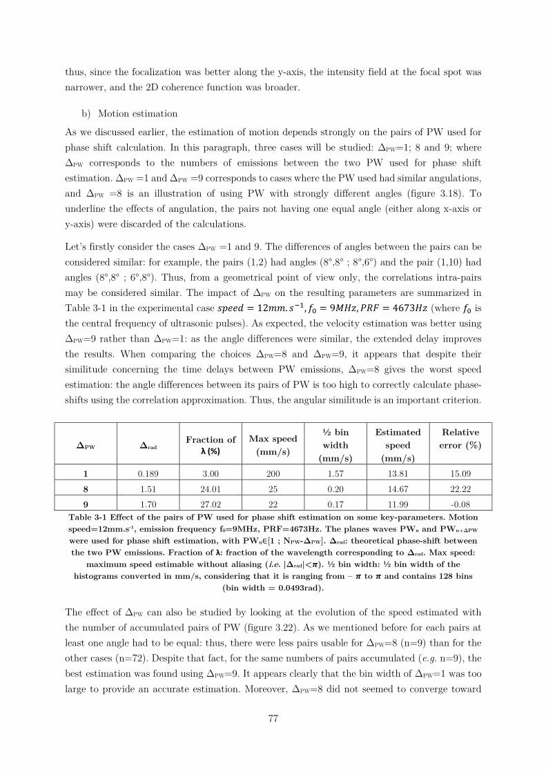
77

thus, since the focalization was better along the y-axis, the intensity field at the focal spot was narrower, and the 2D coherence function was broader.

b) Motion estimation

As we discussed earlier, the estimation of motion depends strongly on the pairs of PW used for phase shift calculation. In this paragraph, three cases will be studied: ΔPW=1; 8 and 9; where ΔPW corresponds to the numbers of emissions between the two PW used for phase shift estimation. ΔPW =1 and ΔPW =9 corresponds to cases where the PW used had similar angulations, and ΔPW =8 is an illustration of using PW with strongly different angles (figure 3.18). To underline the effects of angulation, the pairs not having one equal angle (either along x-axis or y-axis) were discarded of the calculations.

Let’s firstly consider the cases ΔPW =1 and 9. The differences of angles between the pairs can be considered similar: for example, the pairs (1,2) had angles (8°,8° ; 8°,6°) and the pair (1,10) had angles (8°,8° ; 6°,8°). Thus, from a geometrical point of view only, the correlations intra-pairs may be considered similar. The impact of ΔPW on the resulting parameters are summarized in Table 3-1 in the experimental case 𝑠𝑝𝑒𝑒𝑑 = 12𝑚𝑚. 𝑠 , 𝑓 = 9𝑀𝐻𝑧, 𝑃𝑅𝐹 = 4673𝐻𝑧 (where 𝑓 is the central frequency of ultrasonic pulses). As expected, the velocity estimation was better using ΔPW=9 rather than ΔPW=1: as the angle differences were similar, the extended delay improves the results. When comparing the choices ΔPW=8 and ΔPW=9, it appears that despite their similitude concerning the time delays between PW emissions, ΔPW=8 gives the worst speed estimation: the angle differences between its pairs of PW is too high to correctly calculate phase-shifts using the correlation approximation. Thus, the angular similitude is an important criterion.

ΔPW Δrad Fraction of

λ (%) Max speed

(mm/s)

½ bin width

(mm/s)

Estimated speed

(mm/s)

Relative error (%)

1 0.189 3.00 200 1.57 13.81 15.09 8 1.51 24.01 25 0.20 14.67 22.22 9 1.70 27.02 22 0.17 11.99 -0.08

Table 3-1 Effect of the pairs of PW used for phase shift estimation on some key-parameters. Motion speed=12mm.s-1, emission frequency f0=9MHz, PRF=4673Hz. The planes waves PWn and PWn+ΔPW were used for phase shift estimation, with PWn∈[1 ; NPW-ΔPW]. Δrad: theoretical phase-shift between the two PW emissions. Fraction of λ: fraction of the wavelength corresponding to Δrad. Max speed:

maximum speed estimable without aliasing (i.e. |Δrad|<𝝅). ½ bin width: ½ bin width of the histograms converted in mm/s, considering that it is ranging from – 𝝅 to 𝝅 and contains 128 bins

(bin width = 0.0493rad).

The effect of ΔPW can also be studied by looking at the evolution of the speed estimated with the number of accumulated pairs of PW (figure 3.22). As we mentioned before for each pairs at least one angle had to be equal: thus, there were less pairs usable for ΔPW=8 (n=9) than for the other cases (n=72). Despite that fact, for the same numbers of pairs accumulated (e.g. n=9), the best estimation was found using ΔPW=9. It appears clearly that the bin width of ΔPW=1 was too large to provide an accurate estimation. Moreover, ΔPW=8 did not seemed to converge toward

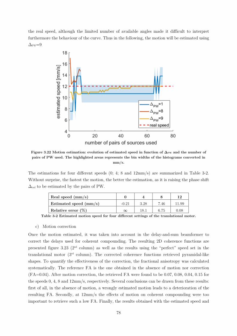
78

the real speed, although the limited number of available angles made it difficult to interpret furthermore the behaviour of the curve. Thus in the following, the motion will be estimated using ΔPW=9.

Figure 3.22 Motion estimation: evolution of estimated speed in function of ΔPW and the number of pairs of PW used. The highlighted areas represents the bin widths of the histograms converted in

mm/s.

The estimations for four different speeds (0; 4; 8 and 12mm/s) are summarized in Table 3-2. Without surprise, the fastest the motion, the better the estimation, as it is raising the phase shift Δrad to be estimated by the pairs of PW.

Real speed (mm/s) 0 4 8 12 Estimated speed (mm/s) -0.21 3.28 7.46 11.99 Relative error (%) ∞ 18.1 6.75 0.08

Table 3-2 Estimated motion speed for four different settings of the translational motor.

c) Motion correction

Once the motion estimated, it was taken into account in the delay-and-sum beamformer to correct the delays used for coherent compounding. The resulting 2D coherence functions are presented figure 3.23 (2nd column) as well as the results using the “perfect” speed set in the translational motor (3rd column). The corrected coherence functions retrieved pyramidal-like shapes. To quantify the effectiveness of the correction, the fractional anisotropy was calculated systematically. The reference FA is the one obtained in the absence of motion nor correction (FA=0.04). After motion correction, the retrieved FA were found to be 0.07, 0.08, 0.04, 0.15 for the speeds 0, 4, 8 and 12mm/s, respectively. Several conclusions can be drawn from these results: first of all, in the absence of motion, a wrongly estimated motion leads to a deterioration of the resulting FA. Secondly, at 12mm/s the effects of motion on coherent compounding were too important to retrieve such a low FA. Finally, the results obtained with the estimated speed and

79

the “real” speed were similar, indicating that the motion estimation was sufficiently precise to retrieve an isotropic coherence function. However, all the 2D coherence functions with motion correction were less spread than the reference image (i.e. no movement nor correction), which means according to the VCZ theorem that the intensity field at the focal spot was broader, so the synthetic focusing was degraded. Artefacts may be due to the approximation underlying the motion estimation using IQ phase-shifts and in that case, using RF correlations may improve the results. Despite this, in the context of fibre tracking, the FA was sufficiently lowered to consider the coherence functions (and thus the phantom) isotropic even in the presence of motion.

3.3.2.2. In-vivo study In this section, an in-vivo application of motion estimation and correction will be shown. A transthoracic ultrasound acquisition of the septum of a healthy volunteer was made through the parasternal window, and motion correction was applied on one frame during systole, when motion was substantial (27mm/s), but without aliasing. A posterori calculation of the equivalent phase shift using equation (5) gives Δrad=0.760rad, corresponding to 12.1% of the wavelength of the central ultrasound frequency. Thus, referring to the Table 3-1 in the phantom study section, we can suppose that the speed estimation error is below 15%.

To estimate the benefits of motion correction on 3D-BTI, the 2D coherence functions were calculated for each voxel in a region of interest of 4.4*4.8*9.0mm3, and a fibre tracking algorithm was then used to visualize the fibres orientations. Given the relatively small size of the reconstructed volumes, the fibres orientation were expected to be homogeneous at a given depth. It appeared that without correction, boundaries artefacts were present at the interfaces septum/blood (Figure 3.24). The angles distribution were more consistent with correction than without. This is better visualized when looking at the variation of angles over depth shown in figure 3.24c, where the average angles and the standard deviations at each depth of the 3D volumes are represented. With correction, the standard deviation was lower than without, indicating more homogeneous slices.

3.3.3. Discussion In the second part of this chapter, the effect of motion on 3D-BTI was studied. We proposed a methodology to estimate the axial motion, and correct its adverse effect on synthetic focusing, a fundamental step of 3D-BTI calculations. We saw that movement can deform 2D coherence functions: in the case of an isotropic medium, the distortion may lead to a misinterpretation of the degree of anisotropy of the region scanned. However, the velocity of tissues displacements may be estimated and accounted for within a frame with a limited number of PW, and we demonstrated that it was possible to retrieve isotropic 2D coherence functions in post-processing at a low computational cost. Yet, the deformations of coherence functions are directly related to the spatiotemporal distributions of tilted plane waves used for synthetic focusing. Therefore, a solution to reduce the motions artefacts would be to change the sequence of tilted plane waves

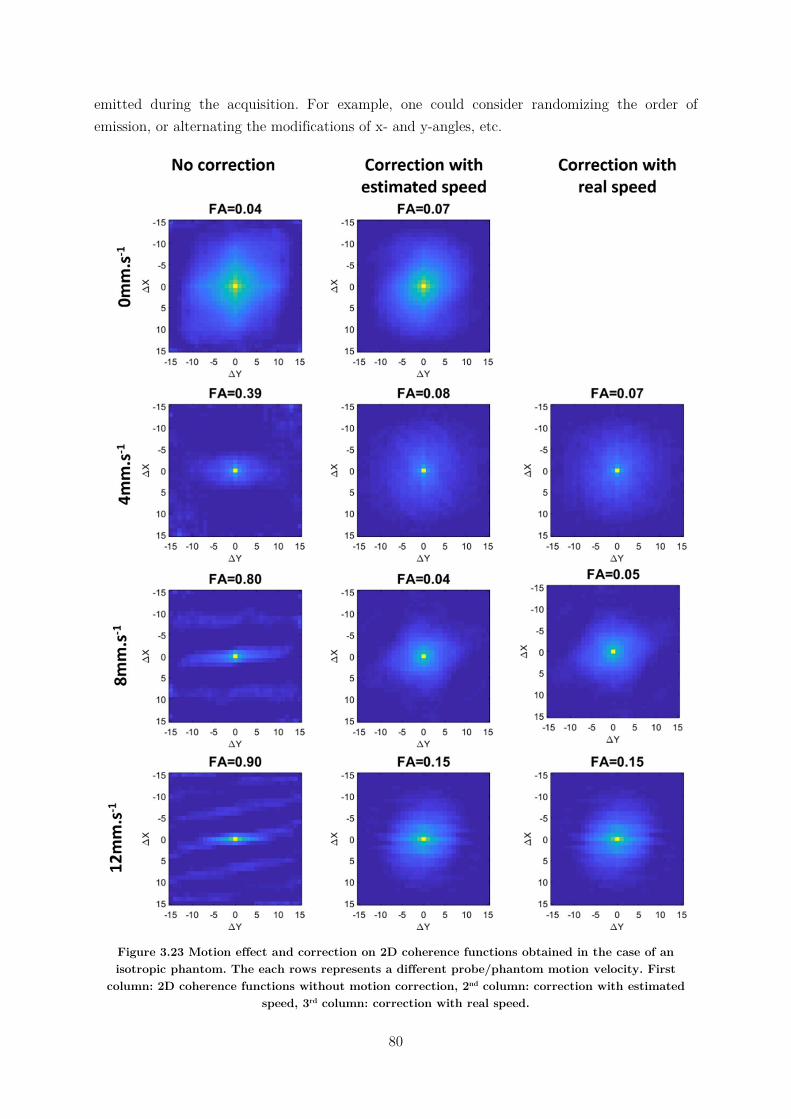
80

emitted during the acquisition. For example, one could consider randomizing the order of emission, or alternating the modifications of x- and y-angles, etc.

Figure 3.23 Motion effect and correction on 2D coherence functions obtained in the case of an isotropic phantom. The each rows represents a different probe/phantom motion velocity. First

column: 2D coherence functions without motion correction, 2nd column: correction with estimated speed, 3rd column: correction with real speed.

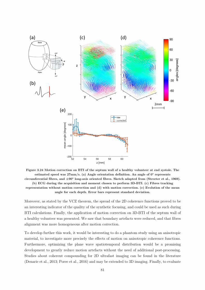
81

Figure 3.24 Motion correction on BTI of the septum wall of a healthy volunteer at end systole. The estimated speed was 27mm/s. (a) Angle orientation definition. An angle of 0° represents

circumferential fibres, and ±90° long-axis oriented fibres. Sketch adapted from (Streeter et al., 1969). (b) ECG during the acquisition and moment chosen to perform 3D-BTI. (c) Fibres tracking

representation without motion correction and (d) with motion correction. (e) Evolution of the mean angle for each depth. Error bars represent standard deviation.

Moreover, as stated by the VCZ theorem, the spread of the 2D coherence functions proved to be an interesting indicator of the quality of the synthetic focusing, and could be used as such during BTI calculations. Finally, the application of motion correction on 3D-BTI of the septum wall of a healthy volunteer was presented. We saw that boundary artefacts were reduced, and that fibres alignment was more homogeneous after motion correction.

To develop further this work, it would be interesting to do a phantom study using an anisotropic material, to investigate more precisely the effects of motion on anisotropic coherence functions. Furthermore, optimizing the plane wave spatiotemporal distribution would be a promising development to greatly reduce motion artefacts without the need of additional post-processing. Studies about coherent compounding for 2D ultrafast imaging can be found in the literature (Denarie et al., 2013; Poree et al., 2016) and may be extended to 3D imaging. Finally, to evaluate

82

the impact of motion for in-vivo applications, a study comparing results of 3D-BTI with and without motion correction and a ground truth (e.g. obtained by DTI or histology) would be interesting.

3.4. Conclusion In this chapter, we pursued the development of 3D-BTI toward a clinical setting. Applications on imaging the local fibres architecture of the antero-septal wall of the left ventricle of a healthy volunteer have been demonstrated at both end-systole and end-diastole. Despite the thickening of the heart during its contraction, no significant changes in angle variations through the wall has been noticed. Then, the undesired effects of motion on 3D-BTI have been studied: although important deformations of 2D coherence functions occurred, we saw that it was possible to estimate the velocity of axial motion and correct its adverse effects. Futures perspectives of this work will be the development of transmit sequences limiting motion artefact without the need of additional post-processing, which would allow to image the evolution of fibres orientation through the cardiac cycle with a sufficiently high SNR. Then, applications on cardiomyopathies would be interesting for the better understanding of the underlying mechanisms, the better follow-up of patients, and the early detection of cardiac abnormalities.

83


Arts, T., Costa, K.D., Covell, J.W., McCulloch, A.D., 2001. Relating myocardial laminar architecture to shear strain and muscle fiber orientation. Am. J. Physiol. Heart Circ. Physiol. 280, H2222-2229.

Baldwin, S.L., Marutyan, K.R., Yang, M., Wallace, K.D., Holland, M.R., Miller, J.G., 2006. Measurements of the anisotropy of ultrasonic attenuation in freshly excised myocardium. The Journal of the Acoustical Society of America 119, 3130. https://doi.org/10.1121/1.2188333

Bers, D., 2001. Excitation-Contraction Coupling and Cardiac Contractile Force. Springer Science & Business Media.

Correia, M., Deffieux, T., Chatelin, S., Provost, J., Tanter, M., Pernot, M., 2018. 3D elastic tensor imaging in weakly transversely isotropic soft tissues. Physics in Medicine & Biology 63, 155005. https://doi.org/10.1088/1361-6560/aacfaf

Correia, M.F.R., 2016. From 2D to 3D cardiovascular ultrafast ultrasound imaging : new insights in shear wave elastography and blood flow imaging.

Costa, K.D., Takayama, Y., McCulloch, A.D., Covell, J.W., 1999. Laminar fiber architecture and three-dimensional systolic mechanics in canine ventricular myocardium. Am. J. Physiol. 276, H595-607.

Dahl, J.J., Jakovljevic, M., Pinton, G.F., Trahey, G.E., 2012. Harmonic spatial coherence imaging: an ultrasonic imaging method based on backscatter coherence. IEEE Transactions on Ultrasonics, Ferroelectrics and Frequency Control 59, 648–659. https://doi.org/10.1109/TUFFC.2012.2243

Denarie, B., Tangen, T.A., Ekroll, I.K., Rolim, N., Torp, H., Bjastad, T., Lovstakken, L., 2013. Coherent Plane Wave Compounding for Very High Frame Rate Ultrasonography of Rapidly Moving Targets. IEEE Transactions on Medical Imaging 32, 1265–1276. https://doi.org/10.1109/TMI.2013.2255310

Derode, A., Fink, M., 1993. Spatial coherence of ultrasonic speckle in composites. IEEE Trans Ultrason Ferroelectr Freq Control 40, 666–675. https://doi.org/10.1109/58.248209

Fan, C., Yao, G., 2013. Imaging myocardial fiber orientation using polarization sensitive optical coherence tomography. Biomedical Optics Express 4, 460. https://doi.org/10.1364/BOE.4.000460

Fleming, C.P., Ripplinger, C.M., Webb, B., Efimov, I.R., Rollins, A.M., 2008. Quantification of cardiac fiber orientation using optical coherence tomography. J Biomed Opt 13, 030505. https://doi.org/10.1117/1.2937470

84

Fujimoto, J.G., Pitris, C., Boppart, S.A., Brezinski, M.E., 2000. Optical Coherence Tomography: An Emerging Technology for Biomedical Imaging and Optical Biopsy. Neoplasia 2, 9–25. https://doi.org/10.1038/sj.neo.7900071

Green, M.A., Geng, G., Qin, E., Sinkus, R., Gandevia, S.C., Bilston, L.E., 2013. Measuring anisotropic muscle stiffness properties using elastography: MEASURING ANISOTROPIC MUSCLE STIFFNESS PROPERTIES USING ELASTOGRAPHY. NMR in Biomedicine 26, 1387–1394. https://doi.org/10.1002/nbm.2964

Greenbaum, R.A., Ho, S.Y., Gibson, D.G., Becker, A.E., Anderson, R.H., 1981. Left ventricular fibre architecture in man. Heart 45, 248–263. https://doi.org/10.1136/hrt.45.3.248

Hansen, D.E., Daughters, G.T., Alderman, E.L., Ingels, N.B., Stinson, E.B., Miller, D.C., 1991. Effect of volume loading, pressure loading, and inotropic stimulation on left ventricular torsion in humans. Circulation 83, 1315–1326.

Hollman, K.W., Rigby, K.W., O’Donnell, M., 1999. Coherence factor of speckle from a multi-row probe. IEEE, pp. 1257–1260. https://doi.org/10.1109/ULTSYM.1999.849225

Hooks, D.A., Trew, M.L., Caldwell, B.J., Sands, G.B., LeGrice, I.J., Smaill, B.H., 2007. Laminar arrangement of ventricular myocytes influences electrical behavior of the heart. Circ. Res. 101, e103-112. https://doi.org/10.1161/CIRCRESAHA.107.161075

Hsu, E.W., Muzikant, A.L., Matulevicius, S.A., Penland, R.C., Henriquez, C.S., 1998. Magnetic resonance myocardial fiber-orientation mapping with direct histological correlation. Am. J. Physiol. 274, H1627-1634.

Huang, D., Swanson, E., Lin, C., Schuman, J., Stinson, W., Chang, W., Hee, M., Flotte, T., Gregory, K., Puliafito, C., et, al., 1991. Optical coherence tomography. Science 254, 1178–1181. https://doi.org/10.1126/science.1957169

Huang, H., Macgillivray, C., Kwon, H.-S., Lammerding, J., Robbins, J., Lee, R.T., So, P., 2009. Three-dimensional cardiac architecture determined by two-photon microtomy. J Biomed Opt 14, 044029. https://doi.org/10.1117/1.3200939

Imbault, M., Faccinetto, A., Osmanski, B.-F., Tissier, A., Deffieux, T., Gennisson, J.-L., Vilgrain, V., Tanter, M., 2017. Robust sound speed estimation for ultrasound-based hepatic steatosis assessment. Physics in Medicine and Biology 62, 3582–3598. https://doi.org/10.1088/1361-6560/aa6226

J G Mottley, J.G.M., 1990. Anisotropy of the ultrasonic attenuation in soft tissues: measurements in vitro. The Journal of the Acoustical Society of America 88, 1203–10. https://doi.org/10.1121/1.399751

Kadish, A., Shinnar, M., Moore, E.N., Levine, J.H., Balke, C.W., Spear, J.F., 1988. Interaction of fiber orientation and direction of impulse propagation with anatomic barriers in anisotropic canine myocardium. Circulation 78, 1478–1494.

85

Lediju, M.A., Trahey, G.E., Byram, B.C., Dahl, J.J., 2011. Short-lag spatial coherence of backscattered echoes: Imaging characteristics. IEEE transactions on ultrasonics, ferroelectrics, and frequency control 58.

Lee, W.-N., Pernot, M., Couade, M., Messas, E., Bruneval, P., Bel, A., Hagège, A.A., Fink, M., Tanter, M., 2012. Mapping myocardial fiber orientation using echocardiography-based shear wave imaging. IEEE Trans Med Imaging 31, 554–562. https://doi.org/10.1109/TMI.2011.2172690

Legrice, I., Hunter, P., Young, A., Smaill, B., 2001. The architecture of the heart: a data-based model. Philosophical Transactions of the Royal Society A: Mathematical, Physical and Engineering Sciences 359, 1217–1232. https://doi.org/10.1098/rsta.2001.0827

Madaras, E.I., Perez, J., Sobel, B.E., Mottley, J.G., Miller, J.G., 1988. Anisotropy of the ultrasonic backscatter of myocardial tissue: II. Measurements in vivo. J. Acoust. Soc. Am. 83, 762–769.

Mallart, R., Fink, M., 1994. Adaptive focusing in scattering media through sound‐speed inhomogeneities: The van Cittert Zernike approach and focusing criterion. The Journal of the Acoustical Society of America 96, 3721–3732. https://doi.org/10.1121/1.410562

Mallart, R., Fink, M., 1991. The van Cittert–Zernike theorem in pulse echo measurements. The Journal of the Acoustical Society of America 90, 2718–2727. https://doi.org/10.1121/1.401867

Nguyen, C.T., Dawkins, J., Bi, X., Marbán, E., Li, D., 2018. Diffusion Tensor Cardiac Magnetic Resonance Reveals Exosomes From Cardiosphere-Derived Cells Preserve Myocardial Fiber Architecture After Myocardial Infarction. JACC: Basic to Translational Science 3, 97–109. https://doi.org/10.1016/j.jacbts.2017.09.005

Özarslan, E., Vemuri, B.C., Mareci, T.H., 2005. Generalized scalar measures for diffusion MRI using trace, variance, and entropy: Generalized Scalar Measures for Diffusion MRI. Magnetic Resonance in Medicine 53, 866–876. https://doi.org/10.1002/mrm.20411

Pai-Chi Li, Meng-Lin Li, 2003. Adaptive imaging using the generalized coherence factor. IEEE Transactions on Ultrasonics, Ferroelectrics and Frequency Control 50, 128–141. https://doi.org/10.1109/TUFFC.2003.1182117

Papadacci, C., 2014. Imagerie échographique ultrarapide du cœur et des artères chez l’homme : Vers l’imagerie ultrarapide 3D et l’imagerie du tenseur de rétrodiffusion ultrasonore 141.

Papadacci, C., Finel, V., Provost, J., Villemain, O., Bruneval, P., Gennisson, J.-L., Tanter, M., Fink, M., Pernot, M., 2017. Imaging the dynamics of cardiac fiber orientation in vivo using 3D Ultrasound Backscatter Tensor Imaging. Scientific Reports 7. https://doi.org/10.1038/s41598-017-00946-7

86

Papadacci, C., Tanter, M., Pernot, M., Fink, M., 2014a. Ultrasound backscatter tensor imaging (BTI): analysis of the spatial coherence of ultrasonic speckle in anisotropic soft tissues. IEEE Trans Ultrason Ferroelectr Freq Control 61, 986–996. https://doi.org/10.1109/TUFFC.2014.2994

Papadacci, C., Tanter, M., Pernot, M., Fink, M., 2014b. Ultrasound backscatter tensor imaging (BTI): analysis of the spatial coherence of ultrasonic speckle in anisotropic soft tissues. IEEE Transactions on Ultrasonics, Ferroelectrics, and Frequency Control 61, 986–996. https://doi.org/10.1109/TUFFC.2014.2994

Poree, J., Posada, D., Hodzic, A., Tournoux, F., Cloutier, G., Garcia, D., 2016. High-Frame-Rate Echocardiography Using Coherent Compounding With Doppler-Based Motion-Compensation. IEEE Transactions on Medical Imaging 35, 1647–1657. https://doi.org/10.1109/TMI.2016.2523346


Qin, E.C., Sinkus, R., Geng, G., Cheng, S., Green, M., Rae, C.D., Bilston, L.E., 2013. Combining MR elastography and diffusion tensor imaging for the assessment of anisotropic mechanical properties: A phantom study. Journal of Magnetic Resonance Imaging 37, 217–226. https://doi.org/10.1002/jmri.23797

Reese, T.G., Weisskoff, R.M., Smith, R.N., Rosen, B.R., Dinsmore, R.E., Wedeen, V.J., 1995. Imaging myocardial fiber architecture in vivo with magnetic resonance. Magnetic resonance in medicine: official journal of the Society of Magnetic Resonance in Medicine / Society of Magnetic Resonance in Medicine 34, 786–791.

Roberts, D.E., Hersh, L.T., Scher, A.M., 1979. Influence of cardiac fiber orientation on wavefront voltage, conduction velocity, and tissue resistivity in the dog. Circ. Res. 44, 701–712.

Rohmer, D., Sitek, A., Gullberg, G.T., 2007. Reconstruction and Visualization of Fiber and Laminar Structure in the Normal Human Heart from Ex Vivo Diffusion Tensor Magnetic Resonance Imaging (DTMRI) Data: Investigative Radiology 42, 777–789. https://doi.org/10.1097/RLI.0b013e3181238330

Savadjiev, P., Strijkers, G.J., Bakermans, A.J., Piuze, E., Zucker, S.W., Siddiqi, K., 2012. Heart wall myofibers are arranged in minimal surfaces to optimize organ function. Proc. Natl. Acad. Sci. U.S.A. 109, 9248–9253. https://doi.org/10.1073/pnas.1120785109

Scollan, D.F., Holmes, A., Winslow, R., Forder, J., 1998. Histological validation of myocardial microstructure obtained from diffusion tensor magnetic resonance imaging. Am. J. Physiol. 275, H2308-2318.

87

Sinkus, R., Lorenzen, J., Schrader, D., Lorenzen, M., Dargatz, M., Holz, D., 2000. High-resolution tensor MR elastography for breast tumour detection. Physics in Medicine and Biology 45, 1649–1664. https://doi.org/10.1088/0031-9155/45/6/317

Sinkus, R., Tanter, M., Catheline, S., Lorenzen, J., Kuhl, C., Sondermann, E., Fink, M., 2005. Imaging anisotropic and viscous properties of breast tissue by magnetic resonance-elastography. Magnetic Resonance in Medicine 53, 372–387. https://doi.org/10.1002/mrm.20355

Streeter, D.D., Bassett, D.L., 1966. An engineering analysis of myocardial fiber orientation in pig’s left ventricle in systole. Anat. Rec. 155, 503–511. https://doi.org/10.1002/ar.1091550403

Streeter, D.D., Spotnitz, H.M., Patel, D.P., Ross, J., Sonnenblick, E.H., 1969. Fiber orientation in the canine left ventricle during diastole and systole. Circ. Res. 24, 339–347.

Svoboda, K., Yasuda, R., 2006. Principles of Two-Photon Excitation Microscopy and Its Applications to Neuroscience. Neuron 50, 823–839. https://doi.org/10.1016/j.neuron.2006.05.019

Taber, L.A., Yang, M., Podszus, W.W., 1996. Mechanics of ventricular torsion. J Biomech 29, 745–752.

Taccardi, B., Macchi, E., Lux, R.L., Ershler, P.R., Spaggiari, S., Baruffi, S., Vyhmeister, Y., 1994. Effect of myocardial fiber direction on epicardial potentials. Circulation 90, 3076–3090.

Tanter, M., Bercoff, J., Sandrin, L., Fink, M., 2002. Ultrafast compound imaging for 2-D motion vector estimation: application to transient elastography. IEEE Trans Ultrason Ferroelectr Freq Control 49, 1363–1374.

Tseng, W.-Y.I., Dou, J., Reese, T.G., Wedeen, V.J., 2006. Imaging myocardial fiber disarray and intramural strain hypokinesis in hypertrophic cardiomyopathy with MRI. Journal of Magnetic Resonance Imaging 23, 1–8. https://doi.org/10.1002/jmri.20473

Tseng, W.-Y.I., Reese, T.G., Weisskoff, R.M., Wedeen, V.J., 1999. Cardiac diffusion tensor MRI in vivo without strain correction. Magnetic Resonance in Medicine 42, 393–403. https://doi.org/10.1002/(SICI)1522-2594(199908)42:2<393::AID-MRM22>3.0.CO;2-F

Waldman, L.K., Nosan, D., Villarreal, F., Covell, J.W., 1988. Relation between transmural deformation and local myofiber direction in canine left ventricle. Circ. Res. 63, 550–562.

Walker, W.F., Trahey, G.E., 1997. Speckle coherence and implications for adaptive imaging. The Journal of the Acoustical Society of America 101, 1847–1858. https://doi.org/10.1121/1.418235

88

Wang, Y., Yao, G., 2013. Optical tractography of the mouse heart using polarization-sensitive optical coherence tomography. Biomedical Optics Express 4, 2540. https://doi.org/10.1364/BOE.4.002540

Wickline, S.A., Verdonk, E.D., Miller, J.G., 1991. Three-dimensional characterization of human ventricular myofiber architecture by ultrasonic backscatter. J. Clin. Invest. 88, 438–446. https://doi.org/10.1172/JCI115323

Wu, M.-T., Tseng, W.-Y.I., Su, M.-Y.M., Liu, C.-P., Chiou, K.-R., Wedeen, V.J., Reese, T.G., Yang, C.-F., 2006. Diffusion Tensor Magnetic Resonance Imaging Mapping the Fiber Architecture Remodeling in Human Myocardium After Infarction: Correlation With Viability and Wall Motion. Circulation 114, 1036–1045. https://doi.org/10.1161/CIRCULATIONAHA.105.545863

89

: 3D passive elastography

of the left ventricle

4. 3D passive elastography of the left ventricle ...................................................................... 89

4.1. Introduction ................................................................................................................. 90

4.1.1. Motivations: why myocardial stiffness is interesting ............................................ 90

4.1.2. State of the art: how to measure (myocardial) stiffness ....................................... 90

4.1.2.1. Premises of elastography ............................................................................... 90

4.1.2.2. Active Shear Wave Elastography ................................................................. 91

4.1.2.3. Passive Shear Wave Elastography ................................................................ 93

4.1.3. Objectives: non-invasive passive elastography ..................................................... 94

4.2. Material and methods .................................................................................................. 94

4.2.1. Simulation ............................................................................................................ 94

4.2.2. Ultrafast Ultrasound Imaging in-vivo ................................................................... 95

4.2.3. Post processing computation ................................................................................ 96

4.2.3.1. Computation of time-of-flight: correlation algorithm .................................... 96

4.2.3.2. Computation of distance travelled: fast marching algorithm ........................ 98

4.2.3.3. Computation of speed ................................................................................... 98

4.3. Results ......................................................................................................................... 99

4.3.1. Simulations ........................................................................................................... 99

4.3.2. In-vivo experiments .............................................................................................. 99

4.4. Discussion .................................................................................................................. 101

4.5. Conclusion ................................................................................................................. 106


90

3D passive elastography of the left

ventricle

4.1. Introduction

4.1.1. Motivations: why myocardial stiffness is

interesting The myocardium rigidity changes drastically during its contractions and relaxations, allowing for the effectiveness of blood circulation. Both systolic and diastolic stiffnesses are important parameters: the former is related to the strength of the heart, whereas the latter is linked the ability of cardiac chambers to refill before the next contraction. Abnormalities of myocardial stiffness are one of the key pathophysiological mechanisms of heart failure with preserved ejection fraction (Zile et al., 2004), play a major role in cardiomyopathies such as hypertrophic (Hoskins et al., 2010) or restrictive (Elliott et al., 2008; Kushwaha et al., 1997) cardiomyopathies, and are a good indicator to qualify ischemia (Pernot et al., 2016; Pislaru, 2004).

Today, however, non-invasive estimation of myocardial stiffness is challenging and the only validated tool to assess the ventricular stiffness in patients is pressure-volume loop measured by invasive cardiac catheterization. In this chapter, we will aim to develop a tool to measure the stiffness of the left ventricle during the cardiac cycle using a 4D ultrafast ultrasound scanner.

4.1.2. State of the art: how to measure (myocardial)

stiffness

4.1.2.1. Premises of elastography

Palpations

Elastography could be translated as “elasticity imaging”. In physics, elasticity is the ability of a solid to resist a distortion influenced by an external force or stress, and to return to its original shape once the external stimuli stops. Therefore, elastography consists of analysing the mechanical response of a medium to a mechanical stimuli.

The ancestor of elastography is the palpation, which has been known to be a relevant diagnosis tool since at least 1500BC. Palpations are still used today on a daily basis to assess the stiffness of bowels, breasts, wounds, tumours, etc. The development of imaging technologies improved the palpation by showing the strain induced by tissues: the clinicians may judge the stiffness of the tissues by more than a simple feeling underneath their hands and fingers. This technique has,

91

however, obvious restrictions: it is limited to accessible tissues, it is qualitative but not quantitative, and therefore operator dependent.

Quasi-static elastography

One of the first ultrasound elastography technique, quasi-static ultrasound elastography, was the straightforward evolution of manual palpation. Indeed, it is based on the comparison of the RF signals or B-Mode images obtained by pressing more or less the probe on the patients’ skin. Quasi-static elastography is still an active research field: developments of speckle-tracking benefits directly to this methodology, and clinical applications are being translated into commercial ultrasound systems (Varghese, 2009). The main limitations of this technique are the control of the stress applied, and the absence of quantification. In addition, it is limited to superficial organs, mainly the breast or the thyroid.

Assessing cardiac stiffness

When it comes to cardiac elasticity evaluation in the clinical setting, the most used technique is however the catheterization (Bonnet et al., 2017). It consists of the insertion of a device to measure both pressure and volume inside the left ventricle during the cardiac cycle. The plot of pressure against volume, commonly called PV loop, is full of information. In particular, the slopes 𝜕𝑃 𝜕𝑉⁄ at the end-systole and end-diastole points depict the responses of the volume to a sudden change of pressure, and has been linked to the elasticity of the myocardium (Burkhoff et al., 2005). Therefore, both systolic and diastolic elasticity can be evaluated. However, this technique has limitations: it gives a global estimation but not an image of elasticity: therefore, it may call for further analysis to localize the defective tissues. Furthermore, as any cardiac catheterization, it is highly invasive, risky, and time and money consuming. Therefore, non-invasive imaging techniques are expected to overcome PV loops limits in the future.

4.1.2.2. Active Shear Wave Elastography Non-invasive cardiac stiffness evaluation cannot rely on the mechanical stress applied on tissues because it is unknown in the myocardium. Therefore, it is not possible to directly deduce the elasticity of the myocardium by its displacement, strain, or other derived values. The solution came from the shear waves. Indeed, it is well known that the speed of such waves depends of the elastic properties of the medium in which they propagate. Using the knowledge of their speed is therefore an indirect way of sensing the rigidity of the propagation medium, which is a very convenient solution when the medium is hardly accessible, deformable, etc. For instance, seismology is widely based on the analysis of shear wave propagation. This technique has been translated to the analysis of shear waves travelling in the human body, and elastography is often referred as “human body seismology”. Shear Wave elastography (SWE), also called Shear Wave Imaging (SWI), that will be discussed below thus relies on the measurement of shear wave propagation speed to assess tissues elasticity.

92

a) MRI

MRI elastography uses vibrations typically below 500Hz generated by an external device, trigged and synchronized with the MR sequence. The excitation source may be a coil using the magnetic field of the MRI scanner, piezoelectric materials, or the coupling of a coil and a magnet in a similar way of acoustic speakers system. In the latter case, the device has to be put away from the main coil of the MRI scanner, and thus requires an additional component to transfer the vibrations induced to the tissues. The propagation of the shear waves is imaged using phase contrast MRI, and the elasticity properties of the tissues are obtained by inversions algorithms based on equations of motion. MRI elastography can be applied successfully to the liver, spleen, breast, skeletal muscle, brain, and heart. Cardiac PV loops and myocardial stiffness could successfully be retrieved on healthy volunteers (Elgeti et al., 2012; Robert et al., 2009; Wassenaar et al., 2016), and promising results have been shown on patients with diastolic function (Elgeti et al., 2014). However, cardiac MR elastography is not yet spread into the clinics, limited by the high cost and low availability of MR devices.

b) Ultrasound

Ultrasound echography can estimate tissue motion either in the axial dimension with a very good accuracy, or in all dimensions of the image using speckle-tracking algorithm, making it a tool of choice for elastography.

Shear wave elastography (SWE) using external sources

As discussed previously, elastography can also by performed by tracking shear waves propagating in the body. In the beginning of ultrasound shear wave elastography, vibrations were induced by an external device: for example, Catheline et al attached an actuator to a 1D ultrasound transducer. By sending a pulse to the actuator, a spherical shear wave was generated in the tissues and its axial velocity could be estimated using the ultrasound transducer (Catheline, 1998). This simple technology proved to be able to retrieve the stiffness of the scanned tissues and led to the creation of the Echosens company, with is commercializing a device to quantify the hepatic fibrosis by elastography. Later, the actuator was mounted on a linear probe, allowing for 2D elastography. As shear wave propagates at several meters per seconds, a very high framerate (several thousand of frame per seconds) was required to image the shear wave propagation: ultrafast ultrasound imaging with plane waves was developed for this purpose (Sandrin et al., 1999). Applications on breast cancer detection was successfully shown (Bercoff et al., 2003).

Shear wave elastography using internal sources induced remotely

A major development of ultrasound elastography was led by the possibility to create shear waves inside the tissues without the use of external actuators, thus simplifying greatly the device. Indeed, when focalizing an ultrasound beam in a medium, the matter at the focal spot is slightly pushed by the acoustic radiation force according to Hooke’s law. When the pushing force is released, the matter comes back to its original position, thus creating a shear wave propagation in the surrounding medium perpendicularly to the ultrasonic beam. This idea of using acoustic

93

radiation force to remotely induced shear waves was developed in the 1990s (Sugimoto et al., 1990; Nightingale et al., 2001; Sarvazyan et al., 1998). In the beginning of the 00s, Bercoff et al. introduced a methodology to generate a shear wave Mach cone by moving the focal spot of the pushing beam (Bercoff et al., 2002). By doing this, plane shear waves could be generated in the tissues and propagated in a wider area without increasing the amplitude of the shear waves (which could be dangerous for the tissues), nor repeating ultrasonic pushes (which would increase proportionally the acquisition time). This technique has allowed quantitative imaging of soft tissues such as the breast, the liver or the thyroid and is now widely used in the clinics for diagnostic (Berg et al., 2012; Sebag et al., 2010).

Applications to cardiac elastography

Cardiac SWE has been successfully applied to measure the stiffness of the myocardium during the cardiac cycle on isolated rat hearts (Pernot et al., 2011), on healthy volunteers (Song et al., 2013), paediatric healthy volunteer as well as in patients with hypertrophic cardiomyopathy (Song et al., 2016; Villemain et al., 2018a, 2018b), and proved to be able to distinguish sunned or infracted myocardium (Pernot et al., 2016).

SWE presents however several technical limitations for cardiac applications. Indeed, to generate a shear wave the ultrasonic push has to be orthogonal to the myocardium. This can be obtained clinically only through the parasternal window, thus limiting the number of myocardial segments that can be reached. Moreover, the shear waves generated by SWE are strongly attenuated in the heart walls. Quantification of the entire or at least a large part of the left ventricle would require to generate shear waves of high amplitude which is not possible by the acoustic radiation force because of acoustic power safety limitations. Moreover, it requires imaging the shear wave propagation in 3D at high volume rate.

4.1.2.3. Passive Shear Wave Elastography Unlike active elastography, passive elastography relies on the imaging of elastic waves generated naturally by the body. The propagation of such natural elastic waves in the myocardium at different time points of the cardiac cycle has been investigated extensively (Kanai, 2005; Pernot et al., 2007). Several elastic waves have been identified as shear or lamb waves created by valve closures such as the aortic valve clap which is a strong mechanical source of sound and vibration in the heart. Other mechanical events are linked to active contraction events in the cardiac cycle such as the atrial and ventricular contractions. The propagation of these elastic waves has been imaged with ultrafast imaging in order to quantify their velocity (Papadacci et al., 2014; Provost et al., 2011; Vos et al., 2017).

Furthermore, correlation of noise-like elastic waves generated by remote organs, breathing, or muscle noise can also be used to retrieve stiffness properties of soft tissues without the need of a strong source of vibrations: applications on skeletal muscle (Sabra et al., 2007), liver (Gallot et al., 2011) or thyroid (Catheline et al., 2013) etc. have been showed.

94

2D ultrafast imaging remains however too limited to image the wave propagation in a tridimensional structure such as the ventricle.

4.1.3. Objectives: non-invasive passive elastography In this chapter, we aim to image non-invasively and in 3D the velocity of natural elastic waves propagating along the left ventricle wall during both systole and diastole. Indeed, the closure of the aortic valve at the end of the systole is a strong mechanical event responsible for the 2nd heart sound, and generating a elastic wave propagating in the left ventricle, when it is contracted. Interestingly, when the atrium contracts to eject blood in the left ventricle (the atrial kick), an elastic wave propagating is also visible, and can be exploited to assess the diastolic stiffness of the LV.

The objectives of the study are 1) to establish a methodology for 3D mapping of the left ventricular stiffness, 2) to validate its accuracy using finite differences simulations and 3) to show the in vivo feasibility on the hearts of healthy volunteer.

4.2. Material and methods

4.2.1. Simulation Synthetic elastic wave propagation data were generated to investigate the accuracy of our method. End-diastole and end-systole 3D ellipsoidal models of the left ventricle (LV) were defined from (van den Broek and van den Broek, 1980). The model consisted of two truncated ellipsoids defining the endocardium and the epicardium according to the equation:

𝒙𝟐

𝒃𝟐+

𝒚𝟐

𝒃𝟐+

𝒛𝟐

𝒂𝟐= 𝟏

where a and b are the semi-long and semi-short axes of the ellipsoid, respectively. The ellipsoids were truncated at the intersection with the plane 𝑧 = 𝑘𝑎. The parameters 𝑎, 𝑏 and 𝑘 are defined in Table 4-1.

The elastic wave propagation was then simulated using the k-Wave toolbox for Matlab (Treeby et al., 2014) (figure 1a). A velocity point-source (1 cycle at 50Hz with hanning apodization) was placed at the base of the LV to simulate the effect of a mechanical source close to the aortic valve or the atrium. 3D visco-elastic kwave simulations (Treeby et al., 2014) were run for different shear wave velocity parameter: 1-2-3m/s for the diastole geometry and 4-5-6m/s for systole geometry, in order to cover a wide range of speeds observable in-vivo. The main simulation parameters are summarized in Table 4-1.

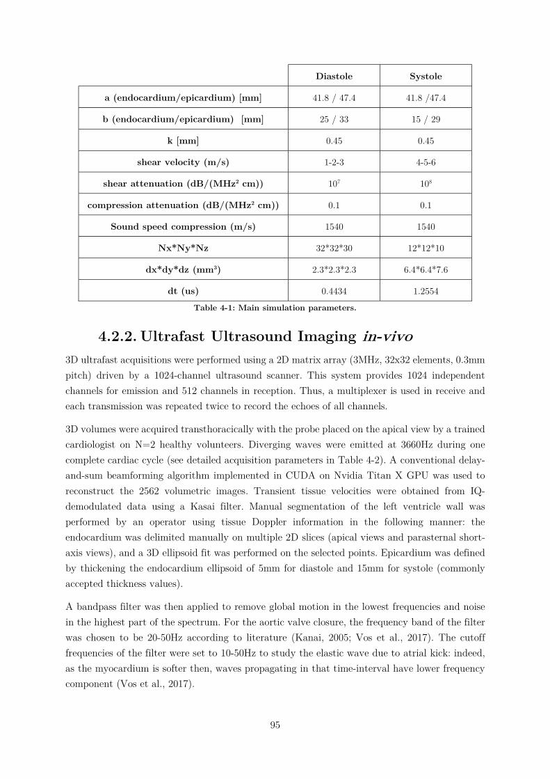
95

Diastole Systole

a (endocardium/epicardium) [mm] 41.8 / 47.4 41.8 /47.4

b (endocardium/epicardium) [mm] 25 / 33 15 / 29

k [mm] 0.45 0.45

shear velocity (m/s) 1-2-3 4-5-6

shear attenuation (dB/(MHz2 cm)) 107 108

compression attenuation (dB/(MHz2 cm)) 0.1 0.1

Sound speed compression (m/s) 1540 1540

Nx*Ny*Nz 32*32*30 12*12*10

dx*dy*dz (mm3) 2.3*2.3*2.3 6.4*6.4*7.6

dt (us) 0.4434 1.2554

Table 4-1: Main simulation parameters.

4.2.2. Ultrafast Ultrasound Imaging in-vivo 3D ultrafast acquisitions were performed using a 2D matrix array (3MHz, 32x32 elements, 0.3mm pitch) driven by a 1024-channel ultrasound scanner. This system provides 1024 independent channels for emission and 512 channels in reception. Thus, a multiplexer is used in receive and each transmission was repeated twice to record the echoes of all channels.

3D volumes were acquired transthoracically with the probe placed on the apical view by a trained cardiologist on N=2 healthy volunteers. Diverging waves were emitted at 3660Hz during one complete cardiac cycle (see detailed acquisition parameters in Table 4-2). A conventional delay-and-sum beamforming algorithm implemented in CUDA on Nvidia Titan X GPU was used to reconstruct the 2562 volumetric images. Transient tissue velocities were obtained from IQ-demodulated data using a Kasai filter. Manual segmentation of the left ventricle wall was performed by an operator using tissue Doppler information in the following manner: the endocardium was delimited manually on multiple 2D slices (apical views and parasternal short-axis views), and a 3D ellipsoid fit was performed on the selected points. Epicardium was defined by thickening the endocardium ellipsoid of 5mm for diastole and 15mm for systole (commonly accepted thickness values).

A bandpass filter was then applied to remove global motion in the lowest frequencies and noise in the highest part of the spectrum. For the aortic valve closure, the frequency band of the filter was chosen to be 20-50Hz according to literature (Kanai, 2005; Vos et al., 2017). The cutoff frequencies of the filter were set to 10-50Hz to study the elastic wave due to atrial kick: indeed, as the myocardium is softer then, waves propagating in that time-interval have lower frequency component (Vos et al., 2017).

96

Eventually, the 3D data were spatially smoothed by a convolution filter (kernel size of 3.9*3.9*3.2mm3).

Analysis of the shear wave propagation were performed on 60ms-long windows centred on the maximum of amplitude of transient displacements due to each event.

4.2.3. Post processing computation The post-processing workflow was divided into 3 main parts: 1. Localization of the source of the wave and computation of time-of-flight map, 2. Computation of distances from the source to the rest of the ventricle, 3. Combination of distances and time-of-flight maps to obtain speed map.

4.2.3.1. Computation of time-of-flight: correlation

algorithm First of all, the localization of the wave’s source was identified manually on 4D transient velocity movies by the operator (figure 4.1 a1 to a3), and N=10 reference points in the myocardium were randomly chosen within a 10mm radius from the source.

Time correlations of transient velocities between the N reference points and the rest of myocardium were performed. The correlation coefficients as well as the corresponding time shifts were stored. To average these N correlations, all the time shifts were lagged so that the first reference points had a time shift equals to 0ms on all maps. Then, the time maps were averaged using weights given by the correlation coefficients. Finally, the resulting time map was shifted so the activation time t0 of the source point is equal to 0ms (Figure 4.1d).

For the in-vivo situation only, the tissue Doppler energy and the mean coefficient of correlation over the N repetitions of calculations were used to apply thresholds. The points with an average correlation coefficient below 0.5 or an energy (normalized by the energy of the source) below -10dB were discarded (Figure 4.1b and Figure 4.1c). These steps allowed to insure that the results integrated only the region where the shear wave actually propagated and that the signal-to-noise ratio of individual voxels was high enough to be relevant, respectively.

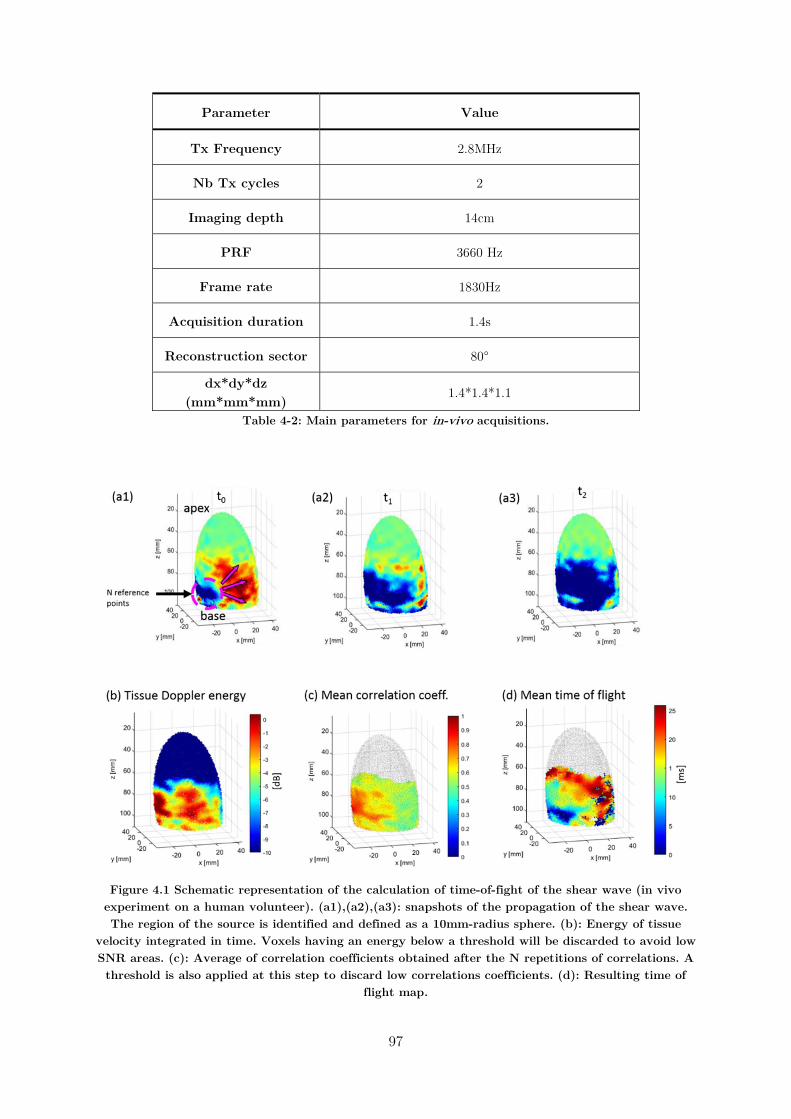
97

Parameter Value

Tx Frequency 2.8MHz

Nb Tx cycles 2

Imaging depth 14cm

PRF 3660 Hz

Frame rate 1830Hz

Acquisition duration 1.4s

Reconstruction sector 80°

dx*dy*dz (mm*mm*mm)

1.4*1.4*1.1

Table 4-2: Main parameters for in-vivo acquisitions.

Figure 4.1 Schematic representation of the calculation of time-of-fight of the shear wave (in vivo experiment on a human volunteer). (a1),(a2),(a3): snapshots of the propagation of the shear wave. The region of the source is identified and defined as a 10mm-radius sphere. (b): Energy of tissue

velocity integrated in time. Voxels having an energy below a threshold will be discarded to avoid low SNR areas. (c): Average of correlation coefficients obtained after the N repetitions of correlations. A threshold is also applied at this step to discard low correlations coefficients. (d): Resulting time of

flight map.

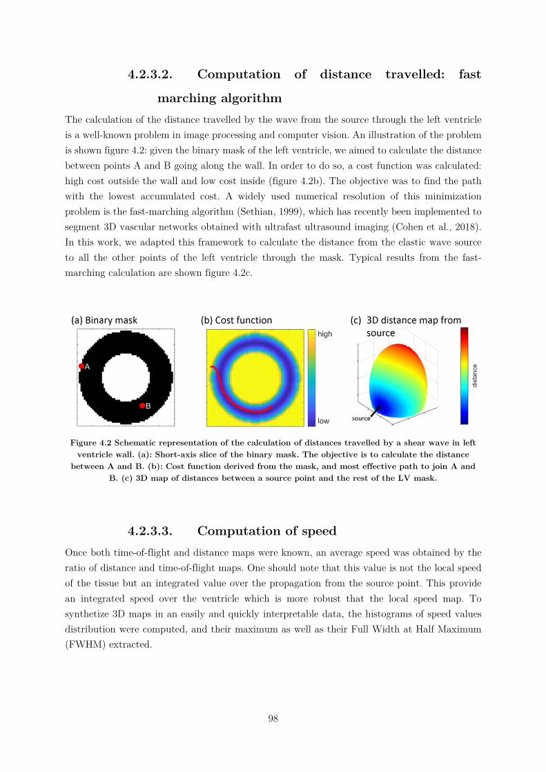
98

4.2.3.2. Computation of distance travelled: fast

marching algorithm The calculation of the distance travelled by the wave from the source through the left ventricle is a well-known problem in image processing and computer vision. An illustration of the problem is shown figure 4.2: given the binary mask of the left ventricle, we aimed to calculate the distance between points A and B going along the wall. In order to do so, a cost function was calculated: high cost outside the wall and low cost inside (figure 4.2b). The objective was to find the path with the lowest accumulated cost. A widely used numerical resolution of this minimization problem is the fast-marching algorithm (Sethian, 1999), which has recently been implemented to segment 3D vascular networks obtained with ultrafast ultrasound imaging (Cohen et al., 2018). In this work, we adapted this framework to calculate the distance from the elastic wave source to all the other points of the left ventricle through the mask. Typical results from the fast-marching calculation are shown figure 4.2c.

Figure 4.2 Schematic representation of the calculation of distances travelled by a shear wave in left ventricle wall. (a): Short-axis slice of the binary mask. The objective is to calculate the distance

between A and B. (b): Cost function derived from the mask, and most effective path to join A and B. (c) 3D map of distances between a source point and the rest of the LV mask.

4.2.3.3. Computation of speed Once both time-of-flight and distance maps were known, an average speed was obtained by the ratio of distance and time-of-flight maps. One should note that this value is not the local speed of the tissue but an integrated value over the propagation from the source point. This provide an integrated speed over the ventricle which is more robust that the local speed map. To synthetize 3D maps in an easily and quickly interpretable data, the histograms of speed values distribution were computed, and their maximum as well as their Full Width at Half Maximum (FWHM) extracted.

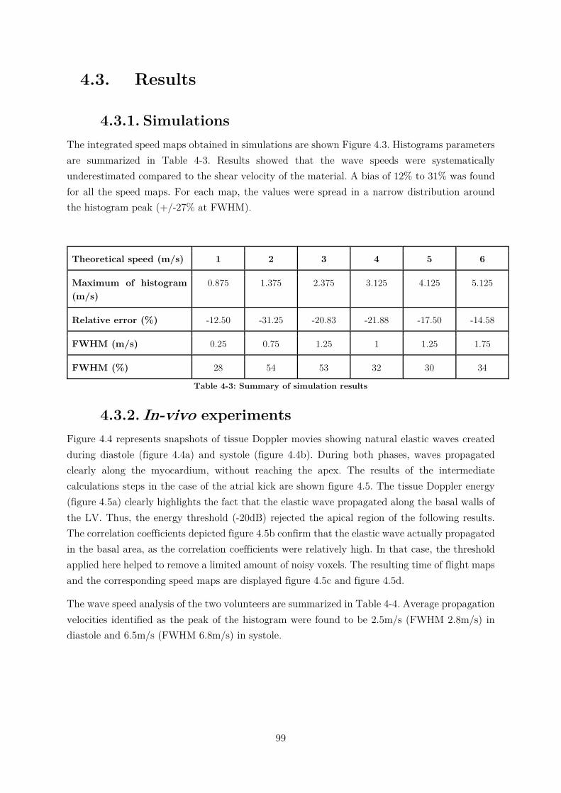
99

4.3. Results

4.3.1. Simulations The integrated speed maps obtained in simulations are shown Figure 4.3. Histograms parameters are summarized in Table 4-3. Results showed that the wave speeds were systematically underestimated compared to the shear velocity of the material. A bias of 12% to 31% was found for all the speed maps. For each map, the values were spread in a narrow distribution around the histogram peak (+/-27% at FWHM).

Theoretical speed (m/s) 1 2 3 4 5 6

Maximum of histogram (m/s)

0.875 1.375 2.375 3.125 4.125 5.125

Relative error (%) -12.50 -31.25 -20.83 -21.88 -17.50 -14.58

FWHM (m/s) 0.25 0.75 1.25 1 1.25 1.75

FWHM (%) 28 54 53 32 30 34

Table 4-3: Summary of simulation results

4.3.2. In-vivo experiments Figure 4.4 represents snapshots of tissue Doppler movies showing natural elastic waves created during diastole (figure 4.4a) and systole (figure 4.4b). During both phases, waves propagated clearly along the myocardium, without reaching the apex. The results of the intermediate calculations steps in the case of the atrial kick are shown figure 4.5. The tissue Doppler energy (figure 4.5a) clearly highlights the fact that the elastic wave propagated along the basal walls of the LV. Thus, the energy threshold (-20dB) rejected the apical region of the following results. The correlation coefficients depicted figure 4.5b confirm that the elastic wave actually propagated in the basal area, as the correlation coefficients were relatively high. In that case, the threshold applied here helped to remove a limited amount of noisy voxels. The resulting time of flight maps and the corresponding speed maps are displayed figure 4.5c and figure 4.5d.

The wave speed analysis of the two volunteers are summarized in Table 4-4. Average propagation velocities identified as the peak of the histogram were found to be 2.5m/s (FWHM 2.8m/s) in diastole and 6.5m/s (FWHM 6.8m/s) in systole.

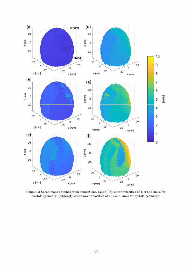
100

Figure 4.3 Speed maps obtained from simulations. (a),(b),(c): shear velocities of 1, 2 and 3m/s for diastole geometry. (d),(e),(f): shear wave velocities of 4, 5 and 6m/s for systole geometry.

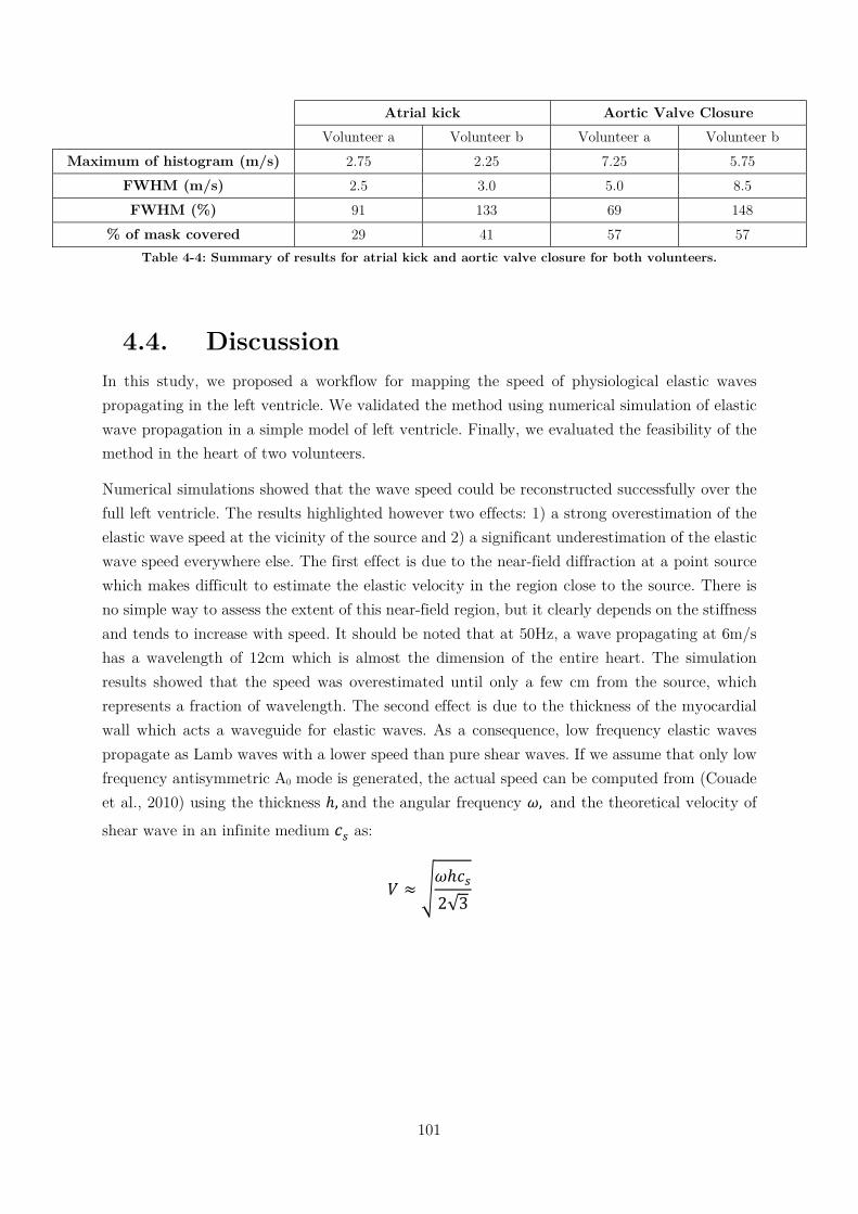
101

Atrial kick Aortic Valve Closure Volunteer a Volunteer b Volunteer a Volunteer b

Maximum of histogram (m/s) 2.75 2.25 7.25 5.75 FWHM (m/s) 2.5 3.0 5.0 8.5 FWHM (%) 91 133 69 148

% of mask covered 29 41 57 57 Table 4-4: Summary of results for atrial kick and aortic valve closure for both volunteers.

4.4. Discussion In this study, we proposed a workflow for mapping the speed of physiological elastic waves propagating in the left ventricle. We validated the method using numerical simulation of elastic wave propagation in a simple model of left ventricle. Finally, we evaluated the feasibility of the method in the heart of two volunteers.

Numerical simulations showed that the wave speed could be reconstructed successfully over the full left ventricle. The results highlighted however two effects: 1) a strong overestimation of the elastic wave speed at the vicinity of the source and 2) a significant underestimation of the elastic wave speed everywhere else. The first effect is due to the near-field diffraction at a point source which makes difficult to estimate the elastic velocity in the region close to the source. There is no simple way to assess the extent of this near-field region, but it clearly depends on the stiffness and tends to increase with speed. It should be noted that at 50Hz, a wave propagating at 6m/s has a wavelength of 12cm which is almost the dimension of the entire heart. The simulation results showed that the speed was overestimated until only a few cm from the source, which represents a fraction of wavelength. The second effect is due to the thickness of the myocardial wall which acts a waveguide for elastic waves. As a consequence, low frequency elastic waves propagate as Lamb waves with a lower speed than pure shear waves. If we assume that only low frequency antisymmetric A0 mode is generated, the actual speed can be computed from (Couade et al., 2010) using the thickness ℎ, and the angular frequency 𝜔, and the theoretical velocity of

shear wave in an infinite medium 𝑐𝑠 as:

𝑉 ≈𝜔ℎ𝑐

2√3

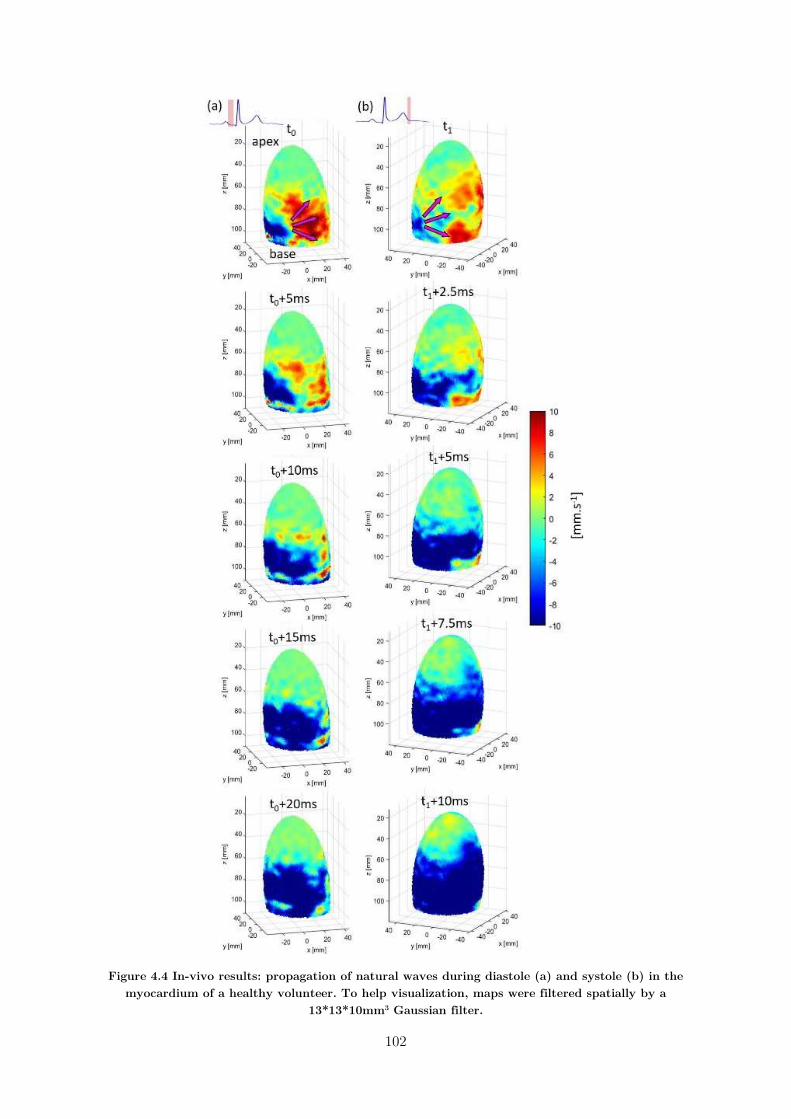
102

Figure 4.4 In-vivo results: propagation of natural waves during diastole (a) and systole (b) in the myocardium of a healthy volunteer. To help visualization, maps were filtered spatially by a

13*13*10mm3 Gaussian filter.

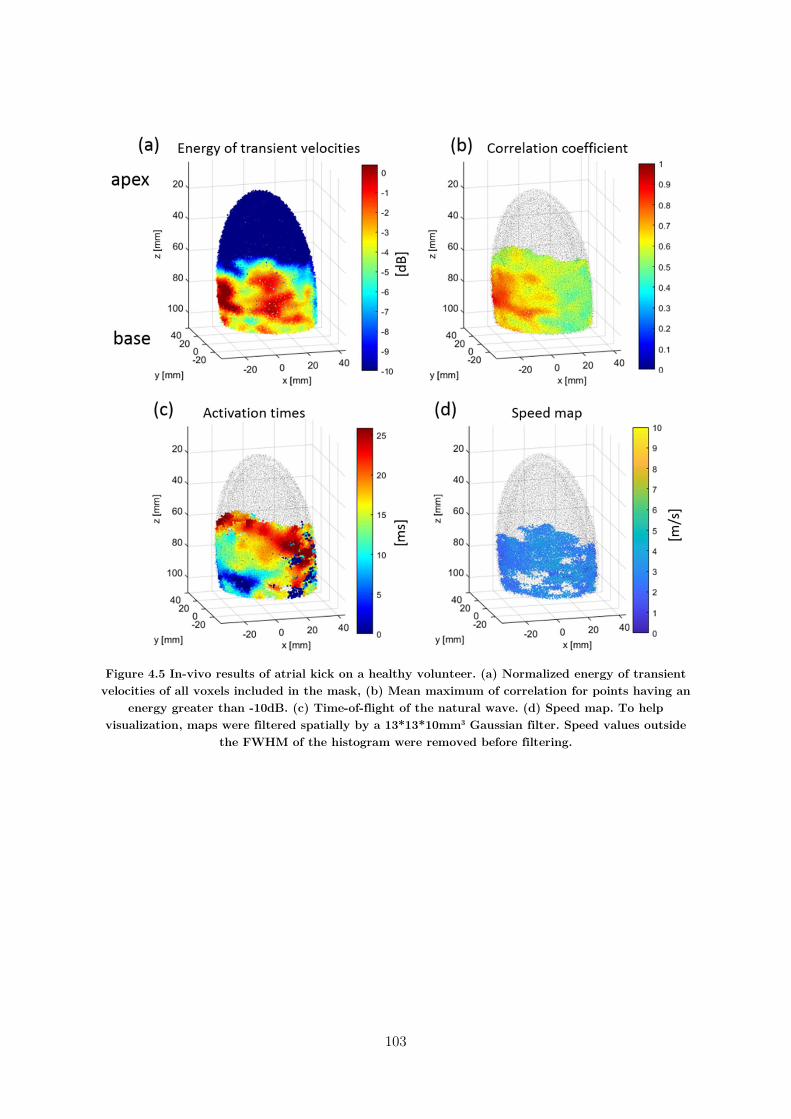
103

Figure 4.5 In-vivo results of atrial kick on a healthy volunteer. (a) Normalized energy of transient velocities of all voxels included in the mask, (b) Mean maximum of correlation for points having an

energy greater than -10dB. (c) Time-of-flight of the natural wave. (d) Speed map. To help visualization, maps were filtered spatially by a 13*13*10mm3 Gaussian filter. Speed values outside

the FWHM of the histogram were removed before filtering.

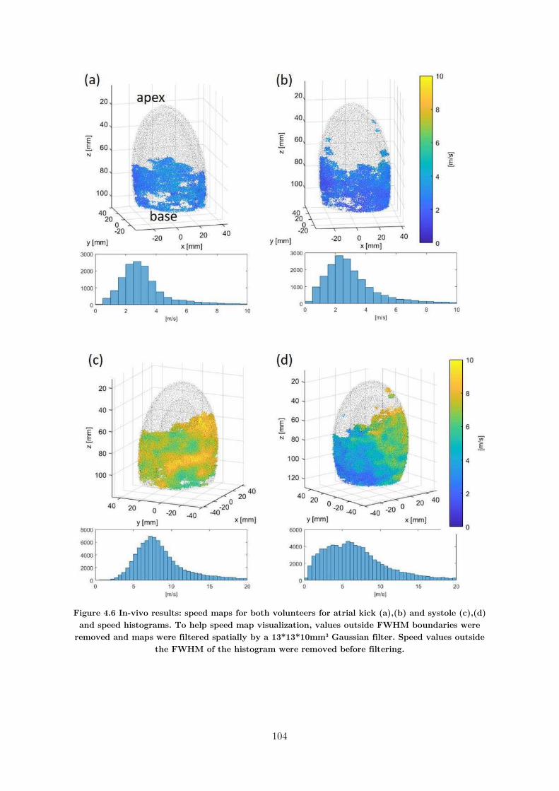
104

Figure 4.6 In-vivo results: speed maps for both volunteers for atrial kick (a),(b) and systole (c),(d) and speed histograms. To help speed map visualization, values outside FWHM boundaries were

removed and maps were filtered spatially by a 13*13*10mm3 Gaussian filter. Speed values outside the FWHM of the histogram were removed before filtering.

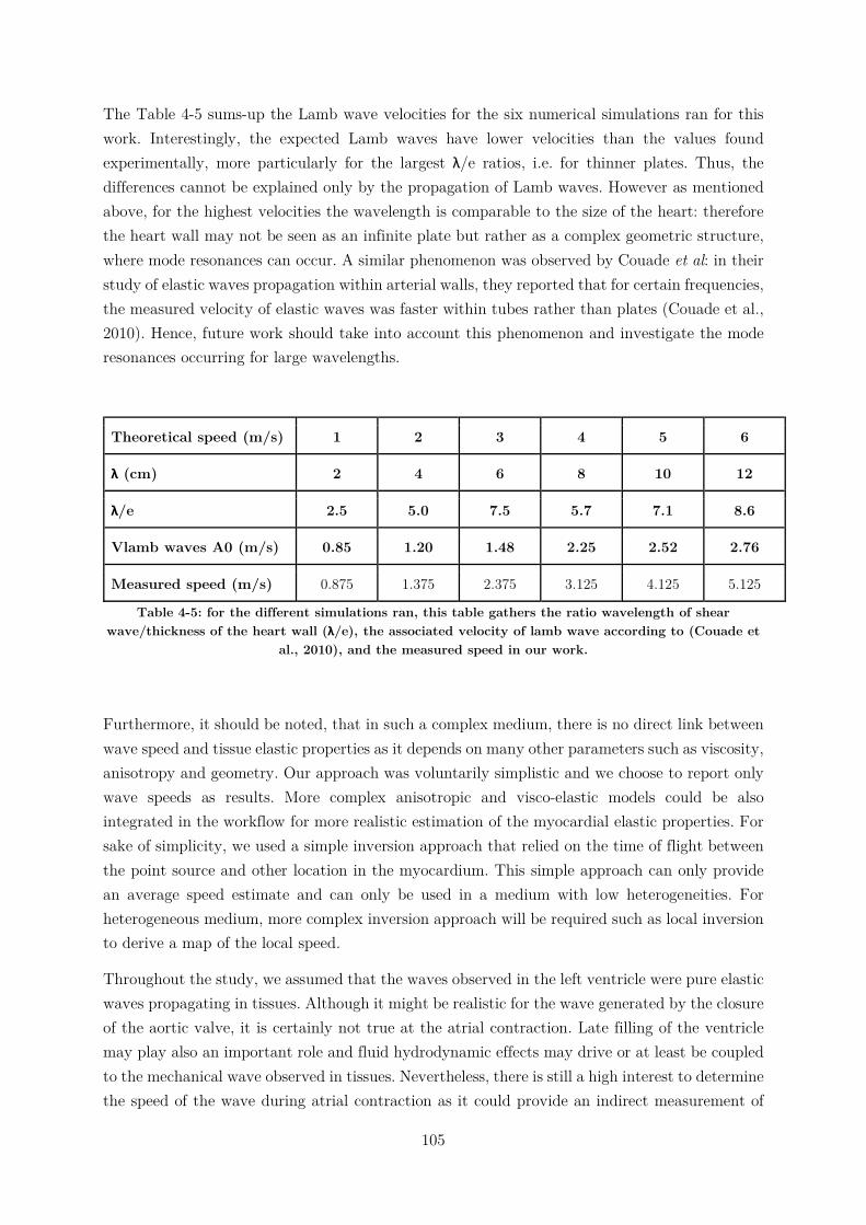
105

The Table 4-5 sums-up the Lamb wave velocities for the six numerical simulations ran for this work. Interestingly, the expected Lamb waves have lower velocities than the values found experimentally, more particularly for the largest λ/e ratios, i.e. for thinner plates. Thus, the differences cannot be explained only by the propagation of Lamb waves. However as mentioned above, for the highest velocities the wavelength is comparable to the size of the heart: therefore the heart wall may not be seen as an infinite plate but rather as a complex geometric structure, where mode resonances can occur. A similar phenomenon was observed by Couade et al: in their study of elastic waves propagation within arterial walls, they reported that for certain frequencies, the measured velocity of elastic waves was faster within tubes rather than plates (Couade et al., 2010). Hence, future work should take into account this phenomenon and investigate the mode resonances occurring for large wavelengths.

Theoretical speed (m/s) 1 2 3 4 5 6

λ (cm) 2 4 6 8 10 12

λ/e 2.5 5.0 7.5 5.7 7.1 8.6

Vlamb waves A0 (m/s) 0.85 1.20 1.48 2.25 2.52 2.76

Measured speed (m/s) 0.875 1.375 2.375 3.125 4.125 5.125

Table 4-5: for the different simulations ran, this table gathers the ratio wavelength of shear wave/thickness of the heart wall (λ/e), the associated velocity of lamb wave according to (Couade et

al., 2010), and the measured speed in our work.

Furthermore, it should be noted, that in such a complex medium, there is no direct link between wave speed and tissue elastic properties as it depends on many other parameters such as viscosity, anisotropy and geometry. Our approach was voluntarily simplistic and we choose to report only wave speeds as results. More complex anisotropic and visco-elastic models could be also integrated in the workflow for more realistic estimation of the myocardial elastic properties. For sake of simplicity, we used a simple inversion approach that relied on the time of flight between the point source and other location in the myocardium. This simple approach can only provide an average speed estimate and can only be used in a medium with low heterogeneities. For heterogeneous medium, more complex inversion approach will be required such as local inversion to derive a map of the local speed.

Throughout the study, we assumed that the waves observed in the left ventricle were pure elastic waves propagating in tissues. Although it might be realistic for the wave generated by the closure of the aortic valve, it is certainly not true at the atrial contraction. Late filling of the ventricle may play also an important role and fluid hydrodynamic effects may drive or at least be coupled to the mechanical wave observed in tissues. Nevertheless, there is still a high interest to determine the speed of the wave during atrial contraction as it could provide an indirect measurement of

106

the ventricular stiffness in diastole. This would be similar to the pulse wave velocity which is neither a pure elastic wave in the arterial wall nor a pure compressional wave propagating in the blood flow, but is still recognized as the best measurement of arterial stiffness.

We have shown the feasibility to derive in-vivo the wave velocity at two time of the cardiac cycle: at the end of systole after aortic valve closure, and at the end of diastole during atrial contraction. Both measurements could be of high interest for diagnostic purposes and may be used in different situations. On the one hand, ventricular stiffness plays a major role in diastolic dysfunction such as in patients with heart failure with preserved ejection fraction. The wave speed measured in diastole could be used as a global index of the ventricular passive stiffness. Currently, indexes of diastolic function measured by echocardiography remains indeed highly limited as they are not directly linked to the ventricular stiffness. The wave speed measured at the atrial contraction in this study was found in the same range than the mean shear velocity measured by shear wave elastography on the antero-septal wall on 60 volunteer using the remote generation of shear waves (Villemain et al., 2018b). This good agreement suggests that both techniques are measuring the same physical parameter. On the other hand, the assessment of elastic velocity at the aortic valve closure could be also of high interest, as systolic stiffness is known to be linked to the active contraction of the myocardium and has been shown correlated to myocardial contractility in isolated heart (Pernot et al., 2011). Therefore, this measurement could be a non-invasive index of ventricular contractility.

A limitation of this approach is that the elastic waves did not reach the entire left ventricle and the most apical part of the left ventricle could not be mapped. Another limitation of the method is the dependence with the source location. In some case, the source may be diffuse and difficult to identify precisely which may affect the robustness of the method. A third limitation was the manual segmentation of the left ventricle which was challenging due to the low contrast of the ultrafast images. An imaging sequence with a high contrast 3D image prior to the ultrafast acquisition could help a lot to provide a better manual or automatic segmentation. Moreover, our approach did not took into account the local anisotropy of the myocardium related to the fibres orientation, yet it has been proven that elastic waves propagate faster along the fibres than perpendicularly. Therefore, future developments should include this phenomenon, and comparison or merging with the work developed on 3DBTI should be of great interest.

4.5. Conclusion In this chapter, a framework to measure the velocity of naturally-induced elastic waves propagating in the left ventricle was developed. Firstly, numerical simulations were performed to evaluate the accuracy of our methodology and secondly, applications on elastic waves generated by the closing of the aortic valve and by the atrial kick were shown on two healthy volunteers. The elastic wave velocities of these events could be an interesting biomarker to detect and/or follow cardiac abnormalities in a clinical setup. Futures studies will focus on the complete evaluation of cardiac stiffness by the computation of the Young’s modulus of the myocardium, and the evaluation on larger cohorts of healthy and diseased hearts. Moreover, the link between

107

the anisotropy of the elastic wave speeds and the fibres orientation measured by BTI may be an interesting field of investigations.

108

4.6. Chapter Bibliography

Bercoff, J., Chaffai, S., Tanter, M., Sandrin, L., Catheline, S., Fink, M., Gennisson, J.L., Meunier, M., 2003. In vivo breast tumor detection using transient elastography. Ultrasound in Medicine & Biology 29, 1387–1396. https://doi.org/10.1016/S0301-5629(03)00978-5

Bercoff, J., Tanter, M., Chaffai, S., Fink, M., 2002. Ultrafast imaging of beamformed shear waves induced by the acoustic radiation force. Application to transient elastography, in: Proceedings of the 2002 IEEE Ultrasonics Symposium. pp. 1899–1902.

Berg, W.A., Cosgrove, D.O., Doré, C.J., Schäfer, F.K.W., Svensson, W.E., Hooley, R.J., Ohlinger, R., Mendelson, E.B., Balu-Maestro, C., Locatelli, M., Tourasse, C., Cavanaugh, B.C., Juhan, V., Stavros, A.T., Tardivon, A., Gay, J., Henry, J.-P., Cohen-Bacrie, C., For the BE1 Investigators, 2012. Shear-wave Elastography Improves the Specificity of Breast US: The BE1 Multinational Study of 939 Masses. Radiology 262, 435–449. https://doi.org/10.1148/radiol.11110640

Bonnet, B., Jourdan, F., du Cailar, G., Fesler, P., 2017. Noninvasive evaluation of left ventricular elastance according to pressure-volume curves modeling in arterial hypertension. American Journal of Physiology-Heart and Circulatory Physiology 313, H237–H243. https://doi.org/10.1152/ajpheart.00086.2017

Burkhoff, D., Mirsky, I., Suga, H., 2005. Assessment of systolic and diastolic ventricular properties via pressure-volume analysis: a guide for clinical, translational, and basic researchers. American Journal of Physiology-Heart and Circulatory Physiology 289, H501–H512. https://doi.org/10.1152/ajpheart.00138.2005

Catheline, S., 1998. INTERFEROMETRIE-SPECKLE ULTRASONORE : APPLICATION A LA MESURE D’ELASTICITE (Theses). Université Paris-Diderot - Paris VII.

Catheline, S., Souchon, R., Rupin, M., Brum, J., Dinh, A.H., Chapelon, J.-Y., 2013. Tomography iiiiiiiiiiiiifrom diffuse waves: Passive shear wave imaging using low frame rate scanners. Applied iiiiiiiiiiiiiPhysics Letters 103, 014101. https://doi.org/10.1063/1.4812515

Cohen, E., Cohen, L.D., Deffieux, T., Tanter, M., 2018. An Isotropic Minimal Path Based Framework for Segmentation and Quantification of Vascular Networks, in: Pelillo, M., Hancock, E. (Eds.), Energy Minimization Methods in Computer Vision and Pattern Recognition. Springer International Publishing, Cham, pp. 499–513. https://doi.org/10.1007/978-3-319-78199-0_33

Couade, M., Pernot, M., Prada, C., Messas, E., Emmerich, J., Bruneval, P., Criton, A., Fink, M., Tanter, M., 2010. Quantitative Assessment of Arterial Wall Biomechanical Properties Using Shear Wave Imaging. Ultrasound in Medicine & Biology 36, 1662–1676. https://doi.org/10.1016/j.ultrasmedbio.2010.07.004

109

Elgeti, T., Knebel, F., Hättasch, R., Hamm, B., Braun, J., Sack, I., 2014. Shear-wave Amplitudes Measured with Cardiac MR Elastography for Diagnosis of Diastolic Dysfunction. Radiology 271, 681–687. https://doi.org/10.1148/radiol.13131605

Elgeti, T., Tzschätzsch, H., Hirsch, S., Krefting, D., Klatt, D., Niendorf, T., Braun, J., Sack, I., 2012. Vibration-synchronized magnetic resonance imaging for the detection of myocardial elasticity changes. Magnetic Resonance in Medicine 67, 919–924. https://doi.org/10.1002/mrm.24185

Elliott, P., Andersson, B., Arbustini, E., Bilinska, Z., Cecchi, F., Charron, P., Dubourg, O., Kühl, U., Maisch, B., McKenna, W.J., Monserrat, L., Pankuweit, S., Rapezzi, C., Seferovic, P., Tavazzi, L., Keren, A., 2008. Classification of the cardiomyopathies: a position statement from the european society of cardiology working group on myocardial and pericardial diseases. Eur Heart J 29, 270–276. https://doi.org/10.1093/eurheartj/ehm342

Gallot, T., Catheline, S., Roux, P., Brum, J., Benech, N., Negreira, C., 2011. Passive iiiiiiiiiiiiielastography: shear-wave tomography from physiological-noise correlation in soft tissues. iiiiiiiiiiiiiIEEE Transactions on Ultrasonics, Ferroelectrics and Frequency Control 58, 1122–1126. iiiiiiiiiiiiihttps://doi.org/10.1109/TUFFC.2011.1920

Hoskins, A.C., Jacques, A., Bardswell, S.C., McKenna, W.J., Tsang, V., dos Remedios, C.G., Ehler, E., Adams, K., Jalilzadeh, S., Avkiran, M., Watkins, H., Redwood, C., Marston, S.B., Kentish, J.C., 2010. Normal passive viscoelasticity but abnormal myofibrillar force generation in human hypertrophic cardiomyopathy. Journal of Molecular and Cellular Cardiology 49, 737–745. https://doi.org/10.1016/j.yjmcc.2010.06.006

Kanai, H., 2005. Propagation of spontaneously actuated pulsive vibration in human heart wall and in vivo viscoelasticity estimation. IEEE transactions on ultrasonics, ferroelectrics, and frequency control 52, 1931–1942.

Kushwaha, S.S., Fallon, J.T., Fuster, V., 1997. Restrictive Cardiomyopathy. New England Journal of Medicine 336, 267–276. https://doi.org/10.1056/NEJM199701233360407

Nightingale, K.R., Palmeri, M.L., Nightingale, R.W., Trahey, G.E., 2001. On the feasibility of remote palpation using acoustic radiation force. The Journal of the Acoustical Society of America 110, 625–634. https://doi.org/10.1121/1.1378344

Papadacci, C., Pernot, M., Couade, M., Fink, M., Tanter, M., 2014. High Contrast Ultrafast Imaging of the Human Heart 29.

Pernot, M., Couade, M., Mateo, P., Crozatier, B., Fischmeister, R., Tanter, M., 2011. Real-Time Assessment of Myocardial Contractility Using Shear Wave Imaging. Journal of the American College of Cardiology 58, 65–72. https://doi.org/10.1016/j.jacc.2011.02.042


110

Pernot, M., Lee, W.-N., Bel, A., Mateo, P., Couade, M., Tanter, M., Crozatier, B., Messas, E., 2016. Shear Wave Imaging of Passive Diastolic Myocardial Stiffness. JACC: Cardiovascular Imaging 9, 1023–1030. https://doi.org/10.1016/j.jcmg.2016.01.022

Pislaru, C., 2004. Ultrasound Strain Imaging of Altered Myocardial Stiffness: Stunned Versus Infarcted Reperfused Myocardium. Circulation 109, 2905–2910. https://doi.org/10.1161/01.CIR.0000129311.73402.EF


Robert, B., Sinkus, R., Gennisson, J.-L., Fink, M., 2009. Application of DENSE-MR-elastography to the human heart. Magnetic Resonance in Medicine 62, 1155–1163. https://doi.org/10.1002/mrm.22124

Sabra, K.G., Conti, S., Roux, P., Kuperman, W.A., 2007. Passive in vivo elastography from iiiiiiiiiiiiiskeletal muscle noise. Applied Physics Letters 90, 194101. iiiiiiiiiiiiihttps://doi.org/10.1063/1.2737358


Sarvazyan, A.P., Rudenko, O.V., Swanson, S.D., Fowlkes, J.B., Emelianov, S.Y., 1998. Shear wave elasticity imaging: a new ultrasonic technology of medical diagnostics. Ultrasound in Medicine & Biology 24, 1419–1435. https://doi.org/10.1016/S0301-5629(98)00110-0

Sebag, F., Vaillant-Lombard, J., Berbis, J., Griset, V., Henry, J.F., Petit, P., Oliver, C., 2010. Shear Wave Elastography: A New Ultrasound Imaging Mode for the Differential Diagnosis of Benign and Malignant Thyroid Nodules. The Journal of Clinical Endocrinology & Metabolism 95, 5281–5288. https://doi.org/10.1210/jc.2010-0766

Sethian, J.A., 1999. Level Set Methods and Fast Marching Methods: Evolving Interfaces in Computational Geometry, Fluid Mechanics, Computer Vision, and Materials Science. Cambridge University Press.

Song, P., Bi, X., Mellema, D.C., Manduca, A., Urban, M.W., Greenleaf, J.F., Chen, S., 2016. Quantitative Assessment of Left Ventricular Diastolic Stiffness Using Cardiac Shear Wave Elastography: A Pilot Study. Journal of Ultrasound in Medicine 35, 1419–1427. https://doi.org/10.7863/ultra.15.08053

Song, P., Zhao, H., Urban, M.W., Manduca, A., Pislaru, S.V., Kinnick, R.R., Pislaru, C., Greenleaf, J.F., Chen, S., 2013. Improved Shear Wave Motion Detection Using Pulse-Inversion Harmonic Imaging With a Phased Array Transducer. IEEE Transactions on Medical Imaging 32, 2299–2310. https://doi.org/10.1109/TMI.2013.2280903

111

Treeby, B.E., Jaros, J., Rohrbach, D., Cox, B.T., 2014. Modelling elastic wave propagation using the k-Wave MATLAB Toolbox. IEEE, pp. 146–149. https://doi.org/10.1109/ULTSYM.2014.0037

van den Broek, J.H.J.M., van den Broek, M.H.L.M., 1980. Application of an ellipsoidal heart model in studying left ventricular contractions. Journal of Biomechanics 13, 493–503. https://doi.org/10.1016/0021-9290(80)90342-5

Varghese, T., 2009. Quasi-Static Ultrasound Elastography. Ultrasound Clin 4, 323–338. https://doi.org/10.1016/j.cult.2009.10.009

Villemain, O., Correia, M., Khraiche, D., Podetti, I., Meot, M., Legendre, A., Tanter, M., Bonnet, D., Pernot, M., 2018a. Myocardial Stiffness Assessment Using Shear Wave Imaging in Pediatric Hypertrophic Cardiomyopathy. JACC: Cardiovascular Imaging 11, 779–781. https://doi.org/10.1016/j.jcmg.2017.08.018

Villemain, O., Correia, M., Mousseaux, E., Baranger, J., Zarka, S., Podetti, I., Soulat, G., Damy, T., Hagège, A., Tanter, M., Pernot, M., Messas, E., 2018b. Myocardial Stiffness Evaluation Using Noninvasive Shear Wave Imaging in Healthy and Hypertrophic Cardiomyopathic Adults. JACC: Cardiovascular Imaging. https://doi.org/10.1016/j.jcmg.2018.02.002

Vos, H.J., van Dalen, B.M., Heinonen, I., Bosch, J.G., Sorop, O., Duncker, D.J., van der Steen, A.F.W., de Jong, N., 2017. Cardiac Shear Wave Velocity Detection in the Porcine Heart. Ultrasound in Medicine & Biology 43, 753–764. https://doi.org/10.1016/j.ultrasmedbio.2016.11.015

Wassenaar, P.A., Eleswarpu, C.N., Schroeder, S.A., Mo, X., Raterman, B.D., White, R.D., Kolipaka, A., 2016. Measuring age-dependent myocardial stiffness across the cardiac cycle using MR elastography: A reproducibility study: Myocardial Stiffness across the Cardiac Cycle. Magnetic Resonance in Medicine 75, 1586–1593. https://doi.org/10.1002/mrm.25760

Zile, M.R., Baicu, C.F., Gaasch, W.H., 2004. Diastolic Heart Failure — Abnormalities in Active Relaxation and Passive Stiffness of the Left Ventricle. New England Journal of Medicine 350, 1953–1959. https://doi.org/10.1056/NEJMoa032566

113

: 3D Ultrafast Imaging of

Myocardial Contraction Activation

5. : 3D Ultrafast Imaging of Myocardial Contraction Activation ......................................... 113

5.1. Introduction ............................................................................................................... 114

5.2. State of the art, motivation, objectives ..................................................................... 114

5.2.1. Electrophysiology of the heart and electrocardiogram ....................................... 114

5.2.2. Imaging the cardiac electrophysiology ................................................................ 115

5.2.3. Imaging the cardiac contraction ......................................................................... 116

5.2.4. Objectives ........................................................................................................... 117

5.3. 3D mapping ............................................................................................................... 118


5.3.2. Results ............................................................................................................... 120

5.3.2.1. Sinus rhythm .............................................................................................. 120

5.3.2.2. Pacing ......................................................................................................... 126

5.3.2.3. Effect of hypothermia ................................................................................. 127

5.3.3. Discussion ........................................................................................................... 129

5.4. Toward clinical applications ...................................................................................... 129


5.4.1.1. Adult acquisitions ....................................................................................... 130

5.4.1.2. Fetal acquisitions ........................................................................................ 131

5.4.1.3. Post-processing ........................................................................................... 131

5.4.2. Results ............................................................................................................... 132

5.4.2.1. Adults ......................................................................................................... 132

5.4.2.2. Fetus ........................................................................................................... 136

5.4.3. Discussion ........................................................................................................... 138

5.5. Conclusion ................................................................................................................. 141


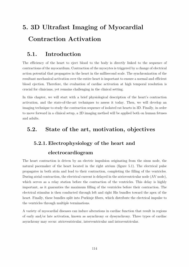
114

3D Ultrafast Imaging of Myocardial

Contraction Activation

5.1. Introduction The efficiency of the heart to eject blood to the body is directly linked to the sequence of contractions of the myocardium. Contraction of the myocytes is triggered by a change of electrical action potential that propagates in the heart in the millisecond scale. The synchronization of the resultant mechanical activation over the entire heart is important to ensure a normal and efficient blood ejection. Therefore, the evaluation of cardiac activation at high temporal resolution is crucial for clinicians, yet remains challenging in the clinical setting.

In this chapter, we will start with a brief physiological description of the heart’s contraction activation, and the state-of-the-art techniques to assess it today. Then, we will develop an imaging technique to study the contraction sequence of isolated rat hearts in 3D. Finally, in order to move forward in a clinical setup, a 2D imaging method will be applied both on human fetuses and adults.

5.2. State of the art, motivation, objectives

5.2.1. Electrophysiology of the heart and

electrocardiogram The heart contraction is driven by an electric impulsion originating from the sinus node, the natural pacemaker of the heart located in the right atrium (figure 5.1). The electrical pulse propagates in both atria and lead to their contraction, completing the filling of the ventricles. During atrial contraction, the electrical current is delayed in the atrioventricular node (AV node), which serves as a relay station before the contraction of the ventricles. This delay is highly important, as it guaranties the maximum filling of the ventricles before their contraction. The electrical stimulus is then conducted through left and right His bundles toward the apex of the heart. Finally, these bundles split into Purkinje fibers, which distribute the electrical impulse to the ventricles through multiple terminations.

A variety of myocardial diseases can induce alterations in cardiac function that result in regions of early and/or late activation, known as asynchrony or dyssynchrony. Three types of cardiac asynchrony may occur: atrioventricular, interventricular and intraventricular.

115

Figure 5.1 Activation sequence of the myocardium and contribution to ECG (Malmivuo and Plonsey, 1995).

The most widely used technique to analyze the electrical activation sequence of the heart is the electrocardiogram (ECG). It consists of a set of electrodes placed on the skin, recording the electrical field generated from the heart. ECG gives a global estimation of the heart electrical activity. Three main electrical events are visible on an ECG: the P wave, the QRS complex and the T wave, corresponding to the atrial contraction, ventricular contraction, and ventricular repolarization, respectively (figure 5.1). Numerous diagnoses can be suggested based on the analysis of the shape of the ECG, making it a tool of choice for clinicians. However, it has intrinsic limitations: it provides only electrical conduction information, and does not permit to localize precisely the origin of electrical signals measured. Therefore for an accurate diagnosis, conventional echocardiography is systematically used along ECG.

5.2.2. Imaging the cardiac electrophysiology

a) Electrocardiogram Imaging (ECGI)

In order to obtain a map of electrical activity of the myocardium, an ECG is performed with a large number of electrodes placed over the whole torso of patients. By coupling electrical measurements to CT or MRI scans, it is possible to solve the inverse-problem of the electrical propagation from the heart to the torso, and compute an electrical activation map (Ramanathan et al., 2004; Zhang et al., 2005; Ramanathan, 2006). However, this technology is costly and not yet spread into routine clinics (Nash and Pullan, 2005), and requires a prior CT or a MRI scan. Moreover, it allows only the reconstruction of the epicardial potential.

b) Catheterization

The most widely used solution to image the cardiac electrophysiology in the clinical setting is the insertion of a catheter containing an array of electrodes within the heart. The electrodes in



116

contact with the myocardium measure action potentials, a brief change of voltage that triggers the muscle contraction. Such electrophysiology studies allow to investigate the cause and location of various conduction problems, and treat them within a single procedure. Limitations of this technique are induced by the cardiac catheterization: it is time consuming, costly, highly invasive, and complications may occur during the procedure. Moreover, it allows the measurement of endocardial potentials only. Such a catheter can also be used to perform ablation of abnormal electrical pathways.

c) Optical mapping

Optical imaging techniques have been used to monitor cardiac action potentials since the mid-70s. A voltage-sensitive dye binds to the myocardium and is illuminated by specific monochromatic light; when the cell undergoes electrical activation, the dye fluoresce. The emitted fluorescence is recorded by a camera (Rosenbaum et al., 1992; Salama and Morad, 1976). Voltage sensitive mapping can be used to image the propagation of electrical activation of various species including rat, mice, rabbit, pigs (Marian et al., 1999; Nygren et al., 2000, 2003; Matiukas et al., 2007) and offers a high spatial resolution. However, because motion of the heart would create artefacts, it is required to inhibit the mechanical contraction of the myocardium using drugs. Moreover, as of today, optical mapping is performed on isolated, perfused hearts, and is not usable in-vivo (Herron et al., 2012).

5.2.3. Imaging the cardiac contraction

a. Echocardiography for the clinical evaluation of cardiac dyssynchrony

Conventional echography provides a wide variety of modes allowing for the evaluation of cardiac synchronization. In particular, the evaluation of the left ventricle activation sequence is an active research field, as abnormalities of regional LV contraction are the principal factor associated with contractile impairment (Gorcsan et al., 2008). In the following paragraphs, we will therefore briefly review the existing techniques to assess it.

The simplest way of measuring the left ventricle activation delay is to perform an M-Mode in the parasternal long-axis or short axis view: this provide a simple and effective evaluation of the delay between the movement of the lateral walls and septum to eject blood out of the ventricle.

Tissue Doppler imaging allows for the evaluation of cardiac function through the radial movements (parasternal long and short axis views) and longitudinal movement (4-chambers, 3-chambers and 2-chambers apical views). Both color tissue Doppler or pulsed tissue Doppler can be used to measure and compare the time of peak velocity of a few segments of the LV wall to assess if a resynchronization is needed (Notabartolo et al., 2004). Strain and strain rate imaging have the advantage of being able to differentiate active deformations from passive movements and thus can be used to identify asynchrony. Tissue Doppler-derived strain and strain rate imaging were introduced several years ago (D’hooge, 2000) and can be used to evaluate the activation sequence (Gorcsan et al., 2008). Moreover, strain and strain rates can also be

117

calculated using speckle-tracking algorithms, with the advantages of removing the Doppler-induced limitations (sensitivity to noise, measurements of velocities along the probe axis only, inter-operator variability), and allows for full 2D or 3D analysis of cardiac contraction synchronization (Delgado et al., 2008; Geyer et al., 2010; Suffoletto, 2006). Limitations of speckle-tracking are the need of good quality greyscale images which limits the temporal resolution, and the high computational cost of 3D calculations.

b. Ultrafast imaging

Ultrafast imaging offers the possibility to image the heart with a large field of view and a high frame rate which is particularly interesting to observe the dynamics of very rapid mechanical events such as the activation of the myocardial contraction. Following the electrical activation of the myocytes, the transient mechanical deformation of the myocardium can be observed at the millisecond scale. The mechanical activation sequence was shown to be linearly correlated to the electrical activation using MRI (Wyman et al., 1999; Faris et al., 2003) and ultrafast echocardiography (Konofagou and Provost, 2012). Electromechanical Wave Imaging (EWI) was introduced as a noninvasive, ultrasound-based imaging modality to map the electromechanical wave. EWI relies the calculation of axial displacements (Pernot and Konofagou, 2005; Pernot et al., 2007) or strains (Provost et al., 2010) and was used to characterize electromechanical waves in various studies including mice (Konofagou et al., 2010), normal and ischemic canines (Pernot and Konofagou, 2005; Provost et al., 2010), and humans (Konofagou and Provost, 2012). Since the electromechanical wave propagation in a beating heart is a complex 3D phenomenon, Provost et al. introduced the combination of multiple 2D standard echocardiographic views (four-chambers, two-chamber) to a generate 3D mapping (Provost et al., 2011). Later, an algorithm allowing for the interpolation of a full 3D volume has been proposed (Nauleau et al., 2017). However, these 3D renderings require multiple 2D acquisitions over several heart beats and their synthetic recombination a posteriori which is challenging to perform in clinical practice.

5.2.4. Objectives The objectives of this work is to develop an imaging tool that can map the sequence of cardiac mechanical activation using 3D ultrafast imaging, which would allow for the full analysis of cardiac activation sequence within a single heartbeat. As cardiac mechanics are complex in-vivo, we used a simple model of isolated heart to assess the feasibility of the technique. Such a model presents many advantages for this study because the physiological parameters are accurately controlled and the number of undesired mechanical events is reduced compared to in-vivo conditions. The objectives of this work were: 1) to develop 3D ultrafast imaging of the cardiac mechanical activation of isolated rat hearts 2) to validate the methods against electrophysiological measurements and 3) to investigate the feasibility on human patients. The chapter is divided into two parts: firstly, we will perform 4D ultrafast ultrasound scanner to map in 3D the contraction activation sequence of isolated rat heats. Secondly, we will develop a method to move the technique towards the clinical setting, using a standard 2D ultrafast ultrasound scanner. Applications on adults’ and fetus’ hearts will be shown.

118

5.3. 3D mapping The objective of this part is to develop a method to image in 3D the myocardial contraction activation of isolated rat hearts within a single heartbeat. Isolated and perfused hearts present the advantage of being a simplified model to study. Parameters such as pressure, volume, temperature, coronary flow rates, heart beat etc. are well controlled and adjustable by the operator. For our study, the isolated heart presents also advantages on the mechanical point of view with a reduced number of mechanical events. As the perfusion is retrograde (from the aorta), the aortic valve is always closed and there is no flow at all in the ventricular and atrial cavities. As valve closure and opening can be a strong source of mechanical activity in-vivo, the isolated heart model is a good model to remove all these effects.

Firstly, the acquisition and analysis of contraction activation will be investigated in sinus rhythm and under pacing condition. The mechanical activation sequence will be quantified for different physiological conditions. Finally, the mechanical activation timing will be compared with electrophysiological measurements.


a) Isolated heart model, or Langendorff model (figure 5.2)

The isolated heart model used in this work was developed by Oscar Langendorff in the late 19th century (Langendorff, 1895) and is still widely used today in a variety of applications (Skrzypiec-Spring et al., 2007). The methodology described originally has not changed drastically over the years: the heart is perfused retrogradely by the aorta, thus forcing the aortic valve to close. The perfusate is entering the coronary vasculature via the aortic root and is eventually drained in the right atrium. Therefore, it can exit the heart without entering into the ventricles, which both remain mainly dry. In addition, a balloon is inserted into the left ventricle through the mitral valve. The balloon needs to be as compliant as possible to not interfere with the movements of the left ventricle, and is mounted on a tube and filled with fluid that allows for the adjusting of the pressure and volume of the balloon, allowing for the control of the contractility of the left ventricle according to Frank-Staring curves.

The Langendorff setup is extremely helpful to study the heart’s physiology. In our case, it will guaranties the best ultrasound acquisitions quality, as there won’t be any surrounding tissues and rib cage creating possible artefacts. Moreover, as discussed previously, the cardiac valves are not opening nor closing: this will greatly ease the visualization of cardiac mechanical activation, as there won’t be undesired elastic waves created by the closure of the atrioventricular valves. Furthermore, this setup is helping to validate the findings of ultrasound. Indeed, the isolation of the heart allows to put electrodes at any location of the epicardium: either to measure local electrical activation, or to pace the heart and compare the position of the electrical stimulation and the earliest mechanical activation points found after post-processing. Finally, the

119

temperature of the perfusate being precisely controlled, it gives a straightforward opportunity to study the effect of hypothermia on the heart.

b) Experimental setup

In our study, rat hearts were perfused by a Krebs-Henseleit solution and immerged in a latex balloon transparent to ultrasound, filled with the excess of perfusate (see figure 5.2). Electrophysiological electrodes were placed in contact with the right and left ventricles epicardium, and a pacing electrode was freely placed on the heart. The temperature was varied from 27°C to 37°C to study the effect of hypothermia on the activation sequence.

A 2D matrix array (8MHz, 32x32 elements, 0.3mm pitch) driven by a customized, programmable, 1024-channel ultrasound scanner was used to perform 600-ms-long 2D plane-wave acquisitions at 3000 volumes/s in the apical view. Electric signals of all electrodes were recorded during acquisitions. The pacing signal was a 10ms-pulse, which frequency and voltage were in the ranges [250-300] beats-per-minutes and [0.1-2]V, respectively, to ensure effectiveness of pacing. Acquisitions were repeated over 5 rats (average weight 228g±23g) with various temperatures within the range 26°C-37°C and various pacing locations.

Figure 5.2 Sketch of Langendorff setup, showing the inflatable balloon in the left ventricle, the perfusion, the electrophysiological and pacing electrodes. The position of all electrodes can be

rearranged during the experiments. Sketch adapted from (Dick, 1998).

c) Post processing

IQ beamforming allowed for the segmentation of the myocardium based on B-Mode intensity. Inter-volumes axial displacements and accelerations were mapped in the myocardium using the Kasai algorithm (Kasai et al., 1985) and a smooth derivative filter (Luo et al., 2004), respectively.

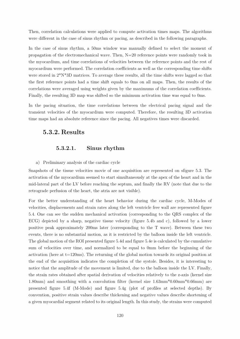
120

Then, correlation calculations were applied to compute activation times maps. The algorithms were different in the case of sinus rhythm or pacing, as described in the following paragraphs.

In the case of sinus rhythm, a 50ms window was manually defined to select the moment of propagation of the electromechanical wave. Then, N=20 reference points were randomly took in the myocardium, and time correlations of velocities between the reference points and the rest of myocardium were performed. The correlation coefficients as well as the corresponding time shifts were stored in 2*N*3D matrices. To average these results, all the time shifts were lagged so that the first reference points had a time shift equals to 0ms on all maps. Then, the results of the correlations were averaged using weights given by the maximums of the correlation coefficients. Finally, the resulting 3D map was shifted so the minimum activation time was equal to 0ms.

In the pacing situation, the time correlations between the electrical pacing signal and the transient velocities of the myocardium were computed. Therefore, the resulting 3D activation time maps had an absolute reference since the pacing. All negatives times were discarded.

5.3.2. Results

5.3.2.1. Sinus rhythm

a) Preliminary analysis of the cardiac cycle

Snapshots of the tissue velocities movie of one acquisition are represented on sfigure 5.3. The activation of the myocardium seemed to start simultaneously at the apex of the heart and in the mid-lateral part of the LV before reaching the septum, and finally the RV (note that due to the retrograde perfusion of the heart, the atria are not visible).

For the better understanding of the heart behavior during the cardiac cycle, M-Modes of velocities, displacements and strain rates along the left ventricle free wall are represented figure 5.4. One can see the sudden mechanical activation (corresponding to the QRS complex of the ECG) depicted by a sharp, negative tissue velocity (figure 5.4b and c), followed by a lower positive peak approximately 200ms later (corresponding to the T wave). Between these two events, there is no substantial motion, as it is restricted by the balloon inside the left ventricle. The global motion of the ROI presented figure 5.4d and figure 5.4e is calculated by the cumulative sum of velocities over time, and normalized to be equal to 0mm before the beginning of the activation (here at t=120ms). The returning of the global motion towards its original position at the end of the acquisition indicates the completion of the systole. Besides, it is interesting to notice that the amplitude of the movement is limited, due to the balloon inside the LV. Finally, the strain rates obtained after spatial derivation of velocities relatively to the z-axis (kernel size 1.80mm) and smoothing with a convolution filter (kernel size 1.63mm*0.60mm*0.66mm) are presented figure 5.4f (M-Mode) and figure 5.4g (plot of profiles at selected depths). By convention, positive strain values describe thickening and negative values describe shortening of a given myocardial segment related to its original length. In this study, the strains were computed

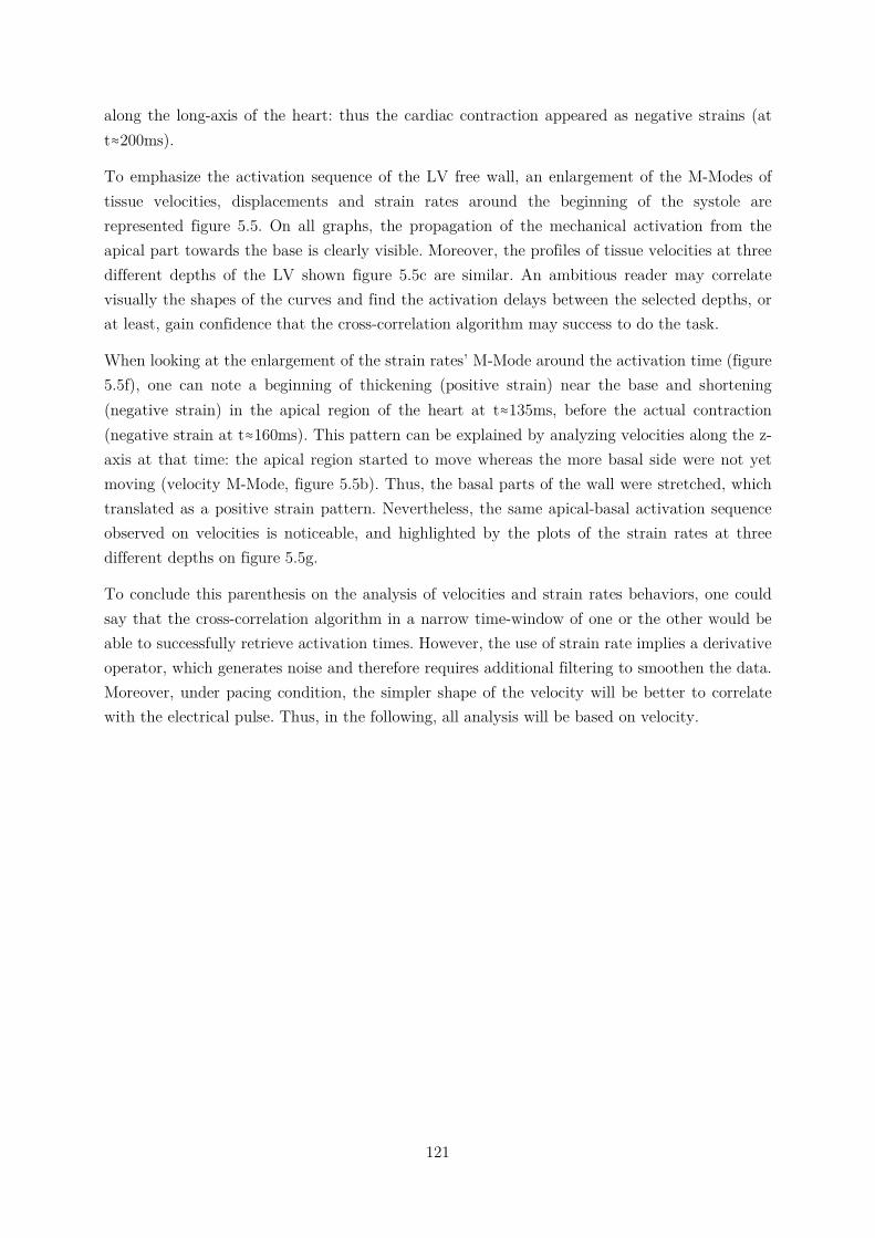
121

along the long-axis of the heart: thus the cardiac contraction appeared as negative strains (at t≈200ms).

To emphasize the activation sequence of the LV free wall, an enlargement of the M-Modes of tissue velocities, displacements and strain rates around the beginning of the systole are represented figure 5.5. On all graphs, the propagation of the mechanical activation from the apical part towards the base is clearly visible. Moreover, the profiles of tissue velocities at three different depths of the LV shown figure 5.5c are similar. An ambitious reader may correlate visually the shapes of the curves and find the activation delays between the selected depths, or at least, gain confidence that the cross-correlation algorithm may success to do the task.

When looking at the enlargement of the strain rates’ M-Mode around the activation time (figure 5.5f), one can note a beginning of thickening (positive strain) near the base and shortening (negative strain) in the apical region of the heart at t≈135ms, before the actual contraction (negative strain at t≈160ms). This pattern can be explained by analyzing velocities along the z-axis at that time: the apical region started to move whereas the more basal side were not yet moving (velocity M-Mode, figure 5.5b). Thus, the basal parts of the wall were stretched, which translated as a positive strain pattern. Nevertheless, the same apical-basal activation sequence observed on velocities is noticeable, and highlighted by the plots of the strain rates at three different depths on figure 5.5g.

To conclude this parenthesis on the analysis of velocities and strain rates behaviors, one could say that the cross-correlation algorithm in a narrow time-window of one or the other would be able to successfully retrieve activation times. However, the use of strain rate implies a derivative operator, which generates noise and therefore requires additional filtering to smoothen the data. Moreover, under pacing condition, the simpler shape of the velocity will be better to correlate with the electrical pulse. Thus, in the following, all analysis will be based on velocity.

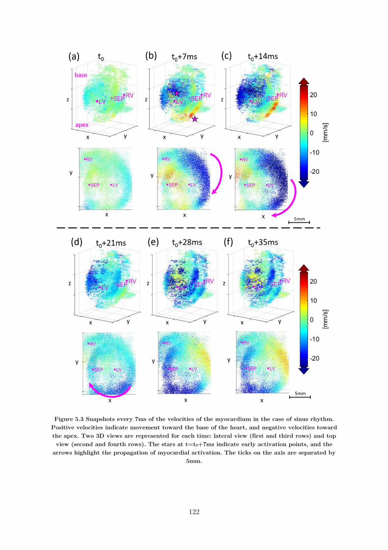
122

Figure 5.3 Snapshots every 7ms of the velocities of the myocardium in the case of sinus rhythm. Positive velocities indicate movement toward the base of the heart, and negative velocities toward the apex. Two 3D views are represented for each time: lateral view (first and third rows) and top view (second and fourth rows). The stars at t=t0+7ms indicate early activation points, and the

arrows highlight the propagation of myocardial activation. The ticks on the axis are separated by 5mm.

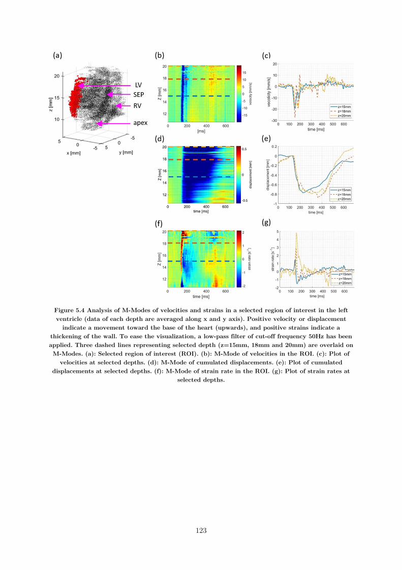
123

Figure 5.4 Analysis of M-Modes of velocities and strains in a selected region of interest in the left ventricle (data of each depth are averaged along x and y axis). Positive velocity or displacement

indicate a movement toward the base of the heart (upwards), and positive strains indicate a thickening of the wall. To ease the visualization, a low-pass filter of cut-off frequency 50Hz has been applied. Three dashed lines representing selected depth (z=15mm, 18mm and 20mm) are overlaid on M-Modes. (a): Selected region of interest (ROI). (b): M-Mode of velocities in the ROI. (c): Plot of

velocities at selected depths. (d): M-Mode of cumulated displacements. (e): Plot of cumulated displacements at selected depths. (f): M-Mode of strain rate in the ROI. (g): Plot of strain rates at

selected depths.

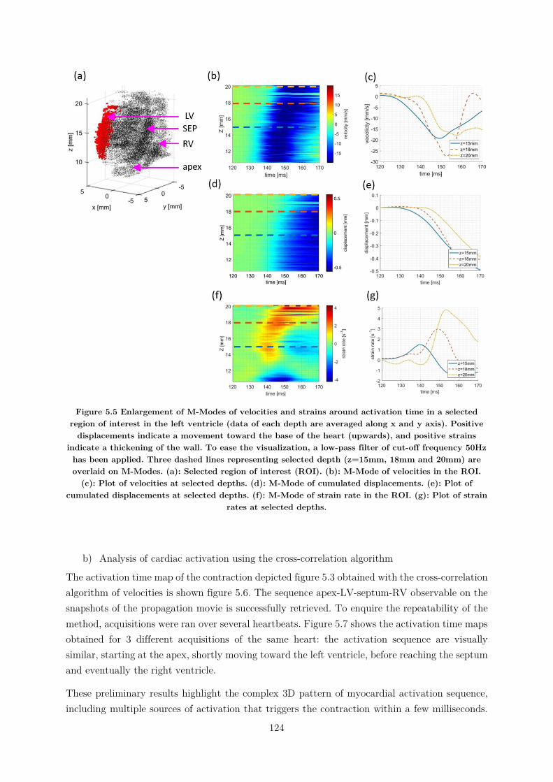
124

Figure 5.5 Enlargement of M-Modes of velocities and strains around activation time in a selected region of interest in the left ventricle (data of each depth are averaged along x and y axis). Positive

displacements indicate a movement toward the base of the heart (upwards), and positive strains indicate a thickening of the wall. To ease the visualization, a low-pass filter of cut-off frequency 50Hz has been applied. Three dashed lines representing selected depth (z=15mm, 18mm and 20mm) are overlaid on M-Modes. (a): Selected region of interest (ROI). (b): M-Mode of velocities in the ROI.

(c): Plot of velocities at selected depths. (d): M-Mode of cumulated displacements. (e): Plot of cumulated displacements at selected depths. (f): M-Mode of strain rate in the ROI. (g): Plot of strain

rates at selected depths.

b) Analysis of cardiac activation using the cross-correlation algorithm

The activation time map of the contraction depicted figure 5.3 obtained with the cross-correlation algorithm of velocities is shown figure 5.6. The sequence apex-LV-septum-RV observable on the snapshots of the propagation movie is successfully retrieved. To enquire the repeatability of the method, acquisitions were ran over several heartbeats. Figure 5.7 shows the activation time maps obtained for 3 different acquisitions of the same heart: the activation sequence are visually similar, starting at the apex, shortly moving toward the left ventricle, before reaching the septum and eventually the right ventricle.

These preliminary results highlight the complex 3D pattern of myocardial activation sequence, including multiple sources of activation that triggers the contraction within a few milliseconds.

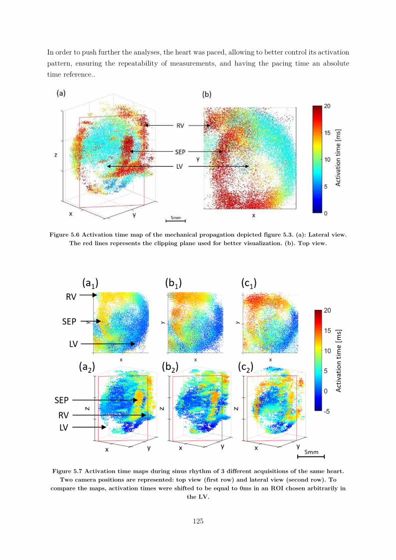
125

In order to push further the analyses, the heart was paced, allowing to better control its activation pattern, ensuring the repeatability of measurements, and having the pacing time an absolute time reference..

Figure 5.6 Activation time map of the mechanical propagation depicted figure 5.3. (a): Lateral view. The red lines represents the clipping plane used for better visualization. (b). Top view.

Figure 5.7 Activation time maps during sinus rhythm of 3 different acquisitions of the same heart. Two camera positions are represented: top view (first row) and lateral view (second row). To

compare the maps, activation times were shifted to be equal to 0ms in an ROI chosen arbitrarily in the LV.

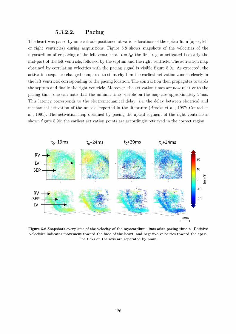
126

5.3.2.2. Pacing The heart was paced by an electrode positioned at various locations of the epicardium (apex, left or right ventricles) during acquisitions. Figure 5.8 shows snapshots of the velocities of the myocardium after pacing of the left ventricle at 𝑡 = 𝑡 : the first region activated is clearly the mid-part of the left ventricle, followed by the septum and the right ventricle. The activation map obtained by correlating velocities with the pacing signal is visible figure 5.9a. As expected, the activation sequence changed compared to sinus rhythm: the earliest activation zone is clearly in the left ventricle, corresponding to the pacing location. The contraction then propagates towards the septum and finally the right ventricle. Moreover, the activation times are now relative to the pacing time: one can note that the minima times visible on the map are approximately 25ms. This latency corresponds to the electromechanical delay, i.e. the delay between electrical and mechanical activation of the muscle, reported in the literature (Brooks et al., 1987; Conrad et al., 1991). The activation map obtained by pacing the apical segment of the right ventricle is shown figure 5.9b: the earliest activation points are accordingly retrieved in the correct region.

Figure 5.8 Snapshots every 5ms of the velocity of the myocardium 19ms after pacing time t0. Positive velocities indicates movement toward the base of the heart, and negative velocities toward the apex.

The ticks on the axis are separated by 5mm.

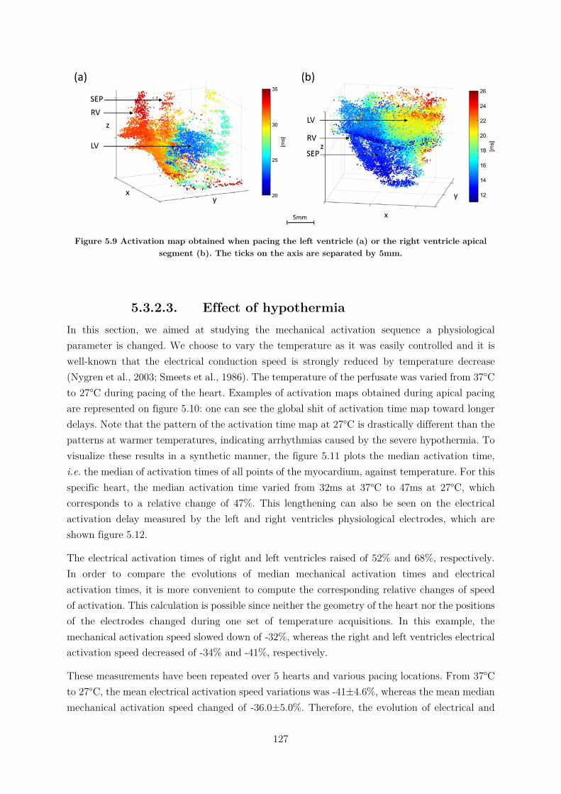
127

Figure 5.9 Activation map obtained when pacing the left ventricle (a) or the right ventricle apical segment (b). The ticks on the axis are separated by 5mm.

5.3.2.3. Effect of hypothermia In this section, we aimed at studying the mechanical activation sequence a physiological parameter is changed. We choose to vary the temperature as it was easily controlled and it is well-known that the electrical conduction speed is strongly reduced by temperature decrease (Nygren et al., 2003; Smeets et al., 1986). The temperature of the perfusate was varied from 37°C to 27°C during pacing of the heart. Examples of activation maps obtained during apical pacing are represented on figure 5.10: one can see the global shit of activation time map toward longer delays. Note that the pattern of the activation time map at 27°C is drastically different than the patterns at warmer temperatures, indicating arrhythmias caused by the severe hypothermia. To visualize these results in a synthetic manner, the figure 5.11 plots the median activation time, i.e. the median of activation times of all points of the myocardium, against temperature. For this specific heart, the median activation time varied from 32ms at 37°C to 47ms at 27°C, which corresponds to a relative change of 47%. This lengthening can also be seen on the electrical activation delay measured by the left and right ventricles physiological electrodes, which are shown figure 5.12.

The electrical activation times of right and left ventricles raised of 52% and 68%, respectively. In order to compare the evolutions of median mechanical activation times and electrical activation times, it is more convenient to compute the corresponding relative changes of speed of activation. This calculation is possible since neither the geometry of the heart nor the positions of the electrodes changed during one set of temperature acquisitions. In this example, the mechanical activation speed slowed down of -32%, whereas the right and left ventricles electrical activation speed decreased of -34% and -41%, respectively.

These measurements have been repeated over 5 hearts and various pacing locations. From 37°C to 27°C, the mean electrical activation speed variations was -41±4.6%, whereas the mean median mechanical activation speed changed of -36.0±5.0%. Therefore, the evolution of electrical and

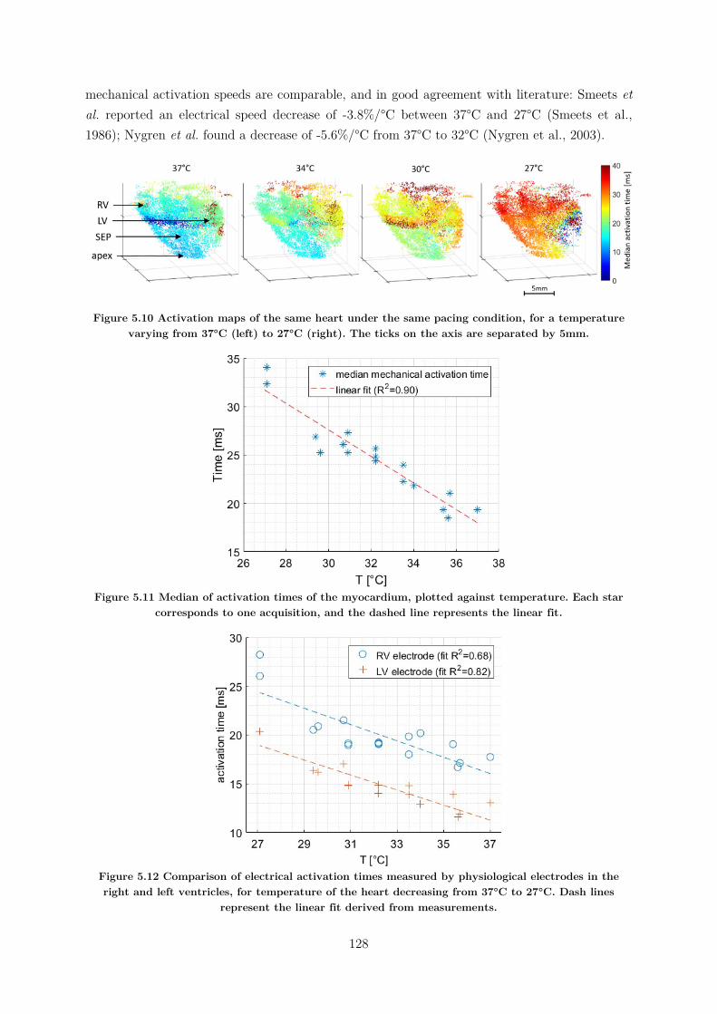
128

mechanical activation speeds are comparable, and in good agreement with literature: Smeets et al. reported an electrical speed decrease of -3.8%/°C between 37°C and 27°C (Smeets et al., 1986); Nygren et al. found a decrease of -5.6%/°C from 37°C to 32°C (Nygren et al., 2003).

Figure 5.10 Activation maps of the same heart under the same pacing condition, for a temperature varying from 37°C (left) to 27°C (right). The ticks on the axis are separated by 5mm.

Figure 5.11 Median of activation times of the myocardium, plotted against temperature. Each star

corresponds to one acquisition, and the dashed line represents the linear fit.

Figure 5.12 Comparison of electrical activation times measured by physiological electrodes in the right and left ventricles, for temperature of the heart decreasing from 37°C to 27°C. Dash lines

represent the linear fit derived from measurements.

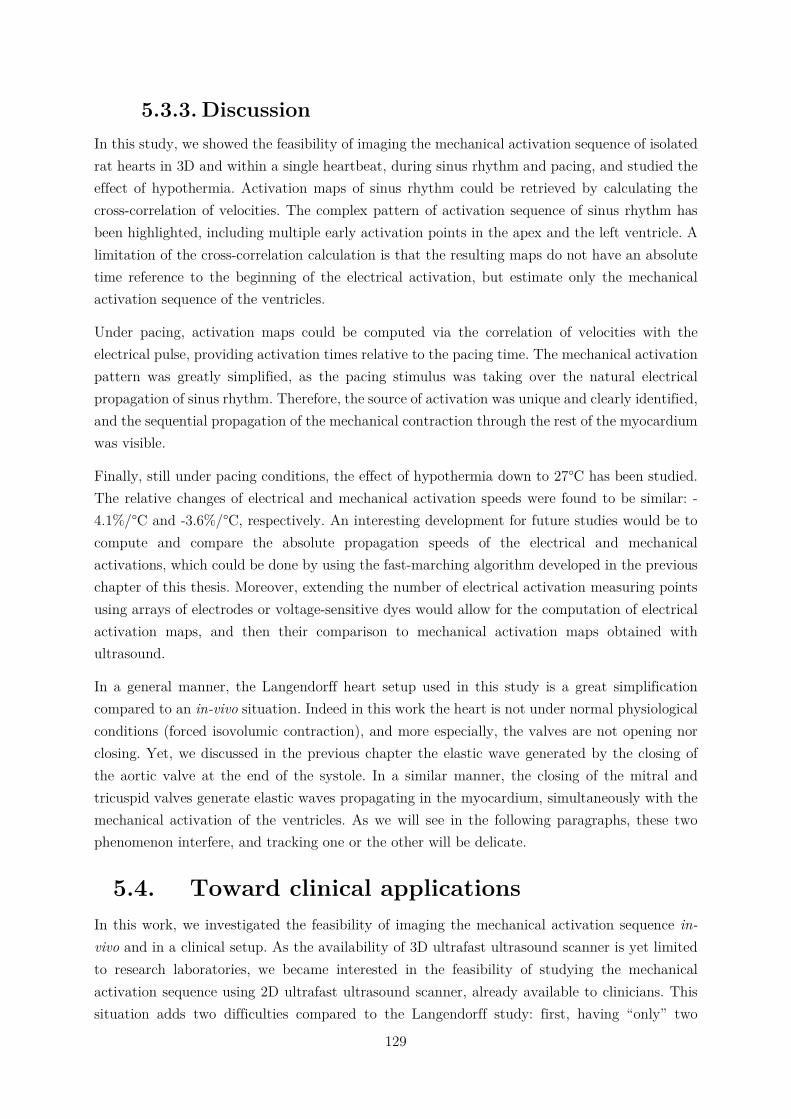
129

5.3.3. Discussion In this study, we showed the feasibility of imaging the mechanical activation sequence of isolated rat hearts in 3D and within a single heartbeat, during sinus rhythm and pacing, and studied the effect of hypothermia. Activation maps of sinus rhythm could be retrieved by calculating the cross-correlation of velocities. The complex pattern of activation sequence of sinus rhythm has been highlighted, including multiple early activation points in the apex and the left ventricle. A limitation of the cross-correlation calculation is that the resulting maps do not have an absolute time reference to the beginning of the electrical activation, but estimate only the mechanical activation sequence of the ventricles.

Under pacing, activation maps could be computed via the correlation of velocities with the electrical pulse, providing activation times relative to the pacing time. The mechanical activation pattern was greatly simplified, as the pacing stimulus was taking over the natural electrical propagation of sinus rhythm. Therefore, the source of activation was unique and clearly identified, and the sequential propagation of the mechanical contraction through the rest of the myocardium was visible.

Finally, still under pacing conditions, the effect of hypothermia down to 27°C has been studied. The relative changes of electrical and mechanical activation speeds were found to be similar: -4.1%/°C and -3.6%/°C, respectively. An interesting development for future studies would be to compute and compare the absolute propagation speeds of the electrical and mechanical activations, which could be done by using the fast-marching algorithm developed in the previous chapter of this thesis. Moreover, extending the number of electrical activation measuring points using arrays of electrodes or voltage-sensitive dyes would allow for the computation of electrical activation maps, and then their comparison to mechanical activation maps obtained with ultrasound.

In a general manner, the Langendorff heart setup used in this study is a great simplification compared to an in-vivo situation. Indeed in this work the heart is not under normal physiological conditions (forced isovolumic contraction), and more especially, the valves are not opening nor closing. Yet, we discussed in the previous chapter the elastic wave generated by the closing of the aortic valve at the end of the systole. In a similar manner, the closing of the mitral and tricuspid valves generate elastic waves propagating in the myocardium, simultaneously with the mechanical activation of the ventricles. As we will see in the following paragraphs, these two phenomenon interfere, and tracking one or the other will be delicate.

5.4. Toward clinical applications In this work, we investigated the feasibility of imaging the mechanical activation sequence in-vivo and in a clinical setup. As the availability of 3D ultrafast ultrasound scanner is yet limited to research laboratories, we became interested in the feasibility of studying the mechanical activation sequence using 2D ultrafast ultrasound scanner, already available to clinicians. This situation adds two difficulties compared to the Langendorff study: first, having “only” two

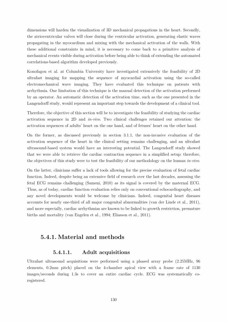
130

dimensions will harden the visualization of 3D mechanical propagations in the heart. Secondly, the atrioventricular valves will close during the ventricular activation, generating elastic waves propagating in the myocardium and mixing with the mechanical activation of the walls. With these additional constraints in mind, it is necessary to come back to a primitive analysis of mechanical events visible during activation before being able to think of extending the automated correlations-based algorithm developed previously.

Konofagou et al. at Columbia University have investigated extensively the feasibility of 2D ultrafast imaging for mapping the sequence of myocardial activation using the so-called electromechanical wave imaging. They have evaluated this technique on patients with arrhythmia. One limitation of this technique is the manual detection of the activation performed by an operator. An automatic detection of the activation time, such as the one presented in the Langendorff study, would represent an important step towards the development of a clinical tool.

Therefore, the objective of this section will be to investigate the feasibility of studying the cardiac activation sequence in 2D and in-vivo. Two clinical challenges retained our attention: the activation sequences of adults’ heart on the one hand, and of fetuses’ heart on the other hand.

On the former, as discussed previously in section 3.1.1, the non-invasive evaluation of the activation sequence of the heart in the clinical setting remains challenging, and an ultrafast ultrasound-based system would have an interesting potential. The Langendorff study showed that we were able to retrieve the cardiac contraction sequence in a simplified setup: therefore, the objectives of this study were to test the feasibility of our methodology on the human in-vivo.

On the latter, clinicians suffer a lack of tools allowing for the precise evaluation of fetal cardiac function. Indeed, despite being an extensive field of research over the last decades, assessing the fetal ECG remains challenging (Sameni, 2010) as its signal is covered by the maternal ECG. Thus, as of today, cardiac function evaluation relies only on conventional echocardiography, and any novel developments would be welcome by clinicians. Indeed, congenital heart diseases accounts for nearly one-third of all major congenital abnormalities (van der Linde et al., 2011), and more especially, cardiac arrhythmias are known to be linked to growth restriction, premature births and mortality (van Engelen et al., 1994; Eliasson et al., 2011).


5.4.1.1. Adult acquisitions Ultrafast ultrasound acquisitions were performed using a phased array probe (2.25MHz, 96 elements, 0.2mm pitch) placed on the 4-chamber apical view with a frame rate of 1130 images/seconds during 1.3s to cover an entire cardiac cycle. ECG was systematically co-registered.

131

5.4.1.2. Fetal acquisitions Ultrafast ultrasound exams were performed aside routine follow-ups of 5 fetuses (18, 22, 22, 25, 32 weeks of pregnancy) using a linear probe (6MHz, 128 elements, 0.2mm pitch). 1250 frames of a 4-chamber view were acquired at a frame rate of 2532Hz.

Clinical data accessible were collected from conventional modes (B-Mode, Tissue Doppler, Pulsed Doppler, M-Mode): heart rate, E/A ration E’/A’ ratio, systolic duration, diastolic duration, PR interval.

5.4.1.3. Post-processing RF data were beamformed and demodulated to IQ signals. Axial velocities were estimated using the Kasai algorithm (Kasai et al., 1985), smoothed spatially by convolution filters (kernel sizes of 1.5° * 6.8mm before scan conversion in the case of the adults and 1.3mm*1.3mm for fetal acquisitions). Tissue accelerations were calculated by the time derivative over 14ms for the adults and 7.9ms for the fetuses.

To visualize mechanical events and their propagations in the hearts walls, curves were manually drawn over selected segments of the myocardium (i.e. right atrium free wall, atrial and ventricular septa, right and left ventricle free walls)4 using B-Mode images. M-Modes of tissue velocities and accelerations of points along those curves were then displayed.

The velocities M-Modes allowed to retrieve the different phases of the cardiac cycle during the acquisitions (and the comparison with the ECG that could be acquired on adults). To define the mechanical activation of the walls, we used the acceleration data rather than the velocity. Indeed, the activation is depicted by a sudden change of tissue velocity, i.e., a peak of acceleration. The correlation algorithm previously used for the Langendorff study is actually comparing the velocity profiles of each point of the myocardium, but to be done visually using M-Modes, it is more relevant to search for maxima of accelerations. Furthermore, it is important to keep in mind the direction of motion of each wall during the mechanical contraction, as this information will be used to identify the corresponding local peak of acceleration.

The methodology to obtain activation time maps can be summarized as follow:

1. Manual selection of a wall (e.g. left ventricle free wall, septum, etc.)

2. Identification of tissue velocities along this wall during the mechanical activation

3. Selection of corresponding peaks of acceleration

4. Repetition of previous steps to cover as much as possible the entire heart.

4 In the case of the fetal study, because of the relatively random position of the fetuses, it was not always possible to visualize all of these regions.

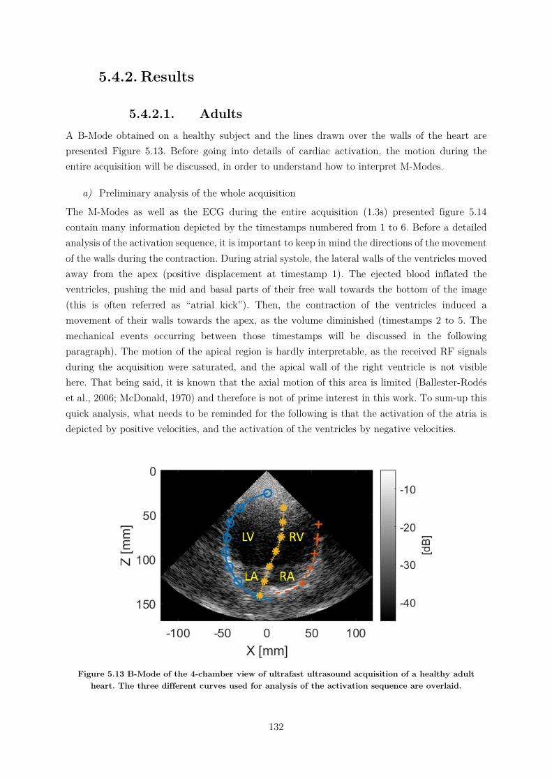
132

5.4.2. Results

5.4.2.1. Adults A B-Mode obtained on a healthy subject and the lines drawn over the walls of the heart are presented Figure 5.13. Before going into details of cardiac activation, the motion during the entire acquisition will be discussed, in order to understand how to interpret M-Modes.

a) Preliminary analysis of the whole acquisition

The M-Modes as well as the ECG during the entire acquisition (1.3s) presented figure 5.14 contain many information depicted by the timestamps numbered from 1 to 6. Before a detailed analysis of the activation sequence, it is important to keep in mind the directions of the movement of the walls during the contraction. During atrial systole, the lateral walls of the ventricles moved away from the apex (positive displacement at timestamp 1). The ejected blood inflated the ventricles, pushing the mid and basal parts of their free wall towards the bottom of the image (this is often referred as “atrial kick”). Then, the contraction of the ventricles induced a movement of their walls towards the apex, as the volume diminished (timestamps 2 to 5. The mechanical events occurring between those timestamps will be discussed in the following paragraph). The motion of the apical region is hardly interpretable, as the received RF signals during the acquisition were saturated, and the apical wall of the right ventricle is not visible here. That being said, it is known that the axial motion of this area is limited (Ballester-Rodés et al., 2006; McDonald, 1970) and therefore is not of prime interest in this work. To sum-up this quick analysis, what needs to be reminded for the following is that the activation of the atria is depicted by positive velocities, and the activation of the ventricles by negative velocities.

Figure 5.13 B-Mode of the 4-chamber view of ultrafast ultrasound acquisition of a healthy adult heart. The three different curves used for analysis of the activation sequence are overlaid.

133

b) Close-up analysis of activation sequence

Figure 5.15 shows the M-Modes of tissue velocities and accelerations zoomed-in around the activation of the heart. The atrial contraction started at t≈350ms (positive peak of acceleration at timestamp 1), followed by the activation of the ventricles at t=450ms (negative peak of acceleration, timestamp 2). The undesired effect of valves closure is clearly visible at t≈500ms (timestamp 3): the contraction of the ventricles caused the blood pressure to rise and when the pressure in the ventricles became higher than the pressure in the atria, the mitral and tricuspid valves were pushed and closed. The elastic waves generated are clearly visible on M-Modes. Finally, when the pressure in the ventricles were sufficient to open the pulmonary and aortic valves, the blood was ejected out of the ventricles. Their volume diminished as their walls moved toward the apex (timestamp 4). The crosses placed on the acceleration M-Modes indicates the measurements of the activation times of points along the walls.

The activation delays obtained are overlaid on the B-Mode image presented figure 5.16. Several conclusions can be drawn from these results. First of all, the lowest activation time was found to be in the atrial septum whereas it would be expected that the activation starts at the sinus node located in the right atrial wall: this suggest that the beginning of the atrial activation was missed, or in other words, that the total activation time is longer than what is found here. Secondly, the delay between the atrial and ventricular activations was 89ms, to be compared to the PR interval measureable on the ECG (here ~110ms): the shorter mechanical delay may come from the underestimated atrial activation time. Thirdly, the delays of the ventricular walls suggests that the activation went from the apex towards the basal sections of the wall, which is coherent with the implementation of Purkinje fibers discussed in the introduction of this chapter.

These results suggest that it is possible to provide a coarse cardiac activation sequence of the adult heart despite the increased difficulty brought by the in-vivo conditions. In the following section, the results obtained on fetal heart will be shown.

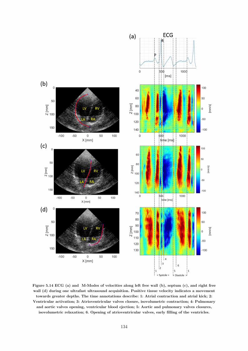
134

Figure 5.14 ECG (a) and M-Modes of velocities along left free wall (b), septum (c), and right free wall (d) during one ultrafast ultrasound acquisition. Positive tissue velocity indicates a movement towards greater depths. The time annotations describe: 1: Atrial contraction and atrial kick; 2:

Ventricular activation; 3: Atrioventricular valves closure, isovolumetric contraction; 4: Pulmonary and aortic valves opening, ventricular blood ejection; 5: Aortic and pulmonary valves closures, isovolumetric relaxation; 6. Opening of atrioventricular valves, early filling of the ventricles.

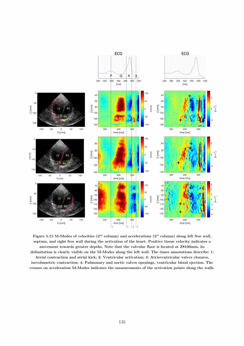
135

Figure 5.15 M-Modes of velocities (2nd column) and accelerations (3rd column) along left free wall, septum, and right free wall during the activation of the heart. Positive tissue velocity indicates a

movement towards greater depths. Note that the valvular floor is located at Z≈100mm, its delimitation is clearly visible on the M-Modes along the left wall. The times annotations describe: 1:

Atrial contraction and atrial kick; 2: Ventricular activation; 3: Atrioventricular valves closures, isovolumetric contraction; 4: Pulmonary and aortic valves openings, ventricular blood ejection. The

crosses on acceleration M-Modes indicates the measurements of the activation points along the walls.

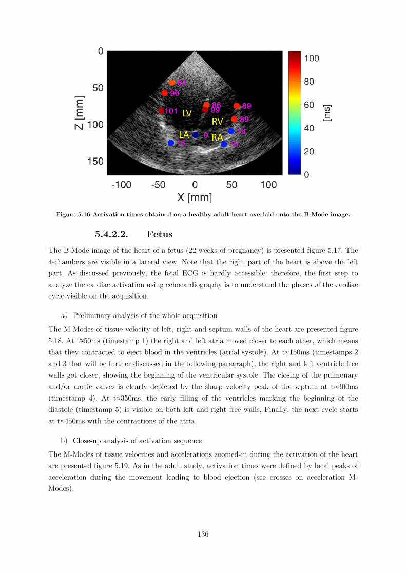
136

Figure 5.16 Activation times obtained on a healthy adult heart overlaid onto the B-Mode image.

5.4.2.2. Fetus The B-Mode image of the heart of a fetus (22 weeks of pregnancy) is presented figure 5.17. The 4-chambers are visible in a lateral view. Note that the right part of the heart is above the left part. As discussed previously, the fetal ECG is hardly accessible: therefore, the first step to analyze the cardiac activation using echocardiography is to understand the phases of the cardiac cycle visible on the acquisition.

a) Preliminary analysis of the whole acquisition

The M-Modes of tissue velocity of left, right and septum walls of the heart are presented figure 5.18. At t≈50ms (timestamp 1) the right and left atria moved closer to each other, which means that they contracted to eject blood in the ventricles (atrial systole). At t≈150ms (timestamps 2 and 3 that will be further discussed in the following paragraph), the right and left ventricle free walls got closer, showing the beginning of the ventricular systole. The closing of the pulmonary and/or aortic valves is clearly depicted by the sharp velocity peak of the septum at t≈300ms (timestamp 4). At t≈350ms, the early filling of the ventricles marking the beginning of the diastole (timestamp 5) is visible on both left and right free walls. Finally, the next cycle starts at t≈450ms with the contractions of the atria.

b) Close-up analysis of activation sequence

The M-Modes of tissue velocities and accelerations zoomed-in during the activation of the heart are presented figure 5.19. As in the adult study, activation times were defined by local peaks of acceleration during the movement leading to blood ejection (see crosses on acceleration M-Modes).

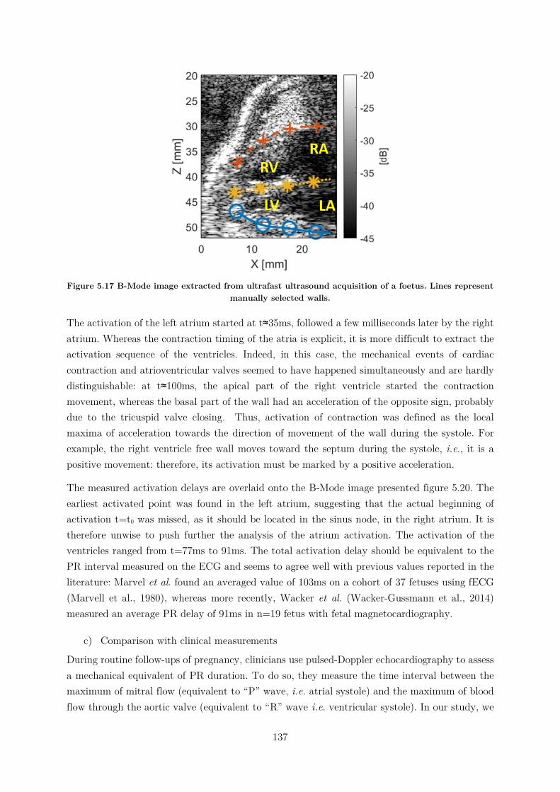
137

Figure 5.17 B-Mode image extracted from ultrafast ultrasound acquisition of a foetus. Lines represent

manually selected walls.

The activation of the left atrium started at t≈35ms, followed a few milliseconds later by the right atrium. Whereas the contraction timing of the atria is explicit, it is more difficult to extract the activation sequence of the ventricles. Indeed, in this case, the mechanical events of cardiac contraction and atrioventricular valves seemed to have happened simultaneously and are hardly distinguishable: at t≈100ms, the apical part of the right ventricle started the contraction movement, whereas the basal part of the wall had an acceleration of the opposite sign, probably due to the tricuspid valve closing. Thus, activation of contraction was defined as the local maxima of acceleration towards the direction of movement of the wall during the systole. For example, the right ventricle free wall moves toward the septum during the systole, i.e., it is a positive movement: therefore, its activation must be marked by a positive acceleration.

The measured activation delays are overlaid onto the B-Mode image presented figure 5.20. The earliest activated point was found in the left atrium, suggesting that the actual beginning of activation t=t0 was missed, as it should be located in the sinus node, in the right atrium. It is therefore unwise to push further the analysis of the atrium activation. The activation of the ventricles ranged from t=77ms to 91ms. The total activation delay should be equivalent to the PR interval measured on the ECG and seems to agree well with previous values reported in the literature: Marvel et al. found an averaged value of 103ms on a cohort of 37 fetuses using fECG (Marvell et al., 1980), whereas more recently, Wacker et al. (Wacker-Gussmann et al., 2014) measured an average PR delay of 91ms in n=19 fetus with fetal magnetocardiography.

c) Comparison with clinical measurements

During routine follow-ups of pregnancy, clinicians use pulsed-Doppler echocardiography to assess a mechanical equivalent of PR duration. To do so, they measure the time interval between the maximum of mitral flow (equivalent to “P” wave, i.e. atrial systole) and the maximum of blood flow through the aortic valve (equivalent to “R” wave i.e. ventricular systole). In our study, we

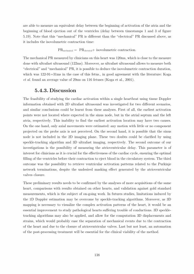
138

are able to measure an equivalent delay between the beginning of activation of the atria and the beginning of blood ejection out of the ventricles (delay between timestamps 1 and 3 of figure 5.19). Note that this “mechanical” PR is different than the “electrical” PR discussed above, as it includes the isovolumetric contraction time:

PRmechanical = PRelectrical+ isovolumetric contraction.

The mechanical PR measured by clinicians on this heart was 120ms, which is close to the measure done with ultrafast ultrasound (122ms). Moreover, as ultrafast ultrasound allows to measure both “electrical” and “mechanical” PR, it is possible to deduce the isovolumetric contraction duration, which was 122-91=31ms in the case of this fetus., in good agreement with the literature: Koga et al. found an average value of 29ms on 116 fetuses (Koga et al., 2001).

5.4.3. Discussion The feasibility of studying the cardiac activation within a single heartbeat using tissue Doppler information obtained with 2D ultrafast ultrasound was investigated for two different scenarios, and similar conclusions could be learnt from these analyses. First of all, the earliest activation points were not located where expected in the sinus node, but in the atrial septum and the left atria, respectively. This inability to find the earliest activation location may have two causes. On the one hand, only axial movements were estimated: any motion with little or no component projected on the probe axis is not perceived. On the second hand, it is possible that the sinus node is not included in the 2D imaging plane. These two doubts could be clarified by using speckle-tracking algorithm and 3D ultrafast imaging, respectively. The second outcome of our investigations is the possibility of measuring the atrioventricular delay. This parameter is of interest for clinicians as it is crucial for the effectiveness of the cardiac cycle, ensuring the optimal filling of the ventricles before their contraction to eject blood in the circulatory system. The third outcome was the possibility to retrieve ventricular activation patterns related to the Purkinje network terminations, despite the undesired masking effect generated by the atrioventricular valves closure.

These preliminary results needs to be confirmed by the analyses of more acquisitions of the same heart, comparisons with results obtained on other hearts, and validation against gold standard measurements, which is the subject of on-going work. In futures studies, limitations induced by the 1D Doppler estimation may be overcome by speckle-tracking algorithms. Moreover, as 3D mapping is necessary to visualize the complex activation patterns of the heart, it would be an essential improvement to study pathological hearts suffering trouble of conductions. 3D speckle-tracking algorithms may also be applied, and allow for the computation 3D displacements and strains, which would probably ease the separation of mechanical events due to the contraction of the heart and due to the closure of atrioventricular valves. Last but not least, an automation of the post-processing treatment will be essential for the clinical viability of the method.

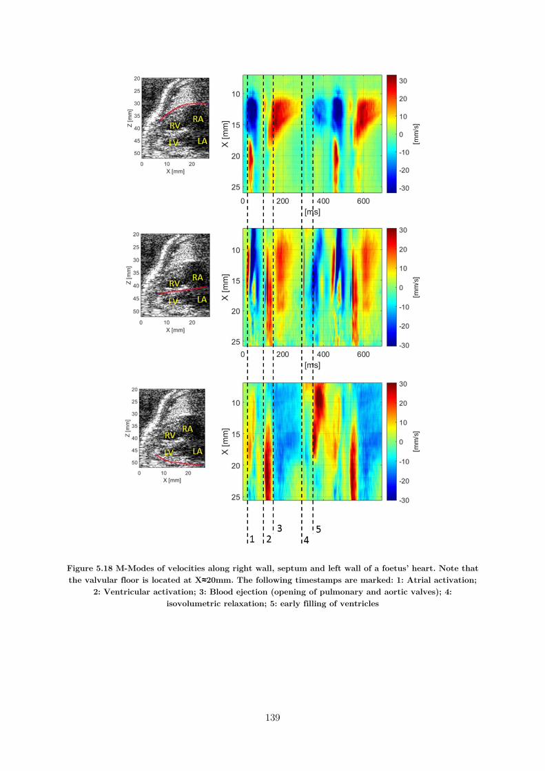
139

Figure 5.18 M-Modes of velocities along right wall, septum and left wall of a foetus’ heart. Note that the valvular floor is located at X≈20mm. The following timestamps are marked: 1: Atrial activation;

2: Ventricular activation; 3: Blood ejection (opening of pulmonary and aortic valves); 4: isovolumetric relaxation; 5: early filling of ventricles

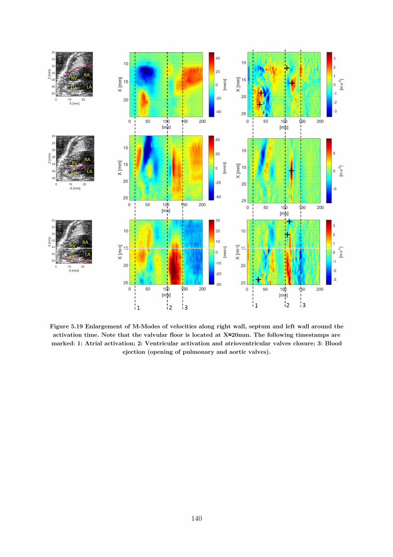
140

Figure 5.19 Enlargement of M-Modes of velocities along right wall, septum and left wall around the activation time. Note that the valvular floor is located at X≈20mm. The following timestamps are marked: 1: Atrial activation; 2: Ventricular activation and atrioventricular valves closure; 3: Blood

ejection (opening of pulmonary and aortic valves).

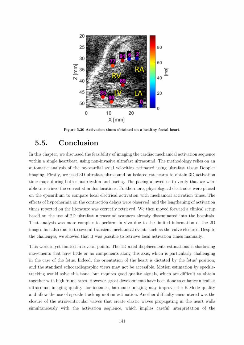
141

Figure 5.20 Activation times obtained on a healthy foetal heart.

5.5. Conclusion In this chapter, we discussed the feasibility of imaging the cardiac mechanical activation sequence within a single heartbeat, using non-invasive ultrafast ultrasound. The methodology relies on an automatic analysis of the myocardial axial velocities estimated using ultrafast tissue Doppler imaging. Firstly, we used 3D ultrafast ultrasound on isolated rat hearts to obtain 3D activation time maps during both sinus rhythm and pacing. The pacing allowed us to verify that we were able to retrieve the correct stimulus locations. Furthermore, physiological electrodes were placed on the epicardium to compare local electrical activation with mechanical activation times. The effects of hypothermia on the contraction delays were observed, and the lengthening of activation times reported on the literature was correctly retrieved. We then moved forward a clinical setup based on the use of 2D ultrafast ultrasound scanners already disseminated into the hospitals. That analysis was more complex to perform in vivo due to the limited information of the 2D images but also due to to several transient mechanical events such as the valve closures. Despite the challenges, we showed that it was possible to retrieve local activation times manually.

This work is yet limited in several points. The 1D axial displacements estimations is shadowing movements that have little or no components along this axis, which is particularly challenging in the case of the fetus. Indeed, the orientation of the heart is dictated by the fetus’ position, and the standard echocardiographic views may not be accessible. Motion estimation by speckle-tracking would solve this issue, but requires good quality signals, which are difficult to obtain together with high frame rates. However, great developments have been done to enhance ultrafast ultrasound imaging quality: for instance, harmonic imaging may improve the B-Mode quality and allow the use of speckle-tracking motion estimation. Another difficulty encountered was the closure of the atrioventricular valves that create elastic waves propagating in the heart walls simultaneously with the activation sequence, which implies careful interpretation of the

142

displacements. Strain-based algorithms may help to distinguish these two types of waves, but would require an improved signal-to-noise ratio. Moreover, the Purkinje network ends in multiple locations of the ventricles to insure the effectiveness of their contraction, which makes difficult the interpretation of 2D activation maps. Furthermore, when studying pathological cases, it will be of first importance to localize the defecting area: those two complications require necessarily 3D mapping. Once again, speckle-tracking algorithms would permit the estimation of 3D movements and strains, providing an extensive amount of information to analyze the contraction sequence. However, as of today, such algorithms face the challenges of relatively low quality of 3D images, and the high computational cost of such calculations.

143

5.6. Chapter Bibliography

Ballester-Rodés, M., Flotats, A., Torrent-Guasp, F., Carrió-Gasset, I., Ballester-Alomar, M., Carreras, F., Ferreira, A., Narula, J., 2006. The sequence of regional ventricular motion. European Journal of Cardio-Thoracic Surgery 29, S139–S144. https://doi.org/10.1016/j.ejcts.2006.02.058

Brooks, W., Bing, O., Blaustein, A., Allen, P., 1987. Comparison of contractile state and myosin isozymes of rat right and left ventricular myocardium*. Journal of Molecular and Cellular Cardiology 19, 433–440. https://doi.org/10.1016/S0022-2828(87)80395-4

Conrad, C.H., Brooks, W.W., Robinson, K.G., Bing, O.H., 1991. Impaired myocardial function in spontaneously hypertensive rats with heart failure. American Journal of Physiology-Heart and Circulatory Physiology 260, H136–H145. https://doi.org/10.1152/ajpheart.1991.260.1.H136

Delgado, V., Ypenburg, C., van Bommel, R.J., Tops, L.F., Mollema, S.A., Marsan, N.A., Bleeker, G.B., Schalij, M.J., Bax, J.J., 2008. Assessment of Left Ventricular Dyssynchrony by Speckle Tracking Strain Imaging. Journal of the American College of Cardiology 51, 1944–1952. https://doi.org/10.1016/j.jacc.2008.02.040

D’hooge, J., 2000. Regional Strain and Strain Rate Measurements by Cardiac Ultrasound: Principles, Implementation and Limitations. European Journal of Echocardiography 1, 154–170. https://doi.org/10.1053/euje.2000.0031

Dick, D., 1998. Mechanical modulation of stretch-induced premature ventricular beats: induction of a mechanoelectric adaptation period. Cardiovascular Research 38, 181–191. https://doi.org/10.1016/S0008-6363(97)00314-3

Eliasson, H., Sonesson, S.-E., Sharland, G., Granath, F., Simpson, J.M., Carvalho, J.S., Jicinska, H., Tomek, V., Dangel, J., Zielinsky, P., Respondek-Liberska, M., Freund, M.W., Mellander, M., Bartrons, J., Gardiner, H.M., for the Fetal Working Group of the European Association of Pediatric Cardiology, 2011. Isolated Atrioventricular Block in the Fetus: A Retrospective, Multinational, Multicenter Study of 175 Patients. Circulation 124, 1919–1926. https://doi.org/10.1161/CIRCULATIONAHA.111.041970

Faris, O.P., Evans, F.J., Ennis, D.B., Helm, P.A., Taylor, J.L., Chesnick, A.S., Guttman, M.A., Ozturk, C., McVeigh, E.R., 2003. Novel Technique for Cardiac Electromechanical Mapping with Magnetic Resonance Imaging Tagging and an Epicardial Electrode Sock. Annals of Biomedical Engineering 31, 430–440. https://doi.org/10.1114/1.1560618

Geyer, H., Caracciolo, G., Abe, H., Wilansky, S., Carerj, S., Gentile, F., Nesser, H.-J., Khandheria, B., Narula, J., Sengupta, P.P., 2010. Assessment of Myocardial Mechanics Using Speckle Tracking Echocardiography: Fundamentals and Clinical Applications.

144

Journal of the American Society of Echocardiography 23, 351–369. https://doi.org/10.1016/j.echo.2010.02.015

Gorcsan, J., Abraham, T., Agler, D.A., Bax, J.J., Derumeaux, G., Grimm, R.A., Martin, R., Steinberg, J.S., Sutton, M.S.J., Yu, C.-M., 2008. Echocardiography for Cardiac Resynchronization Therapy: Recommendations for Performance and Reporting–A Report from the American Society of Echocardiography Dyssynchrony Writing Group Endorsed by the Heart Rhythm Society. Journal of the American Society of Echocardiography 21, 191–213. https://doi.org/10.1016/j.echo.2008.01.003

Herron, T.J., Lee, P., Jalife, J., 2012. Optical Imaging of Voltage and Calcium in Cardiac Cells & Tissues. Circulation Research 110, 609–623. https://doi.org/10.1161/CIRCRESAHA.111.247494

Kasai, C., NAMEKAWA, K., KOYANO, A., OMOTO, R., 1985. Real-Time Two-Dimensional Blood Flow Imaging Using an Autocorrelation Technique 7.

Koga, T., Athayde, N., Trudinger, B., 2001. The fetal cardiac isovolumetric contraction time in normal pregnancy and in pregnancy with placental vascular disease: the first clinical report using a new ultrasound technique. BJOG: An International Journal of Obstetrics and Gynaecology 108, 179–185. https://doi.org/10.1111/j.1471-0528.2001.00033.x

Konofagou, E.E., Luo, J., Saluja, D., Cervantes, D.O., Coromilas, J., Fujikura, K., 2010. Noninvasive electromechanical wave imaging and conduction-relevant velocity estimation in vivo. Ultrasonics 50, 208–215. https://doi.org/10.1016/j.ultras.2009.09.026

Konofagou, E.E., Provost, J., 2012. Electromechanical wave imaging for noninvasive mapping of the 3D electrical activation sequence in canines and humans in vivo. Journal of Biomechanics 45, 856–864. https://doi.org/10.1016/j.jbiomech.2011.11.027

Langendorff, O., 1895. Untersuchungen am überlebenden Säugethierherzen. Archiv für die gesamte Physiologie des Menschen und der Tiere 61, 291–332.

Luo, J., Bai, J., He, P., Ying, K., 2004. Axial strain calculation using a low-pass digital differentiator in ultrasound elastography. IEEE transactions on ultrasonics, ferroelectrics, and frequency control 51, 1119–1127.

Malmivuo, J., Plonsey, R., 1995. BioelectromagnetismPrinciples and Applications of Bioelectric and Biomagnetic Fields. Oxford University Press. https://doi.org/10.1093/acprof:oso/9780195058239.001.0001

Marian, A.J., Wu, Y., Lim, D.-S., McCluggage, M., Youker, K., Yu, Q., Brugada, R., DeMayo, F., Quinones, M., Roberts, R., 1999. A transgenic rabbit model for human hypertrophic cardiomyopathy. Journal of Clinical Investigation 104, 1683–1692. https://doi.org/10.1172/JCI7956

145

Marvell, C.J., Kirk, D.L., Jenkins, H.M.L., Symonds, E.M., 1980. THE NORMAL CONDITION OF THE FETAL ELECTROCARDIOGRAM DURING LABOUR. BJOG: An International Journal of Obstetrics and Gynaecology 87, 786–796. https://doi.org/10.1111/j.1471-0528.1980.tb04614.x

Matiukas, A., Mitrea, B.G., Qin, M., Pertsov, A.M., Shvedko, A.G., Warren, M.D., Zaitsev, A.V., Wuskell, J.P., Wei, M., Watras, J., Loew, L.M., 2007. Near-infrared voltage-sensitive fluorescent dyes optimized for optical mapping in blood-perfused myocardium. Heart Rhythm 4, 1441–1451. https://doi.org/10.1016/j.hrthm.2007.07.012

McDonald, I.G., 1970. The shape and movements of the human left ventricle during systole. The American Journal of Cardiology 26, 221–230. https://doi.org/10.1016/0002-9149(70)90787-3

Nash, M.P., Pullan, A.J., 2005. Challenges Facing Validation of Noninvasive Electrical Imaging of the Heart. Annals of Noninvasive Electrocardiology 10, 73–82. https://doi.org/10.1111/j.1542-474X.2005.00608.x

Nauleau, P., Melki, L., Wan, E., Konofagou, E., 2017. A 3-D rendering algorithm for Electromechanical Wave Imaging of a beating heart. Medical Physics.

Notabartolo, D., Merlino, J.D., Smith, A.L., DeLurgio, D.B., Vera, F.V., Easley, K.A., Martin, R.P., León, A.R., 2004. Usefulness of the peak velocity difference by tissue Doppler imaging technique as an effective predictor of response to cardiac resynchronization therapy. The American Journal of Cardiology 94, 817–820. https://doi.org/10.1016/j.amjcard.2004.05.072

Nygren, A., Clark, R.B., Belke, D.D., Kondo, C., Giles, W.R., Witkowski, F.X., 2000. Voltage-Sensitive Dye Mapping of Activation and Conduction in Adult Mouse Hearts. Annals of Biomedical Engineering 28, 958–967. https://doi.org/10.1114/1.1308501

Nygren, A., Kondo, C., Clark, R.B., Giles, W.R., 2003. Voltage-sensitive dye mapping in Langendorff-perfused rat hearts. American Journal of Physiology - Heart and Circulatory Physiology 284, H892–H902. https://doi.org/10.1152/ajpheart.00648.2002


Pernot, M., Konofagou, E.E., 2005. Electromechanical imaging of the myocardium at normal and pathological states. IEEE, pp. 1091–1094. https://doi.org/10.1109/ULTSYM.2005.1603040


146

Provost, J., Wei-Ning Lee, Fujikura, K., Konofagou, E.E., 2010. Electromechanical Wave Imaging of Normal and Ischemic Hearts In Vivo. IEEE Transactions on Medical Imaging 29, 625–635. https://doi.org/10.1109/TMI.2009.2030186

Ramanathan, C., 2006. Noninvasive 3D imaging of electrophysiological activity in the heart. SPIE Newsroom. https://doi.org/10.1117/2.1200605.0247

Ramanathan, C., Ghanem, R.N., Jia, P., Ryu, K., Rudy, Y., 2004. Noninvasive electrocardiographic imaging for cardiac electrophysiology and arrhythmia. Nature Medicine 10, 422–428. https://doi.org/10.1038/nm1011

Rosenbaum, D.S., Girouard, S.D., Laurita, K.R., 1992. High resolution cardiac mapping with voltage sensitive dyes. IEEE, pp. 1995–1996. https://doi.org/10.1109/IEMBS.1992.5762137

Salama, G., Morad, M., 1976. Merocyanine 540 as an optical probe of transmembrane electrical activity in the heart. Science 191, 485–487. https://doi.org/10.1126/science.191.4226.485

Sameni, 2010. A Review of Fetal ECG Signal Processing Issues and Promising Directions. The Open Pacing, Electrophysiology & Therapy Journal. https://doi.org/10.2174/1876536X01003010004

Skrzypiec-Spring, M., Grotthus, B., Szeląg, A., Schulz, R., 2007. Isolated heart perfusion according to Langendorff—Still viable in the new millennium. Journal of Pharmacological and Toxicological Methods 55, 113–126. https://doi.org/10.1016/j.vascn.2006.05.006

Smeets, J.L., Allessie, M.A., Lammers, W.J., Bonke, F.I., Hollen, J., 1986. The wavelength of the cardiac impulse and reentrant arrhythmias in isolated rabbit atrium. The role of heart rate, autonomic transmitters, temperature, and potassium. Circulation Research 58, 96–108. https://doi.org/10.1161/01.RES.58.1.96

Suffoletto, M.S., 2006. Novel Speckle-Tracking Radial Strain From Routine Black-and-White Echocardiographic Images to Quantify Dyssynchrony and Predict Response to Cardiac Resynchronization Therapy. Circulation 113, 960–968. https://doi.org/10.1161/CIRCULATIONAHA.105.571455

van der Linde, D., Konings, E.E.M., Slager, M.A., Witsenburg, M., Helbing, W.A., Takkenberg, J.J.M., Roos-Hesselink, J.W., 2011. Birth Prevalence of Congenital Heart Disease Worldwide. Journal of the American College of Cardiology 58, 2241–2247. https://doi.org/10.1016/j.jacc.2011.08.025

van Engelen, A.D., Weijtens, O., Brenner, J.I., Kleinman, C.S., Copel, J.A., Stoutenbeek, P., Meijboom, E.J., 1994. Management outcome and follow-up of fetal tachycardia. Journal of the American College of Cardiology 24, 1371–1375. https://doi.org/10.1016/0735-1097(94)90122-8

147

Wacker-Gussmann, A., Paulsen, H., Stingl, K., Braendle, J., Goelz, R., Henes, J., 2014. Atrioventricular Conduction Delay in the Second Trimester Measured by Fetal Magnetocardiography. Journal of Immunology Research 2014, 1–6. https://doi.org/10.1155/2014/753953

Wyman, B.T., Hunter, W.C., Prinzen, F.W., McVeigh, E.R., 1999. Mapping propagation of mechanical activation in the paced heart with MRI tagging. American Journal of Physiology-Heart and Circulatory Physiology 276, H881–H891. https://doi.org/10.1152/ajpheart.1999.276.3.H881

Zhang, X., Ramachandra, I., Liu, Z., Muneer, B., Pogwizd, S.M., He, B., 2005. Noninvasive three-dimensional electrocardiographic imaging of ventricular activation sequence. American Journal of Physiology-Heart and Circulatory Physiology 289, H2724–H2732. https://doi.org/10.1152/ajpheart.00639.2005

149

: Conclusion

This thesis was focused on 3D ultrafast ultrasound imaging of the heart for the characterisation of cardiac tissues’ properties. In order to do so, a real-time imaging modality was developed on a 1024-channel ultrafast ultrasound system, and dedicated 3D and 4D visualization tools were developed. This system is highly versatile and has the capability to perform fundamental research on small animals but also clinical studies on human patients. This work has enhanced the utilisation of the 3D ultrafast ultrasound scanner built in our lab and is being used within our group for other research applications on other organs such as the brain or the liver which are not presented in this manuscript.

Then, we presented 3D Backscatter Tensor Imaging (BTI), an application dedicated to the imaging of the fibres architecture of the human heart in-vivo and non-invasively during the cardiac cycle. The effect of axial motion on the technique was investigated, and a solution to estimate its velocity and reduce the undesired artefacts was introduced. BTI could become a tool of choice to measure the microstructural anisotropy of soft tissues, and find clinical applications in the study of cardiac pathologies implying fibre disarray (such as hypertrophic cardiomyopathies), or research applications to image the fibrous structure of the brain.

Afterward, we introduced a framework dedicated to the imaging of naturally generated elastic waves propagating in the human heart walls during the cardiac cycle, as well as a methodology to measure their speed. Future developments will be focused on the retrieval of the heart elasticity from these measurements, which would allow to assess the myocardial stiffness during both contraction and relaxation.

Last but not least, we performed the imaging of the cardiac contraction in 3D on isolated rat hearts in order to analyse the synchronisation of the cardiac activation. The activation sequences could be retrieved during the natural rhythm of the heart, under pacing conditions and hypothermia. Finally, the application of the technique in 2D in a clinical setting was investigated on foetuses and adults human hearts. The perspectives of this work are to enhance and facilitate the detection and localization of cardiac arrhythmias, for their better treatment.

Note that the fibrous texture of the heart impacts directly the velocity of elastic waves within the heart walls as well as the activation contraction sequence: both of these phenomenon propagate preferably along the directions of the fibres rather than perpendicularly. Thus in future studies, it would be interesting to combine the three techniques developed during this PhD and compare, from a single 3D ultrafast ultrasound acquisition during one heartbeat, the orientation of cardiac fibres, the velocity of elastic waves naturally propagating and their anisotropy, and the cardiac activation sequence.

In general, the techniques developed in this PhD hope to set back the limitations of conventional echocardiography while maintaining its advantages, and may find clinical applications in order

150

to better diagnose and/or follow-up cardiac pathologies. Indeed, it may be possible in the future to assess at the bed side of the patient new properties such as the myocardial stiffness, the myocardial fibers organization, or the precise mechanical activation sequence. Thus, future work should also focus on clinical studies to evaluate the benefits of using 3D ultrafast imaging in a various set of pathological cases. As of today, the availability of 3D ultrafast ultrasound scanners and fully populated matrix probes remains limited to a few research centres, and these material remain expensive and bulky. However, future technologies will shortly provide solutions to reduce both their costs and size: in particular, current researches aim to reduce the numbers of channels of the 3D probes, either by using sparse arrays, raw-column arrays, or integrating micro-beamformers within the probe. Hence, it is reasonable to think that 3D ultrafast ultrasound imaging could become a standard clinical equipment in a few decades.

151

Scientific output

Publications in peer-reviewed journals

C. Papadacci**, V. Finel**, J. Provost, O. Villemain, P. Bruneval, J.-L. Gennisson, M. Tanter, M. Fink, M. Pernot, 2017. Imaging the dynamics of cardiac fiber orientation in vivo using 3D Ultrasound Backscatter Tensor Imaging. Scientific Reports 7 https://doi.org/10.1038/s41598-017-00946-7 (**co-first authors)

C. Papadacci, V. Finel, E. Cohen, O. Villemain, J. Provost, M. Tanter and M. Pernot, Simultaneous 4D ultrafast blood flow and tissue Doppler imaging of the human heart to retrieve every quantification parameters in one acquisition (submitted)

V. Finel, C. Papadacci, E. Cohen, M. Tanter, M. Pernot, 4D cardiac ultrafast imaging of natural mechanical waves: towards quantitative elastography of the human ventricle (in preparation)

V. Finel, P. Mateo, C. Papadacci, J. Provost, M. Tanter, M. Pernot, 4D ultrafast imaging of myocardial contraction activation in normal and pathological isolated rat hearts (in preparation)

V. Finel, C. Papadacci, J. Provost, M. Tanter and M. Pernot, Motion Correction for 3D Ultrafast Ultrasound: Application to 3D Backscattered Tensor Imaging of Soft Tissues Anisotropy (in preparation)

C. Rabut, M. Correia, V. Finel, S. Pezet, M. Pernot, T. Deffieux, M. Tanter, 4D functional ultrasound imaging of whole-brain activity in rodents (in preparation)

Peer-reviewed abstracts

C. Papadacci, V. Finel, J. Provost, M. Tanter, M. Pernot, Mapping myocardial fiber orientation using ultrasound Backscatter tensor imaging, TOPIM 2016, 2016, Les Houches, France

V. Finel, C. Papadacci, J. Provost, M. Tanter, M. Pernot, Mapping myocardial fiber orientation using ultrasound Backscatter tensor imaging, CNIV 2016, 2016, Paris, France

V. Finel, C. Papadacci, J. Provost, M. Tanter, M. Pernot, Mapping of myocardial fiber orientation using ultrasound Backscatter tensor imaging in ex vivo myocardium and in the human beating heart, IEEE IUS 2016, 2016, Tours, France

C. Rabut, M. Correia, V. Finel, T. Deffieux, M. Pernot, and M. Tanter, Full 3D dynamic functional ultrasound imaging of neuronal activity in mice, Acoustics ‘17 Boston, 2017, Boston, USA

V. Finel, C. Papadacci, O. Villemain, J. Provost, M. Tanter, M. Pernot, Mapping of myocardial fiber orientation using ultrasound Backscatter tensor imaging in the human beating heart, WMIC 2017, 2017, Köln, Germany

152

C. Rabut, V. Finel, M. Correia, M. Pernot, T. Deffieux and M. Tanter, Full 4D Functional Ultrasound Imaging in Rodents Using a Matrix Array, IEEE IUS 2017, 2017, Washington DC, USA

V. Finel, P. Mateo, C. Papadacci, J. Provost, M. Tanter and M. Pernot, 3D Ultrafast Imaging of the Heart: Application to the Mapping of Electromechanical Activation, IEEE IUS 2017, 2017, Washington DC, USA

V. Finel, C. Papadacci, J. Provost, M. Tanter and M. Pernot, Motion Correction for 3D Ultrafast Ultrasound: Application to 3D Backscattered Tensor Imaging of Soft Tissues Anisotropy, IEEE IUS 2017, 2017, Washington DC, USA

V. Finel, C. Papadacci, O. Villemain, J. Provost, M. Tanter, M. Pernot, Imaging of cardiac fibers orientation in vivo using 3D Ultrasound Backscatter Imaging in the human beating heart, WMIC 2017, 2017 Washington DC, USA

V. Finel, P. Mateo, C. Papadacci, J. Provost, M. Tanter, M. Pernot, 3D mapping of cardiac contraction on isolated rat heart using ultrasound ultrafast imaging, EMIM 2018, 2018, San Sebastian, Spain (best poster award)

V. Finel, P. Mateo, C. Papadacci, J. Provost, M. Tanter, M. Pernot, 4D ultrafast imaging of myocardial contraction activation in normal and pathological isolated rat hearts, IEEE IUS 2018, 2018, Kobe, Japan

V. Finel, C. Papadacci, E. Cohen, M. Tanter and M. Pernot, 4D cardiac ultrafast imaging of natural mechanical waves: towards quantitative elastography of the human ventricle, IEEE IUS 2018, 2018, Kobe, Japan

C. Rabut, V. Finel, M. Correia, M. Pernot, T. Deffieux, M. Tanter, 3D Multiplane Wave imaging in ultrafast ultrasound allowing 4D NeuroFunctional Ultrasound imaging for 3D fast events tracking and 3D connectivity mapping, IEEE IUS 2018, 2018, Kobe, Japan

C. Papadacci, V. Finel, O. Villemain, G. Goudot, J. Provost, M. Tanter and M. Pernot, Simultaneous 4D ultrafast blood flow and tissue Doppler imaging of the human heart, IEEE IUS 2018, 2018, Kobe, Japan

C. Rabut, V. Finel, M. Correia, M. Pernot, T. Deffieux, M. Tanter, 4D neurofunctional ultrasound imaging in rodents allowing highly resolved 3D tracking of fast events and 3D connectivity mapping, SFN Meeting 2018, 2018, San Diego, USA

153

Awards

EMIM 2018 poster award in the category cardiovascular imaging I, EMIM 2018, San Sebastian, Spain

Documents

3D ultrafast echocardiography: toward a quantitative