3D Tumor Segmentation from Volumetric Brain MR Images ...cdn.intechweb.org/pdfs/20267.pdf · 3D Tumor Segmentation from Volumetric Brain ... of neuro-imaging, ... 3D Tumor Segmentation

6

3D Tumor Segmentation from Volumetric Brain MR Images Using Level-Sets Method

Kamel Aloui and Mohamed Saber Naceur National Engineering School, LTSIRS Laboratory – Tunis

Tunisia

1. Introduction

1.1 Statement of the problem Segmentation in volumetric images is a tool allowing a diagnostics automation and as well will assist experts in quantitative and qualitative analysis. It’s an important step in various applications such as visualization, morphometrics and image-guided surgery. In the context of neuro-imaging, brain tumor segmentation from Magnetic Resonance Images (MRI) is extremely important for treatment planning, therapy monitoring, examining efficacy of radiation and drug treatments and studying the difference between healthy subjects and subjects with brain tumor. The task of manually segmentation of brain tumor from MR images is generally time-consuming and difficult. Anyway, the task is done by marking by hand the tumor regions slice-by-slice which generates set of jaggy images, so the practitioner is confronted with a succession of boundary which he mentally stacked up to be made a 3D shape of brain tumor. This shape is inevitably subjective and becomes infeasible when dealing with large data sets, also there is losing of information in the third dimension because is not taken into account in the segmentation process. All this, affect the quality and accuracy of clinical diagnosis. An automatic or semi-automatic segmentation method of brain tumor that takes entire information within the volumetric MR image into account is desirable as it reduces the load on the human raters and generates optimal segmented images (Wang & al., 2004), (Michael & al., 2001), (Lynn & al., 2001). Specially, automatic brain tumor segmentation presents many challenges and involves various disciplines such us pathology, MRI physics and image processing. Brain tumors are difficult to segment because they vary greatly in size and position, may be of any size, may have a variety of shapes and may have overlapping intensities with normal tissue and edema. This leads to numerous segmentation approaches of automatic brain tumor extraction. Low-level segmentation methods, such as pixel-based clustering, region growing, and filter-based edge detection, requires additional pre-processing and post-processing as well as considerable amounts of expert intervention and a priori knowledge on the regions of interest (ROI) (Sahoo & al., 1988). Recently, several attempts have been made to apply deformable models to brain image analysis (Moon & al., 2002). Indeed, deformable models refer to a large class of computer vision methods and have proved to be a successful segmentation technique for a wide range of applications. Deformable models, on the other hand, provide an explicit representation of the boundary and the ROI shape. They combine several desirable features such as inherent connectivity and smoothness, which counteract

www.intechopen.com

Diagnostic Techniques and Surgical Management of Brain Tumors

118

noise and boundary irregularities, as well as the ability to incorporate knowledge about the ROI. However, parametric deformable model must be re-parameterized dynamically to recover the object boundary and that has difficulty in dealing with topological adaptation such as splitting or merging model parts. A level-Sets deformable model, also referred to as a geometric deformable model, provides an elegant solution to address the primary limitations of parametric deformable models (Taheri & al., 2009), (Taheri & al., 2007), (Lefohn & al., 2003). These methods have drawn a great deal of attention since their introduction in 1988. Advantages of the contour implicit formulation of the deformable model over parametric formulation include: no parameterization of the contour, topological flexibility, good numerical stability and straightforward extension of the 2D formulation to n-D.

1.2 Outline of our method In this work, we describe various segmentation tools for segmenting brain tumor from

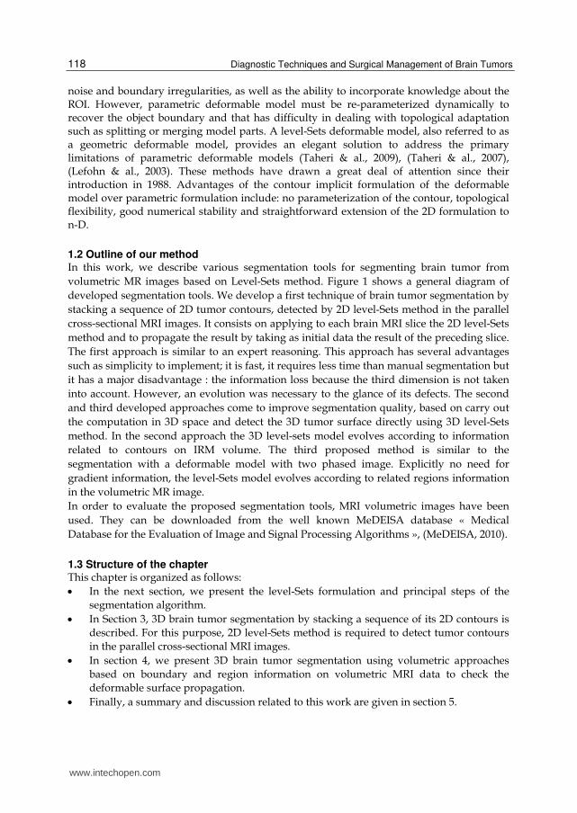
volumetric MR images based on Level-Sets method. Figure 1 shows a general diagram of

developed segmentation tools. We develop a first technique of brain tumor segmentation by

stacking a sequence of 2D tumor contours, detected by 2D level-Sets method in the parallel

cross-sectional MRI images. It consists on applying to each brain MRI slice the 2D level-Sets

method and to propagate the result by taking as initial data the result of the preceding slice.

The first approach is similar to an expert reasoning. This approach has several advantages

such as simplicity to implement; it is fast, it requires less time than manual segmentation but

it has a major disadvantage : the information loss because the third dimension is not taken

into account. However, an evolution was necessary to the glance of its defects. The second

and third developed approaches come to improve segmentation quality, based on carry out

the computation in 3D space and detect the 3D tumor surface directly using 3D level-Sets

method. In the second approach the 3D level-sets model evolves according to information

related to contours on IRM volume. The third proposed method is similar to the

segmentation with a deformable model with two phased image. Explicitly no need for

gradient information, the level-Sets model evolves according to related regions information

in the volumetric MR image.

In order to evaluate the proposed segmentation tools, MRI volumetric images have been

used. They can be downloaded from the well known MeDEISA database « Medical

Database for the Evaluation of Image and Signal Processing Algorithms », (MeDEISA, 2010).

1.3 Structure of the chapter This chapter is organized as follows:

In the next section, we present the level-Sets formulation and principal steps of the

segmentation algorithm.

In Section 3, 3D brain tumor segmentation by stacking a sequence of its 2D contours is

described. For this purpose, 2D level-Sets method is required to detect tumor contours

in the parallel cross-sectional MRI images.

In section 4, we present 3D brain tumor segmentation using volumetric approaches

based on boundary and region information on volumetric MRI data to check the

deformable surface propagation.

Finally, a summary and discussion related to this work are given in section 5.

www.intechopen.com


119

Fig. 1. General diagram of developed segmentation tools for segmenting 3D brain tumor from volumetric MR images based on Level-Sets method.

2. Level-set method: Presentation

In this Section, we describe a modeling technique based on a level-Sets approach for recovering shapes of objects in two and three dimensions. The modeling technique may be viewed as a form of active modeling such as “snakes” (Kass & al., 1988) and deformable surfaces (Terzopoulos & al. 1988). The model which consists of a moving front, until is plated on the desired shape, by externally applied stop criteria synthesized from the image data (Fig. 2.). Specially, deformable models are curves or surfaces defined in a digital image that can move under the influence of external and internal forces. External forces, which are computed from the image data, are designed to keep the model smooth during deformations. The external forces are defined from the deformable curve or surface like

www.intechopen.com


120

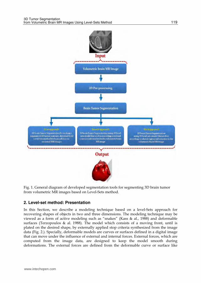
curvature in order to move the model to the boundary of a region of interest (ROI) in the digital image. Using these two forces, deformable models offer robustness to both image noise and boundary gaps, by constraining extracted ROI’s boundaries to be smooth and incorporating other prior information about the ROI shape. Moreover, the resulting boundary representation can achieve subpixel accuracy which is considered a highly desirable property for medical imaging applications.

a) b) c) d)

Fig. 2. Principle of deformable curve in two space dimensions. We show curve evolution in time.

There are basically two types of deformable models:

Parametric deformable models (Kass & al., 1988), (Amini & al., 1990), (Cohen, 1991) and (McInerney & al., 1995);

Geometric deformable models (Caselles & al., 1993), (Milladi & al., 1995), (Caselles & al., 1995) and (Whitaker, 1994).

Parametric deformable models represent curves and surfaces explicitly in their parametric forms during deformation. This representation allows direct interaction with the model and can lead to a compact representation for fast real-time implementation. Adaptation of the model topology such as splitting or merging parts during the deformation can be difficult using parametric models. However, geometric deformable models can handle topological changes naturally. These models, based on the theory of curve evolution (Sapiro & Tannenbaum, 1993), (Kimia & al., 1995), (Kimmel & al., 1995), (Alvarez & al., 1993) and the level set method (Osher & Sethian, 1988), (Sethian, 1999) represent curves and surfaces implicitly as a level-Sets of a higher-dimensional scalar function. Their parameterizations are computed only after complete deformation, thereby allowing topological adaptively to be easily accommodated. Despite this fundamental difference, the principles of both methods are very similar. Level-Sets method as a geometric deformable model; provide an elegant solution to address the primary limitations of parametric deformable models. In particular, curves and surfaces move using only geometric measures and other prior information from the image data to recover ROI boundaries. In this section, we first review the fundamental concepts in curve evolution theory and the level-Sets method.

2.1 Curve evolution theory The purpose of curve evolution theory is to study the deformation of curves using only geometric measures such as the curvature and the unit normal. Let us consider a moving

curve t , where t represents the time;

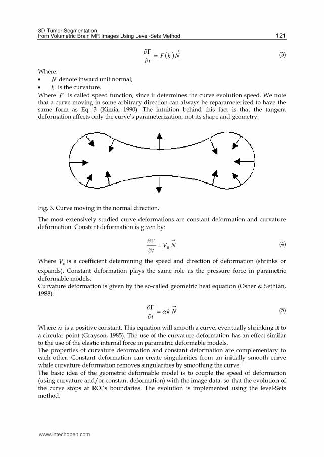
The evolution of the curve along its normal direction can be characterized by the following partial differential equation (Fig. 3.):

www.intechopen.com


121

NkFt

(3)

Where:

N denote inward unit normal;

k is the curvature. Where F is called speed function, since it determines the curve evolution speed. We note that a curve moving in some arbitrary direction can always be reparameterized to have the same form as Eq. 3 (Kimia, 1990). The intuition behind this fact is that the tangent deformation affects only the curve’s parameterization, not its shape and geometry.

Fig. 3. Curve moving in the normal direction.

The most extensively studied curve deformations are constant deformation and curvature deformation. Constant deformation is given by:

NV

t0

(4)

Where 0V is a coefficient determining the speed and direction of deformation (shrinks or

expands). Constant deformation plays the same role as the pressure force in parametric deformable models. Curvature deformation is given by the so-called geometric heat equation (Osher & Sethian, 1988):

Nk

t (5)

Where is a positive constant. This equation will smooth a curve, eventually shrinking it to

a circular point (Grayson, 1985). The use of the curvature deformation has an effect similar to the use of the elastic internal force in parametric deformable models. The properties of curvature deformation and constant deformation are complementary to each other. Constant deformation can create singularities from an initially smooth curve while curvature deformation removes singularities by smoothing the curve. The basic idea of the geometric deformable model is to couple the speed of deformation

(using curvature and/or constant deformation) with the image data, so that the evolution of

the curve stops at ROI’s boundaries. The evolution is implemented using the level-Sets

method.

www.intechopen.com


122

2.2 Level-Sets method: Basic algorithms

We now review the level-Sets method for implementing curve evolution. The level-Sets

method is used to account for automatic topology adaptation, and it also provides the basis

for a numerical scheme that is used by geometric deformable models. The level-Sets method

for evolving curves is due to Osher and Sethian (Osher & Sethian, 1988), (Sethian, 1985) and

(Sethian, 1989). The interface bounds a (possibly multiply connected) region . The goal

is to compute and analyze the subsequent motion of under a velocity field F . This

velocity can depend on position X (Where yxX , in tow space dimensions or zyxX ,, in three space dimensions), time, the geometry of the interface and the

external physics. The interface is captured as the zero level-Sets of a smooth function:

tX , , i.e., 0, tXXt (6)

is positive inside , negative outside and is zero on t , has the following

properties:

TXfortX

XfortX

XfortX

0,

0,

0,

(7)

Thus, the interface is to be captured for all later time, by merely locating the set t for

which vanishes.

We note that the only purpose of the level-Sets function is to provide an implicit

representation of the evolving curve and the topological merging and breaking are well

defined and easily performed. Instead of tracking a curve through time, the level-Sets

method evolves a curve by updating the level-Sets function at fixed coordinates through

time. A useful property of this approach is that the level-Sets function remains a valid

function while the embedded curve can change its topology. The motion is analyzed by

convecting the values (levels) with the velocity field F . This elementary equation is:

0

kFt

(8)

Where denotes the gradient of .

Here F is the desired velocity on the interface, and is arbitrary elsewhere. Actually, only the normal component of F is needed. The inward unit normal to the level-Sets curve is given by:

N (9)

Then

kFkFN (10)

www.intechopen.com


123

Accordingly, Eq. 8 becomes

0

kFt

N (11)

Finally, the curvature k at the zero level-Sets is given by:

32

22

222

yx

xyyxyyxyxxdivk

(12)

2.3 Level-sets: Speed function The geometric deformable contour formulation, proposed in (Caselles & al., 1993) and

(Malladi & al., 1995), takes the following form:

kVIgkFt

N 0 (13)

Where

p

I

Igˆ1

1

(14)

Positive 0V shrinks the curve, and negative

0V expands the curve. The curve evolution is

coupled with the image data through a multiplicative stopping term Ig . Where I is the

image corrected by a Gaussian operator and 21 orp . This scheme can work well for

objects that have good contrast. However, when the object boundary is indistinct or has

gaps, the geometric deformable contour may leak out because the multiplicative term only

slows down the curve near the boundary rather than completely stopping the curve. Once

the curve passes the boundary, it will not be pulled back to recover the correct boundary.

2.4 Level-Sets: Numerical implementation Various numerical implementations of deformable models have been reported in the literature. For examples, the finite difference method (Kass & al., 1988), dynamic programming (Amini & al., 1990), and greedy algorithm (Williams & Shah, 1992) have been used. In this section, we present the finite difference method implementation for level-Sets method as described in (Kass & al., 1988).

2.4.1 Initialization

An initial function 0, tX must be constructed such that its zero level-Sets correspond

to the position of the initial contour or surface. A common choice is to set:

xdtX 0, (15)

Where xd is the signed distance from each grid point to the zero level-Sets. For example, when the zero level-Sets can be described by the exterior boundary of a circle, the signed distance function can be computed as follows:

www.intechopen.com


124

ryyxxtyx 2

0

2

00,, (16)

Where 000 , yxX is the center and r is the radius of the circle.

2.4.2 Discretization of the motion equation

Since the motion equation Eq. 13 is derived for the zero level-Sets only, the speed

function kF , in general, is not defined on other level-Sets. Hence, we need a method to

extend the speed function kF to all of the level-Sets. A re-initialization of the level-Sets

function to a signed distance function is often required for level-Sets schemes.

The discretization of equation Eq. 13 is given as follows; noting ji, is a position in the tow

space dimensions image data:

n

ijijij

n

ij

n

ijF

t

1

(17)

where :

n

ij : values in position ji, at the iteration tn . n

ijij : Spatial gradient approximation space of n

ij with the finite difference.

ijijijij kFIgF 0.

2.4.3 Discretization of gradient If the temporal gradient approximation does not pose a problem, it is not the same for the spatial gradient. According to the spatial gradient is a factor in the curvature or constant term, it takes a different form (Osher & Sethian, 1988), (Malladi & al., 1995) and (Sethian, 1985). Indeed, if the curve evolves in various directions (eg according to its curvature), there is no particular problem. But, if the curve evolves in a given direction (eg. Constant deformation

0V ), the choice of the spatial gradient is crucial: if it is calculated on a "simple", it can lead to

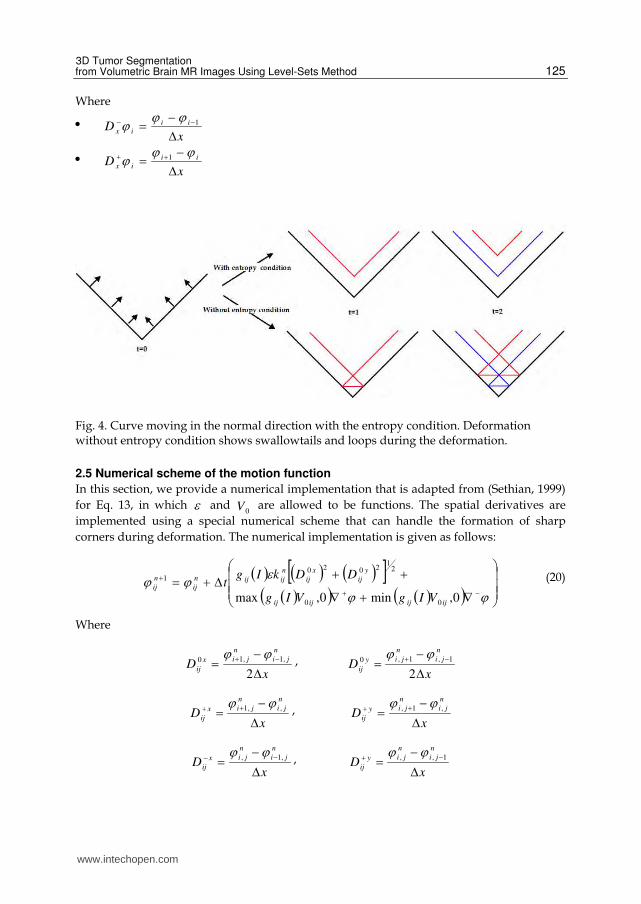
loops formation during the deformation. Once the corner is developed, it is not clear how to continue the deformation, since the definition of the normal direction becomes ambiguous (Fig. 4.). A natural way to continue the deformation is to impose the so-called entropy condition originally proposed in the area of interface propagation by Sethian (Sethian, 1982), (Sethian, 1994). Since the numerical scheme of the spatial gradient in one space dimension can be written as follows:

x

ii

i

2

11 (18)

When, there is a deformation in various directions, (wheni is the curvature k factor);

21

22

0,min0,max xixi DD (19)

When, there is a constant deformation, (when i is constant deformation

0V factor);

www.intechopen.com


125

Where

x

D ii

ix 1

x

D ii

ix 1

Fig. 4. Curve moving in the normal direction with the entropy condition. Deformation without entropy condition shows swallowtails and loops during the deformation.

2.5 Numerical scheme of the motion function

In this section, we provide a numerical implementation that is adapted from (Sethian, 1999)

for Eq. 13, in which and 0V are allowed to be functions. The spatial derivatives are

implemented using a special numerical scheme that can handle the formation of sharp

corners during deformation. The numerical implementation is given as follows:

0,min0,max 00

21

20201

ijijijij

y

ij

x

ij

n

ijijn

ij

n

ij

VIgVIg

DDkIgt (20)

Where

xD

n

ji

n

jix

ij

2

,1,10

, x

D

n

ji

n

jiy

ij

2

1,1,0

xD

n

ji

n

jix

ij ,,1

, x

D

n

ji

n

jiy

ij ,1,

xD

n

ji

n

jix

ij ,1,

, x

D

n

ji

n

jiy

ij 1,,

www.intechopen.com


126

2

1

22

22

)0,min()0,max(

)0,min()0,max(

ij

y

ijij

y

ij

ij

x

ijij

x

ij

DD

DD

2

1

22

22

)0,max()0,min(

)0,max()0,min(

ij

y

ijij

y

ij

ij

x

ijij

x

ij

DD

DD

As it has been specified previously, the level-Sets function evolves using a speed function for the zero level-Sets only and using extended speed functions. Accordingly, the level-Sets can lose its property of being a signed distance function, causing inaccuracy in curvature and normal calculations. As a result, re-initialization of the level-Sets function to a signed distance function is often required for these schemes. Usually, the distance map is reset using the following equation (Sussman & al., 1997):

1signet

(21)

Where

11

11

11

si

si

si

signe

Since the curve or the surface of ROI is recovred from the zero level-Sets only. We must therefore detect the zero values of the function .We can only detect differences in sign between two consecutive points in either direction, horizontal and vertical. The detection of points jiP , of zero level-Sets by Malladi (Malladi & al., 1995) is done according to the following algorithm: Recovering interface algorithm:

Function isfront

ji,

if 01,1,1,,,1,,max jijijiji

and

01,1,1,,,1,,min jijijiji

or

0,max ji

then

tjiP ,

else

tjiP , end end

www.intechopen.com


127

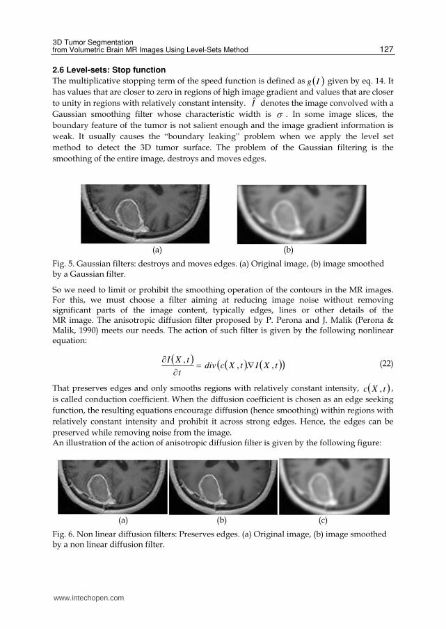
2.6 Level-sets: Stop function

The multiplicative stopping term of the speed function is defined as Ig given by eq. 14. It

has values that are closer to zero in regions of high image gradient and values that are closer

to unity in regions with relatively constant intensity. I denotes the image convolved with a

Gaussian smoothing filter whose characteristic width is . In some image slices, the

boundary feature of the tumor is not salient enough and the image gradient information is

weak. It usually causes the “boundary leaking” problem when we apply the level set

method to detect the 3D tumor surface. The problem of the Gaussian filtering is the

smoothing of the entire image, destroys and moves edges.

(a) (b)

Fig. 5. Gaussian filters: destroys and moves edges. (a) Original image, (b) image smoothed by a Gaussian filter.

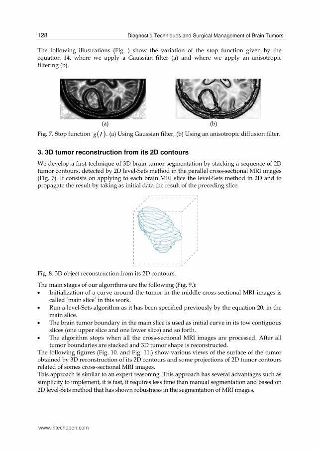
So we need to limit or prohibit the smoothing operation of the contours in the MR images. For this, we must choose a filter aiming at reducing image noise without removing significant parts of the image content, typically edges, lines or other details of the MR image. The anisotropic diffusion filter proposed by P. Perona and J. Malik (Perona & Malik, 1990) meets our needs. The action of such filter is given by the following nonlinear equation:

tXItXcdivt

tXI,.,

, (22)

That preserves edges and only smooths regions with relatively constant intensity, tXc , ,

is called conduction coefficient. When the diffusion coefficient is chosen as an edge seeking

function, the resulting equations encourage diffusion (hence smoothing) within regions with

relatively constant intensity and prohibit it across strong edges. Hence, the edges can be

preserved while removing noise from the image. An illustration of the action of anisotropic diffusion filter is given by the following figure:

(a) (b) (c)

Fig. 6. Non linear diffusion filters: Preserves edges. (a) Original image, (b) image smoothed by a non linear diffusion filter.

www.intechopen.com


128

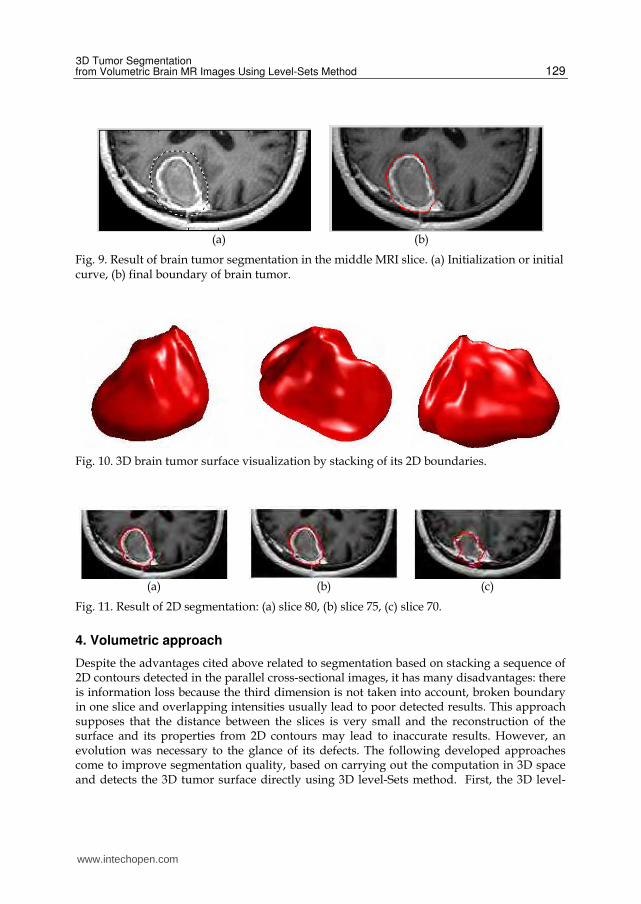
The following illustrations (Fig. ) show the variation of the stop function given by the equation 14, where we apply a Gaussian filter (a) and where we apply an anisotropic filtering (b).

(a) (b)

Fig. 7. Stop function Ig . (a) Using Gaussian filter, (b) Using an anisotropic diffusion filter.

3. 3D tumor reconstruction from its 2D contours

We develop a first technique of 3D brain tumor segmentation by stacking a sequence of 2D tumor contours, detected by 2D level-Sets method in the parallel cross-sectional MRI images (Fig. 7). It consists on applying to each brain MRI slice the level-Sets method in 2D and to propagate the result by taking as initial data the result of the preceding slice.

Fig. 8. 3D object reconstruction from its 2D contours.

The main stages of our algorithms are the following (Fig. 9.):

Initialization of a curve around the tumor in the middle cross-sectional MRI images is called ‘main slice’ in this work.

Run a level-Sets algorithm as it has been specified previously by the equation 20, in the main slice.

The brain tumor boundary in the main slice is used as initial curve in its tow contiguous slices (one upper slice and one lower slice) and so forth.

The algorithm stops when all the cross-sectional MRI images are processed. After all tumor boundaries are stacked and 3D tumor shape is reconstructed.

The following figures (Fig. 10. and Fig. 11.) show various views of the surface of the tumor obtained by 3D reconstruction of its 2D contours and some projections of 2D tumor contours related of somes cross-sectional MRI images. This approach is similar to an expert reasoning. This approach has several advantages such as

simplicity to implement, it is fast, it requires less time than manual segmentation and based on

2D level-Sets method that has shown robustness in the segmentation of MRI images.

www.intechopen.com


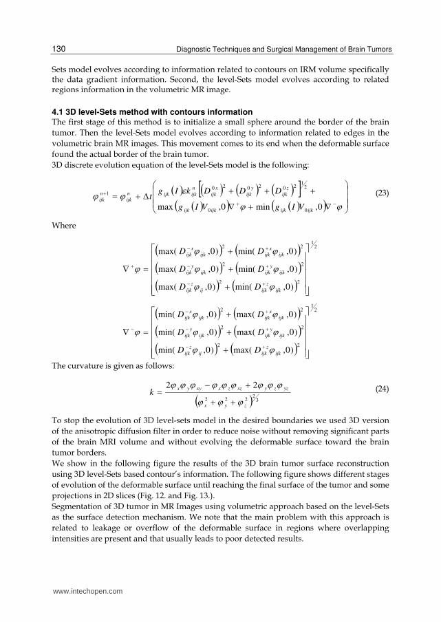
129

(a) (b)

Fig. 9. Result of brain tumor segmentation in the middle MRI slice. (a) Initialization or initial curve, (b) final boundary of brain tumor.

Fig. 10. 3D brain tumor surface visualization by stacking of its 2D boundaries.

(a) (b) (c)

Fig. 11. Result of 2D segmentation: (a) slice 80, (b) slice 75, (c) slice 70.

4. Volumetric approach

Despite the advantages cited above related to segmentation based on stacking a sequence of 2D contours detected in the parallel cross-sectional images, it has many disadvantages: there is information loss because the third dimension is not taken into account, broken boundary in one slice and overlapping intensities usually lead to poor detected results. This approach supposes that the distance between the slices is very small and the reconstruction of the surface and its properties from 2D contours may lead to inaccurate results. However, an evolution was necessary to the glance of its defects. The following developed approaches come to improve segmentation quality, based on carrying out the computation in 3D space and detects the 3D tumor surface directly using 3D level-Sets method. First, the 3D level-

www.intechopen.com


130

Sets model evolves according to information related to contours on IRM volume specifically the data gradient information. Second, the level-Sets model evolves according to related regions information in the volumetric MR image.

4.1 3D level-Sets method with contours information The first stage of this method is to initialize a small sphere around the border of the brain

tumor. Then the level-Sets model evolves according to information related to edges in the

volumetric brain MR images. This movement comes to its end when the deformable surface

found the actual border of the brain tumor.

3D discrete evolution equation of the level-Sets model is the following:

0,min0,max 00

21

2020201

ijkijkijkijk

z

ijk

y

ijk

x

ijk

n

ijkijkn

ijk

n

ijk

VIgVIg

DDDkIgt (23)

Where

2

1

22

22

22

)0,min()0,max(

)0,min()0,max(

)0,min()0,max(

ijk

z

ijkij

z

ijk

ijk

y

ijkijk

y

ijk

ijk

x

ijkijk

x

ijk

DD

DD

DD

2

1

22

22

22

)0,max()0,min(

)0,max()0,min(

)0,max()0,min(

ijk

z

ijkij

z

ijk

ijk

y

ijkijk

y

ijk

ijk

x

ijkijk

x

ijk

DD

DD

DD

The curvature is given as follows:

32

222

22

zyx

yzzyxzzxxyyxk

(24)

To stop the evolution of 3D level-sets model in the desired boundaries we used 3D version

of the anisotropic diffusion filter in order to reduce noise without removing significant parts

of the brain MRI volume and without evolving the deformable surface toward the brain

tumor borders.

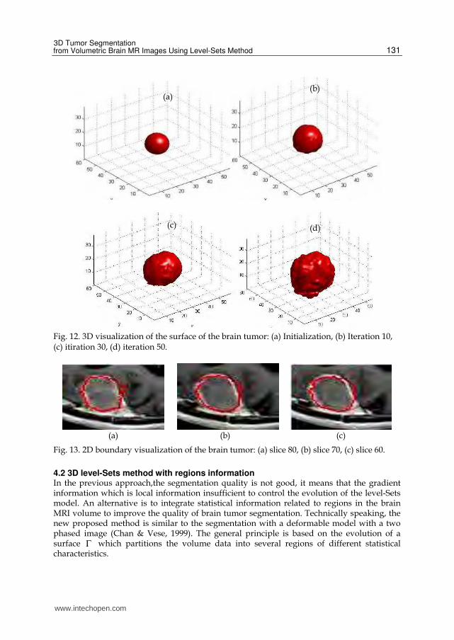
We show in the following figure the results of the 3D brain tumor surface reconstruction

using 3D level-Sets based contour’s information. The following figure shows different stages

of evolution of the deformable surface until reaching the final surface of the tumor and some

projections in 2D slices (Fig. 12. and Fig. 13.).

Segmentation of 3D tumor in MR Images using volumetric approach based on the level-Sets

as the surface detection mechanism. We note that the main problem with this approach is

related to leakage or overflow of the deformable surface in regions where overlapping

intensities are present and that usually leads to poor detected results.

www.intechopen.com


131

Fig. 12. 3D visualization of the surface of the brain tumor: (a) Initialization, (b) Iteration 10, (c) itiration 30, (d) iteration 50.

(a) (b) (c)

Fig. 13. 2D boundary visualization of the brain tumor: (a) slice 80, (b) slice 70, (c) slice 60.

4.2 3D level-Sets method with regions information In the previous approach,the segmentation quality is not good, it means that the gradient information which is local information insufficient to control the evolution of the level-Sets model. An alternative is to integrate statistical information related to regions in the brain MRI volume to improve the quality of brain tumor segmentation. Technically speaking, the new proposed method is similar to the segmentation with a deformable model with a two phased image (Chan & Vese, 1999). The general principle is based on the evolution of a surface which partitions the volume data into several regions of different statistical characteristics.

(a)(b)

(c) (d)

www.intechopen.com


132

A single deformable surface allows segmentation into two regions in and

out , where

in represents the region that circumscribed by the surface and out the outer region

(Angelini, 2005). The information that controls the evolution of the the new level-Sets model is usually based on statistical modelling of the various region in the volumetric data.

We assume that the image zyxI ,, defined on the domain is composed of two

homogeneous regions of distinct values 0I and

1I and that the tumor region to detect

corresponds to the region of intensity0I . We denote the boundary of the tumor with

intensity 0I by . For a given surface of the domain , we consider the following

energy functional E :

outin

dcIdcIALE2

110

2

000 (25)

Where 1c and

2c are equal respectively to the average value of inside and outside of the

surface . L and A are the regularizing terms corresponding respectively to the

length of the curve and the area of the object enclosed by the curve.

21 ,,, are fixed positive parameters.

Segmentation of the brain tumor from volumetric MRI image is performed via minimization

of the energy functional defined in Eq. (26). Minimization of the functional is proceeded

using a steepest gradient descent on a discrete spatial grid indexed with 3,, kji and

introduction of a temporal index (n) leads to an iterative scheme with the following equation

of the level-Sets evolution model:

2

22

2

11

1 n

ijkijk

n

ijkijk

n

ijk

n

ijk

n

ijk

n

ijk cIcIkt (26)

To segment the brain tumor using this approach (Fig. 14.), we initialized an initial surface

through its boundary. Then this surface evolves until reaching the actual border of the tumor.

Several criteria can be incorporated to stop the process of segmentation: when the area of the

deformable surface becomes constant or the volume of the region bounded by the deformable

surface becomes constant or Energy function E reaches its minimum value. The latter

criterion is sufficient but it has a problem of computational cost. The convergence of the

deformable surface to the tumor border implies that the area and the volume of deformable

surface becomes constant. However, area and volume computational is less. For this, we used

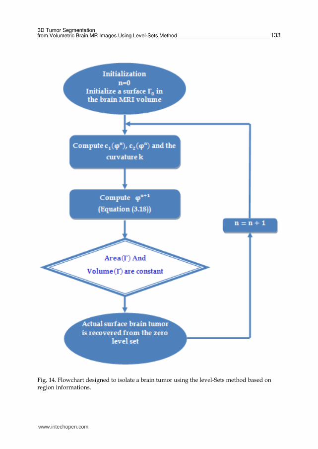
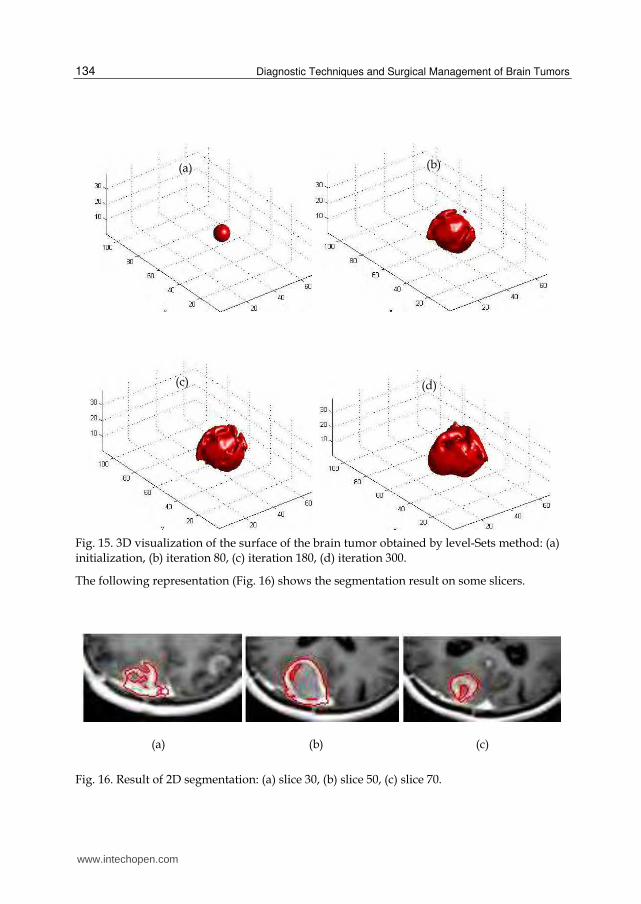
as a stopping condition, area and volume of the deformable surface at a time. We present above a flowchart designed in our research to isolate a brain tumor using level-Sets method based on region informations: This method consists in initializing a small sphere through the border of the brain tumor. Then the level-Sets model evolves according to related region information in the image in order to plate itself on the surface of the tumor. We show in the following the results of the 3D reconstruction of the brain tumor surface relayed to this approach. The following figure shows different stages of evolution of the deformable surface until reaching the final surface of the tumor and some projections in 2D slices (Fig. 15. and Fig. 16.). These results show that this approach combine the following advantages: arbitrary initialization of the object anywhere in the image, no need for gradient information, self adaptation for inward and outward local motion.

www.intechopen.com


133

Fig. 14. Flowchart designed to isolate a brain tumor using the level-Sets method based on region informations.

www.intechopen.com


134

Fig. 15. 3D visualization of the surface of the brain tumor obtained by level-Sets method: (a) initialization, (b) iteration 80, (c) iteration 180, (d) iteration 300.

The following representation (Fig. 16) shows the segmentation result on some slicers.

(a) (b) (c)

Fig. 16. Result of 2D segmentation: (a) slice 30, (b) slice 50, (c) slice 70.

(a) (b)

(c) (d)

www.intechopen.com


135

5. Summary and discussion

Presented research was provided with a general goal to develop 3D segmentation

algorithms of brain tumor from volumetric MRI images. We have presented a variational

method, 3D level-Sets applied to automatic segmentation of brain tumor in MRIs, using

boundary and region based information of tumor to control the deformable surface

propagation. The first approach used, is the 3D reconstruction from its 2D contours using a

sequence of 2D contours, detected by 2D level-Sets method in the parallel cross-sectional

MRI images. This method goes very well but it has two major defects, there is no interaction

between the slices and surface must be cylindrical. This approach is the most simple that

one can make. It makes it possible to use active contours in the field 2D method which

showed its robustness. However, an evolution was necessary to the glance of its defects

related to the results obtained and the tumor shapes that were being able to be treated. The

second approach comes to improve the segmentation quality, based on carrying out the

computation in 3D space and detecting the brain tumor region directly using 3D level-Sets

method. In the first volumetric approach 3D level-Sets model evolves according to

information related to contours on IRM volume. In the second level -Sets model evolves

according to related regions descriptors in the volumetric MR image. Evaluations were

performed on a set of volumetric MRI images obtained from (MeDEISA) database.

6. References

Kass, M.; Witkin, A. & Terzopoulos, D. (1988). Snakes: Active contour models. International

Journal of Computer Vision V. 1, no. , pp. 321-331, 1988.

Terzopoulos, D.; Witkin, A.; & Kass, M. (1988). Constraints on deformable models:

Recovering 3D shape and nonrigid motion. Artificial Intelligence, vol. 36, pp. 91. -1

23.1988.

Amini, A.; Weymouth, T.; & Jain, R. (1990). Using dynamic programming for solving

variational problems in vision. IEEE Trans. Patt. Anal. Mach. Intell., vol. 12, no. 9,

pp. 855–867, 1990.

Cohen, L. (1991). On active contour models and balloons. CVGIP: Imag. Under., vol. 53, no.

2, pp. 211–218, 1991.

McInerney, T. & Terzopoulos, D. (1995). A dynamic finite element surface model for

segmentation and tracking in multidimensional medical images with application to

cardiac 4D image analysis. Comp. Med. Imag. Graph., vol. 19, no. 1, pp. 69–83,

1995.

Caselles, V.; Catte, F.; Coll, T. & Dibos, F. (1993). A geometric model for active contours.

Numerische Mathematik, vol. 66, pp. 1–31, 1993.

Malladi, R.; Sethian, J. & Vemuri, B. (1995). Shape modeling with front propagation: A

level set approach,” IEEE Trans. Patt. Anal. Mach. Intell., vol. 17, no. 2, pp. 158–

175, 1995.

Caselles, V.; Kimmel, R. & Sapiro, G. (1995). Geodesic active contours. 5th International

Conf. Comp. Vis., pp. 694–699, 1995.

www.intechopen.com


136

Whitaker, R. (1994). Volumetric deformable models: active blobs. Tech. Rep.

ECRC-94-25, European Computer-Industry Research Centre GmbH,

1994.

Sapiro, G. & Tannenbaum, A. (1993). Affine invariant scale-space,” International Journal

Computer Vision, vol. 11, no. 1, pp. 25–44, 1993.

Kimia, B.; Tannenbaum, A. & Zucker, S. (1995). Shapes, shocks, and deformations: the

components of two-dimensional shape and the reaction-diffusion space.

International Journal Computer Vision. vol. 15, pp. 189–224, 1995.

Kimmel, R.; Amir, A. & Bruckstein, M. (1995). Finding shortest paths on surfaces using level

sets propagation. IEEE Trans. Patt. Anal. Mach. Intell., vol. 17, no. 6, pp. 635–640,

1995.

Alvarez, L.; Guichard, F.; Lions, P. & Morel, J. (1993). Axioms and fundamental equations of

image processing,” Archive for Rational Mechanics and Analysis, vol. 123, no. 3,

pp. 199–257, 1993.

Osher, S. & Sethian, J. (1988). Fronts propagating with curvature-dependent speed:

algorithms based on Hamilton-Jacobi formulations. J. Computational Physics, vol.

79, pp. 12–49, 1988.

Sethian, J. (1999). Level Set Methods and Fast Marching Methods: Evolving

Interfaces in Computational Geometry, Fluid Mechanics. Computer Vision,

and Material Science. Cambridge, UK: Cambridge University Press, 2nd ed.,

1999.

Kimia, B. (1990). Conservation Laws and a Theory of Shape. Ph.D. thesis, McGill Centre for

Intelligent Machines, McGill University, Montreal, Canada, 1990.

Grayson, M. (1985). Shortening embedded curves. Annals of Mathematics, vol. 129, pp. 71–

111, 1989.

Sethian, J. (1985). Curvature and evolution of fronts. Commun. Math. Phys., vol. 101, pp.

487–499, 1985.

Sethian, J. (1989). A review of recent numerical algorithms for hypersurfaces moving

with curvature dependent speed. J. Differential Geometry, vol. 31, pp. 131–161,

1989.

Williams, D. & Shah, M. (1992). A fast algorithm for active contours and curvature

estimation. CVGIP: Imag. Under., vol. 55, no. 1, pp. 14–26, 1992.

Malladi, R., Sethian, J. & Vemuri, C. (1995). Shape Modeling with Front Propagation: A

Level Set Approach, IEEE Trans. on Pattern Analysis and Machine Intelligence, 17,

2, pp. 158–175, 1995.

Sethian, J. (1982). An Analysis of Flame Propagation. Ph.D. thesis, Dept. of Mathematics,

University of California, Berkeley, CA, 1982.

Sethian, J. (1994). Curvature flow and entropy conditions applied to grid

generation.

Journal of Computational Physics, 115 : 440−454, 1994.

Sussman, M.; Fatemi, E.; Smereka, P. & Osher, S. (1997). An improved level set method for

incompressible two-phase flows. Computers and Fluids, vol. 27, 5-6, pp. 663-680,

1997.

www.intechopen.com


137

Perona, P. & Malik, J. (1990). Scale-space and edge detection using anisotropic diffusion.

IEEE Trans. Pattern Anal. Machine Intell., 12 :629.639, 1990.

Chan, T. & Vese, L. (1999). An Active Contour model without Edges. In LNCS, edited by M.

Neilsen, P. Johanson, O.F. Olson and J. Weickert, Springer-Verlag, Berlin/New

York. Vol. 1687, 141-151,1999.

Angelini, E. (2005). Segmentation of Real-Time Three-Dimensional Ultrasound

for Quantification of Ventricular Function: A Clinical Study on Right and

Left Ventricles, Ultrasound in Med. & Biol., Vol. 31, No. 9, pp. 1143–1158,

2005.

Sahoo, K.; Soltani, S.; Wong, C. & Chen, Y. (1988). A survey of thresholding techniques.

Computer Vision Graphics Image Processing 1988; 41: pp233 – 260.

Moon, N.; Bulitt, E.; Leemput, K. and Gerig, G (2002). Model-based brain and tumor

segmentation. Proceedings of ICPR 2002; 1: 528-531.

Wang, Z.; Hu, Q.; Loe, K.; Aziz, A. & Nowinski, L. (2004) Rapid and Automatic

Detection of Brain Tumors in MR Images. Proceeding of SPIE 2004; 5369: 602 –

612.

Michael, K.; Simon, W.; Arya, N.; Peter, B.; Ferenc, J. & Ron, K. (2001)

Automated Segmentation of MR Images of Brain Tumors. Radiology 2001; 218:

586 – 591.

Taheri, S.; Ong, S. & Chong, V. (2009). Level-set Segmentation of Brain Tumors using a

Threshold-based Speed Function," Image and Vision Computing (IVC) Elsevier

Journal, 2009.

Taheri, S.; Ong, S. & Chong, V. (2007). Threshold-based 3D Tumor Segmentation using Level

Set (TSL). In Proc. IEEE Workshop on Application of Computer Vision (WACV),

2007.

Lefohn, A.; Cates, J. & Whitaker, R. (2003). Interactive, GPU- Based Level Sets for 3D Brain

Tumor Segmentation, MICCAI 2003.

Lynn, F.; Lawrence, H.; Dmitry, G. & Murtagh, R. (2001). Automatic segmentation of non-

enhancing brain tumors in magnetic resonance images. Artificial Intelligence in

Medicine 2001; 21(1-3): pp 43 – 63.

MeDEISA, (2010). Medical Database for the Evaluation of Image and Signal processing

(MeDEISA), http://www.medeisa.net.

Lima, P.; Bonarini, A. & Mataric, M. (2004). Application of Machine Learning, InTech, ISBN

978-953-7619-34-3, Vienna, Austria

Li, B.; Xu, Y. & Choi, J. (1996). Applying Machine Learning Techniques, Proceedings of ASME

2010 4th International Conference on Energy Sustainability, pp. 14-17, ISBN 842-6508-

23-3, Phoenix, Arizona, USA, May 17-22, 2010

Siegwart, R. (2001). Indirect Manipulation of a Sphere on a Flat Disk Using Force

Information. International Journal of Advanced Robotic Systems, Vol.6, No.4,

(December 2009), pp. 12-16, ISSN 1729-8806

Arai, T. & Kragic, D. (1999). Variability of Wind and Wind Power, In: Wind Power, S.M.

Muyeen, (Ed.), 289-321, Scyio, ISBN 978-953-7619-81-7, Vukovar, Croatia

Van der Linden, S. (June 2010). Integrating Wind Turbine Generators (WTG’s) with

Energy Storage, In: Wind Power, 17.06.2010, Available from

www.intechopen.com


138

http://sciyo.com/articles/show/title/wind-power-integrating-wind-turbine-

generators-wtg-s-with-energy-storage

www.intechopen.com

Diagnostic Techniques and Surgical Management of Brain TumorsEdited by Dr. Ana Lucia Abujamra

ISBN 978-953-307-589-1Hard cover, 544 pagesPublisher InTechPublished online 22, September, 2011Published in print edition September, 2011

InTech EuropeUniversity Campus STeP Ri Slavka Krautzeka 83/A 51000 Rijeka, Croatia Phone: +385 (51) 770 447 Fax: +385 (51) 686 166www.intechopen.com

InTech ChinaUnit 405, Office Block, Hotel Equatorial Shanghai No.65, Yan An Road (West), Shanghai, 200040, China

Phone: +86-21-62489820 Fax: +86-21-62489821

The focus of the book Diagnostic Techniques and Surgical Management of Brain Tumors is on describing theestablished and newly-arising techniques to diagnose central nervous system tumors, with a special focus onneuroimaging, followed by a discussion on the neurosurgical guidelines and techniques to manage and treatthis disease. Each chapter in the Diagnostic Techniques and Surgical Management of Brain Tumors isauthored by international experts with extensive experience in the areas covered.

How to referenceIn order to correctly reference this scholarly work, feel free to copy and paste the following:

Kamel Aloui and Mohamed Saber Naceur (2011). 3D Tumor Segmentation from Volumetric Brain MR ImagesUsing Level-Sets Method, Diagnostic Techniques and Surgical Management of Brain Tumors, Dr. Ana LuciaAbujamra (Ed.), ISBN: 978-953-307-589-1, InTech, Available from:http://www.intechopen.com/books/diagnostic-techniques-and-surgical-management-of-brain-tumors/3d-tumor-segmentation-from-volumetric-brain-mr-images-using-level-sets-method

© 2011 The Author(s). Licensee IntechOpen. This chapter is distributedunder the terms of the Creative Commons Attribution-NonCommercial-ShareAlike-3.0 License, which permits use, distribution and reproduction fornon-commercial purposes, provided the original is properly cited andderivative works building on this content are distributed under the samelicense.

https://creativecommons.org/licenses/by-nc-sa/3.0/

Documents

3D Tumor Segmentation from Volumetric Brain MR Images ...cdn.intechweb.org/pdfs/20267.pdf · 3D Tumor Segmentation from Volumetric Brain ... of neuro-imaging, ... 3D Tumor Segmentation