Embed Size (px)
Citation preview

This content has been downloaded from IOPscience. Please scroll down to see the full text.
Download details:
IP Address: 194.177.201.132
This content was downloaded on 13/06/2014 at 07:12
Please note that terms and conditions apply.
3D stability analysis of Rayleigh–Bénard convection of a liquid metal layer in the presence of a
magnetic field—effect of wall electrical conductivity
View the table of contents for this issue, or go to the journal homepage for more
2014 Fluid Dyn. Res. 46 055507
(http://iopscience.iop.org/1873-7005/46/5/055507)
Home Search Collections Journals About Contact us My IOPscience
3D stability analysis of Rayleigh–Bénardconvection of a liquid metal layer in thepresence of a magnetic field—effect of wallelectrical conductivity
Dimitrios Dimopoulos and Nikos A Pelekasis
Department of Mechanical & Industrial Engineering, University of Thessaly, PedionAreos, Volos 38334, Greece
E-mail: [email protected]
Received 2 July 2013, revised 2 April 2014Accepted for publication 7 May 2014Published 12 June 2014
Communicated by A D Gilbert
AbstractRayleigh–Bénard stability of a liquid metal layer of rectangular cross section isexamined in the presence of a strong magnetic field that is aligned with thehorizontal direction of the cross section. The latter is much longer than thevertical direction and the cross section assumes a large aspect ratio. The sidewalls are treated as highly conducting. Linear stability analysis is performedallowing for three-dimensional instabilities that develop along the longitudinaldirection. The finite element methodology is employed for the discretization ofthe stability analysis formulation while accounting for the electrical con-ductivity of the cavity walls. The Arnoldi method provides the dominanteigenvalues and eigenvectors of the problem. In order to facilitate parallelimplementation of the numerical solution at large Hartmann numbers, Ha,domain decomposition is employed along the horizontal direction of the crosssection. As the Hartmann number increases a real eigenvalue emerges as thedominant unstable eigenmode, signifying the onset of thermal convection,whose major vorticity component in the core of the layer is aligned with thedirection of the magnetic field. Its wavelength along the longitudinal directionof the layer is on the order of twice its height and increases as Ha increases.The critical Grashof was obtained for large Ha and it was seen to scale likeHa2 signifying the balance between buoyancy and Lorentz forces. For wellconducting side walls, the nature of the emerging flow pattern is determinedby the combined conductivity of Hartmann walls and Hartmann layers,cH+Ha
−1. When poor conducting Hartmann walls are considered, cH≪ 1, thecritical eigensolution is characterized by well defined Hartmann and side
0169-5983/14/055507+31$33.00 © 2014 The Japan Society of Fluid Mechanics and IOP Publishing Ltd Printed in the UK 1
| The Japan Society of Fluid Mechanics Fluid Dynamics Research
Fluid Dyn. Res. 46 (2014) 055507 (31pp) doi:10.1088/0169-5983/46/5/055507
layers. The side layers are characterized by fast fluid motion in the magneticfield direction as a result of the electromagnetic pumping in the vicinity of theHartmann walls. Increasing the electrical conductivity of the Hartmann wallswas seen to delay the onset of thermal convection, while retaining the abovescaling at criticality. Furthermore, for both conducting and insulating Hart-mann walls and the entire range of Ha numbers that was examined, there wasno tendency for a well defined quasi two-dimensional structure to developowing to the convective motion in the core. A connection is made between theabove findings and previous experimental investigations indicating the onsetof standing waves followed by travelling waves as Gr is further increasedbeyond its critical value.
1. Introduction
It is a well established fact that a magnetic field tends to eliminate the vorticity componentsthat are perpendicular to it while leaving almost unaffected those that are aligned with it(Chandrasekhar 1961, Sommeria and Moreau 1982). As a result, upon increasing the intensityof the magnetic field variations along its direction are suppressed and quasi two-dimensionalstructures emerge. As a concomitant effect of increasing the magnetic field intensity, thinvortical layers develop near channel walls that are aligned or perpendicular to the magneticfield. The latter are called Hartmann layers and are determined by the balance betweenviscous and Lorentz forces whereas the former are called side layers and are characterized bythe balance between pressure and viscous forces (Buhler 1996, 1998). Such structures havebeen reported in the literature of experimental magnetohydrodynamics both in the context offorced and free convection flows (Potherat et al 2000, 2005). Furthermore, such quasi two-dimensional structures persist in the turbulent flow regime and are considered as an inter-mediate state on the path towards three-dimensional turbulence as Reynolds/Grashofincreases in forced/free convection flows for fixed large Hartmann numbers, in the mannerproposed by Sommeria and Moreau (1982).
In the context of Rayleigh–Bénard convection the flow arrangement in a rectangular box,that was heated from below in the presence of a strong magnetic field, was studied by Burrand Muller 2002 (referred to henceforth as BM for brevity). The onset of steady convectionwas registered as a function of Hartmann, Ha, as the heat flux and consequently the Grashofnumber was increased. Over a wide range of Hartmann numbers, 100 < Ha < 1000, pre-ferential arrangement of the emerging recirculation rolls in the direction of the magnetic fieldwas observed by monitoring the horizontal anisotropy coefficient. As Grashof increasedbeyond the threshold for stationary convection the onset of time dependent convection wascaptured that characterizes the flow pattern in the large Grashof or intermediate Hartmannregime. In fact, a maximum in the heat transfer rate was registered along the vertical directionin the parameter range corresponding to transient convection, that was attributed to the quasitwo-dimensional arrangement of the recirculation rolls in the box. When the magnetic field isnot strong enough to suppress fluctuations of the velocity and temperature fields but largeenough to eliminate vortices that are not aligned with it, the intensity of fluctuation of thedominant remaining vortex increases the amount of heat convected from the bottom towardsthe top wall thus generating conditions for optimal heat transfer. This is an interestingdynamical aspect of the flow arrangement in the presence of a magnetic field that may lead touseful intensification of heat or mass transfer by controlling the orientation and intensity ofthe generated recirculation rolls. The threshold for the onset of thermal convection was
Fluid Dyn. Res. 46 (2014) 055507 D Dimopoulos and N A Pelekasis
2
obtained in the aforementioned study by employing the quasi 2d assumption for the emergingflow pattern. Finally, it should also be pointed out that turbulent fluctuations were reported atlarge Hatmann numbers in a range of Grashof numbers for which a large degree of non-isotropy was registered in the horizontal plane, thus indicating the onset of quasi 2dturbulence.
The stabilizing effect of the magnetic field is a recurring theme in studies of free con-vection flows. Its effect on the onset of standing and traveling wave instabilities has beenaddressed in various contexts including its importance, as Hartman increases, in establishingquasi 2D transient or turbulent flow structures. Transition from standing to traveling waveconvection patterns in the 2D stability of a vertical layer of electrically conducting fluid inelectrically insulating walls, was studied by Takashima (1994) for a wide range of Prandtl andGrashof numbers at selected Hartmann values, capturing the stabilizing effect of the trans-verse magnetic field. Three dimensional stability of buoyant flow in a horizontal channel withelectrically insulating walls was studied by Lyubimov et al (2009), subject to a longitudinaltemperature gradient and vertical or transverse magnetic field. A standing wave mode wasidentified as the dominant instability and the stabilizing effect of the magnetic field wasverified, especially as the width of the cross section was increased. The formation of Hart-mann and side layers was also ascertained with increasing Hartmann number for the case of ahorizontal magnetic field, whereas jet formation was registered at steady conditions when avertical magnetic field was applied. More recently, the quasi 2D assumption has beenemployed in order to study the stability of free and mixed convection flows at large Hartmannvalues. Gelfgat and Molokov (2011) studied the stability of recirculation vortices when themagnetic field is perpendicular to the plane of circulation using the quasi 2D flow assumption,and showed the dependence of the stability pattern on the box aspect ratio and boundaryconditions. Smolentsev et al (2012) studied the stability of the M-shaped profile in an upwardflow in order to assess the relative importance of jet formation and the appearance ofinflection points in the base flow velocity profile, in destabilizing the flow. In a subsequentstudy Vetcha et al (2013) examined the stability of upward mixed convection flow via thequasi 2d assumption and three-dimensional direct numerical simulations, in an effort tosimulate flow arrangement in the poloidal ducts of the so called dual-coolant lead–lithium(DCLL) blanket, with satisfactory agreement; Smolentsev et al (2008).
As is evident from the above, the above ideas are useful in understanding the dynamicphenomena that take place in ducts that carry liquid metals, as is the case in fusion reactorblankets. The latter are designed so that they consist of modules where liquid metal iscirculated inside ducts, under the influence of the magnetic field generated in the plasmareactor. In the DCLL blanket concept (Buhler and Norajitra 2003, Smolentsev et al 2008) aliquid lead–lithium alloy is used for assisting heat transfer, along with separate heliumcooling, besides breeding tritium. In this case forced convection dominates in the duct crosssection and SiC inserts are employed in order to electrically insulate the side walls andconsequently mitigate the intensity of jets that are generated near the side walls when theirconductivity is very high. Such high speed jets curry most of the liquid metal in the duct andgenerate instabilities, Smolentsev et al (2012) and Vetcha et al (2013), that result in increasedmixing and excessive heating of the side walls.
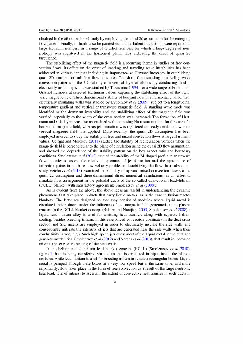
In the helium-cooled lithium–lead blanket concept (HCLL) (Smolentsev et al 2010),figure 1, heat is being transferred via helium that is circulated in pipes inside the blanketmodules, while lead–lithium is used for breeding tritium in separate rectangular boxes. Liquidmetal is pumped through these boxes at a very low speed but at the same time, and moreimportantly, flow takes place in the form of free convection as a result of the large neutronicheat load. It is of interest to ascertain the extent of convective heat transfer in such ducts in
Fluid Dyn. Res. 46 (2014) 055507 D Dimopoulos and N A Pelekasis
3
order to properly predict the combined heat transfer coefficient of a module consisting ofpipes carrying helium and ducts where liquid metal is circulated. Such predictions areessential for assessing the heat load on the metallic walls of the pipes and cavities andconsequently estimating their life cycle.
In this context the 3D stability of a liquid metal layer that rests in a box of rectangularcross section, subject to a large magnetic field and exposed to a thermal gradient that isopposite to the direction of gravity, is very important in establishing the flow pattern in thebox as well as the mode by which heat is being transferred. Based on estimates of theparameters pertaining to the operation of the liquid metal carrying/breeding boxes that areemployed in the HCLL blanket, the Hartmann (Ha) and Grashof (Gr) numbers will be in therange of 20 000 and 5 × 10⁹, respectively. The large value of Gr is a result of the intenseneutronic heat load that is anticipated to arise in large fusion reactors like ITER (Buhler andNorajitra 2003, Kharitsa et al 2004, Smolentsev et al 2010). Early attempts to model the flowconditions in the blanket boxes where liquid metal is circulated (Kharitsa et al 2004; BM)assume a quasi two-dimensional flow arrangement in the cavity with well established Hart-mann and side walls. This approximation is based on asymptotic estimates for the scaling ofinertia in buoyant magnetohydrodynamic convection in ducts (Buhler 1998), i.e. inertia isneglected as long as Gr≪Ha5/2, with well defined Hartmann and side layers. Substituting theabove estimates for fusion reactors Gr/Ha5/2∼ 0.5. Therefore it is of interest to establish thescaling for the onset of convective effects in such cavities. The experimental study reportedby BM is an attempt in this direction where instead of a volumetric heat load the temperaturegradient that sets the Grashof number is established via a constant heat flux that is applied atthe bottom horizontal wall.
Fluid Dyn. Res. 46 (2014) 055507 D Dimopoulos and N A Pelekasis
4
Figure 1. Schematic diagram of a blanket module pertaining to the HCLL designconcept (adapted from the study by Buhler and Mistrangelo (2010)).
As was stressed above, the electrical conductivity of the walls is expected to play animportant role in the dynamics and heat transfer of this flow arrangement. The present studyaims at addressing this particular issue by identifying the structure of the dominant eigen-solution for free convection dominated flow in one box, along with the scaling of the criticalGrashof number, GrCr, as a function of Ha and electrical wall conductivities, in the context oflinear stability analysis. In particular, the validity of the hypothesis that the emerging steadyconvection pattern assumes a quasi 2D structure with well defined Hartmann and side layerswill be examined as the electrical conductivity of the Hartmann walls varies. Flow is assumedto take place only as a result of free convection while periodicity is assumed in the directionperpendicular to the plane defined by the magnetic field and gravitational acceleration.
In the next section, the full problem formulation is presented as well as the linearizedform allowing for three dimensional disturbances. In section 3 the finite element formulationfor the stability problem is presented. Emphasis is placed on the discretization of the equationgoverning variations of the electric potential and the inclusion of the boundary conditions atthe four cavity walls with the thin wall approximation. Domain decomposition is performedalong the longer one among the cavity cross-section sides, in order to facilitate parallelcomputation of the eigenvalues and eigenvectors via the Arnoldi method. Benchmark cal-culations are presented in section 3.1 in order to recover available results in the absence ofLorentz forces. In section 4.1 an asymptotic analysis is presented in order to obtain the properscaling of the instability as well as order of magnitude estimates of the main flow variables.Subsequently, in section 4.2 the results of the numerical investigation are presented in termsof the scaling of GrCr with Ha and the resulting structure of the eigenvector at criticality. Theintensity of the emerging recirculating rolls is calculated and the vorticity distributionalongside the magnetic field lines and perpendicular to them is presented in order to capturethe onset of Hartmann and side layers. Emphasis is placed on the effect of the electricalconductivity of the vertical, cH, and horizontal, cS, walls in determining the structure of theemerging flow pattern. Finally in section 5 useful conclusions are drawn pertaining to thevalidity of the quasi 2D assumption in the stability of free convection flows in cavities atmoderate to large Ha, 100 < Ha < 2000. Furthermore, the repercussions of such flowarrangements on heat transfer intensification are considered in the context of availableexperimental investigations, along with potential applications in the optimal design of blanketmodules of fusion reactors.
2. Problem statement
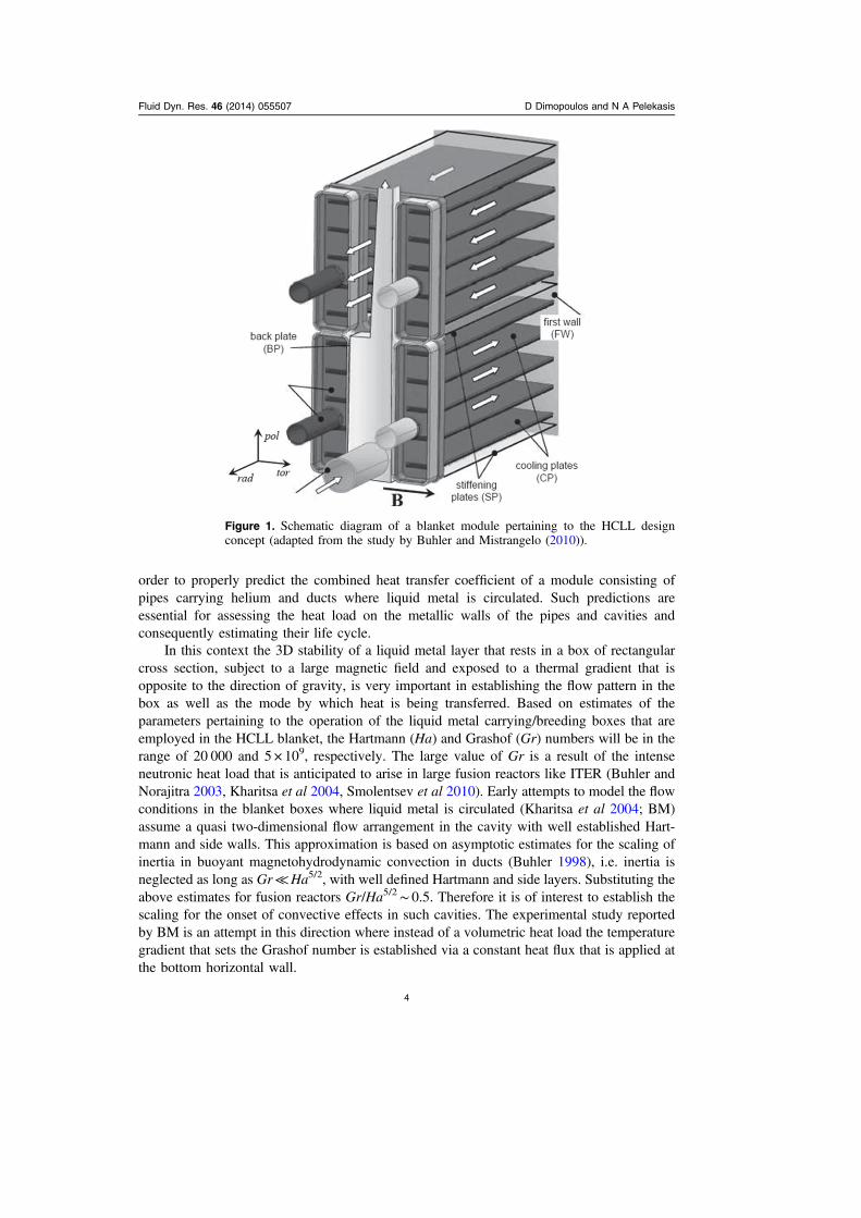
We are interested in studying the three-dimensional stability of a liquid metal layer ofthickness h that rests in a box of rectangular cross section, figure 2. The liquid metal layer isexposed to a strong external magnetic field that is aligned with the long direction of the crosssection. A negative temperature gradient, 2ΔT, is imposed between the bottom and tophorizontal walls that are maintained at different but fixed temperatures, figure 2; ΔT= (Tb−Tt)/2. Stability analysis is expected to provide the waves that will evolve into the standingwave arrangement, see figure 2, discussed by BM.
In this context, quiescent flow conditions prevail in the base flow configuration with alinear temperature profile being established between the two horizontal walls as a result ofheat conduction:
=u a0, (2.1 )0
Fluid Dyn. Res. 46 (2014) 055507 D Dimopoulos and N A Pelekasis
5

Δ= − ′ + = − ′ +( )T T T y h T Ty h T b2 . (2.1 )t b b b0
y′ measures distances from the bottom horizontal wall along the direction perpendicular to itthat is co-linear with gravity, = − g ge
y. Adopting the Boussinesq approximation for density
variations,
ρ ρ β= − − = +⎡⎣ ⎤⎦( ) ( )T T T T T1 , 2, (2.2)b t0 Av Av
which holds whenever temperature variations in the fluid satisfy the condition βΔΤ≪ 1, withβ the thermal expansion coefficient of the operating fluid, the pressure distribution in the staticbase flow arrangement reads as
ρ ρ βΔ= + = − ′ + = ′ − ′′ ′ ′ ′ ′ ⎜ ⎟ ⎜ ⎟⎡⎣⎢
⎛⎝
⎞⎠
⎛⎝
⎞⎠
⎤⎦⎥( )p p gy p p gh T
y
h
y
h, . (2.3)
St0 0 0 0 0 0
2
It is of interest to study the effect of Lorentz forces on the instability pattern of a heatedlayer of liquid metal, i.e. an electrically conducting fluid, in the presence of a magnetic field ofincreasing intensity. To this end, we introduce a uniform horizontal magnetic field of intensity
B that is aligned with the long direction, x, of the layer cross section, = B Be x. The lengthscales of the layer and physical constants of the operating fluid are taken to match thoseemployed in the experimental study by BM, with stainless steel plates forming the Hartmannwalls, electrical conductivity σ≈ 1.37 × 10⁶Ω−1 m−1, copper plates forming the side walls,electrical conductivity σ≈ 5.7 × 10⁷Ω−1 m−1, and a eutectic sodium potassium alloy, Na22K78
with electrical conductivity σ≈ 2.47 × 10⁶Ω−1 m−1, filling the box space between the hor-izontal and vertical walls. Consequently, the magnetic Reynolds number, σμ ν=Rem 0
with
σμ −( )0
1, denoting the magnetic diffusivity of lithium is a very small quantity, the magnetic
induction is negligible and we operate in the low Rem regime. With the onset of free con-vection an electric current density is generated according to Ohm’s law,
σ ϕ ′ = − + ′ × ⎡⎣ ⎤⎦j u B with φ the corresponding electric potential and ′u the emerging
Fluid Dyn. Res. 46 (2014) 055507 D Dimopoulos and N A Pelekasis
6
Figure 2. Schematic diagram of MHD free convection in a rectangular box.
velocity field, and consequently the Lorentz force is exerted per unit volume of the flowing
liquid metal, = ′ × f j B . Finally, in the absence of any electric sources continuity of electriccurrent is satisfied:
ϕ ω ω⋅ ′ = → ′ = ′ ⋅ ′ ≡ × ′
j B u0 , . (2.4)2
Electric current conservation is coupled with continuity and the momentum and heatbalances to provide the description of free convection as a result of the interplay betweenviscous and electromagnetic forces and buoyancy. Introducing characteristic scales for length,time, velocity and pressure based on the layer thickness and buoyant forces,
βΔ ρ βΔ βΔ= ′ ′ ′ = ′ = ′
= ′⎜ ⎟⎛⎝
⎞⎠ ( )
x y zx
h
y
h
z
ht
t
h g Tp
p
g Thu
u
g Tha( , , ) , , , , , , (2.5 )
while scaling temperature and electric potential via the imposed temperature gradient and themagnetic field effects, respectively,
Θ ϕ ϕβΔ
=−−
=T T
T T Bh g Thb, , (2.5 )
b
Av
Av
the three-dimensional problem formulation reads in dimensionless form
⋅ =u 0, (2.6)
∂ ∂
+ ⋅ = − + + − × −( ) ( )u
tu u p Gr u Te
Ha
Grj B , (2.7)y
1 2 22
1 2
∂∂
+ ⋅ =( ) ( )T
tu T
Gr PrT
1, (2.8)
1 22
ϕ ω= ⋅ B . (2.9)2
The no slip and no penetration boundary conditions are imposed on the horizontal andvertical walls of the box, the temperature is fixed at the top and bottom walls while thevertical walls are taken to be thermally insulated:
= = = = = = = = ( ) ( ) ( ) ( )u x u x A u y u y a0 0 1 0, (2.10 )
Θ Θ Θ Θ= = = = − ∂∂
= = ∂∂
= =( ) ( ) ( ) ( )y yx
xx
x A b0 1, 1 1, 0 0. (2.10 )
As regards conduction of electric current in the box walls the thin wall approximation isadopted (Walker 1981),
ϕ ϕ ϕ ϕ− ⋅ = → ∂∂
= = − ∂∂
+ ∂∂
⎛⎝⎜
⎞⎠⎟( )j n c
xx y z c
y za0, , , (2.11 )H s H
22
2
2
2
ϕ ϕ ϕ∂∂
= = ∂∂
+ ∂∂
⎛⎝⎜
⎞⎠⎟( )
xx A y z c
y zb, , (2.11 )H
2
2
2
2
ϕ ϕ ϕ ϕ− ⋅ = → ∂∂
= = − ∂∂
+ ∂∂
⎛⎝⎜
⎞⎠⎟( )j n c
yx y z c
x zc, 0, , (2.11 )S s S
22
2
2
2
Fluid Dyn. Res. 46 (2014) 055507 D Dimopoulos and N A Pelekasis
7
ϕ ϕ ϕ∂∂
= = ∂∂
+ ∂∂
⎛⎝⎜
⎞⎠⎟( )
yx y z c
x zd, 1, (2.11 )S
2
2
2
2
with n signifying the direction normal to the wall pointing outside the box and s2 the 2d
Laplacian operator defined on each one of the walls. Dimensionless parameters cS and cHexpress the intensity of conduction of electric current at the walls in comparison with theliquid metal forming the layer; subscripts s and H denote the side and Hartmann walls andidentify the walls that lie parallel and perpendicular to the magnetic field, respectively. Finallyperiodicity is assumed along the longitudinal direction of the layer:
Θ Θ ϕ ϕ= + ℓ = + ℓ = + ℓ = + ℓ ( ) ( ) ( ) ( )u z u z z z p z p z z z( ) , ( ) , ( ) , ( ) (2.12)
where ℓ denotes the period along the longitudinal direction, z, to be determined via theensuing linear stability analysis. Consequently, the considered geometry does not correspondto a cavity, strictly speaking, nor to a duct. Therefore, in the interest of brevity, we will referto it as a layer, or a box with imposed periodicity in the z direction.
When a solution that is symmetric with respect to the y axis is sought for, the domainalong the x axis ranges from 0 to A/2, in which case symmetry conditions are imposed atx=A/2:
ϕ= ∂∂
= ∂∂
= ∂∂
= ∂∂
= =x Av
x
w
x
T
x xu/2: 0, 0 (2.13)
The following dimensionless quantities govern the dynamics of the flow arrangementunder consideration:
βΔΤν
σρν
να
= = =
= = =
Grg h
Hah B
Pr
AL
hc
c t
chc
c t
ch
, , ,
, , (2.14)HSt St
SCo Co
3
2
202
where α= k/(ρcp) is the thermal diffusivity of the liquid metal, A the aspect ratio of the crosssection and tSt, tCo the thicknesses of the stainless steel and copper walls of the box,respectively. Besides its fundamental importance in studying the role of magnetic fieldintensity and wall electrical conductivity in determining the layer stability, the above setup isintended to simulate as close as possible the flow arrangement studied experimentally by BM.
2.1. Linear stability analysis
We want to examine the stability, of the static flow arrangement characterized by pure heatconduction as described by equations (1.1)–(1.3), which in dimensionless form, read:
Θ ϕ= = − + = − =u y p y y0, 2 1, , 0. (2.15)0 0 0
2
We are looking for a three-dimensional flow pattern that satisfies the formulation outlinedin equations (1.6)–(1.12) and constitutes a small perturbation on the static flow arrangementin equation (1.15). Consequently we assume the standard form:
Fluid Dyn. Res. 46 (2014) 055507 D Dimopoulos and N A Pelekasis
8
Θϕ
Θϕ
Θϕ
= + ≡ω
⎧⎨⎪
⎩⎪
⎫⎬⎪
⎭⎪
⎧⎨⎪⎪
⎩⎪⎪
⎫⎬⎪⎪
⎭⎪⎪
⎧⎨⎪⎪
⎩⎪⎪
⎫⎬⎪⎪
⎭⎪⎪
up
up
u x y
p x y
x y
x y
u u v w
( , )( , )
( , )( , )
e e , ( , , ) (2.16)t ikz
0
0
0
0
1
1
1
1
with Ω=ωr + iωi signifying the complex growth rate while k = 2π/ℓ denotes the wavenumberof the disturbance. Substituting the above anzatz into equations (1.6)–(1.12) we obtain thelinear stability formulation of the problem:
ω = −∂∂
+∂∂
+∂∂
−−⎛⎝⎜
⎞⎠⎟u
P
xGr
u
x
u
yu k (2.17)1
1 1 22
12
21
2 12
ω ϕ= −∂∂
+∂∂
+∂∂
− + − +−⎛⎝⎜
⎞⎠⎟ ( )v
P
yGr
v
x
v
yv k T
Ha
Grv ik (2.18)1
1 1 22
12
212 1
21
2
1 2 1 1
ωϕ
= − +∂∂
+∂∂
− − −∂∂
−⎛⎝⎜
⎞⎠⎟
⎛⎝⎜
⎞⎠⎟w ikP Gr
w
x
w
yw k
Ha
Grw
y(2.19)1 1
1 22
12
21
2 12
2
1 2 11
ωΤ ωΤ+∂∂
= − =∂∂
+∂∂
−− ⎛
⎝⎜⎞⎠⎟v
T
yv
Gr
Pr
T
x
T
yT k2 (2.20)1 1
01 1
1 2 21
2
21
2 12
ϕ ϕϕ
∂∂
+∂∂
− =∂∂
−⎛⎝⎜⎜
⎞⎠⎟⎟x y
kw
yikv (2.21)
21
2
21
2 12 1
1
∂∂
+∂∂
+ =u
x
v
yikw 0 (2.22)1 1
1
The above formulation constitutes an eigenvalue problem in the complex growth rate ωas a function of wavenumber k and the relevant dimensionless parameters identified inequation (1.14), with Θ ϕu p, , , ,1 1 1 1
forming the eigenvector that contains the necessary
information pertaining to the nature of the emerging flow pattern.
3. Numerical methodology
The eigenvalues and eigenvectors of the above linearized problem are calculated by dis-cretizing the perturbation quantities involved in equations (1.17)–(1.22) with the finite ele-ment methodology. The usual biquadratic basis functions, Φi(x,y), are employed for thedescription of all the unknown quantities except for the pressure for which the bilinear basisfunctions, Ψi(x,y), are used (Pelekasis 2006, Dimopoulos and Pelekasis 2012):
∑ ∑
ϕ ϕ
Φ Ψ= == =
⎡
⎣
⎢⎢⎢⎢⎢
⎤
⎦
⎥⎥⎥⎥⎥
⎡
⎣
⎢⎢⎢⎢⎢
⎤
⎦
⎥⎥⎥⎥⎥
uvwT
x y
uvwT
x y P x y p x y( , ) ( , ), ( , ) ( , ); (3.1)i
N
i
i
i
i
i
ii
M
i i
1
1
1
1
1
11
1
Ν, Μ denote the total number of unknowns pertaining to the biquadratic and bilinearbasis functions, respectively, and subscript i denotes the corresponding values at the nodes ofthe two-dimensional mesh spanning the cross section. Subsequently, the standard Galerkin
Fluid Dyn. Res. 46 (2014) 055507 D Dimopoulos and N A Pelekasis
9
finite element methodology provides the weak formulation of the problem. In this fashion theproblem formulation is recast in the form of a matrix eigenvalue problem
ω = ( )B x J x k Gr Ha A c c x; , , , , , (3.2)ij j ij i s H j1 0 1
with B, J signifying the mass and Jacobian matrices, respectively, and x0j, x1j the base solutionand eigenvector, respectively. The eigenvalue ω can be real or complex signifying, when itsreal part becomes positive, the onset of monotonically or periodically growing waves which,upon saturation, will evolve into standing or traveling waves. The eigenvalue problem issolved via the Arnoldi method (Saad 2003) that is employed on a Cayley transform (Cliffeet al 1993) of equation (2.2):
σ ω σ σ
ω σω σ
στ ω σ
− = − → −
= − →−
= −= −
−
( )
( )
J x B x B x B x J B x
B x x
J B B x
( )1
,
1 ( ) (3.3)
ij j ij j ij j ij j ij ij j
ij j i
ij ij ij j
1
Consequently, instead of the original problem described by equation (2.2) the eigenvalueproblem furnishing the largest eigenvalues τ= 1/(ω − σ) is solved via the Arnoldi method,with σ a parameter that affords selection of a specific portion of the spectrum located in thevicinity of value σ. In particular, Hopf bifurcations can be detected, indicating the onset oftraveling waves in the context of the present study, by setting σ to a certain imaginary value.
Inversion of the Jacobian matrix in equation (2.3) constitutes the most time consumingpart of the computation, whereas storing of the Jacobian matrix J determines the dominantstorage requirement of the algorithm. In order to optimize calculations use is made of thebanded nature of the Jacobian and mass matrices J and B in conjunction with the large aspectratio A= L/h of the box cross section. Thus, the Jacobian matrix is stored in a piecemealfashion in a distributed memory environment with each separate memory segment storing asection of the matrix corresponding to a certain segment of the x axis. This entails the entirecolumn of elements along the y direction based on the segment along the x axis. The actualinversion process was performed in the framework provided by the ScaLAPACK softwarelibrary (Blackford et al 1997). In the absence of any strong convective effects we do notemploy any stabilization scheme on the MHD formulation (Planas et al 2011).
3.1. Code validation
In order to ascertain the validity of the above methodology we first investigated the stabilityof a fluid layer resting between two horizontal plates in the absence of a magnetic field, inwhich case we expect to recover the classic Rayleigh–Benárd stability threshold. A neutralstability search was conducted by setting Ha= 0 and calculating the stability threshold, GrCr;the Prandtl number is set to 0.02. In this context, GrCr≈ 42 900, the critical eigenvector wasobtained for kCr= 0 and was characterized by 10 waves along the x direction corresponding toa dimensionless horizontal wavelength of 2D waves on the order of λCr≈Α/10. Since theaspect ratio of the box cross section is set to A = 20 pertaining to the experiments by BM, thedimensional wavelength of the emerging unstable mode is λCr’≈2 h.
Table 1 provides convergence data as well as CPU times upon increasing the number ofprocessors involved in the calculation of GrCr as Ha increases. A mesh of 40 × 20, 60 × 30and 80 × 40 elements was employed whereas the search for GrCr was performed with anincrement ΔGr= 100. It should be stressed that, based on the analytical solution by Reid and
Fluid Dyn. Res. 46 (2014) 055507 D Dimopoulos and N A Pelekasis
10
Harris (1958), the marginal stability of the classic Bénard problem when Ha= 0, is obtained
when ˆ =Ra 1708Cr and corresponds to a wavelength of 2.016 h; = ⋅Ra Gr Pr . In the latter
study ˆ ˆRa Gr, are defined via the temperature difference between the top and bottom hor-izontal plates whereas in the present study ΔΤ is half the temperature difference between the
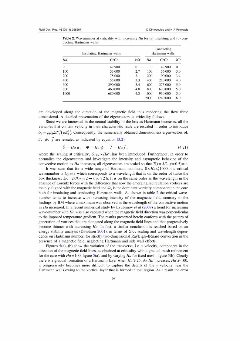
same two plates. Consequently, ˆ =Gr Gr2 and ˆ = = ⋅ ≈Ra Ra Gr Pr2 2 1708Cr CrCr as well.As Ha increases and the Lorentz force effect becomes more pronounced GrCr also increaseswhile the critical wavenumber shifts towards three-dimensional waves with kCr≈ 3 corre-sponding to a dimensionless wavelength λCr≈ 2, i.e. twice the layer thickness.
The geometric and physical constants that are used in the above benchmark tests as wellas in the simulations to be presented in the following with Ha≠ 0, are taken from theexperimental study by BM. Hence, the aspect ratio of the box cross section is taken to beA= 20 with h= 20 mm and the physical properties of the sodium potassium alloy Na22K78 areintroduced in order to determine Gr, Ha and Pr. Pr is a material property, hence it is set to0.02, whereas Gr and Ha also depend on the operating conditions, i.e. the temperaturedifference between the top and bottom walls and the intensity of the applied magnetic field.Following the above experimental study Ha may vary between 100 and 1000 and GrCr ensuesbased on the linear stability analysis results. The latter is a parameter that affords comparisonwith the experimental observations and the available stability analysis results. Finally, in theaforementioned experimental study the conductivity ratios of the Hartmann and side walls,based on the electric conductivities and thicknesses of the containing wall and operatingmedium, are cH= 0.004 15 and cS= 4.5.
Figures 3(a)–(c) portray the temperature eigenvector along with the Ωx and
Ω Ω Ω≡ +y zyz2 2 components of the vorticity eigenvector at criticality; GrCr≈ 53 000,
kCr≈ 3, when Ha= 100. The secondary flow is characterized by a single standing recirculationroll whose vorticity is predominantly aligned with the direction of the magnetic field;
Fluid Dyn. Res. 46 (2014) 055507 D Dimopoulos and N A Pelekasis
11
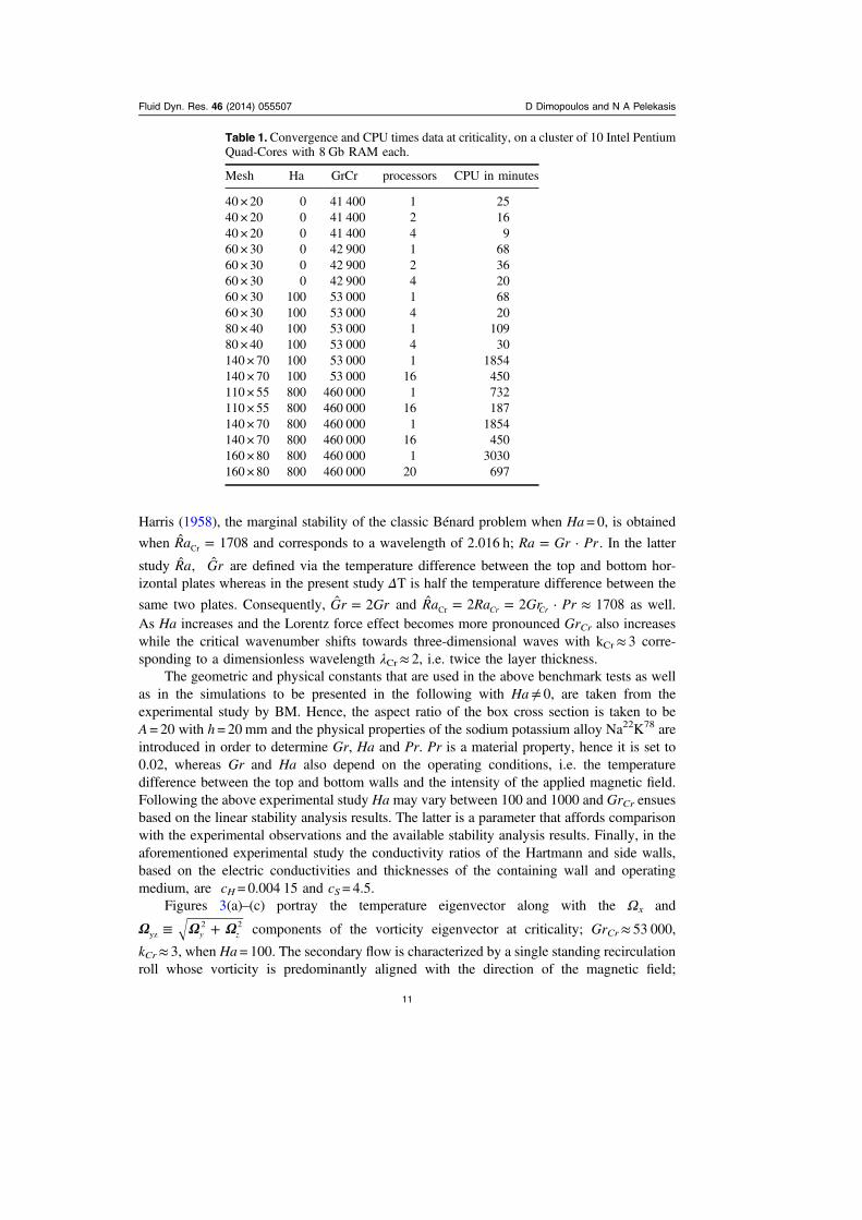
Table 1. Convergence and CPU times data at criticality, on a cluster of 10 Intel PentiumQuad-Cores with 8 Gb RAM each.
Mesh Ha GrCr processors CPU in minutes
40 × 20 0 41 400 1 2540 × 20 0 41 400 2 1640 × 20 0 41 400 4 960 × 30 0 42 900 1 6860 × 30 0 42 900 2 3660 × 30 0 42 900 4 2060 × 30 100 53 000 1 6860 × 30 100 53 000 4 2080 × 40 100 53 000 1 10980 × 40 100 53 000 4 30140 × 70 100 53 000 1 1854140 × 70 100 53 000 16 450110 × 55 800 460 000 1 732110 × 55 800 460 000 16 187140 × 70 800 460 000 1 1854140 × 70 800 460 000 16 450160 × 80 800 460 000 1 3030160 × 80 800 460 000 20 697

figure 3(a) illustrates this behaviour in the temperature eigenvector. Furthermore, x vorticitydominates over the other two vorticity components, as illustrated in figures 3(b), (c), exceptfor the region near the two Hartmann walls where Hartmann layers are formed with sig-nificant variation of the y velocity in the x direction. The above structure persists as the meshis diluted to 60 × 30 or refined to 140 × 70 bi-quadratic elements in the x and y directions,respectively. It should also be stressed that, as Ha increases, simulations are performedincorporating symmetry conditions with respect to the x=A/2 plane, in order to increase theaccuracy of the calculations. Figures 3(d), (e) illustrate the x and yz components of thevorticity vector calculated in this fashion. The results accurately reproduce those obtainedwhen the full cross-section of the box is discretized, shown in figures 3(b), (c). Formation ofHartmann layers is manifested in the abrupt change of x vorticity as the Hartmann walls areapproached, figures 3(b), (d) but also in the narrow strip of large yz vorticity that is clearlycaptured by zooming in that same region of the yz vorticity contours, figures 3(e), (f). Thebulk of the results presented in the next section are obtained using the symmetry condition
Fluid Dyn. Res. 46 (2014) 055507 D Dimopoulos and N A Pelekasis
12
Figure 3. (a) Temperature, (b) x vorticity and (c) yz vorticity contours when Ha = 100with a mesh of 110 × 55 elements. (d), (e) reproduce the results in (b), (c) by using thesymmetry condition and (f), (g) provide a focus of the yz vorticity shown in (c), (e),respectively, in the vicinity of the left Hartmann wall.
provided in equation (1.15). This is a well justified approach since in all cases considered thedominant eigenmode at criticality is symmetric with respect to the x =A/2 plane.
4. Results and discussion
In this section an extensive parametric study is performed in order to examine the neutralstability characteristics of the Rayleigh–Bénard instability as Ha increases. The structure ofthe emerging eigenvector is of interest. In particular, the scaling of GrCr with Ha is sought inconjunction with the associated dominant force balance that produces it, and the possibilityfor Hartmann and side layers to develop in this limit is investigated. The effect of wallconductivity in determining the stability is examined by parametrically varying the electricalconductivity of Hartmann and side walls.
The neutral stability data provided in the following were mostly obtained with a mesh of110 × 55 biquadratic elements along the x and y directions. Numerical convergence wasascertained with a mesh of 140 × 70 biquadratic elements in our local cluster of 16 processors.The eigenvectors presented in the following subsections were obtained at criticality, i.e. whenGr=GrCr. Throughout the parametric study that was conducted no complex eigenvalues weredetected and the symmetric eigenmode dominated the stability of the box, signifying the onsetof a standing wave type flow arrangement upon saturation.
4.1. Asymptotic behavior as Ha increases
Before we proceed with the presentation of the results of the numerical stability analysis, itwill be useful to obtain an order of magnitude estimate of the emerging flow arrangement atcriticality in the limit Ha≫ 1. Anticipating standing waves to dominate the neutral stabilityregime, based on the available measurements by BM, the growth rate ω is set to zero and thevelocity is rescaled to reflect the balance between the Lorentz force and buoyancy
Δρβ σ= ′ → =
( )
Uu
g T BU u
Ha
Gr. (4.1)
02
2
1 2
The rest of the problem variables whose scaling involves the characteristic velocity arerescaled accordingly:
Φ ϕ= = Ha
GrJ j
Ha
Gr, (4.2)
2
1 2
2
1 2
with capital letters denoting rescaled variables. Temperature and pressure are not rescaledsince they are determined by the temperature difference between the two horizontal walls.Upon substitution in equations (1.17)–(1.22) the stability formulation reads at criticality:
= −∂∂
+∂∂
+∂∂
−⎛⎝⎜
⎞⎠⎟
P
x Ha
U
x
U
yU k0
1(4.3)1
2
21
2
21
2 12
Φ= −∂∂
+∂∂
+∂∂
− + − +⎛⎝⎜
⎞⎠⎟ ( )
P
y Ha
V
x
V
yV k T V ik0
1(4.4)1
2
21
2
21
2 12
1 1 1
Φ= − +
∂∂
+∂∂
− − −∂∂
⎛⎝⎜
⎞⎠⎟
⎛⎝⎜
⎞⎠⎟ikP
Ha
W
x
W
yW k W
y0
1(4.5)1 2
21
2
21
2 12
11
Fluid Dyn. Res. 46 (2014) 055507 D Dimopoulos and N A Pelekasis
13
∂∂
=∂∂
+∂∂
−− ⎛
⎝⎜⎞⎠⎟V
T
y
Ha Gr
Pr
T
x
T
yT k (4.6)1
02 1 2
12
21
2 12
Φ Φ
Φ Ω⋅ = →∂∂
+∂∂
− =∂∂
− =⎛⎝⎜
⎞⎠⎟J
x yk
W
yikV a0 , (4.7 )x1
21
2
21
2 12 1
1 1
Ω = × U b(4.7 )
∂∂
+∂∂
+ =U
x
V
ykWi 0; (4.8)1 1
1
the boundary conditions are not affected by the rescaling and they retain the form prescribedby equations (1.10)–(1.13). In the following, subscript 1 identifies the linearized part of thevariables and is dropped for convenience. Convective effects survive in the energy balance inthis limit and will be seen in the following that, for perfectly conducting walls, play animportant role in setting up the vorticity distribution in the bulk of the box. Inertia effects areO(1/Ha2) in this limit but drop out of the momentum balance of linear stability, in the absenceof any base flow. With the above rescaling Lorentz and buoyancy forces balance each other iny momentum. Furthermore, since it is a thermal instability that produces the convectivemotion, in order for any appreciable temperature difference to appear in the box heat diffusionshould balance convection in the energy conservation equation (3.6). Consequently, weanticipate that GrCrPr =RaCr∼Ha2 at criticality, which provides the relevant scaling for theconvective instability to arise in the flow arrangement under consideration. It is in this limit
that the characteristic velocity Δρβ σ ν≡ =( ) ( ) ( )U g T B Gr Ha h0 02 2 remains on the same
order of magnitude for fixed operating liquid metal and fixed layer thickness. Τhe abovescaling of RaCr∼Ha2 was also identified as the dominant balance for the onset of buoyancydriven convection in a cylindrical shell with electrically insulating walls in the presence of amagnetic field by Davoust et al (1999).
In this context as Ha increases a core region develops where buoyancy balances Lorentzforces and viscous effects can be neglected. It is however important to ascertain under whatconditions the flow will assume a quasi two-dimensional structure in the core region wherethe vorticity vector is more or less aligned with the magnetic field, i.e. along x direction, andexhibits negligible variationalong magnetic field lines, while the y and z vorticity componentsremain subdominant. To this end, and adopting a similar approach as the one presented by
Buhler (1998), we introduce the vorticity vector Ω
by taking the cross product ofequations (3.3)–(3.5):
Ω× = + + × → + ∂∂
− + ∂∂
=⎜ ⎟⎛⎝
⎞⎠
P
HaU Te J e
Ha xJ kTe
T
xe
1 1i 0; (4.9)y x x z2
22
2
≡ + + ∂∂
∂∂
f e e kfeix
f
x yf
y zin the context of the linearized problem statement. Taking the limit
as Ha→∞ and invoking Ohm’s law we obtain the variation of the electric potential alongmagnetic field lines:
Fluid Dyn. Res. 46 (2014) 055507 D Dimopoulos and N A Pelekasis
14
∫∫
∫∫ ∫
Φ Φ
Φ
Φ Φ
∂∂
= − → ∂∂
= ⟹ ∂∂
= →
= +
=
xkT
rdr
k T rx
k Tdr
k p Tdr
i
i d
i
i d
. (4.10)
A
x
x
A
at x A
symmetry
x
x
A
x
x
p
A
2
22
2
2
2
2
2
00
2
Substituting equation (3.10) in the charge conservation equation (3.7) we obtain thevorticity component in the direction of the magnetic field, Ωx:
∫ ∫
∫ ∫
Ω Φ
Φ
= +
= + −
≡ ∂∂
+
⊥
⊥
⊥
( )
k p T r
k p V r
f ef
ye ikf
i d d
i d 2 d ,
, (4.11)
x
x
p
A
x
p
A
y z
2
0
22
2
0
2
with Φ denoting the value of the electric potential at the Hartmann walls.Therefore, generation of x vorticity in the core is governed by the upward fluid motion
due to buoyancy and is modulated by the electric current motion in the Hartmann layersdepending on their electrical conductivity. Based on x momentum there is no pressure drop inthe core as Ha→∞ and the x component of velocity will be very small to leading order.Based on continuity and the y and z momentum equations, V and W dominate in the corecorresponding to a recirculation pattern that is aligned with the magnetic field, while the othertwo components of vorticity remain subdominant. The relative importance of the two termson the right hand side of equation (3.11) will determine the degree of two dimensionality ofthe x-vorticity of the flow.
The flow arrangement in the Hartmann layer is determined by the balance betweenmagnetic and viscous forces in y momentum, thus generating a layer of thickness on the orderof Ha−1. Consequently, continuity is accommodated with V, W remaining O(Ha) or O(1)whereas U is O(1) or O(Ha−1), depending on the electrical conductivity of the Hartmannwalls, for mass balance to be satisfied in the Hartmann layer. Furthermore, the charge con-servation equation (3.7a) provides the scaling for the x component of the electric current in theHartmann layer, JHx =O(1) or O(Ha−1) for electrically insulating and conducting walls,respectively. This is necessary in order to balance the y component, JHy, that remains O(Ha)or O(1) inside the Hartmann layer in the same context. In particular, when the Hartmann wallsare poor conductors only a small portion of the electric current can pass through them, seealso boundary condition (1.11a), (1.11b). Rather, it turns inside the Hartmann layer to reachthe side walls. On the contrary, when the Hartmann walls are good conductors the currentloops close within the core region while the induced currents in the Hartmann layer remainweak. The above arguments are corroborated upon introducing corrections for variableswithin the Hartmann layer and rescaling charge conservation equation in the Hartmann layerin order to obtain the dominant balance for the total x vorticity:
Fluid Dyn. Res. 46 (2014) 055507 D Dimopoulos and N A Pelekasis
15
Φ Φ Ω Ω
Φ
Ω
Φ
Φ
Φ
Ω
∂∂
∂∂
∂∂
∂∂
∂∂
∂∂
∂∂
+ = + →
=
≡ →
= −
= −
=
= −
= −
− −
−
Ha X Ha X
Xx
HaJ
x
HaX
J
x
HaJ
X
HaX
1 1
,
and
. (4.12)
Hx xH
Hx
Hx
H
H Hx
Hx
H
Hx
2
2
22
2
2
2
1
22
2
In the above ΩΗx and JHx denote the viscous corrections of x vorticity and the x com-ponent of electric current, X is the stretched wall normal coordinate inside the Hartmann layer,whose order of magnitude varies depending on the conductivity of the Hartmann walls. Thus,substituting in the vorticity equation (3.9) we obtain
Ω Ω ΩΩ
∂∂
+∂∂
+∂∂
− = →∂∂
+∂∂
=∂∂
− =X
J
x
J
xikT
X
J
x X0 0. (4.13)Hx Hx x Hx Hx Hx
Hx
2
2
2
2
2
2
Requiring that the x-vorticity, Ωx+ΩHx, vanishes at the Hartmann wall, i.e. at X = 0, andthat ΩΗx vanishes as X→∞ the viscous correction of the x component of vorticity andelectric current are recovered as
Ω Ω
Ω
Ω
Ω
Ω
= − =∂∂
= − →
= −∂∂
→
= −∂∂
= −
−
=
==
=−
=
( )x e
HaJ
XHa J
XJ
x
Ha
0
. (4.14)
Hx xX
HxHx Hx X
Hx
X
Hx X
H
x
x x
0
00
0
1
0
Finally the electric potential at the Hartmann walls can be calculated by invoking the thinwall boundary condition equations (1.11a), (1.11b)
Φ Φ Φ Φ
Φ Ω Φ
Φ
− = ∂∂
+∂∂
→ ∂∂
= − − → − ∂∂
= +
⊥= = =
⊥−
==
−⊥( )
cx x x
c Hax
c Ha . (4.15)
Hx
H
x x
H x xx
H
2
0 0 0
2 1
00
1 2
Upon substitution in (3.10) the value of the electric potential at the wall can be calculatedand through it the x-vorticity component distribution in the bulk of the liquid metal layer:
Fluid Dyn. Res. 46 (2014) 055507 D Dimopoulos and N A Pelekasis
16
∫ ∫Φ Φ− = + ∇ → = −+
−⊥ ⊥ −( )k T r c Ha
c Hak T ri d
1i d (4.16)
A
HH
A
0
21 2 2
10
2
∫ ∫ ∫Ω = −+
+ −− ( )c Ha
k T r k p V r1
i d i d 2 d . (4.17)xH
A x
p
A
10
2
0
2
Coupling of equation (3.16) with (3.10) provides the electric potential in the box with amaximum in the Hartmann layer region for insulating walls, Φ∼Ηα, or in the core regionwhen they are highly conducting, Φ∼Ο(1). Furthermore, coupling with the solution in theside layer provides the electric potential at the Hartmann wall in the form of a quadraticprofile that vanishes at the side walls. Equation (3.17) clearly illustrates the importance ofwall conductivity in determining the Hartmann braking effect and its role in establishing theflow arrangement inside the box. To this end it will be useful to note that the vertical andtransverse velocity components in the core read:
Φ= − + − ∂∂
V k TP
yai , (4.18 )
Φ= ∂∂
−Wy
kP bi . (4.18 )
Next, upon taking the divergence of y and z momentum, equations (3.4) and (3.5),pressure variations in the vertical plane are associated with temperature gradients in the box:
= ∂∂⊥ PT
y; (4.19)2
in deriving the last equation continuity was employed, combined with the fact that as Haincreases pressure variations in the longitudinal direction vanish, see also equation (3.3), andconsequently the longitudinal velocity component U tends to vanish as well inside the core.Thus, pressure variations in the core remain O(1) as Ha increases whereas V, W scale like
+ −( )c Ha1 H1 . In fact, matching with the flow inside the Hartmann layer recovers this
scaling. Clearly then, the vorticity variation inside the Hartmann layer will be much moredifficult to capture numerically when the Hartmann walls are insulating, in which case V hasto vary from O(Ha) to zero at the wall within a layer whose thickness shrinks like Ha−1. Onthe other hand when the Hartmann walls are highly conducting the transverse velocity V is onthe order of 1/ cH, a Hartmann layer of very weak vorticity is formed in their vicinity andcalculations can proceed to quite large Ha values without loss of accuracy. Similar argumentshold for the velocity component parallel to the side walls when they are highly conducting.The above aspects of the flow are corroborated by numerical findings in the present study.
Variation of x vorticity along the magnetic field lines, in the fashion prescribed byequation (3.17), bears significance on the validity of the assumption of quasi 2D flowarrangement inside the box. When the Hartmann walls are highly conducting both terms onthe right-hand side of equation (3.17) are O(1) as Hartmann increases. Consequently, thevolume integral of thermally induced vertical motion in the box is equally important with thesurface gradient of the electric potential and x vorticity varies significantly along the magneticfield lines. In the vicinity of Hartmann walls their conductivity cH determines the local electriccurrents leading to a transverse velocity that is much smaller than its value in the bulk, inwhich case the volume integral dominates. When poor conducting Hartmann walls areconsidered, cH≈ 0, strong electric potential gradients form within the Hartmann layers withthe combined conductivity determined by Ha−1. Consequently, x-vorticity is O(Ha) in thevicinity of the Hartmann walls but transverse velocity V is also O(Ha) in this case throughout
Fluid Dyn. Res. 46 (2014) 055507 D Dimopoulos and N A Pelekasis
17
the liquid metal layer. As a result the volume integral in equation (3.17) is equally importantas the Hartmann braking effect within the Hartmann layers and x-vorticity exhibits significantvariation along the magnetic field lines. Heat being transferred by convection in the coredetermines the vorticity component in the x direction and the flow in the box is essentiallythree dimensional. Consequently, the quasi 2D assumption is not applicable at the onset ofthermal convection in the presence of a strong magnetic field, in which case Ra∼Ha2.Simulations presented in subsequent sections confirm this behavior but also illustrate thecentral role played by discrepancies in the electrical conductivities of the Hartmann and sidewalls, οn the structure of the emerging flow pattern as well as the onset of high velocity jets inthe box side layers.
It should also be stressed that in the case of insulating walls more intense electriccurrents, Jx, JHx∼O(1), develop within the bulk of the flow (equation (3.15)) and the Hart-mann layers (equation (3.14)) as the intensity of the magnetic field is raised. In the samecontext of poor Hartmann wall conductivity electric currents along the y and z directionsremain O(Ha) in order to satisfy continuity of electric current in the Hartmann layers. Thesecurrents are associated with large electric potential gradients leading to O(Ha) transverse andspanwise velocities. As will be seen in the results and discussion section, this motion iscomplemented by strong side wall velocities at the box corners in order to satisfy masscontinuity. The above described pattern constitutes the magneto-hydrodynamic pumpingeffect. Finally, the electric currents along the x, y and z directions in the Hartmann layers areof the same order of magnitute in Ha as in the bulk of the flow hence electric currents need togo into the Hartmann layers before they turn to reach the side walls. On the contrary, whenconducting Hartmann walls are considered, cH≫Ha−1, the y and z components of the electriccurrent are O(1) in the bulk of the box except in the vicinity of the Hartmann layers wherethey are very small O(1/ cH). The x component of the electric current is O(1) in the core,equation (3.10), and remains very small, O(Ha−1), within the Hartmann layers in order tobalance electric currents in the transverse and spanwise directions. Consequently the electriccurrent loops remain O(1) and close within the core region in this case, considering that sidewalls are taken to be highly conductive at all cases in the present study.
The flow arrangement is completed by the analysis of the region located near the sidewalls of the box. In this case, coupling of the linearized x vorticity equation (3.9) with thecharge conservation equation (3.7b) in the limit as Ha→∞, provides the following dominantbalance in the vicinity of the two side walls:
Φ Φδ δ
∂∂
+∂∂
= ≡Ha Y x
Yy1
0 (4.20)S S2 4
4
4
2
2
along with the scaling, Δ=Ηa−1/2, of the rapidly varying part of the electric potential, ΦS,inside the bottom side layer. Consequently, U =O(Ha) so that continuity is satisfied near thecorner region as fluid rises up from the Hartmann layers. Thus, the x velocity acquires largevalues in this region where pressure driven flow exists such as ∂ ∂ =P x O (1) from x-momentum (equation (3.3)), while the box acts as a magnetohydrodynamic pump generatingan O(Ha1/2) flow rate, UΔ, within the side layers in the direction of the magnetic field. Thisflow pattern develops in parallel to the circulatory motion in the core and has the potential tointeract with it, in which case it constitutes an active side layer. The analysis by Buhler (1998)of free convection MHD flow in cavities anticipated formation of high speed jets even whenboth Hartmann and side walls are perfectly conducting. However, as will also be seen in thenext sections, in the present study we only obtain side layer formation accompanied bysignificant side wall motion when the Hartmann walls are poorly conducting, in agreementwith older studies of pressure driven flow in ducts (Walker 1981).
Fluid Dyn. Res. 46 (2014) 055507 D Dimopoulos and N A Pelekasis
18

4.2. Numerical investigation of neutral stability as Ha increases
An extensive numerical investigation was carried out in order to obtain the neutral stability ofthe box. As illustrated in figures 6(a), (b) showing the neutral stability curve for insulating,cH= 0.004 15, and conducting, cH= 4.5, Hartmann walls, respectively, the critical value of Grscales like Ha2 with increasing Hartmann number, signifying the balance between buoyancyand Lorentz forces. No complex eigenvalues were detected at or beyond criticality. Conse-quently all the unstable eigenmodes correspond to the onset of standing periodic waves. Ascan be gleaned from figure 4(a) the experimental results pertaining to criticality also obey thisscaling. In fact, this pattern, i.e. GrCr∼Ha2, persists even when the Hartmann walls areequally conducting as the side walls, cH= cS= 4.5, as illustrated by figure 4(b). However,discrepancies in the electrical conductivities of the Hartmann and side walls bears significancein the nature of the dominant eigenvector at criticality. As was pointed out by the asymptoticanalysis and will be verified by numerical calculations of the dominant eigenvectors thecombined conductivity of the Hartmann walls and Hartmann layers, cH+Ha
−1, controls thestrength of the vortical motion within the Hartmann layers. Furthermore, owing to theintensity of the buoyant motion in the core at criticality, appreciable variations of x-vorticity
Fluid Dyn. Res. 46 (2014) 055507 D Dimopoulos and N A Pelekasis
19
Figure 4. Neutral stability diagrams: (a) insulating Hartmann walls and (b) conductingHartmann walls.
are developed along the direction of the magnetic field thus rendering the flow threedimensional. A detailed presentation of the eigenvectors at criticality follows.
Since we are interested in the neutral stability of the box as Hartmann increases, all thevariables that contain velocity in their characteristic scale are rescaled in order to introduce
Δρβ σ= ( )U g T B0 02 . Consequently, the numerically obtained dimensionless eigenvectors of,
ϕ u j, , are rescaled as indicated by equation (3.2),
Φ ϕ = = = U Ha u Ha J Ha j, , , (4.21)
where the scaling at criticality, GrCr∼Ha2, has been introduced. Furthermore, in order tonormalize the eigenvectors and investigate the intensity and asymptotic behavior of theconvective motion as Ha increases, all eigenvectors are scaled so that T(x =A/2, y= 0.5) = 1.
It was seen that for a wide range of Hartmann numbers, 0 <Ha⩽ 1000, the criticalwavenumber is kCr≈ 3 which corresponds to a wavelength that is on the order of twice thebox thickness, λCr= 2π/kCr≈ 2→ λ′Cr≈ 2 h. It is on the same order as the wavelength in theabsence of Lorentz forces with the difference that now the emerging recirculation vortices aremainly aligned with the magnetic field and Ωx is the dominant vorticity component in the coreboth for insulating and conducting Hartmann walls. As shown in table 2 the critical wave-number tends to increase with increasing intensity of the magnetic field, contrary to thefindings by BM where a maximum was observed in the wavelength of the convective motionas Ha increased. In a recent numerical study by Lyubimov et al (2009) a trend for increasingwave-number with Ha was also captured when the magnetic field direction was perpendicularto the imposed temperature gradient. The results presented herein conform with the pattern ofgeneration of vortices that are elongated along the magnetic field lines and that progressivelybecome thinner with increasing Ha. In fact, a similar conclusion is reached based on anenergy stability analysis (Davidson 2001), in terms of GrCr scaling and wavelength depen-dence on Hartmann number, for strictly two-dimensional Rayleigh–Bénard convection in thepresence of a magnetic field, neglecting Hartmann and side wall effects.
Figures 5(a), (b) show the variation of the transverse, i.e. y velocity, component in thedirection of the magnetic field lines, as obtained at criticality with a gradual mesh refinementfor the case with Ha = 100, figure 5(a), and by varying Ha for fixed mesh, figure 5(b). Clearlythere is a gradual formation of a Hartmann layer when Ha⩾ 25. As Ha increases, Ha≫ 100,it progressively becomes more difficult to capture the details of the y velocity near theHartmann walls owing to the vortical layer that is formed in that region. As a result the error
Fluid Dyn. Res. 46 (2014) 055507 D Dimopoulos and N A Pelekasis
20
Table 2. Wavenumber at criticality with increasing Ha for (a) insulating and (b) con-ducting Hartmann walls.
Insulating Hartmann wallsConducting
Hartmann walls
Ha GrCr kCr Ha GrCr kCr
0 42 900 0 0 42 900 0100 53 000 2.7 100 56 000 3.0200 75 000 3.1 200 90 000 3.4400 155 000 3.3 400 210 000 4.0600 290 000 3.4 600 375 000 5.0800 460 000 4.0 800 620 000 5.01000 680 000 4.3 1000 930 000 5.0
2000 3240 000 6.0
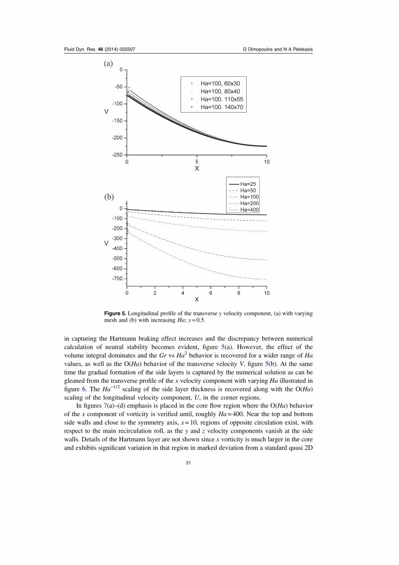
in capturing the Hartmann braking effect increases and the discrepancy between numericalcalculation of neutral stability becomes evident, figure 5(a). However, the effect of thevolume integral dominates and the Gr vs Ha2 behavior is recovered for a wider range of Havalues, as well as the O(Ha) behavior of the transverse velocity V, figure 5(b). At the sametime the gradual formation of the side layers is captured by the numerical solution as can begleaned from the transverse profile of the x velocity component with varying Ha illustrated infigure 6. The Ha−1/2 scaling of the side layer thickness is recovered along with the O(Ha)scaling of the longitudinal velocity component, U, in the corner regions.
In figures 7(a)–(d) emphasis is placed in the core flow region where the O(Ha) behaviorof the x component of vorticity is verified until, roughly Ha = 400. Near the top and bottomside walls and close to the symmetry axis, x= 10, regions of opposite circulation exist, withrespect to the main recirculation roll, as the y and z velocity components vanish at the sidewalls. Details of the Hartmann layer are not shown since x vorticity is much larger in the coreand exhibits significant variation in that region in marked deviation from a standard quasi 2D
Fluid Dyn. Res. 46 (2014) 055507 D Dimopoulos and N A Pelekasis
21
Figure 5. Longitudinal profile of the transverse y velocity component, (a) with varyingmesh and (b) with increasing Ha; y= 0.5.
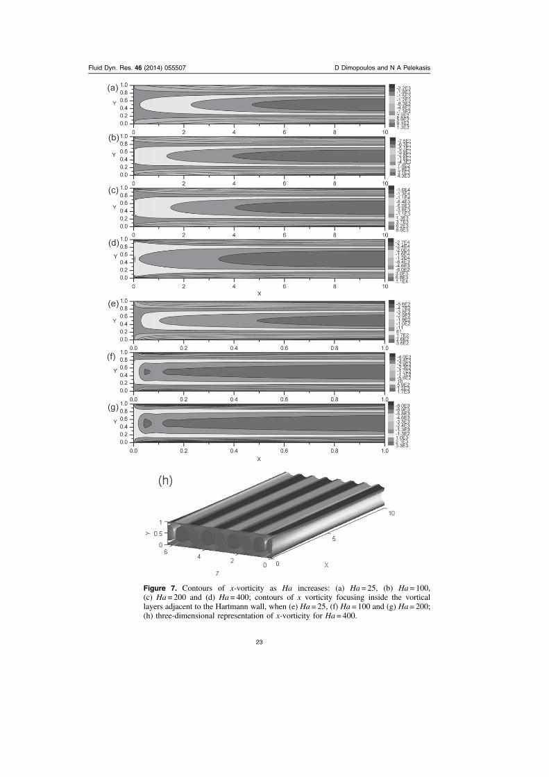
arrangement. Formation of a Hartmann layer is illustrated in figures 7(e), (f), (g), that zoom innear the left side of the box, where vorticity has to drop down to zero at the Hartmann walls.Figure 7(h) provides a three-dimensional representation of x vorticity at criticality whenHa= 400, illustrating an array of four pairs of counter rotating vortices that emerge when alarge enough temperature gradient is achieved for fixed magnetic field and operating liquid.Within one period of the standing wave it assumes the form of two counter-rotating vorticesthat are aligned with the magnetic field. Warm and cold patches of fluid are situated onopposite ends of each vortex causing ascending and descending fluid motion respectively.
The above flow arrangement is also reflected in the evolution of the electric potentialwith Ha, figures 8(a)–(d), which exhibits negligible variation near the two side walls, asexpected owing to their large conductivity ratio, while varying in the region occupied by theHartmann layers indicating the tendency of electric currents to enter that region. The latter is amanifestation of the poor conductivity ratio of the Hartmann walls, where a quadratic var-iation is established as Ha increases, in agreement with equation (3.16). The O(Ha) growth ofthe electric potential in the Hartmann layers is also captured in the panel sequence shown infigure 8. The activity in the Hartmann layer generates significant Lorentz forces,
× = × J B J e ez z y, and is responsible for maintaining a large transverse velocity, V, in the
region near the Hartmann walls in a manner that can be identified as electromagnetic pumping(Davidson 2001). Figure 9(a) shows the uniformity of electric current in the core region aswell as charge motion along and perpendicular to the Hartmann layers near the two cornerregions when Ha = 25, in which case the Hartmann layer is first observed; see also figure 5(b).The electric current loops have to go through the Hartmann layers before they close, asillustrated in figure 9(a), and the details of the flow in these regions are essential for por-traying the electric current motion in the xy plane. Figure 9(b) provides a snapshot of theelectric current loop on a Hartmann wall indicating closure of the current paths away from thehighly conducting side walls at Y= 0, 1, in the core region and at the center of the recircu-lation vortices.
Fluid Dyn. Res. 46 (2014) 055507 D Dimopoulos and N A Pelekasis
22
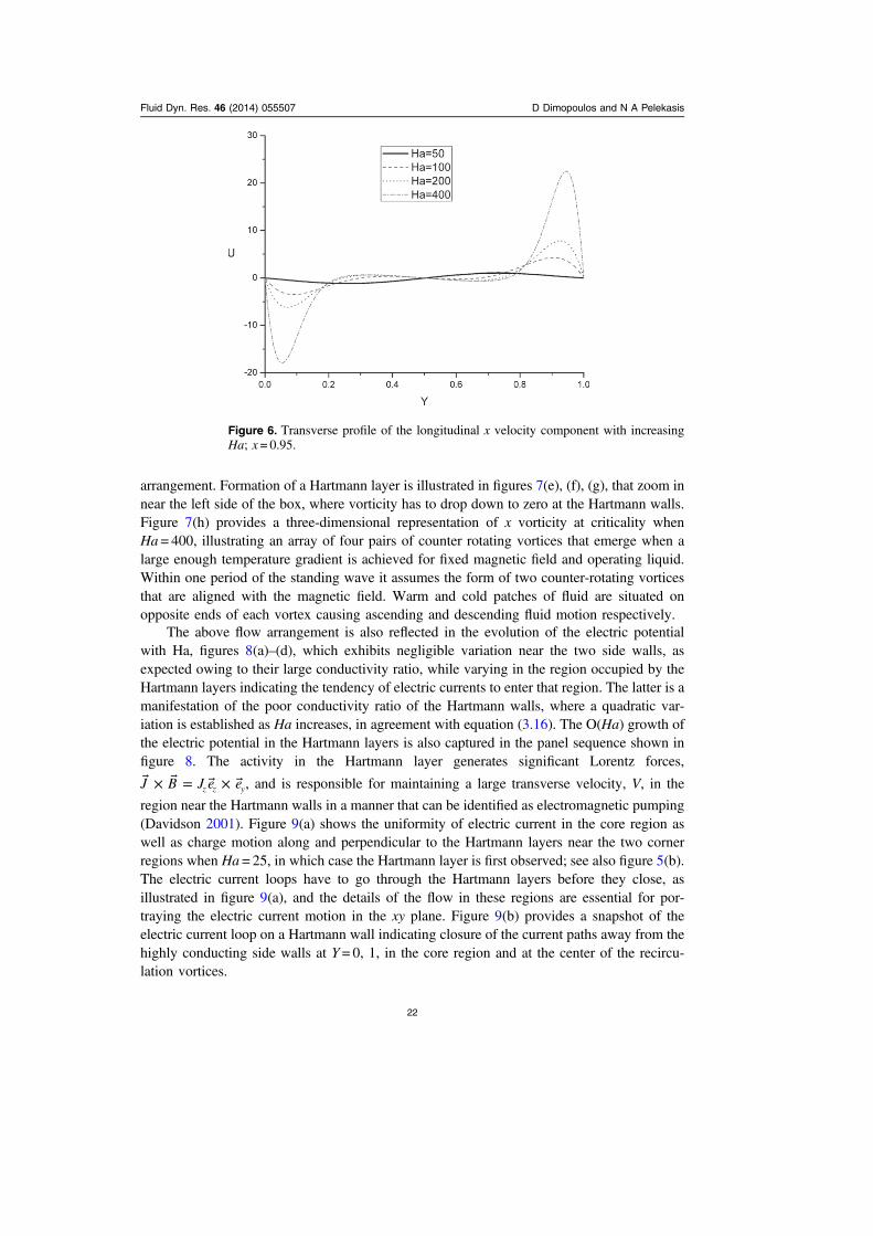
Figure 6. Transverse profile of the longitudinal x velocity component with increasingHa; x= 0.95.
Fluid Dyn. Res. 46 (2014) 055507 D Dimopoulos and N A Pelekasis
23
Figure 7. Contours of x-vorticity as Ha increases: (a) Ha= 25, (b) Ha= 100,(c) Ha= 200 and (d) Ha= 400; contours of x vorticity focusing inside the vorticallayers adjacent to the Hartmann wall, when (e) Ha = 25, (f) Ha = 100 and (g) Ha= 200;(h) three-dimensional representation of x-vorticity for Ha= 400.
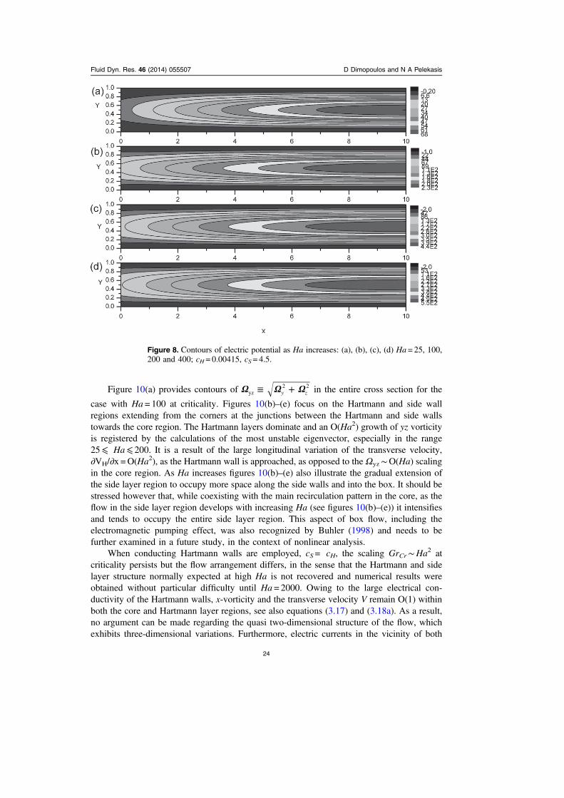
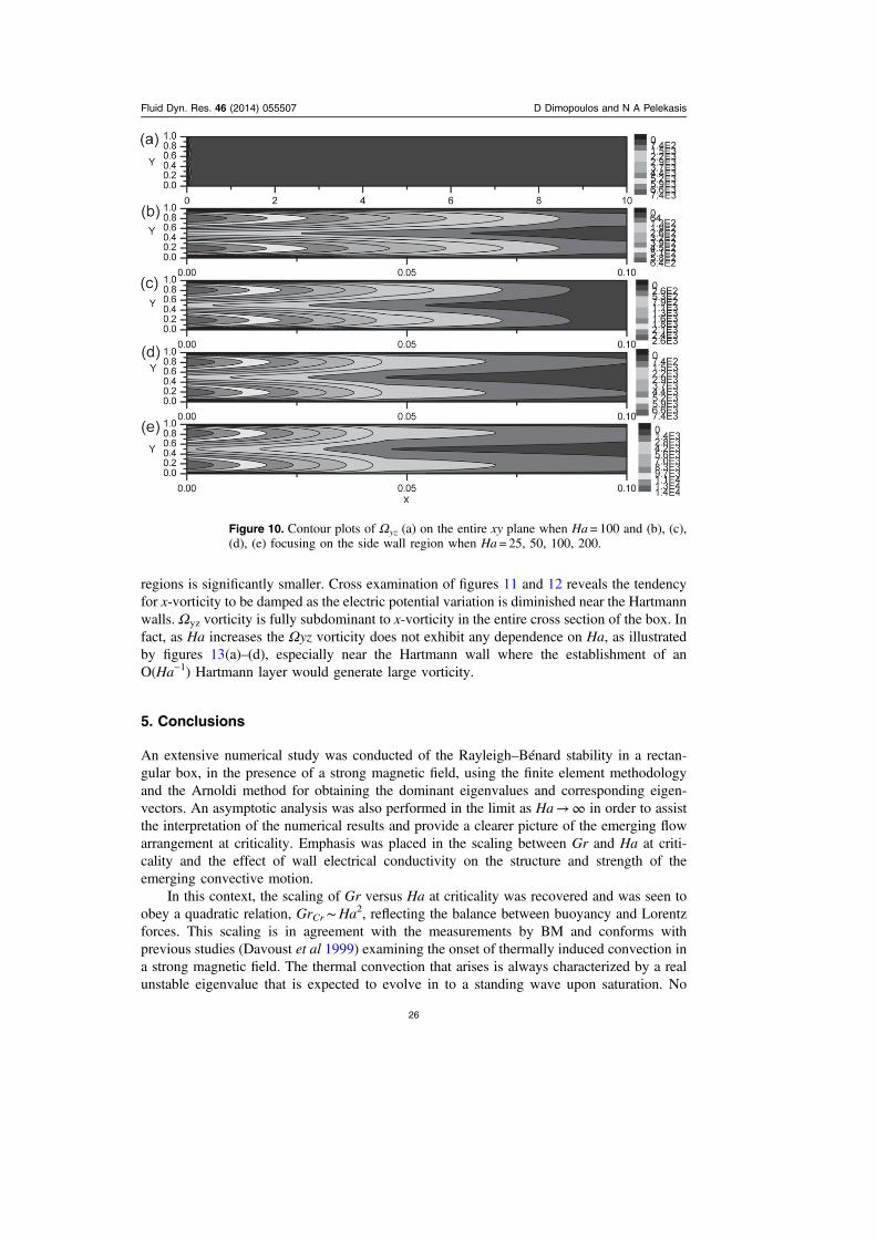
Figure 10(a) provides contours of Ω Ω Ω≡ +y zyz2 2 in the entire cross section for the
case with Ha = 100 at criticality. Figures 10(b)–(e) focus on the Hartmann and side wallregions extending from the corners at the junctions between the Hartmann and side wallstowards the core region. The Hartmann layers dominate and an O(Ha2) growth of yz vorticityis registered by the calculations of the most unstable eigenvector, especially in the range25⩽ Ha⩽ 200. It is a result of the large longitudinal variation of the transverse velocity,∂VH/∂x =O(Ha2), as the Hartmann wall is approached, as opposed to the Ωyz∼O(Ha) scalingin the core region. As Ha increases figures 10(b)–(e) also illustrate the gradual extension ofthe side layer region to occupy more space along the side walls and into the box. It should bestressed however that, while coexisting with the main recirculation pattern in the core, as theflow in the side layer region develops with increasing Ha (see figures 10(b)–(e)) it intensifiesand tends to occupy the entire side layer region. This aspect of box flow, including theelectromagnetic pumping effect, was also recognized by Buhler (1998) and needs to befurther examined in a future study, in the context of nonlinear analysis.
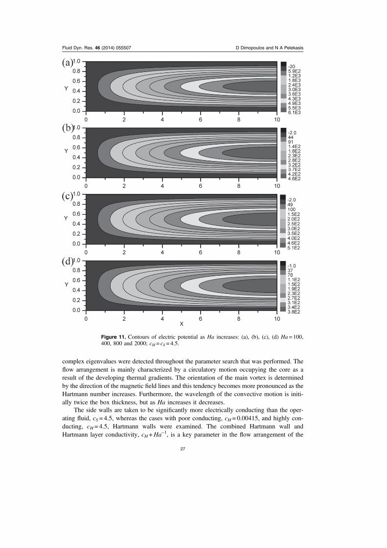
When conducting Hartmann walls are employed, cS= cH, the scaling GrCr∼Ha2 atcriticality persists but the flow arrangement differs, in the sense that the Hartmann and sidelayer structure normally expected at high Ha is not recovered and numerical results wereobtained without particular difficulty until Ha = 2000. Owing to the large electrical con-ductivity of the Hartmann walls, x-vorticity and the transverse velocity V remain O(1) withinboth the core and Hartmann layer regions, see also equations (3.17) and (3.18a). As a result,no argument can be made regarding the quasi two-dimensional structure of the flow, whichexhibits three-dimensional variations. Furthermore, electric currents in the vicinity of both
Fluid Dyn. Res. 46 (2014) 055507 D Dimopoulos and N A Pelekasis
24
Figure 8. Contours of electric potential as Ha increases: (a), (b), (c), (d) Ha= 25, 100,200 and 400; cH = 0.00415, cS= 4.5.

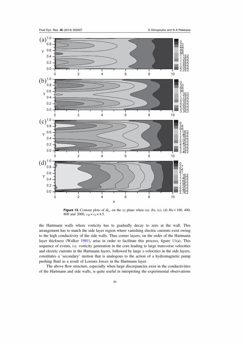
Hartmann and side walls are negligible and the electric current loops close within the coreregion. This is in accordance with the analysis presented in subsection 4.1 indicating thesignificant reduction in y velocity in the vicinity of highly conducting Hartmann walls. Thistype of flow arrangement is distinctly different from the one outlined for insulating Hartmannwalls and this is a critical aspect in assessing the heat transfer capabilities of the box whenlarge magnetic fields are present.
Figures 11(a)–(d) show contours of the electric potential with increasing Ha, that illus-trate the pattern of negligible electric potential variation in the vicinity of the Hartmann andside walls. x-vorticity contours are provided in figures 12(a)–(d). Ωx remains O(1) withoutany indication of Hartmann or side layer formation, within the range of Hartmann numbersstudied here. The three-dimensional structure of the x-vorticity component exhibits a similararrangement as in figure 7(h), with the difference that now the strength of the recirculation
Fluid Dyn. Res. 46 (2014) 055507 D Dimopoulos and N A Pelekasis
25
Figure 9. Two-dimensional vector plots of the electric current: (a) (Jx, Jy) vector plot inthe xy plane at z= 0 (Ha= 25) and (b) (Jy, Jz) vector plot on the left Hartmann wall atx = 0 (Ha= 800).
regions is significantly smaller. Cross examination of figures 11 and 12 reveals the tendencyfor x-vorticity to be damped as the electric potential variation is diminished near the Hartmannwalls. Ωyz vorticity is fully subdominant to x-vorticity in the entire cross section of the box. Infact, as Ha increases the Ωyz vorticity does not exhibit any dependence on Ha, as illustratedby figures 13(a)–(d), especially near the Hartmann wall where the establishment of anO(Ha−1) Hartmann layer would generate large vorticity.
5. Conclusions
An extensive numerical study was conducted of the Rayleigh–Bénard stability in a rectan-gular box, in the presence of a strong magnetic field, using the finite element methodologyand the Arnoldi method for obtaining the dominant eigenvalues and corresponding eigen-vectors. An asymptotic analysis was also performed in the limit as Ha→∞ in order to assistthe interpretation of the numerical results and provide a clearer picture of the emerging flowarrangement at criticality. Emphasis was placed in the scaling between Gr and Ha at criti-cality and the effect of wall electrical conductivity on the structure and strength of theemerging convective motion.
In this context, the scaling of Gr versus Ha at criticality was recovered and was seen toobey a quadratic relation, GrCr∼Ha2, reflecting the balance between buoyancy and Lorentzforces. This scaling is in agreement with the measurements by BM and conforms withprevious studies (Davoust et al 1999) examining the onset of thermally induced convection ina strong magnetic field. The thermal convection that arises is always characterized by a realunstable eigenvalue that is expected to evolve in to a standing wave upon saturation. No
Fluid Dyn. Res. 46 (2014) 055507 D Dimopoulos and N A Pelekasis
26
Figure 10. Contour plots of Ωyz (a) on the entire xy plane when Ha= 100 and (b), (c),(d), (e) focusing on the side wall region when Ha = 25, 50, 100, 200.
complex eigenvalues were detected throughout the parameter search that was performed. Theflow arrangement is mainly characterized by a circulatory motion occupying the core as aresult of the developing thermal gradients. The orientation of the main vortex is determinedby the direction of the magnetic field lines and this tendency becomes more pronounced as theHartmann number increases. Furthermore, the wavelength of the convective motion is initi-ally twice the box thickness, but as Ha increases it decreases.
The side walls are taken to be significantly more electrically conducting than the oper-ating fluid, cS = 4.5, whereas the cases with poor conducting, cH= 0.00415, and highly con-ducting, cH= 4.5, Hartmann walls were examined. The combined Hartmann wall andHartmann layer conductivity, cH+Ha
−1, is a key parameter in the flow arrangement of the
Fluid Dyn. Res. 46 (2014) 055507 D Dimopoulos and N A Pelekasis
27
Figure 11. Contours of electric potential as Ha increases: (a), (b), (c), (d) Ha= 100,400, 800 and 2000; cH = cS = 4.5.
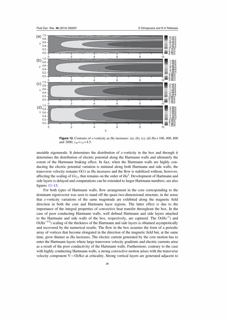
unstable eigenmode. It determines the distribution of x-vorticity in the box and through itdetermines the distribution of electric potential along the Hartmann walls and ultimately theextent of the Hartmann braking effect. In fact, when the Hartmann walls are highly con-ducting the electric potential variation is minimal along both Hartmann and side walls, thetransverse velocity remains O(1) as Ha increases and the flow is stabilized without, however,affecting the scaling of GrCr that remains on the order of Ha2. Development of Hartmann andside layers is delayed and computations can be extended to larger Hartmann numbers; see alsofigures 11–13.
For both types of Hartmann walls, flow arrangement in the core corresponding to thedominant eigenvector was seen to stand off the quasi two-dimensional structure, in the sensethat x-vorticity variations of the same magnitude are exhibited along the magnetic fielddirection in both the core and Hartmann layer regions. The latter effect is due to theimportance of the integral properties of convective heat transfer throughout the box. In thecase of poor conducting Hartmann walls, well defined Hartmann and side layers attachedto the Hartmann and side walls of the box, respectively, are captured. The O(Ha−1) andO(Ha−1/2) scaling of the thickness of the Hartmann and side layers is obtained asymptoticallyand recovered by the numerical results. The flow in the box assumes the form of a periodicarray of vortices that become elongated in the direction of the magnetic field but, at the sametime, grow thinner as Ha increases. The electric current generated by the core motion has toenter the Hartmann layers where large transverse velocity gradients and electric currents ariseas a result of the poor conductivity of the Hartmann walls. Furthermore, contrary to the casewith highly conducting Hartmann walls, a strong convective motion arises with the transversevelocity component V∼O(Ha) at criticality. Strong vortical layers are generated adjacent to
Fluid Dyn. Res. 46 (2014) 055507 D Dimopoulos and N A Pelekasis
28
Figure 12. Contours of x-vorticity as Ha increases: (a), (b), (c), (d) Ha= 100, 400, 800and 2000; cH= cS= 4.5.
the Hartmann walls where vorticity has to gradually decay to zero at the wall. Thisarrangement has to match the side layer region where vanishing electric currents exist owingto the high conductivity of the side walls. Thus corner layers, on the order of the Hartmannlayer thickness (Walker 1981), arise in order to facilitate this process, figure 11(a). Thissequence of events, i.e. vorticity generation in the core leading to large transverse velocitiesand electric currents in the Hartmann layers, followed by large x-velocities in the side layers,constitutes a ‘secondary’ motion that is analogous to the action of a hydromagnetic pumppushing fluid as a result of Lorentz forces in the Hartmann layer.
The above flow structure, especially when large discrepancies exist in the conductivitiesof the Hartmann and side walls, is quite useful in interpreting the experimental observations
Fluid Dyn. Res. 46 (2014) 055507 D Dimopoulos and N A Pelekasis
29
Figure 13. Contour plots of Ωyz on the xy plane when (a), (b), (c), (d) Ha = 100, 400,800 and 2000; cH = cS= 4.5.

by BM both in terms of the scaling at criticality but also in order to understand the onset oftime dependent secondary instability reported in the latter study. Especially as there were nocomplex eigenvalues detected in the present study, the onset of time dependent motion canonly be viewed as a secondary instability of the flow arrangement produced by the thermalinstability examined here. In this context, it should be pointed out that inertia terms in therescaled momentum balance provided by equations (3.3)–(3.5) at criticality, i.e. Gr∼Ha2, areO(1/Ha2). They drop out from the formulation in the present study since there is no motion inthe base flow, =u 00 . However, as soon as thermal instability sets in, especially when poorconducting Hartmann walls are considered, strong convective effects arise with O(Ha)transverse, V, and spanwise, W, velocity components determining the strength of the circu-latory motion in the core of the box. Consequently, right after criticality y momentum con-tains inertia terms like ∂ ∂Ha V V y(1 )2 that become O(1). As a result inertia effects may beequally important with buoyancy that drives the thermal instability and should be consideredin studying secondary instabilities and transition to turbulence.
To this end, the stability of interacting vortices, in the presence of vortical layers attachedto the walls, was investigated by Dimopoulos and Pelekasis (2012) and was seen to rapidlylose stability via a time-dependent hydrodynamic process. The associated mechanism wasmainly attributed to an elliptic instability (Tsai and Widnall 1976, Fukumoto and Hir-ota 2008) as a result of the strength and eccentricity of the interacting vortices or, as Haincreases and the strength of the wall vortical layers increases, to a shear layer instability.Thermal interaction between nearby vortices that carry hot rising fluid was examined byGershuni and Zhukovitskii (1982) in the context of the two-layer Rayleigh–Bénard problem,who also showed that standing or traveling wave instabilities may arise, depending on therelative arrangement of the vortices. All the above elements are present in the flowarrangement that arises at criticality in the present study and they are expected to play a role inthe post-critical regime as Gr increases for fixed Hartmann. Furthermore, as the aboveinstabilities introduce three dimensionality to the system, the validity of the assumption ofquasi two dimensionality of the flow needs to be reexamined as well as its role in thetransition to turbulence, when strong magnetic fields are present. A full nonlinear analysis is,of course, necessary in order to assess the relative importance of the effects discussed above,as well as the relevance of secondary hydrodynamic instabilities in establishing a flowarrangement that will conform with the quasi 2D structure.
Acknowledgement
This work was performed in the framework of the EURATOM-Hellenic Republic Associa-tion and is supported by the European Union within the Fusion Program. Use of the super-computing facilities at HELIOS in part of the simulations performed, is acknowledged.
References
Blackford L S et al 1997 ScaLAPACK Users Guide (Philadelphia: SIAM)Buhler L 1996 Instabilities in quasi-two dimensional magnetohydrodynamic flows J. Fluid Mech. 326
125–50Buhler L 1998 Laminar buoyant magnetohydrodynamic flow in vertical rectangular ducts Phys. Fluids
10 223–36Buhler L and Mistrangelo C 2010 MHD mock-up experiments for studying pressure distribution in a
helium-cooled liquid-metal blanket IEEE Tran. Pl. Sci. 38 254–8
Fluid Dyn. Res. 46 (2014) 055507 D Dimopoulos and N A Pelekasis
30
Buhler L and Norajitra B 2003 Magnetohydrodynamic flow in the dual coolant blanketKernforschungszentrum Karlsruhe Technical Report KfK 6802 pp 1–21
Burr U and Muller U 2002 Rayleigh–Bénard convection in liquid metal layers under the influence of ahorizontal magnetic field J. Fluid Mech. 453 345–69
Chandrasekhar S 1961 Hydrodynamic and Hydromagnetic Stability (Oxford: Oxford Clarendon Press)Cliffe K A, Garratt T J and Spence A 1993 Eigenvalues of the discretized Navier–Stokes equation with
application to the detection of Hopf bifurcations Adv. Comput. Mathematics 1 337–56Davidson P A 2001 An Introduction to Magnetohydrodynamics (Cambridge: Cambridge Univer-
sity Press)Davoust L, Cowley M D, Moreau R and Bolcato R 1999 Buoyancy-driven convection with a uniform
magnetic field: part 2. Experimental investigation J. Fluid Mech. 400 59–90Dimopoulos D and Pelekasis N 2012 Three dimensional stability of free convection vortices in the
presence of a magnetic field Fluid Dyn. Res. 44 031405Fukumoto Y and Hirota M 2008 Elliptical instability of a vortex tube and drift current induced by it
Phys. Scr. T132 014041Gelfgat A Y and Molokov S 2011 Quasi two dimensional convection in a three dimensional laterally
heated box in a strong magnetic field normal to main circulation Phys. Fluids 23 034101Gershuni G Z and Zhukovitskii E M 1982 Monotonic and oscillatory instabilities of a two layer system
of immiscible fluids when heated from below Sov. Phys. Dokl. 27 531–3Kharitsa A, Molokov A, Aleksandrova A and Buhler L 2004 Buoyant convection in the HCLL blanket
in a strong, uniform magnetic field Kernforschungszentrum Karlsruhe Technical Report KfK 6959pp 1–127
Lyubimov D V, Lyubimova T P, Perminov A B, Henry D and Ben Hadid H 2009 Stability ofconvection in a horizontal channel subjected to a longitudinal temperature gradient. Part 2. Effect of amagnetic field J. Fluid Mech. 635 297–319
Pelekasis N 2006 Bifurcation diagrams, linear stability analysis and dynamic simulations of freeconvection in a differentially heated cavity in the presence of a magnetic field Phys. Fluids18 034101
Planas R, Badia S and Codina R 2011 Approximation of the inductionless MHD problem using astabilized finite element method J. Comp. Phys. 230 2977–96
Pothérat A, Sommeria J and Moreau R 2000 An effective two-dimensional model for MHD flows withtransverse magnetic field J. Fluid Mech. 424 75–100
Pothérat A, Sommeria J and Moreau R 2005 Numerical simulations of an effective two-dimensionalmodel for flows with a transverse magnetic field J. Fluid Mech. 534 115–43
Reid W H and Harris D L 1958 Some further results on the Bénard problem Phys. Fluids 1 102–10Saad Y 2003 Iterative Methods for Sparse Linear Systems 2nd edn (Philadelphia: SIAM)Smolentsev S, Moreau R and Abdou M 2008 Characterization of key magnetohydrodynamic
phenomena in PbLi flows for the US DCLL blanket Fusion Engin. and Design 83 771–83Smolentsev S, Moreau R, Buhler L and Mistrangelo C 2010 MHD thermofluid issues of liquid-metal
blankets: phenomena and advances Fusion Engin. and Design 85 1196–205Smolentsev S, Vetcha N and Moreau R 2012 Study of instabilities and transitions for a family of quasi-
two-dimensional magnetohydrodynamic flows based on a parametrical model Phys. Fluids24 024101
Sommeria J and Moreau R 1982 Why, how and when MHD turbulence becomes two-dimensionalJ. Fluid Mech. 118 507–18
Takashima M 1994 The stability of natural convection in a vertical layer of electrically conducting fluidin the presence of a transverse magnetic field Fluid Dyn. Res. 14 121–34
Tsai C and Widnall S E 1976 The stability of short-waves on a straight vortex filament in a weakexternally imposed strain field J. Fluid Mech. 73 721–33
Vetcha N, Smolentsev S, Abdou M and Moreau R 2013 Study of instabilities and transitions for afamily of quasi-two-dimensional magnetohydrodynamic flows based on a parametric model Phys.Fluids 25 024102
Walker J S 1981 Magnetohydrodynamic flows in rectangular ducts with thin conducting walls—part IJ. Mecanique 20 79–112
Fluid Dyn. Res. 46 (2014) 055507 D Dimopoulos and N A Pelekasis
31


![Triple- diffusive convection in a micropolar ferrofluid in ... · layer. The thermal convection in Newtonian ferro fluid has been studied by many authors [16-25]. Rayleigh-Bénard](https://img.pdfslide.us/doc/110x75/5fba48033566f3202e54da1b/triple-diffusive-convection-in-a-micropolar-ferrofluid-in-layer-the-thermal.jpg)