3D SKELETON CONSTRUCTION FROM MULTIPLE CAMERA

VIEWS FOR QUANTIFYING GAIT PARAMETERS

by

Saket Gupta

A thesis submitted in fulfillment of the requirements for the degree of

Master of Science in Computer Science

The University of Texas At Arlington

May 2020

1

Copyright © by Saket Gupta 2020

All Rights Reserved

1 | P a g e

"THE UNIVERSITY OF TEXAS AT ARLINGTON"

ABSTRACT

3D Skeleton Construction from Multiple Camera Views for Quantifying Gait

Parameters

by Saket Gupta

Chairperson of the Supervisory Committee: Professor Manfred Huber Department of CSE

Research has shown that human gait characteristics permit inference with respect

to different personal and health characteristics and can thus be used as a

diagnostic tool. To do this automatically it is important to be able to extract them

from senor information. This thesis work is aimed at doing this from multiple

camera views and for this focuses on construction of a 3D body skeleton from

multiple viewpoint video (MVV) and then quantifying a number of gait

characteristics such as swing time, step time, cadence, stride length, single

support, or double support.

The method introduced here uses a marker-less approach over marker-based

approach for skeleton extraction because it significantly reduces preparation time

as well as the equipment cost compared to marker-based techniques. The

drawback with the marker-less approach is that the processing time is longer

because a body model needs to be created. The solution proposed in this thesis

attempts to reduce the processing time by using transfer learning utilizing pre-

trained deep learning models and then solving inverse projection problem to get

the 3D body skeleton.

The extracted visual and 3D skeleton data, along with IMU data from different

parts of body is then analyzed to quantify gait characteristics. In particular, three

2 | P a g e

Neural Networks were developed and trained to quantify gait characteristics of

human body, one each for sensors data, 2D visual body data and 3D body

skeleton data. These Neural Networks were trained to classify whether the

human body is in a Single support (left leg), Single support (right leg) or Double

support phase. The performance of the networks were evaluated against ground

truth and the performance based on the different sensor sets were compared.

Among the three Neural Networks the classification accuracy using IMU data

was better than using both 2D and 3D skeleton data. Among the visually derived

models, the accuracy using 3D skeleton data was better than for 2D visual data.

In addition, gait characteristics like Gait Velocity, Step time, Stride length, Stride

time, Swing time were extracted from the 3D body skeleton and the performance

was validated for multiple individuals.

3 | P a g e

ACKNOWLEDGMENTS

The author wishes to express sincere appreciation to the mentor Professor Manfred Huber for the continuous support and motivation during all the time of research and writing of this thesis.

Discussions and reviews made by my mentor on the regular basis kept me spirited and helped me work to my full capacity. I am also grateful for his Insightful guidance especially at the critical stages of the thesis.

It has been my privilege of the lifetime to work under the guidance of Dr. Manfred Huber.

I deem it my duty to mention that the research work was hugely facilitated by the resources provided in the Laboratory.

I would like to extend my gratitude to my committee members Dr. Shirin Nilizadeh and Dr. Ming Li for providing me insightful suggestions and valuable feedback.

I cannot be grateful enough to my mother and father, especially my mother who devoted her life to make me the person I am today.

TABLE OF CONTENTS

List of Tables .............................................................................................................................................................. 6 List of Figures ............................................................................................................................................................. 7 Glossary ....................................................................................................................................................................... 8 Chapter I: Introduction ............................................................................................................................................ 9

Introduction and Background .......................................................................................................................... 9 Related Work .................................................................................................................................................... 10 Proposed Solution and Contribution ........................................................................................................... 12 Data Used for Thesis ...................................................................................................................................... 13

Chapter II: Extracting information from Videos ............................................................................................. 14 Identifying the critical points ......................................................................................................................... 14

Chapter III: 2D Skeleton Extraction using Transfer Learning ...................................................................... 17 Pretrained Models ........................................................................................................................................... 17 Human Pose NN ..................................................................................................................................... 18 Human 3.6M ............................................................................................................................................ 18 Selecting Pretrained Model for Transfer Learning .................................................................................... 19 Neural Network Architecture Used for 2D Skeleton Extraction .......................................................... 19 Dealing with Edge Cases ................................................................................................................................ 20 Preprocessing for Transfer Learning ........................................................................................................... 21 Extracting Frames from Video ............................................................................................................. 21 Extracting the Background Per Camera .............................................................................................. 22 Extracting Silhouette Frames ................................................................................................................ 23 Cropping smallest square encompassing the body............................................................................ 23 Resizing the square .................................................................................................................................. 24 Predictions of Body Joints ..................................................................................................................... 25 Creating a body skeleton ........................................................................................................................ 27 Projecting predicted body joints to original image ............................................................................ 29

Chapter IV: The 3D skeleton ............................................................................................................................... 30 Camera Matrix .................................................................................................................................................. 30 Triangulation..................................................................................................................................................... 31 Eliminating the outliers .................................................................................................................................. 32 Minimizing the Mean Square Error ............................................................................................................. 32 Using SVD to solve the Mean Square Error .............................................................................................. 32 Transformation matrices to convert from 2D to 3D ............................................................................... 34

Chapter V: Extracting Details About Body Stride ........................................................................................... 39 Classification ..................................................................................................................................................... 39 Classifying walking state from sensors data ................................................................................................ 41 Classifying walking state from visual (2D) Data ........................................................................................ 42 Classifying walking state from visual (3D) Data ........................................................................................ 45 Calculating Swing Time .................................................................................................................................. 47 Calculating time to complete stride .............................................................................................................. 47 Calculating stride length ................................................................................................................................. 47 Calculating Cadence ........................................................................................................................................ 48

5 | P a g e

Calculating gait velocity .................................................................................................................................. 48 Web Application .............................................................................................................................................. 48

Chapter VI: Conclusion ........................................................................................................................................ 50 Bibliography ............................................................................................................................................................. 52 Data Set References ................................................................................................................................................ 53

6 | P a g e

LIST OF TABLES

Number ..................................... Page 1. Number of Frames Capturing Human Per Camera .................................................................................... 21

2. Probability (*100) of correct Estimation ........................................................................................................ 26

3. Summary Neural Network for sensors data .................................................................................................. 41

4. Summary Neural Network for 2D data ......................................................................................................... 43

5. Summary Neural Network for 2D data ......................................................................................................... 45

7 | P a g e

LIST OF FIGURES

Number ..................................................................................................................................................................... Page 1. Body Joints Needed to Estimate skeleton ........................................................................................... 14

2. Average Error distance – MPII + LSP validation set ....................................................................... 18

3. Average Error distance – Human 3.6m validation set ...................................................................... 19

4. Inception Res Net v2 ............................................................................................................................... 20

5. Human body not inside camera's field of view .................................................................................. 21

6. Extracted Frame from video of camera one ....................................................................................... 22

7. Extracted Background from camera two ............................................................................................. 22

8. Extracted Silhouette from video of camera one ................................................................................. 23

9. Cropped Square Image ............................................................................................................................ 24

10. Body Joints Predicted by Neural Network .......................................................................................... 25

11. Camera Configuration of the Total Capture Dataset ....................................................................... 26

12. Average Probability of Correct Prediction for each of 8 Cameras ................................................ 27

13. Joining Body Joints to make a skeleton ................................................................................................ 28

14. Projecting the extracted body points into the original image .......................................................... 29

15. Triangulation ............................................................................................................................................. 32

16. Camera Coordinate to Image Coordinate System .............................................................................. 34

17. Image Coordinate System to World Coordinate System .................................................................. 35

18. 3D skeleton ................................................................................................................................................ 37

19. Single Support (Left Leg), Single Support (Right Leg), Double Support ...................................... 40

20. Model Loss from sensors data ............................................................................................................... 42

21. Model Accuracy from sensors data ....................................................................................................... 42

22. Model Loss from 2D data ....................................................................................................................... 44

23. Model Accuracy from 2D data .............................................................................................................. 44

24. 3D Model of Left, Right Leg in motion, Standing still ..................................................................... 46

25. Model Loss from 3D data ....................................................................................................................... 46

26. Model Accuracy from 3D data .............................................................................................................. 47

27. Application displaying video and its Gait Analysis ............................................................................ 49

8 | P a g e

GLOSSARY

Cadence is the number of steps taken in a given time, usually steps per minute

Double support the time over which the body is supported by both legs

Gait Analysis is the systematic study of locomotion, more specifically the study of animal or human

motion, using the eye and the brain of observers, augmented by instrumentation for measuring body

movements, body mechanics, and the activity of the muscles.

Gait velocity (Average) the stride length divided by the stride time.

Kinematics is a subfield of classical mechanics that describes the motion of points, bodies, and

systems of bodies without considering the forces that cause them to move. Kinematics, as a field of

study, is often referred to as the "geometry of motion" and is occasionally seen as a branch of

mathematics.

Projection Matrix a camera matrix or (camera) projection matrix is a matrix which describes

the mapping of a pinhole camera from 3D points in the world to 2D points in an image.

Silhouette cast or show (someone or something) as a dark shape and outline against a lighter

background.

Single support the time over which the body is supported by only one leg

Step time the time between two consecutive heel strikes

Stride Length is defined as the distance between successive ground contacts of the same foot

Stride time the time between two consecutive heel strikes by the same leg, one complete gait cycle

Swing time the time taken for the leg to swing through while the body is in single support on the

other leg

Total support the total time a foot is in contact with the ground during one complete gait cycle.

Transfer learning is a research problem in machine learning that focuses on storing knowledge

gained while solving one problem and applying it to a different but related problem.

Triangulation refers to the process of determining a point in 3D space given its projections onto two,

or more, images.

9 | P a g e

C h a p t e r 1

INTRODUCTION

Introduction and Background:

Gait analysis is the systematic study of human motion for measuring body movements, body

mechanics and activity of muscles and can provide significant amounts of useful information about an

individual in terms of their behavior but also in terms of health status, potential physical or mental

issues, injuries, or overall fitness and capability status. With the advent of increasing amounts of data

related to human motion either in lab environments or from real-time sensors, this has led to a drive

to investigate automatic gait analysis from both video and wearable sensor data.

Surging availability of data with the increase in the use of smart watches, mobiles, and cameras has

attracted broad attention from both academia and industry. Most smartwatches and mobiles contain

three sensors – Accelerometer, Magnetometer and Gyroscope. This data is useful to analyze the body

pose and facilitate gait analysis. Various other types of man-made sensors as described by Tao[11],

have also been used to analyze gait characteristics. Generally, these can be divided into wearable

sensors that provide data regarding the body dynamics and are carried on the body, and

external/environmental sensors, such as cameras, 3D vision sensors, or sensor systems that measure

the distortion of an electromagnetic field, which observe human motion within a specific environment.

The work in this thesis focuses mainly on motion analysis from multiple cameras but also performs

limited comparison with data obtained from wearable sensors. The advantage of gait analysis from

cameras is that cameras are easy to deploy in an environment and do not require any action to be taken

by the individual. This makes them ideal for situations such as health monitoring for elderly persons or

persons with dementia where the reliable wearing and charging of wearable sensors would be too

cumbersome. The main disadvantage is that camera-based systems can only cover a limited area while

wearable sensors move with the individual and can thus be used in any place the person moves to.

In this thesis, the focus is on the construction of a 3D skeleton model of the individual from multiple

2D camera views and the subsequent learning of gait analysis models that can extract important gait

10 | P a g e

parameters from the resulting data. We have used pre-trained models on datasets like Human3.6M by

Catalin[8], Max Planck Institute’s MPII Dataset [5] and Leeds Sports Pose Dataset [6] to estimate the

body skeleton on the Total Capture Dataset by Gilbert[9]. The gait characteristics of the subject were

extracted from these body skeletons.

To achieve this, 2D body skeleton data is extracted for each camera video stream. These 2D body

skeletons data are then fused together to generate the 3D body skeleton data.

Based on the extracted 3D skeleton, spatial-temporal gait features like single support (left leg or right

leg) or double support, were estimated with more than 98% accuracy. For this, we have developed

three Neural Networks to quantify gait characteristics of human body. The outputs of the neural

networks were evaluated against ground truth. Comparing the information from three Neural

Networks that use either a large array of wearable sensors, 2D video, or the extracted 3D skeleton, the

classification accuracy of sensors neural network was better than neural networks for both 2D and 3D.

The classification accuracy of neural network for 3D was better than the neural network for 2D.

In addition to these characteristics, gait features like Cadence, number of steps taken, swing time,

stride time were also accurately estimated base on the extracted information from the 3D skeleton.

Related Work:

The problem of body pose estimation approaches can be split into two broad categories; one is a top-

down approach, which is to fit an articulated limb kinematic model to the source data, and the other

approach is a bottom up approach which is purely data driven.

Huttenlocher[12] provides a top down approach where a body model is provided. The SMPL body

model by Loper[6] has been widely used in the top down approach. Later Marcard[12] used IMU data

with the SMPL body model, yielding body pose estimates without visual data. Huang[2] uses a 3D

shape matching algorithm to classify between different body poses. In another paper Marcard[5] uses a

realistic body model that incorporates anthropomorphic constraints (with a skeletal rig) along with

sparse IMU data to predict full body pose.

11 | P a g e

Placing multiple sensors on the body is intrusive and uncomfortable and therefore has not been widely

used, so big dataset have not been collected. Furthermore, a problem with Marcard’s approach is that

errors are accumulated over time as forward kinematic solving is performed on the IMU data to get

the final pose. Apart from that a bad initial guess of the body model can further aggravate the error in

the estimated body pose.

In a bottom up approach, Sanzari [4] estimates the location of 2D joints before predicting 3D pose

using appearance and probable 3-D pose of the discovered parts with a hierarchical Bayesian model.

The hierarchical model has two levels. The first level builds a dictionary of 3D human poses, while the

second level provides corresponding images from a number of view points. The Limitation of this

model is that the dictionary has a set of predefined outputs; therefore at times it can be a bit removed

from the actual data.

The visual approach to estimate 3D pose can be broadly categorized in two categories, the marker-

based approach and the marker-less approach.

The marker-based approach uses image data to track markers and measures their orientation to the

camera. But there are a few drawbacks such as a high cost as well as significant time overhead that is

incurred due to the need for a special suit and IR cameras, and the requirement to wear this special

suit. Another issue is that the relative position of underlying bone to the initial marker location does

often not remain stable, leading to skin artifacts. Attached markers themselves also often influence the

actor’s movement. Though Microsensors are expected to play an increasingly important role here

(Zeng[10]) and could reduce these effects,

The marker-less approach significantly reduces the actor’s preparation time as well as the equipment

cost compared to marker-based. But in this approach the processing time is longer because a model

needs to be created. The solution proposed in this thesis attempts to reduce the processing time by

using a deep learning model trained on a simpler dataset and transferring it to the more complex multi-

view problem.

For the marker-less approach several methods to reconstruct the outer surface of the body were

proposed by Corazza[14]. Using the outer surface, Phantom volumes are derived. These Phantom

12 | P a g e

volumes deviate from the ground truth. The solution proposed in this thesis directly derives the body

skeleton instead of Phantom volumes.

Zhou[3] uses monocular images with an image driven 2D part detector along with 3D geometric pose

prior to estimate 3D pose. Helten [15] used a single depth camera with IMUs to estimate the body

pose. Bregler[16] utilizes only 2D information to estimate body pose, but biomechanical applications

require a 3D model. Hao[7] uses high order constraints to anchor multiple body parts simultaneously,

and utilizes an efficient linear relaxation method to solve the consistent max-covering problem. In the

marker-less approach, solving for 3D body pose from visual data is an under-constrained problem as it

has a large number of degrees of freedom. Increasing the number of cameras capturing the body helps

to resolve this problem. The estimation of 3D body pose from multiple viewpoint video (MVV) is a

less explored area. This thesis is an attempt to explore this area.

Proposed Solution and Contribution:

To extract the 3D body skeleton data from multi-view video, we propose to estimate 2D body

skeleton data in each of the camera views and then solve for the inverse projection problem, to fuse

2D body skeletons together and generate the 3D body skeleton data. The 2D body skeleton could be

estimated using a marker-less or marker-based approach. Though the dataset we are using has body

markers available, we propose to use a marker-less approach rather than the marker based approach to

obtain the 2D body skeleton because the marker-less approach seems more applicable to real world

data, especially in health and diagnosis settins as it significantly reduces the actor’s preparation time as

well as the equipment cost compared to the marker-based approach. The drawback with the marker-

less approach is that the processing time is longer because a body model needs to be created. The

solution proposed in this thesis attempts to reduce the processing time by using pre-trained deep

learning models. We use pretrained models to estimate 2D body skeletons on Human3.6M, Max

Planck Institute’s MPII Dataset and Leeds Sports Pose Dataset.

The solution proposed in this thesis uses triangulation to obtain 3D body skeleton information instead

of extracting Phantom volumes because it has less deviation from the ground truth. Also, minimizing

the error is easier for body skeleton data as compared to phantom volumes. As we need to solve for

13 | P a g e

minimize 1/n ∑ (A-B)2

where A is set of estimated points and B is set of corresponding ground truth

The sets A and B are smaller for a body skeleton compared to phantom volumes. Further, we do not

require to extract the 3D Hull to estimate the gait characteristics.

The proposed approach has an advantage over the model-based approach, e.g. by Marcard [12], in that

the errors are not accumulated over time as there is no need to do matching (with a body model) for

every frame. Thus, the results with this approach should be more robust.

Further we propose three Neural Networks to quantify gait characteristics of the human body, one

each for wearable sensor data, 2D body skeleton data, and 3D body skeleton data. These Neural

Networks classify whether the human body is in Single support (left leg), Single support (right leg) or

in Double support.

Data used for the thesis:

The TotalCapture[3] dataset is a dataset containing marker-based multi-camera capture. Though in

our proposed solution we are not using the marker data. It is the first dataset to have fully

synchronized multi-view video, IMU and Vicon labelling for a large number of frames (∼1.9 Million),

for many subjects, activities and viewpoints. We are using the walking subpart of the dataset. The

dataset contains a number of subjects performing varied actions and viewpoints. It was captured

indoors in a volume measuring roughly 8x4m with 8 calibrated HD video cameras at 60Hz. There are

4 male and 1 female subjects, each performing four diverse performances, repeated 3 times: ROM,

Walking, Acting and Freestyle. There are a total of 1892176 frames of synchronized video, IMU and

Vicon data (although some is withheld as test footage for unseen subjects). The variation and body

motions contained in particular within the acting and freestyle sequences are very challenging with

actions such as yoga, giving directions, bending over and crawling performed in both the train and test

data. We are using the part of data where the subjects are walking. These constitute around 350,000

frames out of around 1,800,000 frames of the total dataset.

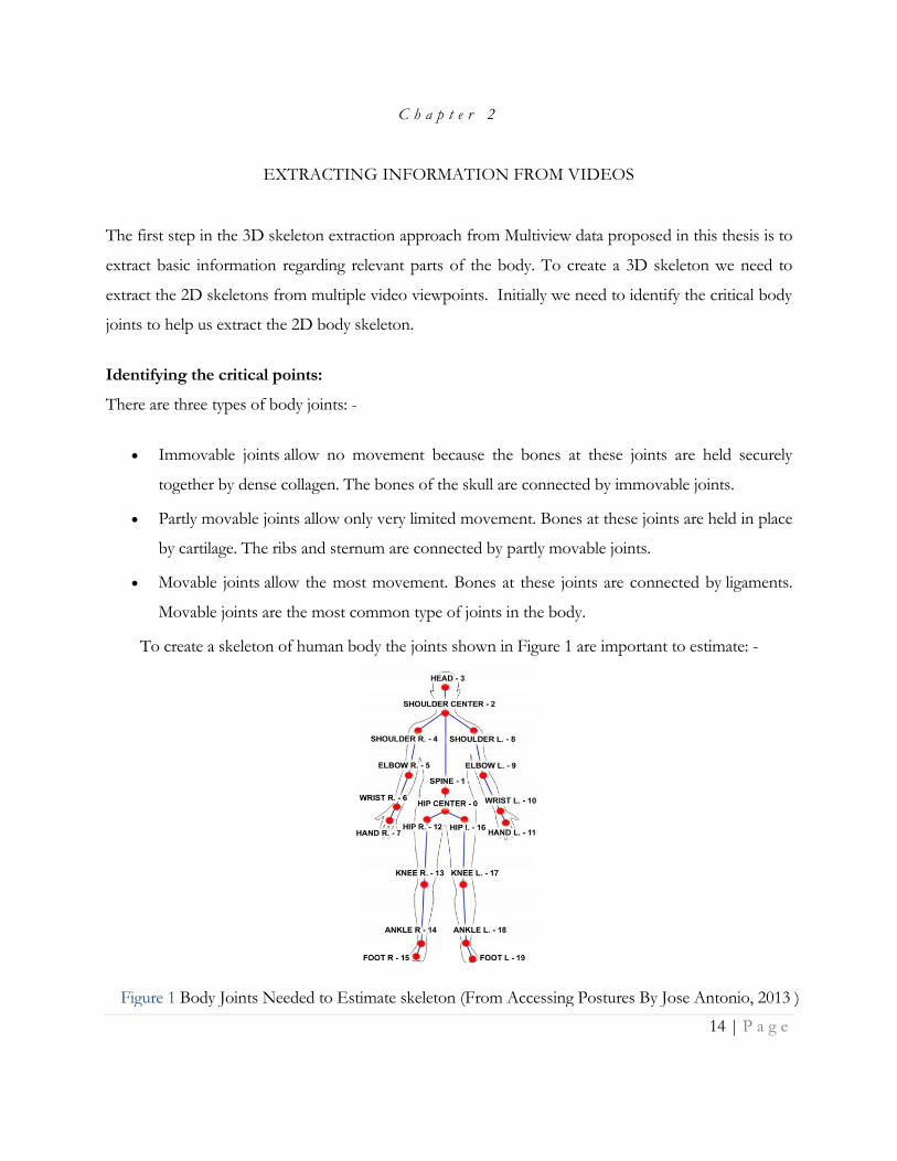
14 | P a g e

Figure 1 Body Joints Needed to Estimate skeleton (From Accessing Postures By Jose Antonio, 2013 )

C h a p t e r 2

EXTRACTING INFORMATION FROM VIDEOS

The first step in the 3D skeleton extraction approach from Multiview data proposed in this thesis is to

extract basic information regarding relevant parts of the body. To create a 3D skeleton we need to

extract the 2D skeletons from multiple video viewpoints. Initially we need to identify the critical body

joints to help us extract the 2D body skeleton.

Identifying the critical points:

There are three types of body joints: -

• Immovable joints allow no movement because the bones at these joints are held securely

together by dense collagen. The bones of the skull are connected by immovable joints.

• Partly movable joints allow only very limited movement. Bones at these joints are held in place

by cartilage. The ribs and sternum are connected by partly movable joints.

• Movable joints allow the most movement. Bones at these joints are connected by ligaments.

Movable joints are the most common type of joints in the body.

To create a skeleton of human body the joints shown in Figure 1 are important to estimate: -

15 | P a g e

We need to keep track of the movable joints more rigorously compared to immovable or partially

movable joints like skull, thorax because the immovable and partially immovable body joints are more

constrained

The set of movable joints which are very important to track the body skeleton include, e.g. ankle, knee,

hip, shoulder, elbow, and wrist because these joints change their position at a faster rate compared to

other body joints.

Transfer learning was used to extract these critical body joints.as we will see in the next chapter.

In Transfer learning we use pretrained models to get results for our dataset. There are two pre-trained

models available which are relevant for our dataset. These two pretrained models :-

1. Max Planck Institute’s MPII Dataset and Leeds Sports Pose Dataset (Pretrained model

MPII+ LSP)

2. Human3.6M pretrained model.

Both these pretrained models estimate the following body joints :-

1.Right ankle

2. Right knee

3.Right hip

4.Left hip

5.Left knee

6. Left ankle

7.Pelvis

8.Thorax

16 | P a g e

9.Upper neck

10.Head top

11.Right wrist

12.Right elbow

13.Right shoulder

14.Left shoulder

15.Left elbow

16.Left wrist

Estimation of the above body joints is sufficient to construct a body skeleton. In the next chapter we

will discuss extraction of the 2D skeleton from marker-less video data using transfer learning.

17 | P a g e

C h a p t e r 3

2D SKELETON EXTRACTION USING TRANSFER LEARNING

Transfer Learning makes use of the knowledge gained while solving one problem and applying it to a

different but related problem. When we train the network on a large dataset, we train all the

parameters of the neural network and therefore the model is learned. It may take hours on your GPU.

If the new dataset is similar, the same weights which were learned can be used for extracting the

features from the new dataset.

In the approach presented here this is used to overcome the issue that the multi-view dataset does not

contain ground truth information for the body part extraction. Also, the TotalCapture dataset used for

multi-view skeleton construction contains images with the human in very different locations within the

image frame, making learning of body part extraction more complex. Instead of learning the extraction

from this dataset, we thus opt to utilize a model trained on a more specialized dataset for 2D body

extraction and then transfer the resulting pre-trained model to skeleton extraction on the TotalCapture

dataset.

Pretrained Models

A pre-trained model is a model created to solve a problem, in our case in the form of a neural network

(NN). After the training of the network with a dataset and loss function for that problem, the weights

are learned. The learned weights of the network can subsequently be used to solve similar problem.

Now, instead of building a model from scratch we can use the pretrained model to solve our problem.

Pretrained models are more useful when their training was done on a large dataset and the problem

being solved is similar to the problem on which the pretrained model was initially trained. In the work

presented in this thesis, a pretrained model for body segment identification is used to be subsequently

transferred to the TotalCapture dataset and the skeleton extraction problem.

A number of specialized, labeled datasets for body segment identification exist and can be used to

pretrain a neural network model.

18 | P a g e

Human Pose NN

The checkpoint MPII+LSP.ckpt model for visual joint extraction from images [1] was trained on

images from the MPII and LSP database. In the graph in Figure 2 you can see the average distance

between predicted and desired joints on a validation set of about 6 000 images.

Figure 2 Average Error distance - MPII + LSP validation set (Ref: http://human-pose.mpi-inf.mpg.de/)

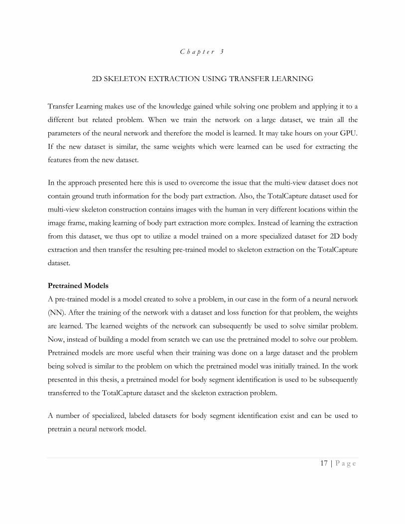
Human 3.6M (action walking)

The checkpoint Human3.6m.ckpt model [2] was trained on the database Human 3.6m and only on

the walking components of all individuals’ 48 sequences. Person S5 (8 sequences) was used for

validation purposes and the average distance between predicted and desired joints is shown in Figure

3. Errors in this model are smaller compared to the one trained on MPII+LSP. The reason is that

Human 3.6m sequences are very monotonous and thus human pose estimation is less challenging.

However, this also means that the diversity in the dataset is lower and thus the model might be less

robust.

19 | P a g e

Figure 3 Average error distance - Human 3.6m validation set (Ref: http://vision.imar.ro/human3.6m/description.php)

Selecting the Model for Transfer Learning

We chose the model pretrained on MPII+LSP instead of the one on Human3.6M to obtain the 2D

skeleton of the person for the TotalCapture dataset. We choose the MPII+LSP pretrained model over

the Human3.6M pretrained model even though the reported error on their respective datasets is

smaller using the Human3.6M pretrained model because the sequences in the Human3.6M model are

very monotonous, and using it on the TotalCapture dataset will produce more error compared to the

MPII+LSP pretrained model since the diversity of motions and viewing angles in the TotalCapture

dataset is significantly higher than in the Human3.6M dataset and thus the MPII+LSP dataset

contained a more reflective distribution of body views for the multi-view skeleton extraction problem.

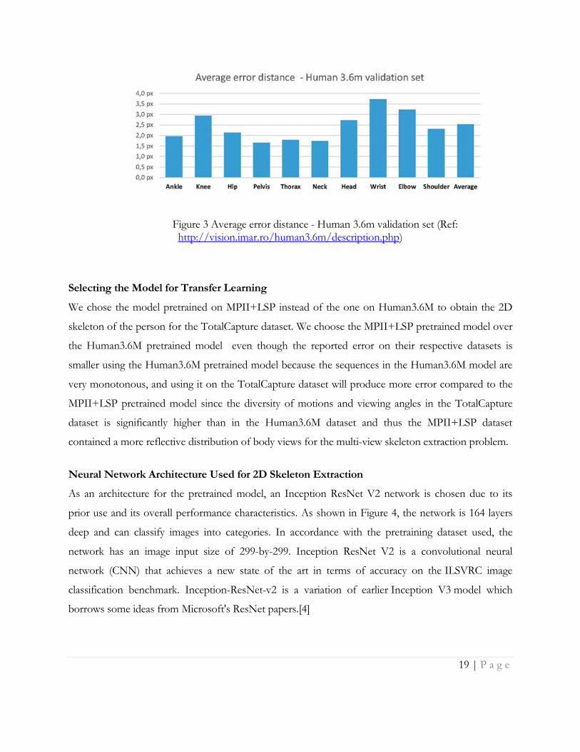
Neural Network Architecture Used for 2D Skeleton Extraction

As an architecture for the pretrained model, an Inception ResNet V2 network is chosen due to its

prior use and its overall performance characteristics. As shown in Figure 4, the network is 164 layers

deep and can classify images into categories. In accordance with the pretraining dataset used, the

network has an image input size of 299-by-299. Inception ResNet V2 is a convolutional neural

network (CNN) that achieves a new state of the art in terms of accuracy on the ILSVRC image

classification benchmark. Inception-ResNet-v2 is a variation of earlier Inception V3 model which

borrows some ideas from Microsoft's ResNet papers.[4]

20 | P a g e

Figure 4 Inception ResNet V2 (Ref: https://ai.googleblog.com/)

Dealing with edge cases

The TotalCapture dataset was recorded within a fixed volume using stationary cameras in different

locations. As opposed to the pretraining datasets, no division of images or labeling with respect to

whether the person is visible in the particular view and where the person is has been performed. As a

consequence, there are certain cases where a very small part or none of the human body is in field of

view of a camera, e.g. Figure 5. We need to remove those frames from our pipeline. To remove those

special cases we have taken a threshold of 100 pixels i.e. if the maximum of X and Y lengths of the

human body captured inside the frame is less than 100 pixels we do not use that frame to apply

transfer learning. The 2d pose estimation for that frame will not help to improve accuracy for creating

the 3D pose. Though as we have 8 cameras, this problem is mitigated because most probably other

cameras would have captured the human body for that timestamp. Table 1 shows the number of valid

frames from each of the 8 cameras for a representative video sequence of length 61 seconds (3671

frames) illustrating the variation of visibility across different viewpoints.

21 | P a g e

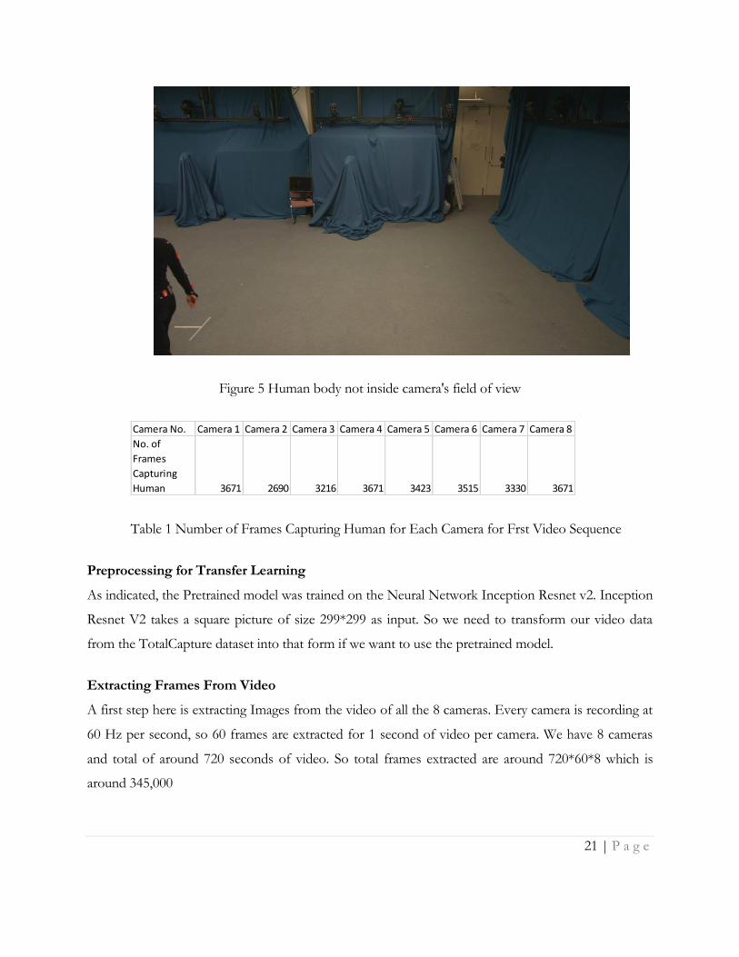
Figure 5 Human body not inside camera's field of view

Table 1 Number of Frames Capturing Human for Each Camera for Frst Video Sequence

Preprocessing for Transfer Learning

As indicated, the Pretrained model was trained on the Neural Network Inception Resnet v2. Inception

Resnet V2 takes a square picture of size 299*299 as input. So we need to transform our video data

from the TotalCapture dataset into that form if we want to use the pretrained model.

Extracting Frames From Video

A first step here is extracting Images from the video of all the 8 cameras. Every camera is recording at

60 Hz per second, so 60 frames are extracted for 1 second of video per camera. We have 8 cameras

and total of around 720 seconds of video. So total frames extracted are around 720*60*8 which is

around 345,000

Camera No. Camera 1 Camera 2 Camera 3 Camera 4 Camera 5 Camera 6 Camera 7 Camera 8

No. of

Frames

Capturing

Human 3671 2690 3216 3671 3423 3515 3330 3671

22 | P a g e

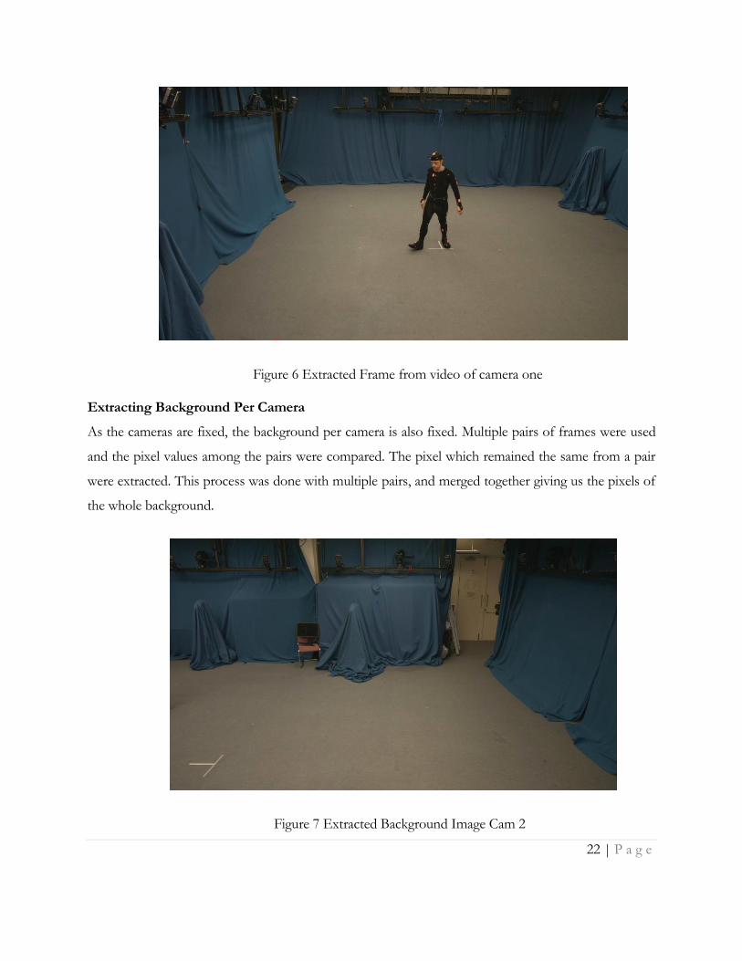
Figure 6 Extracted Frame from video of camera one

Extracting Background Per Camera

As the cameras are fixed, the background per camera is also fixed. Multiple pairs of frames were used

and the pixel values among the pairs were compared. The pixel which remained the same from a pair

were extracted. This process was done with multiple pairs, and merged together giving us the pixels of

the whole background.

Figure 7 Extracted Background Image Cam 2

23 | P a g e

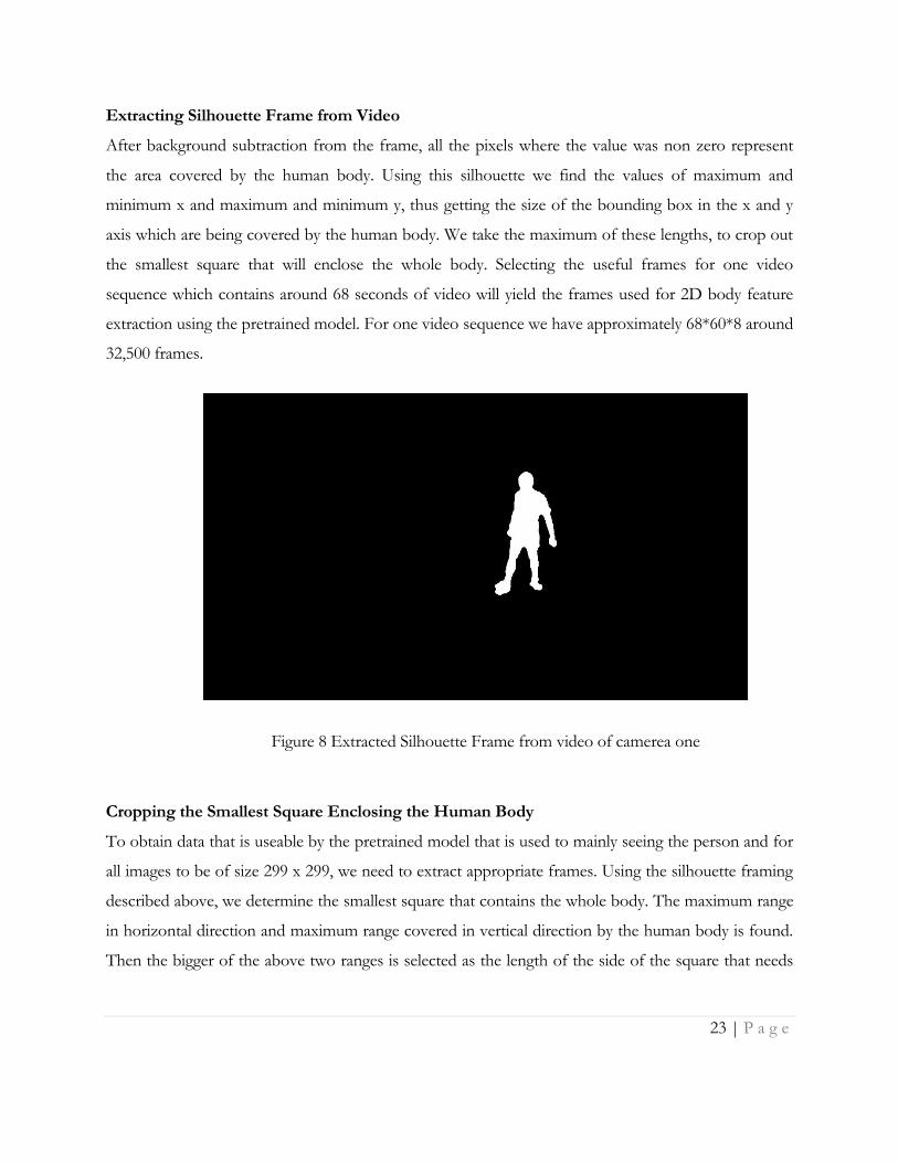
Extracting Silhouette Frame from Video

After background subtraction from the frame, all the pixels where the value was non zero represent

the area covered by the human body. Using this silhouette we find the values of maximum and

minimum x and maximum and minimum y, thus getting the size of the bounding box in the x and y

axis which are being covered by the human body. We take the maximum of these lengths, to crop out

the smallest square that will enclose the whole body. Selecting the useful frames for one video

sequence which contains around 68 seconds of video will yield the frames used for 2D body feature

extraction using the pretrained model. For one video sequence we have approximately 68*60*8 around

32,500 frames.

Figure 8 Extracted Silhouette Frame from video of camerea one

Cropping the Smallest Square Enclosing the Human Body

To obtain data that is useable by the pretrained model that is used to mainly seeing the person and for

all images to be of size 299 x 299, we need to extract appropriate frames. Using the silhouette framing

described above, we determine the smallest square that contains the whole body. The maximum range

in horizontal direction and maximum range covered in vertical direction by the human body is found.

Then the bigger of the above two ranges is selected as the length of the side of the square that needs

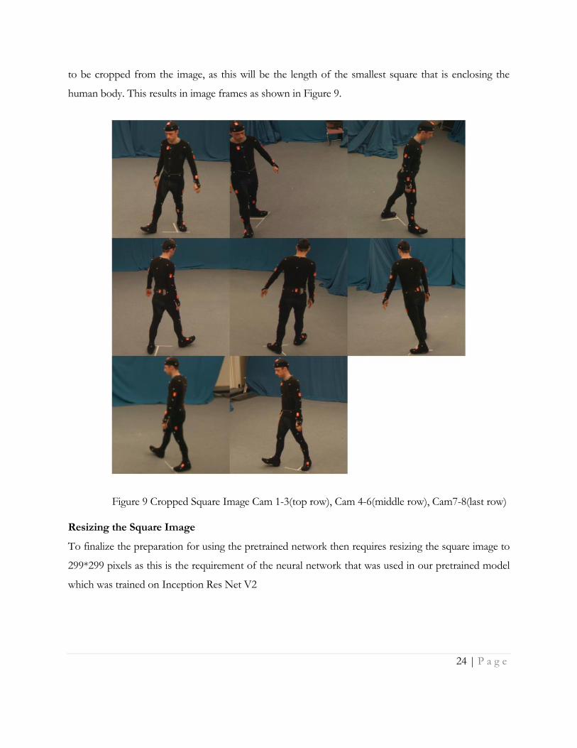
24 | P a g e

to be cropped from the image, as this will be the length of the smallest square that is enclosing the

human body. This results in image frames as shown in Figure 9.

Figure 9 Cropped Square Image Cam 1-3(top row), Cam 4-6(middle row), Cam7-8(last row)

Resizing the Square Image

To finalize the preparation for using the pretrained network then requires resizing the square image to

299*299 pixels as this is the requirement of the neural network that was used in our pretrained model

which was trained on Inception Res Net V2

25 | P a g e

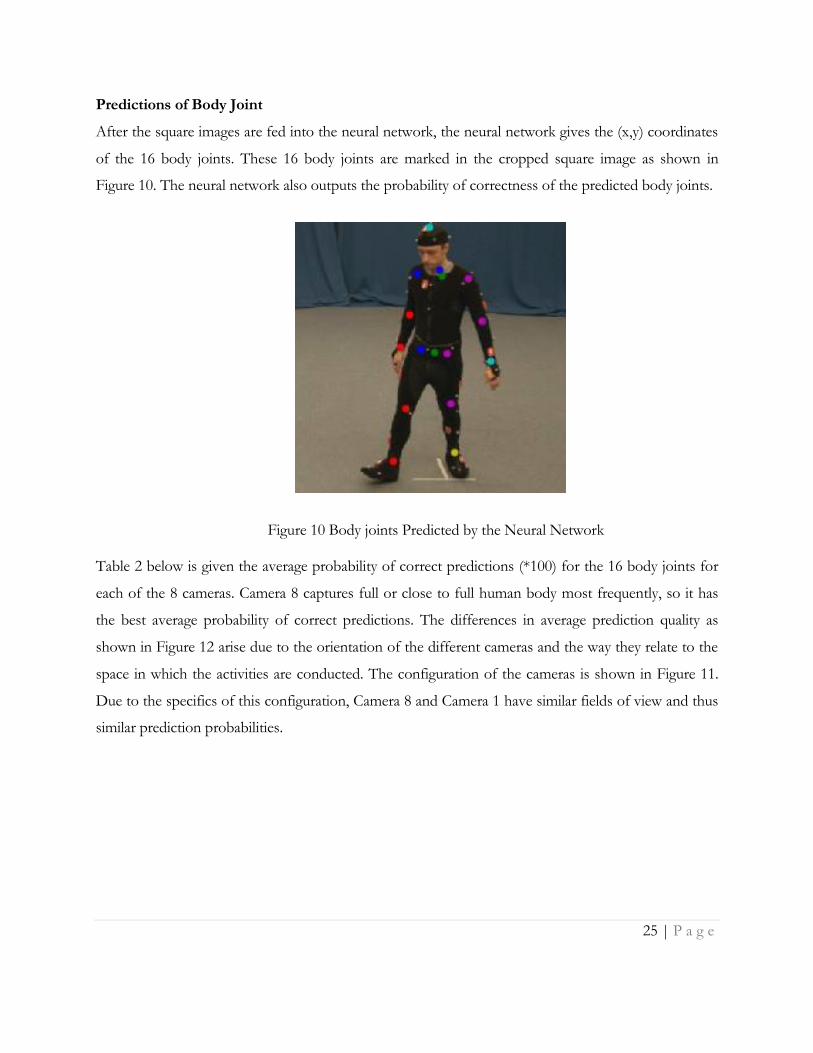
Predictions of Body Joint

After the square images are fed into the neural network, the neural network gives the (x,y) coordinates

of the 16 body joints. These 16 body joints are marked in the cropped square image as shown in

Figure 10. The neural network also outputs the probability of correctness of the predicted body joints.

Figure 10 Body joints Predicted by the Neural Network Table 2 below is given the average probability of correct predictions (*100) for the 16 body joints for

each of the 8 cameras. Camera 8 captures full or close to full human body most frequently, so it has

the best average probability of correct predictions. The differences in average prediction quality as

shown in Figure 12 arise due to the orientation of the different cameras and the way they relate to the

space in which the activities are conducted. The configuration of the cameras is shown in Figure 11.

Due to the specifics of this configuration, Camera 8 and Camera 1 have similar fields of view and thus

similar prediction probabilities.

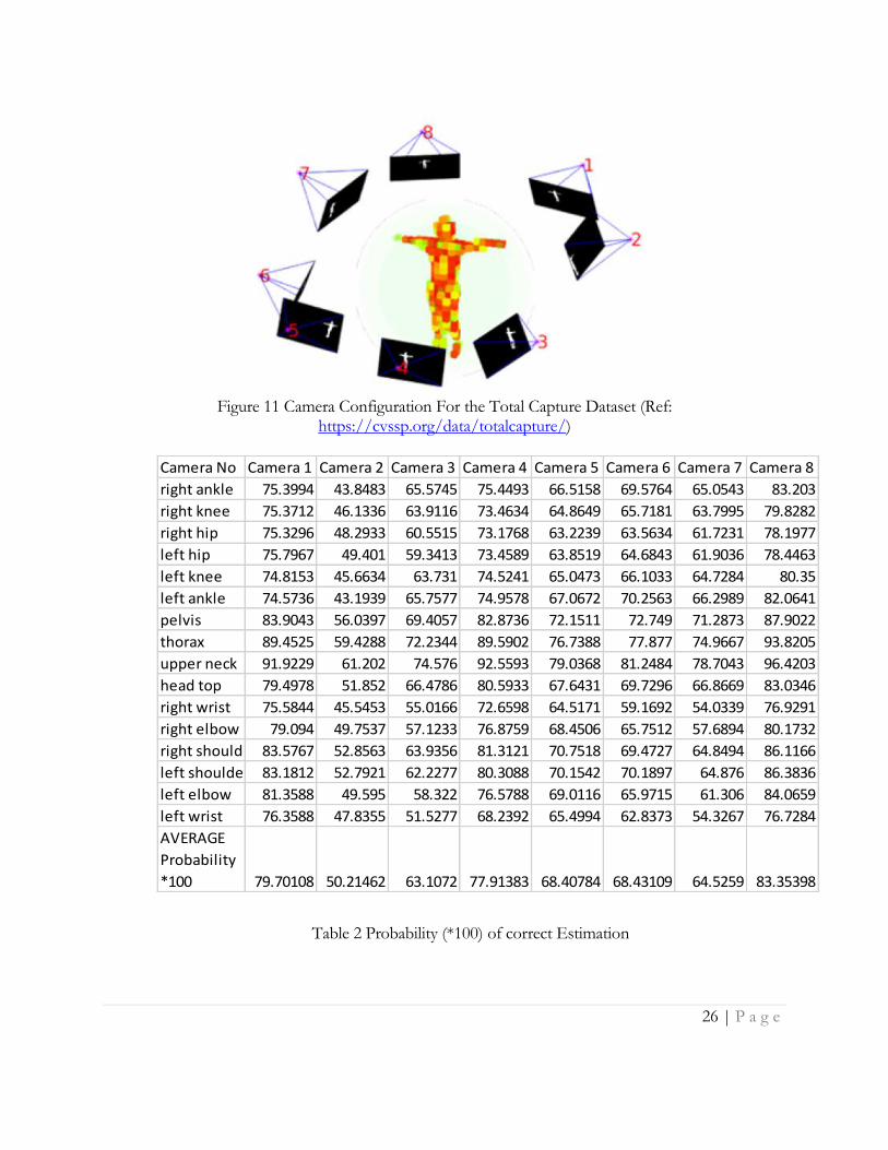
26 | P a g e

Figure 11 Camera Configuration For the Total Capture Dataset (Ref:

https://cvssp.org/data/totalcapture/)

Table 2 Probability (*100) of correct Estimation

Camera No Camera 1 Camera 2 Camera 3 Camera 4 Camera 5 Camera 6 Camera 7 Camera 8

right ankle 75.3994 43.8483 65.5745 75.4493 66.5158 69.5764 65.0543 83.203

right knee 75.3712 46.1336 63.9116 73.4634 64.8649 65.7181 63.7995 79.8282

right hip 75.3296 48.2933 60.5515 73.1768 63.2239 63.5634 61.7231 78.1977

left hip 75.7967 49.401 59.3413 73.4589 63.8519 64.6843 61.9036 78.4463

left knee 74.8153 45.6634 63.731 74.5241 65.0473 66.1033 64.7284 80.35

left ankle 74.5736 43.1939 65.7577 74.9578 67.0672 70.2563 66.2989 82.0641

pelvis 83.9043 56.0397 69.4057 82.8736 72.1511 72.749 71.2873 87.9022

thorax 89.4525 59.4288 72.2344 89.5902 76.7388 77.877 74.9667 93.8205

upper neck 91.9229 61.202 74.576 92.5593 79.0368 81.2484 78.7043 96.4203

head top 79.4978 51.852 66.4786 80.5933 67.6431 69.7296 66.8669 83.0346

right wrist 75.5844 45.5453 55.0166 72.6598 64.5171 59.1692 54.0339 76.9291

right elbow 79.094 49.7537 57.1233 76.8759 68.4506 65.7512 57.6894 80.1732

right shoulder 83.5767 52.8563 63.9356 81.3121 70.7518 69.4727 64.8494 86.1166

left shoulder 83.1812 52.7921 62.2277 80.3088 70.1542 70.1897 64.876 86.3836

left elbow 81.3588 49.595 58.322 76.5788 69.0116 65.9715 61.306 84.0659

left wrist 76.3588 47.8355 51.5277 68.2392 65.4994 62.8373 54.3267 76.7284

AVERAGE

Probability

*100 79.70108 50.21462 63.1072 77.91383 68.40784 68.43109 64.5259 83.35398

27 | P a g e

Figure 12 Average Probability of Correct Prediction for Each of the 8 Cameras Creating a Body Skeleton

The predicted body joints are connected with lines such that a body skeleton is created. The coloring

scheme for joining the body joints is :-

• Right Ankle to Right Knee – Red

• Right Knee to Right Hip – Red

• Right Hip to Pelvis – Blue

• Pelvis to Left Hip – Blue

• Left Hip to Left Knee – Magenta

• Left Knee to Left Ankle – Magenta

• Pelvis to Thorax – Green

• Thorax to Upper Neck – Green

• Upper Neck to Head Top – Blue

• Right Wrist to Right Elbow – Red

• Right Elbow to Right Shoulder – Red

• Right Shoulder to Left Shoulder – Blue

• Left Shoulder to Left Elbow – Magenta

• Left Elbow to Left Wrist - Magenta

0 10 20 30 40 50 60 70 80 90

1

2

3

4

5

6

7

8

Average Estimation Probability Per Camera

28 | P a g e

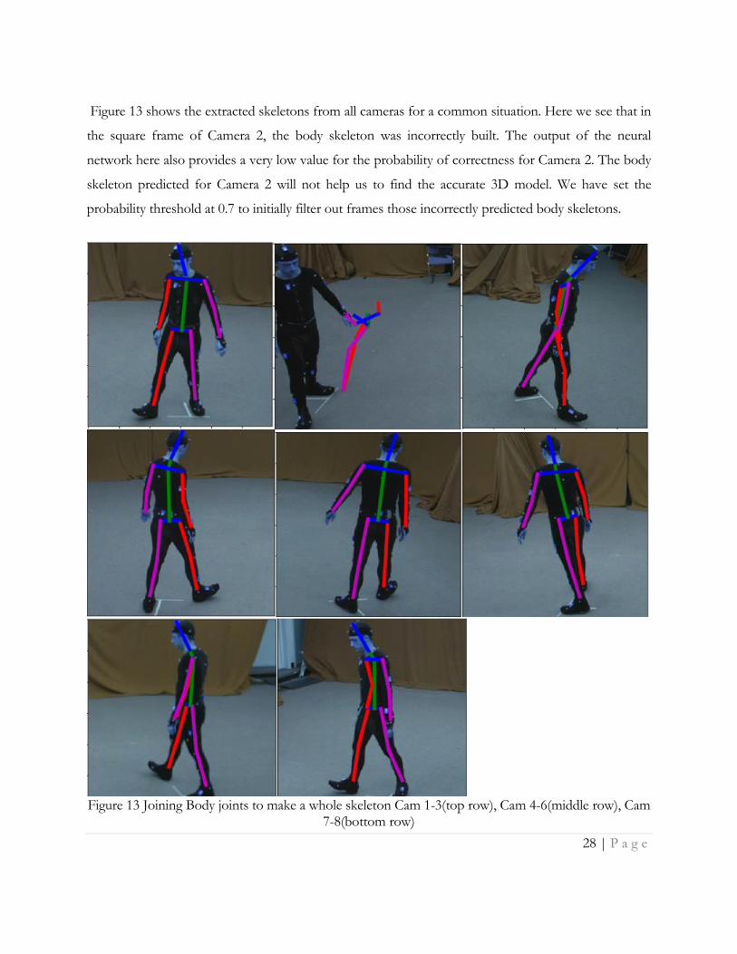
Figure 13 shows the extracted skeletons from all cameras for a common situation. Here we see that in

the square frame of Camera 2, the body skeleton was incorrectly built. The output of the neural

network here also provides a very low value for the probability of correctness for Camera 2. The body

skeleton predicted for Camera 2 will not help us to find the accurate 3D model. We have set the

probability threshold at 0.7 to initially filter out frames those incorrectly predicted body skeletons.

Figure 13 Joining Body joints to make a whole skeleton Cam 1-3(top row), Cam 4-6(middle row), Cam

7-8(bottom row)

29 | P a g e

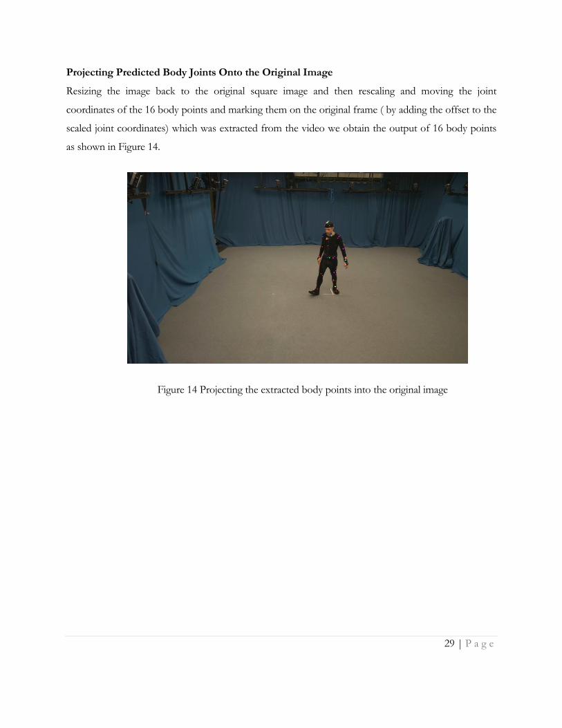
Projecting Predicted Body Joints Onto the Original Image

Resizing the image back to the original square image and then rescaling and moving the joint

coordinates of the 16 body points and marking them on the original frame ( by adding the offset to the

scaled joint coordinates) which was extracted from the video we obtain the output of 16 body points

as shown in Figure 14.

Figure 14 Projecting the extracted body points into the original image

30 | P a g e

C h a p t e r 4

THE 3D SKELETON

To extract a 3D skeleton model from the visual 2D skeleton models extracted in Chapter 3, the

multiple camera views have to be combined into a consistent 3D model. To achieve this, a number of

challenges have to be addressed. The first challenge her is that in general the pose of the cameras is not

known a priori. It is thus necessary to automatically learn the pose parameters in order to obtain

consistent estimates. In addition, as indicated previously, the 2D skeleton extraction can sometimes

yield incorrect skeleton models. The presence of incorrect or inaccurate models, in turn, yields

inconsistent integration results and it is thus important to be able to correctly select the best camera

views at each point in time. As a general rule here, more consistent camera views should yield better

and more robust results while inclusion of incorrect views will lead to highly incorrect results, As a

result it would be desirable to obtain 3D information using the largest number of consistent camera

views while eliminating inconsistent and incorrect views.

To address these challenges we need to first establish a consistent estimate of the poses of the

cameras.

Camera Matrix

In computer vision a camera matrix or (camera) projection matrix is a {3*4} matrix which describes

the mapping of a pinhole camera from 3D points in the world to 2D points in an image.

Let x be a representation of a 3D point in homogeneous coordinates (a 4-dimensional vector), and

let y be a representation of the image of this point in the pinhole camera (a 3-dimensional vector).

Then the following relation holds:

y ~ Cx

where C is the camera matrix and ~ implies that the left and right hand sides are proportional, i.e.

equal up to a non-zero scalar multiplication.

31 | P a g e

Since the camera matrix C is involved in the mapping between elements of two projective spaces, it

too can be regarded as a projective element. This means that it has only 11 degrees of freedom since

any multiplication by a non-zero scalar results in an equivalent camera matrix.

The camera matrix which relates points in the coordinate system (X1', X2', X3') to image coordinates

is

C = (R |T)

where R is the 3D rotation matrix and T is the 3D translation vector. Thus, C is the concatenation of

R and T which makes it a 3*4 dimensional matrix.

The camera matrix describes the optical characteristics and pose of each camera. We plan to get the

3D skeleton from multiple 2D skeleton which were extracted for every camera view. We thus need to

determine the relative pose of each camera with respect to the other cameras. To do this, we need to

determine the camera matrix for each of the cameras from the 2D skeleton data. This can be achieved

by reversing triangulation since all cameras are observing the same 3D skeleton and thus the 3D points

represent the triangulation result of the separate 2D camera views.

Triangulation

In computer vision triangulation refers to the process of determining a point in 3D space given its

projections onto two, or more, images. If a pair of corresponding points in two, or more images, can

be found it must be the case that they are the projection of a common 3D point x. If the camera

matrix for each of the cameras is known, the location of a particular joint in each camera view

corresponds to a beam in space and the 3D location is the intersection (or the point closest to each of

the lines in case of noise that precludes intersection). Note, that as the camera matrix is unique only up

to scaling, the 3D location will also be correct only up to scaling. Figure 15 shows an example of the

triangulation geometry for 4 separate camera views.

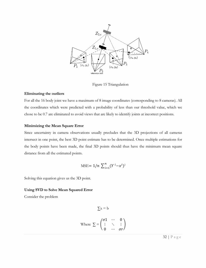
32 | P a g e

Figure 15 Triangulation

Eliminating the outliers

For all the 16 body joint we have a maximum of 8 image coordinates (corresponding to 8 cameras). All

the coordinates which were predicted with a probability of less than our threshold value, which we

chose to be 0.7 are eliminated to avoid views that are likely to identify joints at incorrect positions.

Minimizing the Mean Square Error

Since uncertainty in camera observations usually precludes that the 3D projections of all cameras

intersect in one point, the best 3D point estimate has to be determined. Once multiple estimations for

the body points have been made, the final 3D points should thus have the minimum mean square

distance from all the estimated points.

MSE= 1/𝑛 ∑ (𝑌 𝑖−𝑥𝑖)𝑛

𝑖=12

Solving this equation gives us the 3D point.

Using SVD to Solve Mean Squared Error

Consider the problem

∑x = b

Where ∑ = (𝜎1 ⋯ 0⋮ ⋱ ⋮0 ⋯ 𝜎𝑟

)

33 | P a g e

Note that b is in the range of ∑ if its entries br+1 to bn are all zero. The least squares solution here must

be

x = (b1/σ1,…,br /σr,0,…,0)T = ∑-1 b So for the equation –

U∑VTX = b => ∑VTX = U-1b = UTb Using the above argument, the least square solution for ||VTX|| = ∑-1UTb where||VTX|| =

||X||, concluding that ∑-1UTb must be the least square solution for X.

Using this we can construct the Camera projection matrices as the ones that lead to the least square

error reconstruction in 3D. Given two points we first formulate this in homogeneous coordinates,

constructing a 3*4 matrix (say A). We then find the least square solution for AX =0. In our case we

have computed Singular Value Decomposition[1] of A.

[U,d,V] = SVD(A)

U is a n × k matrix with orthonormal columns, UTU = Ik, where Ik is the k × k identity matrix.

V is an orthonormal k × k matrix, VT = V−1.

S is a k ×k diagonal matrix, with the non-negative singular values, s1, s2, . . . , sk, on the diagonal. By

convention the singular values are given in the sorted order s1 ≥ s2 ≥ . . . ≥ sk ≥ 0.

We take the last column of matrix V, that gives our solution in 4 dimensional space, associated with

homogeneous coordinate of a point in 3D. To convert this point into physical space, we need to take

out the last element of the homogeneous coordinate, i.e. the fourth dimension and we get a point in 3

dimensional space.

34 | P a g e

It can be observed that the camera matrix represents both intrinsic camera parameters (e.g. focal

length, image centering, or distortion) and extrinsic parameters (the location and orientation of the

camera).

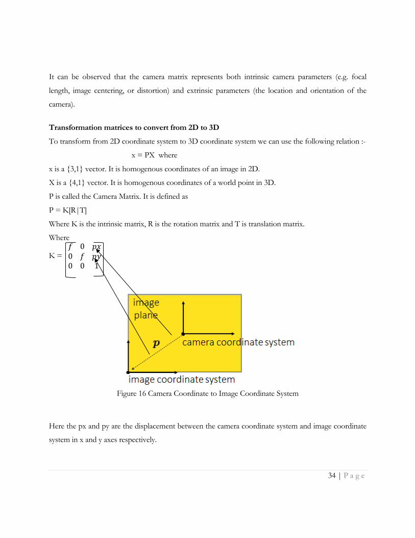
Transformation matrices to convert from 2D to 3D

To transform from 2D coordinate system to 3D coordinate system we can use the following relation :-

x = PX where

x is a {3,1} vector. It is homogenous coordinates of an image in 2D.

X is a {4,1} vector. It is homogenous coordinates of a world point in 3D.

P is called the Camera Matrix. It is defined as

P = K[R|T]

Where K is the intrinsic matrix, R is the rotation matrix and T is translation matrix.

Where

K = 𝑓 0 𝑝𝑥0 𝑓 𝑝𝑦0 0 1

Figure 16 Camera Coordinate to Image Coordinate System

Here the px and py are the displacement between the camera coordinate system and image coordinate

system in x and y axes respectively.

35 | P a g e

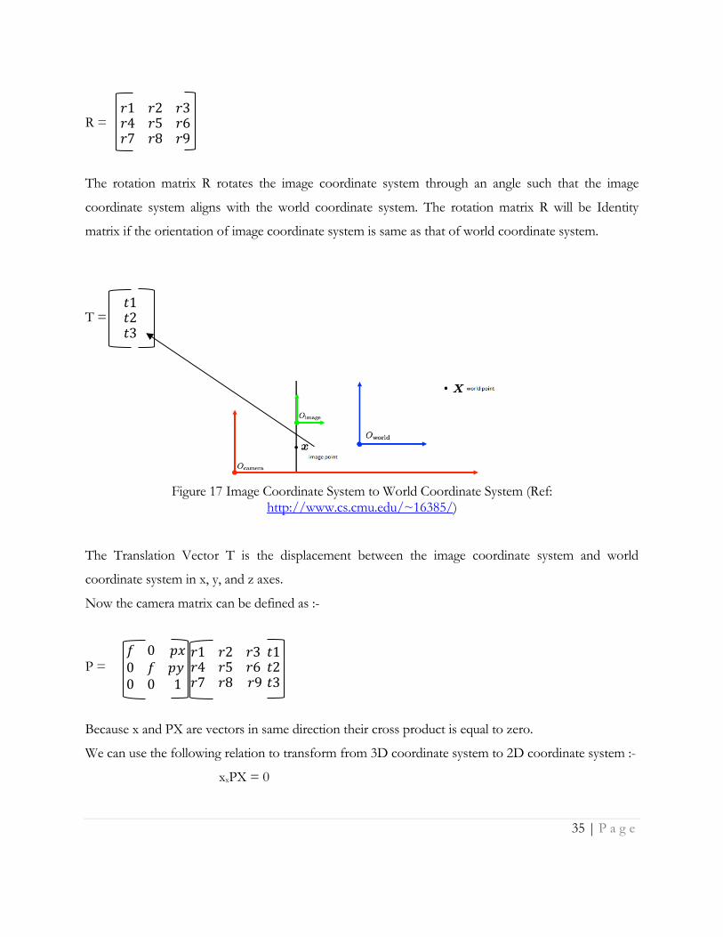
R = 𝑟1 𝑟2 𝑟3𝑟4 𝑟5 𝑟6𝑟7 𝑟8 𝑟9

The rotation matrix R rotates the image coordinate system through an angle such that the image

coordinate system aligns with the world coordinate system. The rotation matrix R will be Identity

matrix if the orientation of image coordinate system is same as that of world coordinate system.

T = 𝑡1𝑡2𝑡3

Figure 17 Image Coordinate System to World Coordinate System (Ref:

http://www.cs.cmu.edu/~16385/) The Translation Vector T is the displacement between the image coordinate system and world

coordinate system in x, y, and z axes.

Now the camera matrix can be defined as :-

P = 𝑓 0 𝑝𝑥0 𝑓 𝑝𝑦 0 0 1

𝑟1 𝑟2 𝑟3 𝑟4 𝑟5 𝑟6 𝑟7 𝑟8 𝑟9

𝑡1𝑡2𝑡3

Because x and PX are vectors in same direction their cross product is equal to zero.

We can use the following relation to transform from 3D coordinate system to 2D coordinate system :-

xxPX = 0

36 | P a g e

For our 2 camera example consider the respective intrinsic parameters K1 and K2 which both are 3*3

matrices. Combining this with the extrinsic pose parameters the camera projection matrices P1 and P2

are defined as follows –

P1 = K1*[Rotation Matrix(3*3) | Translation Vector(3,1)]

P2 = K2*[Rotation Matrix(3*3) | Translation Vector(3,1)]

If we have two points x1 and x2 in 2 Dimensional space, we write them in homogeneous form

converting them to 3*1 vectors.

We convert x1 and x2 into skew form, which converts 3*1 vectors into 3*3 matrices of the form :-

[0 -x(3) x(2); x(3) 0 -x(1); -x(2) x(1) 0]

Giving us a matrix containing the views of both cameras:

A = [ skew1*P1; skew2*P2];

As we have 8 cameras we will have 8 Projection matrices P1, P1 … P8 and 8 skew matrices skew1,

skew2 … skew8.

In that case

A = [ skew1*P1; skew2*P2; skew3*P3; skew4*P4; skew5*P5; skew6*P6; skew7*P7; skew8*P8]

[u,d,v] = SVD(A)

X = v(:,end)/v(end,end)

Here X is a 4*1 vector with the 4th element being equal to 1, representing the homogeneous coordinate

of the estimated point.

37 | P a g e

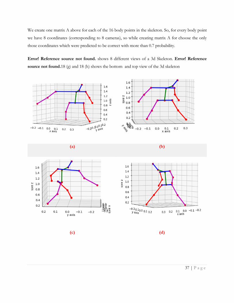
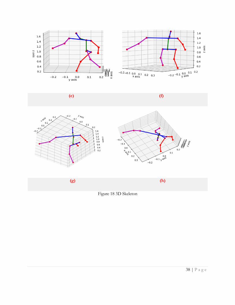
We create one matrix A above for each of the 16 body points in the skeleton. So, for every body point

we have 8 coordinates (corresponding to 8 cameras), so while creating matrix A for choose the only

those coordinates which were predicted to be correct with more than 0.7 probability.

Error! Reference source not found. shows 8 different views of a 3d Skeleton. Error! Reference

source not found.18 (g) and 18 (h) shows the bottom and top view of the 3d skeleton

(a) (b)

(c) (d)

38 | P a g e

(e) (f)

(g) (h)

Figure 18 3D Skeleton

39 | P a g e

C h a p t e r 5

EXTRACTING DETAILS ABOUT BODY GAIT CHARACTERISTICS

The main goal of extracting the skeleton is to be able to model gait characteristics. In the TotalCapture

dataset used here, in addition to the multi-view video data, wearable sensor data from 13 9-axis

accelerometer/gyroscope/magnetometer sensors mounted on different links of the body is available

and permits comparison of accuracies achieved using 2D, 3D, and wearable sensor data. It is

important to note here that since wearable IMUs inherently record dynamics, they shoud be expected

to be more capable of detecting dynamic conditions (such as impacts or movements) while visual 2D

or 3D data should be better at identifying spatial characteristics (such as lengths and configurations).

To investigate this, we designed systems that try to predict a number of these characteristics.

Classification of Leg State While Walking:

The first gait characteristic we are trying to predict is which of the fundamental phases of the gait the

person is in, namely the base types of stance phases in a gait cycle:

1. Single Support (Right Leg in motion)

2. Single Support (Left Leg in motion)

3. Double Support (Standing on both feets)

Figure Error! Reference source not found. shows example of the different stance phases. Learning

to classify these three states of human gaits while walking can be very helpful in analyzing the gait of a

human. If we are able to get the above three states the following gait features can be analyzed :-

1. Step time which is the time between two consecutive heel strikes.

2. Single support the time over which the body is supported by only one leg

3. Double support the time over which the body is supported by both legs

4. Swing time which is the time for the leg to swing through while the body is in single support

on the other leg

40 | P a g e

5. Cadence which is the number of steps taken in a given time, usually steps per minute

6. Stride length which is defined as the distance between successive ground contacts of the same

foot.

7. Gait velocity (Average) the stride length divided by the stride time.

Figure 19 Single Support (Left Leg), Single Support (Right Leg), Double Support

As indicated, we build models for 3 sensor inputs, namely wearable sensor data, 2D image data, and

3D skeleton data to allow comparisons. It is important to note here that since the stance phases have

strong dynamic component differences since in single support usually one leg is moving in the air, we

could expect some advantages from the use of wearable sensors for this. However, the use of 13

wearable sensor packages is somewhat unrealistic for real world use of the techniques and thus vision-

based systems would be preferable.

41 | P a g e

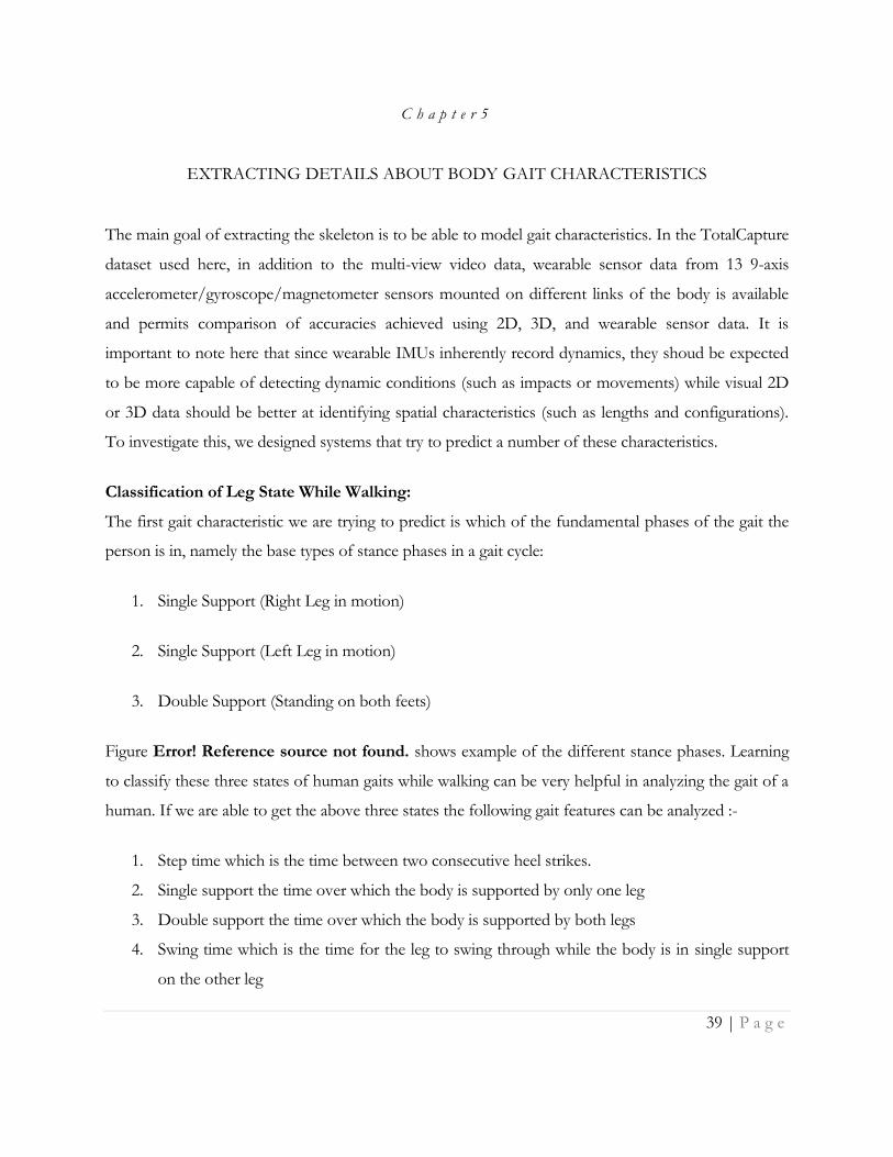
Classifying Walking State from the Sensors data:

A neural network was created with the IMU sensor data of the human body as the input and the three

states of the gait as the output. The neural network used for this task was a 5 layer network with dense

layers and a total of 1580 trainable weights as shown in Table 3.

Table 3: Summary Neural Network for sensors data

After training the model we obtain a validation accuracy of 93% and a training accuracy of 97.5%. The

model was trained for 30 epochs. Figure 180Error! Reference source not found. shows the training

loss and validation for each of the training epochs, illustrating the learning progress.

Figure 191 shows training accuracy and validation accuracy vs no. of epochs.

42 | P a g e

Figure 180 Model Loss from Sensors Data

Figure 191 Model Accuracy from Sensors Data

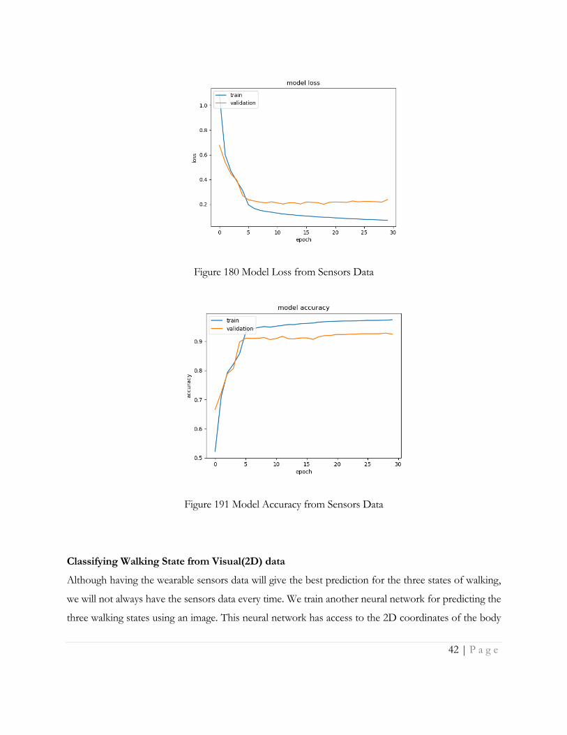
Classifying Walking State from Visual(2D) data

Although having the wearable sensors data will give the best prediction for the three states of walking,

we will not always have the sensors data every time. We train another neural network for predicting the

three walking states using an image. This neural network has access to the 2D coordinates of the body

43 | P a g e

joints extracted using the methods from Chapter 3. This neural network has two-dimensional

coordinates of the body joints as input data which is 32 points(16*2; 16 body joints estimated and 2

points per body joint ) of the human body and the three states as the output. Again a 5 layer network

is used but the size of the layers was adapted to better work with this data. Table 4 summarizes the

neural network configuration used here.

Table 4: Summary Neural Network for 2D data

After training the model we obtain a validation accuracy of 80% and a training accuracy of 82%. The

model was trained for 30 epochs. Table 4 shows training loss , validation loss vs no. of epochs.

44 | P a g e

Figure 22 Model Loss from 2D Data Figure 203 shows training accuracy and validation accuracy vs no. of epochs.

Figure 203 Model Accuracy from 2D Data

45 | P a g e

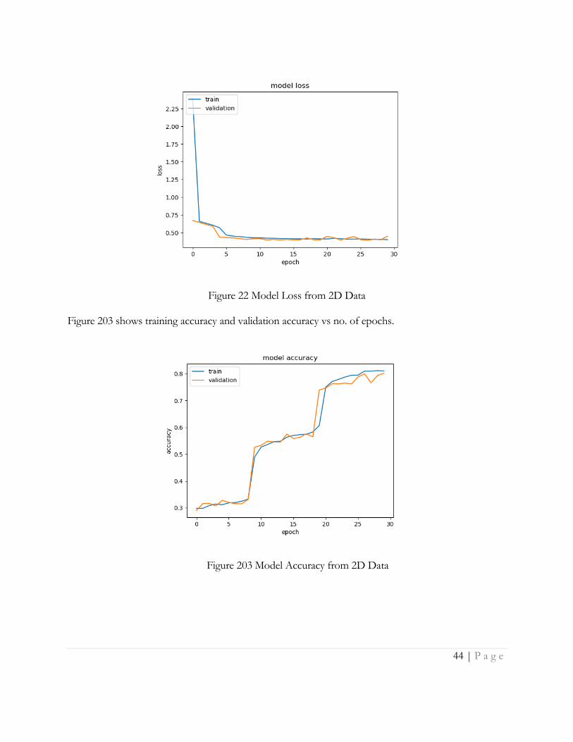
Classifying Walking State from Visual(3D) Data

Now we create a neural network for predicting the three walking states using the 3D human body

model extracted using the techniques described in Chapter 4. This neural network has three-

dimensional coordinates of the body joints as input data which is 48 points(16*3; 16 body joints

estimated and 3 points per body joint ) of the human body and the three states as the output. Figure

214 shows extracted 3D skeleton examples for the 3 stance types, corresponding to the images shown

in Error! Reference source not found.. To address this, again a 5 layer dense network was created.

Table 5 summarizes the neural network configuration which was used for training.

Table 5: Summary Neural Network for 3D data

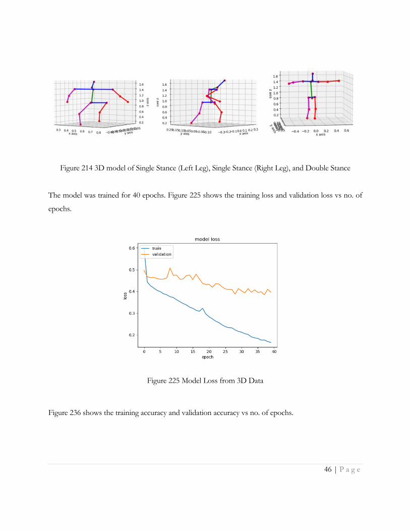
After training the model we obtain a validation accuracy of 88% and training accuracy of 95%. We

have observed that the validation accuracy of the 3D model for classifying the three states of walking

is significantly better than the validation accuracy from the image and only slightly lower than for

wearable sensor data even though it does not contain dynamic information. This illustrates the benefit

of integrating multi-view data for gait analysis.

46 | P a g e

Figure 214 3D model of Single Stance (Left Leg), Single Stance (Right Leg), and Double Stance

The model was trained for 40 epochs. Figure 225 shows the training loss and validation loss vs no. of

epochs.

Figure 225 Model Loss from 3D Data

Figure 236 shows the training accuracy and validation accuracy vs no. of epochs.

47 | P a g e

Figure 236 Model Accuracy from 3D Data

Based on the trained classifiers we can now extract a number of standard gate features such as swing

time, stride length, cadence, or gait velocity. For this we developed algorithms and an application.

Calculating the Swing Time

As our neural network is able to identify the frames of the video when the human body is in Single

support, we can find the difference of the number of frames between when the Single support of the

leg starts and when it ends. As we know the frame rate for the video, we can calculate the swing time.

Calculating the Time to Complete the Stride

The time to complete the stride is the sum of times of two consecutive swing cycles plus two

consecutive double stance cycles.

Calculating the stride length

After getting the 3D models of the sequence calculating the stride length can be found by finding the

L2 distance between the 3D coordinates of “Pelvis”, by getting the difference between the two time

stamps which correspond to the start and end time of a complete the stride.

Stride Length = np.sqrt(np.square(XCoordinateOfPelvis2 – XcoordinateOfPelvis1) +

48 | P a g e

np.square(YcoordinateOfPelvis2 - YcoordinateOfPelvis1) +

np.square(ZcoordinateOfPelvis2 - ZcoordinateOfPelvis1))

Calculating the Cadence

As we have already calculated the time to complete the stride and stride length, we can easily compute

cadence as the inverse of the stride time:

Cadence = 1 minute/ time to complete the stride

Gait Velocity (Average)

Similarly, gait velocity can easily be calculated based on the number of strides, the stride length and the

duration (or alternatively based on cadence and stride length):

Gait velocity = no. of strides * stride length/ total time of walking

Gait velocity = stride length/cadence

Web Application

To visualize the gait parameters extracted, we have developed a Web Application which displays gait

characteristics along with video being played. Figure 27 shows a screenshot of the application

analyzing the video.

49 | P a g e

Figure 27 Application Displaying Video and Gait Analysis

In this figure, the actor is seen moving his left leg as predicted by the neural network for the 3D data.

Other gait characteristics like Swing Time, Distance covered in current swing, Cadence, Stride Time is

also displayed.

50 | P a g e

C h a p t e r 6

CONCLUSION

The estimation of a 3D body skeleton from multiple viewpoint video (MVV) is a potentially powerful

but less explored area. In this thesis we were successfully able to estimate 3D body pose and used it for

gait analysis.

To obtain the 3D skeleton we first estimated a 2D body skeleton in each of the camera views using

Transfer learning. We were able to successfully use pretrained models learned from datasets like

Human3.6M, Max Planck Institute’s MPII Dataset and Leeds Sports Pose Dataset and apply them to

the multi-view video in the Total Capture Dataset. This 2D skeleton data were then fused together to

construct the 3D skeleton of the human body using triangulation. In this process, outliers (i.e.

incorrect skeletons were automatically removed and camera parameters were generated to provide the

most consistent reconstruction.

Using the video, extracted 3D skeleton, and wearable sensor data, we then developed three neural

networks for classifying the distinct gait phases. The outputs of these neural networks for gait

characteristics were evaluated against ground truth.

This evaluation demonstrates that the neural networks were able to classify among the three states of

walking. We have found that Neural Network using sensors data has the best accuracy, likely due to its

direct access to dynamics information, followed closely by 3D body skeletons, and more distantly 2D

body skeletons. This illustrated the benefit of multi-view skeleton extraction for gait analysis.

Using this classification, other gait characteristics like Cadence, Gait Velocity, Step time, Stride time,

Swing time were also extracted. And an application was also built to demonstrate the values of these

gait characteristics corresponding to the input video sequence.

51 | P a g e

BIBLIOGRAPHY

[1] The Singular Value Decomposition Prof. Walter Gander, Zurich. Pulished in 2008

[2] Peng Huang · Adrian Hilton · Jonathan Starck. Shape Similarity for 3D Video Sequences of

People. Springer Science+Business Media, LLC 2010.

[3] Xiaowei Zhou, Menglong Zhu, Spyridon Leonardos, Konstantinos G. Derpanis, Kostas

Daniilidis. Sparseness Meets Deepness: 3D Human Pose Estimation from Monocular Video.

2016.

[4] Marta Sanzari, Valsamis Ntouskos, and Fiora Pirri. Bayesian Image Based 3D Pose

Estimation. Springer International Publishing AG 2016.

[5] T. von Marcard, B. Rosenhahn, M. J. Black, G. Pons-Moll. Sparse Inertial Poser: Automatic

3D Human Pose Estimation from Sparse IMUs. The Eurographics Association and John

Wiley & Sons Ltd. 2017

[6] Matthew Loper, Naureen Mahmood, Javier Romero, Gerard Pons-Moll, Michael J. Black.

SMPL: A Skinned Multi-Person Linear Model. ACM Transactions on Graphics October

2015.

[7] Hao Jiang. Human Pose Estimation Using Consistent Max-Covering. IEEE International

Conference on Computer Vision 2009(ICCV 2009).

[8] Catalin Ionescu, Dragos Papava, Vlad Olaru, and Cristian Sminchisescu. Human3.6M: Large

Scale Datasets and Predictive Methods for 3D Human Sensing in Natural Environments.

IEEE transactions on pattern analysis and machine ingelligence, VOL. 36, NO. 7, JULY

2014.

[9] Andrew Gilbert, Matthew Trumble, Adrian Hilton, John Collomosse, Charles Malleson.

Total Capture: 3D Human Pose Estimation Fusing Video and Inertial Sensors. University of

Surrey Guildford, UK.

[10] Hansong Zeng and Yi Zhao. Sensing Movement: Microsensors for Body Motion

Measurement. Sensors, 2011.

[11] Weijun Tao, Tao Liu, Rencheng Zheng, and Hutian Feng. Gait Analysis Using Wearable

Sensors. Sensors 2012.

52 | P a g e

[12] X. Lan and D. Huttenlocher. Beyond trees: common-factor model for 2d human

pose recovery. In Proc. Intl. Conf. on Computer Vision, volume 1, pages 470–477, 2005.

[13] Timo von Marcard, Gerard Pons-Moll, and Bodo Rosenhahn. Human pose estimation from

video and imus. IEEE transactions on pattern analysis and machine intelligence, 38(8):1533–

1547, 2016.

[14] Corazza, S., E. Alexander, A. Chaudhari, C. Cobelli, and T. Andriacchi. Surface from

silhouette reconstruction for markerless motion capture. In Proceedings of the 7th

Symposium Comp. Methods in Biomech., Madrid Spain, 2004.]

[15] Thomas Helten, Meinard Muller, Hans-Peter Seidel, and Christian Theobalt. Real-time body

tracking with one depth camera and inertial sensors. In Proceedings of the IEEE

International Conference on Computer Vision, pages 1105–1112, 2013.

[16] Bregler, C., and J. Malik. Tracking people with twists and exponential maps. Proc. IEEE

CVPR 8–15, 1998.

53 | P a g e

DATA SET REFERENCES

1. Marian margeta – gait recognition - MPII+LSP.ckpt

2. Marian margeta - gait recognition - Human3.6m.ckpt

3. Total Capture Dataset - https://cvssp.org/data/totalcapture/

4. Inception Resnet v2 https://ai.googleblog.com/2016/08/improving-inception-and-

image.html

5. Max Planck Institute Dataset - https://www.mpi-inf.mpg.de/departments/computer-vision-

and-machine-learning/software-and-datasets/

6. Leeds Sports Dataset - https://sam.johnson.io/research/lspet.html