3D SIMULATION OF MAGNETOTELLURIC DATA

USING FINITE DIFFERENCE EIGENMODE METHOD

Ph.D. THESIS

by

KRISHNA KUMAR

DEPARTMENT OF EARTH SCIENCES INDIAN INSTITUTE OF TECHNOLOGY ROORKEE

ROORKEE - 247 667 (INDIA) AUGUST, 2009

3D SIMULATION OF MAGNETOTELLURIC DATA USING FINITE DIFFERENCE EIGENMODE METHOD

A THESIS

Submitted in partial fulfilment of the

requirements for the award of the degree

of

DOCTOR OF PHILOSOPHY

in

EARTH SCIENCES

by

KRISHNA KUMAR

DEPARMENT OF EARTH SCIENCES INDIAN INSTITUTE OF TECHNOLOGY ROORKEE

ROORKEE-247 667 (INDIA) AUGUST, 2009

©INDIAN INSTITUTE OF TECHNOLOGY ROORKEE, ROORKEE, 2009 ALL RIGHTS RESERVED

INDIAN INSTITUTE OF TECHNOLOGY ROORKEE ROORKEE

CANDIDATE’S DECLARATION

I hereby certify that the work which is being presented in the thesis entitled 3D

SIMULATION OF MAGNETOTELLURIC DATA USING FINITE DIFFERENCE

EIGENMODE METHOD in partial fulfilment of the requirements for the award of the

Degree of Doctor of Philosophy and submitted in the Department of Earth Sciences of the

Indian Institute of Technology Roorkee, Roorkee is an authentic record of my own work

carried out during a period from July, 2004 to August, 2009 under the supervision of Dr. Sri

Niwas, Professor and Dr. Pravin K. Gupta, Professor, Department of Earth Sciences, Indian

Institute of Technology Roorkee, Roorkee.

The matter presented in the thesis has not been submitted by me for the award of any

other degree of this or any other Institute.

(KRISHNA KUMAR)

This is to certify that the above statement made by the candidate is correct to the best

of our knowledge.

(Pravin K. Gupta) (Sri Niwas) Supervisor Supervisor

Date:

The Ph.D. Viva-Voice Examination of Mr. KRISHNA KUMAR, Research Scholar,

has been held on ______________

Signature of Supervisors Signature of External Examiner

iii

ABSTRACT

Magnetotelluric method is used to delineate the subsurface conductivity structure of

earth using natural electromagnetic waves in the frequency range 10-5 Hz – 105 Hz as

source field. These natural fields are generated mainly by thunderstorm activity (>1 Hz)

and the interaction of solar wind with the earth’s magnetosphere (<1 Hz) (Kaufman and

Keller, 1981). The horizontal electric and magnetic field components are measured at the

earth’s surface and analyzed to infer electrical resistivity distribution in the earth’s interior.

The two orthogonal horizontal electric field components are linearly related to the two

horizontal magnetic field components through appropriate transfer function (Tikhonov,

1950 and Cagniard, 1953). The depth of penetration of electromagnetic (EM) wave

depends upon its frequency and conductivity distribution of medium.

The EM fields are studied using Maxwell’s equations, coupled in electric (E) and

magnetic field (B) vectors. These equations are transformed into vector Helmholtz equation

for decoupled E-field or B-field. The vector Helmholtz equation is used to solve for the

response of a given earth model. Typical model parameters are geometry of the target and

spatial distribution of conductivity. The estimation of model parameters from the physical

fields, measured on earth surface, is termed as an inverse problem, while the mapping of

model parameters to measured fields is known as a forward problem. For a good inversion

algorithm, an efficient forward modeling code is needed. This work deals with the

development of an efficient 3D forward modeling algorithm.

The popular numerical modeling schemes can be broadly classified into Integral

Equation Methods (IEM) and Differential Equation Methods (DEM) (Finite Difference

Method (FDM), Finite Element Method (FEM)). While IEM can be efficiently used only

iv

for computing the responses of confined targets buried in a layered earth, the DEMs are

capable of modeling arbitrary complex distributions of conductivity. The coefficient matrix

in case of IEM is full but small in size, while in case of DEM it is large but grossly sparse.

In DEMs use of staggered grid is popular, particularly in 3D case, because its use

analytically incorporates the divergence equation of magnetic field. FDM with staggered

grid is used in the present study.

Instead of using FDM to solve the complete Boundary Value Problem (BVP) with

sources, we have first studied fundamental nature of the eigenvalue problem obtained in

case of source free BVP. Eigenvalues and eigenvectors, collectively known as eigenmodes,

exhibit the basic characteristics of the response to a given physical property distribution in

the model. After estimating the eigenmodes for a given geometry and physical property

distribution, the EM response for a given source frequency can be obtained through

superposition of the eigenvectors. In geophysical applications, similar approach was

implemented by Druskin et al. (1994, 1999) and Stuntebeck (2003).

In the eigenmode method, the responses for additional frequencies can be obtained

in negligible time. In contrast, in case of traditional use of FDM to generate multifrequency

responses, one has to re-run the code for each frequency. During evaluation of

superposition coefficients, the eigenvalues appear in the denominator, implying that the

smaller eigenvalues contribute more significantly to the field. Therefore, one need compute

only a subset of the smallest eigenvalues and corresponding eigenvectors for a given

degree of accuracy of field values. For evaluation of this subset, the iterative methods serve

better than the direct methods, particularly in case of 3D problems where the matrix size is

extremely large.

v

The most widely used methods for evaluating a subset of eigenmodes are Krylov

subspace projection methods. In these methods, only product of the matrix with a vector is

needed and, therefore, only non-zero elements of the sparse coefficient matrix need be

stored. Lanczos and Arnoldi methods are two popular Krylov subspace methods. Former is

used for symmetric matrices while the latter is used for non-symmetric matrices.

Before launching the development of 3D code, we gained experience of eigenmode

method by developing 1D and 2D forward modeling codes. The FDM coefficient matrix is

symmetric. In case of 3D, the symmetric coefficient matrix is of large size, which is

reduced in size by using the current divergence equation, to eliminate the z-component of

electric field from expressions. This step transforms the symmetric coefficient matrix to a

nonsymmetric one, albeit of much smaller size. So, Lanczos method is used to obtain the

eigenmodes in 1D and 2D case while Arnoldi method is used in case of 3D. The

eigenmode evaluation subprogram of our algorithm is adapted from the routines of

ARPACK (1997) software which is based on Implicit Restarted Lanczos/Arnoldi Method

(IRLM/IRAM) given by Sorensen et al. (1992). ARPACK works in different modes such

as ‘regular’, ‘shift and invert’ etc. The regular mode is efficient in obtaining largest

magnitude eigenvalues while invert mode is efficient in obtaining smallest magnitude ones.

Since we are interested in the smallest eigenvalues, shift and invert mode is used. Further,

to circumvent the problem of loss of Lanczos vector orthogonality in case of degenerate

eigenvalues, their complete reorthogonalization has been employed.

The development of 3D algorithm was carried out on a PC. As a result, we had to

introduce several I/O detours and had to work under severe limitations imposed on the size

vi

of the grid. Therefore, we designed several appropriate experiments using the coarse grid to

validate the 3D algorithm.

The organization of seven chapters in the thesis is presented next.

In chapter one, the literature review is presented.

In chapter two, the theory for 3D Magnetotellurics using electric field vector

Helmholtz equation, obtained from Maxwell’s equations, is discussed. Different types of

boundary conditions such as domain and interface boundary conditions are described. The

eigenmode problem is formulated and the eigenmodes are used to obtain the EM response

for multi-frequency case. The derivations of response functions, i.e. apparent resistivity and

phase corresponding to both 2D-TE and 2D-TM modes are discussed.

In chapter three implementation of FDM on staggered grid is described. The

domain is discretized into a grid comprising cuboids. We have followed the convention that

electric field components are defined on midpoints of edges while magnetic field

components are defined at the centers of surfaces. The derivation of matrix equation from

the governing partial differential equation and boundary conditions is presented next. The

coefficient matrix obtained is symmetric and about one third of its eigenvalues are zero.

These spurious zero eigenvalues do not contribute to field synthesis. This knowledge is

made use of in reducing the coefficient matrix size to the number of non-zero eigenvalues

by eliminating the vertical component of electric field and working only with the horizontal

components. This step transformed the symmetric coefficient matrix to a non-symmetric

one. A brief review of ARPACK subprograms adapted to determine the eigenmodes is

presented.

vii

In chapter four, the details of various stages of development of algorithm,

MT_3D_EA, are discussed. Starting with symmetric matrix eigenmode evaluation using

Singular Value Decomposition (SVD), the Lanczos and Arnoldi methods in ‘regular’ and

in ‘shift and invert’ modes are presented. In invert mode a matrix equation need be solved

so efficient matrix solvers based on Conjugate Gradient Method and various

preconditioners used are described next. Finally, the algorithm is presented along with

flow charts of important subprograms.

In chapter five, the synthetic experiments designed to test and validate the

algorithms MT_2D_EA and MT_3D_EA are discussed. First we performed different tests

such as grid convergence and no contrast case to check the consistency and accuracy. Then,

we compared the results of 2D version of our algorithm with published results. We studied

two 2D models (simple and complex) taken from COMMEMI (Zhdanov et al., 1997) and

obtained good match with the average values given in the paper. The RMS errors for

simple and complex models are 0.01 and 0.06 respectively. Next we studied the impact on

the field values of using different percentages of eigenmodes. We observed that for

obtaining accurate field values, 5% eigenmodes were sufficient for the conductive block

model whereas for the resistive block 20% eigenmodes were needed for same accuracy. In

the multi-frequency experiment, we studied Weaver (1976) model. We used two grids for

time periods 1s and 10s and generated the responses (true) for these grids. Next we

generated the response at 1s using 10s eigenmodes and vice versa and found excellent fit

with the corresponding true responses. In case of 3D, additional experiment conducted was

to verify that 3D apparent resistivity values converge to corresponding 2D values as the

strike length in one direction is extended. We compared our 3D response with the

viii

published apparent resistivity values of the model described as 3D-2 in COMMEMI report

and found a good fit.

In chapter six, we have used MT_3D_EA algorithm to generate 3D models whose

responses are commensurate with the MT field data acquired by Israil et al. (2008) in

Garhwal Himalaya. Tyagi (2007) and Israil et al. (2008) analyzed this data using WingLink

software, and proposed the first 2D geoelectric model. We used this model as base model

for our study. Using MT_2D_EA algorithm, we generated responses of this model at two

time periods and found excellent match with the corresponding WINGLINK responses.

Due to limited computer resources, we could not run the complex model using MT_3D_EA

algorithm. So, for 3D study we designed a simplified 3D model retaining the dominant

feature of conducting block. We generated the 3D responses for 4 strike length values (20

km, 50 km, 70 km and 100 km) of the conducting body. At 100 km strike length the 3D

response of the model matches well with the 2D response. Finally, we experimented with

the strike-length and the depth of burial of the block and generated equivalent 3D models

that would explain the conducting anomaly in the observed data. The 3D geometry of the

conductive block, buried under the Roorkee-Gangotri profile near MCT, can be taken as 70

km strike, 20-26 km width and 4 km depth and its resistivity is estimated as 8 Ω-m.

However, the detailed 3D study suggests that the conductive block can be approximated as

a 2D one.

In chapter seven, we have discussed the strategies for further improvement of our

algorithm.

ix

LIST OF PUBLICATIONS a) Conference/ Symposia

1. Krishna Kumar, Pravin K. Gupta and Sri Niwas, 2007. 3D Finite Difference

Scheme for magnetotelluric data using the Implicitly Restarted Lanczos Algorithm. National seminar on “Mapping and modeling of deep crustal features using geoelectromagnetic and other geophysical methods”, Department of Applied Geophysics, ISM University, Dhanbad, India.

2. Krishna Kumar, Pravin K. Gupta and Sri Niwas, 2008. Efficient 2D

modeling using Implicitly Restarted Lanczos Method. 7th International conference and exposition on petroleum geophysics “Hyderabad 2008”, Bi-annual conference of Society of Petroleum Geophysicists (SPG), an affiliate society of SEG, January, 14-16, HICC Hyderabad, India.

3. Krishna Kumar, Pravin K. Gupta and Sri Niwas, 2008. Efficient

geomagnetic modeling using Implicitly Restarted Lanczos Method. International conference on tectonics of the Indian subcontinent, March, 3-6, IIT Bombay, Mumbai, India.

4. Krishna Kumar, Pravin K. Gupta and Sri Niwas, 2008. 3D Finite Difference

Scheme for MT data using eigenmodes. 1st Indo-German Workshop on electromagnetic induction studies for complex geological problems, March, 14-18, Lonavala, Mumbai, India.

xi

ACKNOWLEDGEMENTS

Having an opportunity to acknowledge the help I have had, in completing the

research work towards the doctoral degree, is really the thing I have been waiting for. And

here the names first come to my mind are that of my learned supervisors Prof. Pravin K.

Gupta and Prof. Sri Niwas, Department of Earth Sciences, Indian Institute of Technology

Roorkee, who have guided me in real sense. I wish to express my deep sense of gratitude

and appreciation to them for their stimulating supervision with invaluable suggestions,

keen interest, constructive criticisms and constant encouragement during the course of the

present study. I learned a lot from them not only in the academic area but in other spheres

of life also. I wholeheartedly acknowledge their full cooperation that I received from the

very beginning of this work up to the completion in the form of this thesis.

During this research, the department has had two heads; Prof. R. P. Gupta and

Prof. V. N. Singh and most fortunately they encouraged me by extending every sort of help

as and when sought for.

The author is especially thankful to Prof. M. Israil, Department of Earth Sciences

for their invaluable help and advice from time to time as when needed. The author is also

thankful to Dr. Navneet Gupta and Mr. Tarun, Computer Centre, IIT Roorkee, for

providing the computation facility.

The author would like to make a special note of thank to all faculty members of the

Department of Earth Sciences for their co-operation. Thanks are also to Prof. Deepak

Kashyap, Department of Civil Engineering for their constant encouragement during my

research work. The author also acknowledge his deep sense of gratitude to Late Prof. P.

Weidelt, Institute of Geophysics and Meterology,TU Braunschweig, Germany, Prof. B.

xii

Tezkan, Institute for Geophysics, Gottingen, Germany, Dr. K. M. Strack and Dr. Wei Qian,

KMS Technologies, Huston , USA whose critical and timely suggestions proved to be

helpful.

The author is highly obliged and wishes to express my sincere thanks to the

technical staff of the Department of Earth Sciences, especially to Mr. Nayar, Mr. Rakesh,

Mr. V. K. Saini, Mr. S. K. Sharma, who have helped him in all possible ways during the

official work.

The financial support provided by Ministry of Human Resources and Development

(MHRD), New Delhi and KMS Technologies, Huston, USA to complete the present work

is highly acknowledged.

When hurdles appeared insurmountable and target unachievable, the

encouragement and camaraderie of friends helped keep things in perspective. Author

wishes special thank to his lovely friends, who helped lighten the burden, especially to

Sandy, Vikram, Parmanand, Arun, Navin, Birju, Mukesh, Azad, Suneet, Dr. D. K. Tyagi,

Dr. Anurag Gaur, Vishal, Yogesh, Kuldeep rana, Vijay (Mota bhai), Dr. Pundeer, Dr.

Neer, Dr. Tiwari, Deepak (Tinnu), Nagesh, Nigmanand ojha, Dr. Parminder, Dr.

Ajay Kumar, Dr. Amrish, Dr. Sandeep, Dr. Nitin, Dr. Sapan, Dr. Aman Pal, Dr.

Nirpendra,DR. R. K. Rai., Dr. R. K. Chauhan, P. K. R. Gautam, Ritesh, Pankaj,

Nitil, Anuj, Rahul, R. B. S. yadav, Rajiv Rana, Ankit, Raghu, Yashpal, Sonu Dhiman,

Dikku, Anil Boyal, Rajiv, Najim, Varun.

I also want to thank to Dr. Manoj, Dr. Gaurav, Mrs. Rama, Dr. Niti, Aditya, and

Nandini. The help provided by Mr. Ramesh Chand during write up of the thesis is

especially acknowledged.

xiii

The ever enthusiastic help of my family members, uncles, Shri Parmal Singh, Shri

Giriraj Singh, aunties, Smt. Savitri Devi, Smt Rajbala Devi , brothers Shiv Hari, Pravin,

Vipin, Pawan, and sister Pavitra , bhabhi, Santosh and Nirmesh who were distant to me

but were always by his side whenever the need so arrived and accompany for me to work

peacefully during the study period. I am in dearth of proper words to express my

abounding feelings and affection for my lovely Jiju Devendra Yadav and sister Reena. The

author is also thankful to my lovely and cute nephews and nieces Aman, Abhishek,

Mayank, Taksha, Ayush and Ayushi.

I express my heartily gratitude to Smt. Shashi Pandey, Smt. Mamta Gupta and Smt.

Saeeda as time spent occasionally during tea ,dinner was very pleasant.

Finally, I express my heartfelt gratitude to my highly respectable and adorable

father, Shri Dharam Veer Singh and mother, Smt. Kamlesh Devi for their unconditional

love, encouragement and blessings. Words can never express my feelings for them. They

have been a guiding force all his life and he tried to measure up to their expectations. I also

express my abounding feelings of gratitude to all those who helped me in this course but

have not been listed here.

At last thanks to the almighty god who has given the author spiritual support and

courage to carry out this work.

I.I.T. Roorkee (Krishna Kumar)

August, 2009

xv

CONTENTS

Page No. CANDIDATE’S DECLARATION i

ABSTRACT iii

LIST OF PUBLICATIONS ix

ACKNOWLEDGEMENTS xi

CONTENTS xv

LIST OF FIGURES xix

LIST OF TABLES xxiii

CHAPTER 1 INTRODUCTION 1-19

1.1 Applications of Electromagnetic Methods 2

1.1.1 Crustal studies 2

1.1.2 Geothermal studies 3

1.1.3 Marine EM studies 4

1.2 Interpretation of EM Data 4

1.3 Numerical Modeling 9

1.4 Krylov Methods 13

1.4.1 Lanczos/Arnoldi methods 14

1.5 About the Present Work 17

CHAPTER 2 THEORY OF MAGNETOTELLURIC METHOD 21-34

2.1 Introduction 21

2.2 Electromagnetic Theory 22

2.3 About Origin of MT Source 24

2.4 Boundary Value Problem 25

2.4.1 Interface boundary conditions 26

2.4.2 Domain boundary conditions 27

2.5 Eigenmode Formulation of EM Problem 28

2.6 MT Response Function 31

2.6.1 MT apparent resistivity and phase 32

xvi

CHAPTER 3 FINITE DIFFERENCE IMPLEMENTATION 35-51

3.1 Introduction 35

3.2 Finite Difference Implementation 36

3.2.1 Implementation of staggered grid 37

3.3 Description of System Matrix 41

3.4 Elimination of Spurious Eigenmodes 43

3.5 Reduced System Matrix 45

3.6 Eigensolver for the Matrix 46

3.6.1 Implicitly restarted Lanczos/Arnoldi method 48

3.6.1.1 Regular mode 49

3.6.1.2 Shift and invert mode 49

3.7 Synthesis of Full Eigenvector 50

CHAPTER 4 DEVELOPMENT AND DETAILS OF ALGORITHM 53-64

4.1 Introduction 53

4.2 Sequence of Development 53

4.2.1 Development of MT_2D_EA algorithm 54

4.2.2 Development of MT_3D_EA algorithm 55

4.3 Salient Features of MT_3D_EA algorithm 56

4.3.1 Response functions 56

4.3.2 Source term 56

4.3.3 BiCGStab method 57

4.3.4 Multi-frequency response 57

4.4 Description of MT_3D_EA Algorithm 57

4.5 Structure of MT_3D_EA Algorithm 58

CHAPTER 5 RESULTS AND ISCUSSION 65-87

5.1 2D Experiments 65

5.1.1 Simple model 65

5.1.2 Complex model 67

5.2 3D Experiments and Results 69

5.2.1 Comparison with analytical solution 69

5.2.2 Convergence of electric field with the refinement of 70

xvii

grid

5.2.3 No contrast study 73

5.2.4 Electrically similar models 73

5.2.5 Reduced and full version 74

5.2.6 Effect of working with different percentage of

eigenmodes

76

5.2.7 Multi-frequency response computation 82

5.2.8 Extension of strike length 84

5.2.9 Comparison with 3D-2 model of COMMEMI report 86

CHAPTER 6 EXPERIMENT WITH FIELD DATA 89-102

6.1 General 89

6.2 2D Experiment 93

6.2.1 Study with different basement depths 95

6.2.2 Study with different block resistivities 96

6.2.3 Multi-frequency responses 97

6.2.4 Comparison with and without salient features 98

6.3 3D Experiment 99

6.3.1 Effect of varying the strike length 99

6.3.2 Effect of changing depth to top of the conductive

block

101

6.3.3 Effect of varying the thickness and width of the

block

102

6.4 Conclusion 102

CHAPTER 7 SUMMARY AND CONCLUSION 103-108

7.1 Conclusion 106

7.2 Limitations of the Algorithm 107

7.3 Suggestions for Future Work 107

APPENDIX A1 INTEGRAL BOUNDARY CONDITION 109-111

A1.1 Integral Boundary Condition at the Air-Earth Interface 109

APPENDIX A2 MATRIX COEFFICIENTS AND SIGMA

ORTHONORMALIZATION

113-117

xviii

A2.1 Matrix Coefficients 113

A2.2 Sigma Orthogonality of Eigenvectors 116

APPENDIX A3 ALGORITHM PARAMETERS AND

SUBPROGRAMS

119-124

APPENDIX A4 SAMPLE INPUT AND OUTPUT FILES 125-141

Input.dat 125

Output_main.dat 127

Output_response.dat 137

Output_time.dat 141

REFERENCES 143-165

xix

LIST OF FIGURES

Figure No. Title Page No.

1.1 (a) Block diagram of interpretation.

5

1.1 (b) extended block diagram of interpretation.

6

1.2 Functional diagram (a) forward modeling, (b) inverse

modeling.

6

1.3 Logic diagram for numerical solution of forward problem. 7

2.1 Presentation of interface boundary condition

27

2.2 Anomalous conductive block in a half space

30

3.1 3D Finite Difference grid.

37

3.2 Arrangement of electric and magnetic field components on Yee’s grid

38

3.3 The grid cells and associated electric (red colour) and magnetic (blue colour) components required for the FD equation of ex (i,j,k). The shaded prism is of averaged conductivity ),,( kjixσ .

40

3.4 The eigenvalue plot for uniformly discretized half space.

42

3.5 Representation of reduced matrix structure

46

4.1 Algorithm in nutshell.

58

4.2 Flow chart of main program. 60

xx

4.3 Flow chart of EIGENMODE_3D subprogram.

62

4.4 Flow chart of EIGENSTEP subprogram.

63

5.1 (a) Simple model (Model 2D-1 of COMMEMI, distance in km and resistivity in Ω-m), (b) eigenvalue plot; Comparison of COMMEMI (Zhdanov et al., 1997) and MT_2D_EA at 0.1s (c) electric field and (d) apparent resistivities.

66

5.2 (a) Complex model (Model 2D-4 of COMMEMI, distances in km and resistivity in Ω-m), (b) eigenvalue plot and (c) comparison between apparent resitivities of COMMEMI and MT_2D_EA at 1s.

68

5.3 (a) 3D Test model (distances in km); Eigenvalue plot (b) coarse grid, (c) medium grid, (d) fine grid.

71

5.3 Plots for different grids at 1s (e) electric field and (f) apparent resistivities

72

5.4 Plots corresponding to 2D TE mode for electrically similar models (a) real Ey field, (b) apparent resistivities,

73

5.4 Plots corresponding to 2D TM mode for electrically similar models (c) Re Ex field and (d) apparent resistivities.

74

5.5 Plots for reduced and full versions corresponding to 2D TE mode (a) Ey field, (b) apparent resistivities; and Plots corresponding to 2D TM mode (c) Re Ex field, (d) apparent resistivities.

75

5.6 Electric field plots for different percentages of eigenmodes (a) real part and (b) imaginary part.

76

5.7 (a) 2D Test model (distances in km); Eigenvalue plot (b) skin-depth based grid, (c) coarse grid,

78

5.7 Plots for different percentage of eigenmodes; For skin depth based grid (d) Re-electric field and (e) apparent resistivities and for coarse grid (f) Re-electric field, (g) apparent resistivity.

79

5.8 (a) 2D-3 model of COMMEMI, (b) eigenvalue plot,

80

xxi

5.8 Plot for different percentage of eigenmodes at 10s (c) Real e-field (d) apparent resistivity.

81

5.9 (a) Electric field plots for different frequencies in 3D; 2D apparent resistivity curves using 1s and 10s grid eigenmodes (b) at 1s, (c) at 10s.

83

5.10 (a) Test model (distances are in km); Plots for different strike lengths (b) eigenvalues, (c) Re electric fields, and (d) apparent resistivities.

85

5.11 (a) 3D-2 model of COMMEMI (distances in km and resistivities in Ω-m),

86

5.11 (b) eigenvalue plot and (c) plots of apparent resistivity for COMMEMI and MT_3D_EA at 100s.

87

6.1 Location map of Himalayan region. NB: Namche Barwa; GT: Gangdese Thrust; HKS: Hazara-Kashmir Syntaxis; ITSZ: Indus Tsangpo Suture Zone; KOH: Kohistan Island arc; LB: Ladakh Batholith; MBT: Main Boundary Thrust; MCT: Main Central Thrust; HFT: Himalayan Frontal Thrust; MMT: Main Mantle Thrust; NP: Nanga Parbat; NS: Northern Suture; SR: Salt Range; SDTZ: South Tibetan Detachment Zone; UK: Uttarakhand (Najman, 2006) (after Tyagi, 2007).

90

6.2 Geological map of the study area (compiled from Virdi, 1988; Sorkhabi et al., 1999; Kumar et al., 2002). 1- MT Sites; 2- Thrust; 3- Cities; 4- Dehra Dun Reentrant; 5- Blaini-Infrakrol-Krol; 6- DaMTha; 7- Garwhal Nappe; 8- Jaunsar-Simla (Undifferentiated); 9- Sunder Nagar-Berinag Groups; 10- Undifferentiated Metamorphics; 11- Undifferentiated Tertiaries; 12- Piedmont zone. MT data collected in the Indo-Gangetic Plains, Siwalik, Lesser and Higher Himalayan region in Garhwal Himalaya. (after Tyagi, 2007).

91

6.3 Depth section showing local earthquakes recorded in Garhwal-Kumaon Himalaya (Khattri, 1992) (after Tyagi, 2007).

92

6.4 2D resistivity models of the crust derived from inversion of joint TE, TM mode MT data (Tyagi, 2007).

94

xxii

6.5 Gangotri simplified model (distances in km and resistivity in Ω-m).

94

6.6 2D plot with different basement (a) at 11.61s, (b) at 90.45s.

95

6.7 2D plot with resistivity variation of conductive block (a) at 11.61s, (b) 90.45s.

96

6.8 Response curves for mutifrequency using eigenmodes of 11.61s and 90.45s grid (a) at 11.61s (b) at 90.45s.

97

6.9 Curves with and without the features other than conductor.

98

6.10 Strike variation curves for different depth to the top (a) at 2 km, (b) 4 km and (c) 6 km.

100

6.11 Plot for depth to the top of block.

101

6.12 Variation in the block in other horizontal direction

102

xxiii

LIST OF TABLES

Table No. Title Page No.

3.1 Comparison of different methods with preconditioners for best invert matrix solver

50

5.1 RMS errors for different percentage of eigenmodes in case of 3D

77

5.2 RMS errors for different percentages using skin depth based grid

82

5.3 RMS errors for different percentages using coarse grid

82

A3.1 Description of control parameters.

119

A3.2 Grid parameters description 120

A3.3 Various subprograms and their purpose 121

1

CHAPTER 1

INTRODUCTION

The geoelectromagnetic method is an important branch of applied geophysics, in

addition to seismic, gravity and magnetic etc. The cardinal objective of applied geophysics

is to add a third dimension to geological maps. This is achieved by efficiently interpreting

the measured anomalies using scientific instruments whose function is to detect changes in

the physical properties of rocks concealed beneath the surface of the earth. Subsurface

geology – the third dimension of the geological map – is unfolded somewhat obscurely

through the pattern of anomalies observed above, on or under the air-earth interface. The

geological picture is only vaguely adumbrated in lines of equal anomaly and the

professional job of geophysicist is to interpret these observations in geological terms.

The conductive rocks affect the geoelectromagnetic response to artificially or

naturally simulated electric and magnetic fields. The artificially simulated source field

methods are also called Controlled Source Methods that include Controlled Source EM

Method, Direct Current Resistivity Method and Induced Polarization Methods. In contrast,

the naturally simulated methods are Magnetotelluric, Telluric, Geomagnetic Depth

Sounding and Self Potential methods.

The Magnetotelluric method uses natural electromagnetic waves in the frequency

range 10-5 Hz – 105 Hz as source field. These fields are generated mainly by thunderstorm

activity (>1 Hz) and the interaction of solar wind with the earth’s magnetosphere (<1 Hz)

(Kaufman and Keller, 1981). The orthogonal horizontal components of electric and

magnetic fields are measured at the earth’s surface and analyzed in terms of electrical

resistivity distribution in the earth’s interior. The two orthogonal horizontal electric field

2

components are linearly related to the two horizontal magnetic field components through

an appropriate transfer function (Tikhonov, 1950; Cagniard, 1953). The depth of

penetration of electromagnetic (EM) wave depends upon its frequency and conductivity

distribution of the medium.

1.1 Applications of Electromagnetic Methods

Electromagnetic methods can be used in two forms as Controlled source EM

(CSEM) and natural source EM (MT). In CSEM applications an active source is used while

in magnetotelluric method, naturally generated EM waves are used. MT is primarily used

to delineate the crustal structure of the earth as in MT we can get information upto several

hundreds of kilometers. Now a days, MT along with CSEM is also used in marine

environment to detect hydrocarbons. MT is also used in geothermal exploration, ground

water exploration (Petrick, 2005; Rao, 2008) and detection of waste hazards sites (Lima et

al., 1995; Tezkan, 2000). A brief literature review of salient EM field case studies where

3D modeling algorithms have been successfully employed follows.

1.1.1 Crustal studies

Magnetotellurics is widely used to determine the depth of crust in different regions

of the world. Most of the current field data interpretation exercises are carried out using

2D/3D modeling algorithms. Adam (1997) studied Neocene Pannonian Basin and observed

deep Bakes Graben at 7 kms. Above this structure a strong magnetotelluric (MT) phase

anisotropy (phase-deviation in two orthogonal directions) has been observed indicating

upwelling of the partially molten asthenosphere validating deep mantle structure. Wei et al.

(2001) detected wide spread presence of high conductivity fluid at a depth 15-20 km in

3

southern Tibet and at a depth of 30-40 km in the northern Tibet. Unsworth et al. (2005)

also observed crustal melting in Himalayas from northern Tibet side. Pous et al. (2007)

observed conductive feature in Pyrenees related to the subduction of the Iberian plate

beneath Europe. In central Taiwan, Chen et al. (2007) observed a low resistive zone

representing reduced viscosity zone that controls deformation of this active oregen. Tezken

(1994) also observed a highly conductive layer in the upper mantle beneath the Black forest

crystalline. Mauro et al. (1999) carried out MT investigations in seismically active region

of northwest Bohemia and observed a conductive structure at a depth range from 0.5 km to

3 km related to paliofluids in the gigantic massif. Rao et al. (2003) used EM technique to

study seismically active peninsular Indian region. Semenov et al. (2008) conducted the

project CEMES along the south–west margin of the east European Craton using long

period MT and their results indicate systematic trends in the deep electrical structure of the

two European tectonic plates. Tyagi (2007) and Israil et al. (2008) studied the Garhwal

Himalaya and observed a conductive feature near MCT.

1.1.2 Geothermal studies

Geothermal studies using MT were started in 80’s (Hoover et al., 1978; Wright et

al., 1985; Pellerin et al., 1996). In Jammu and Kashmir 1D geothermal study was done by

Harinarayana (2002). In Punga valley, Ladakh, India, the 2D geothermal MT investigations

were done by Abdul Azeez and Harinarayana (2007). They reported a ~ 400 m extent

conductive zone of 10-30 Ω-m resistivity at 2 km depth and related it to a hot spring, In

Kos island, Greece, Lagios et al. (1998) reported a 3.5-7 Ω-m conductor at 250-3000 m

depth. Patricia et al. (2002) performed geothermal investigations in Brazil. 3D

Magnetotellurics was used for geothermal exploration by Asaue et al. (2006) and they

4

found 1 km to 3 km conducting pillar at the hot spring site in the West Side Mt. Aso, Japan.

Lee et al. (2007) studied in Pohang, Korea and observed a conductor at 3 km and also

confirmed five layers resistivities with drilling results.

1.1.3 Marine EM studies

Marine Magnetotellurics (MMT) is mainly used as a complement to MCSEM

(Marine Controlled Source Electromagnetic) to provide the background resistivity of the

sub-bottom sediments, that is, to constrain the inversions (resistivity vs. depth models)

produced from MCSEM data. First sea floor MT study was reported by Cox et al. (1980).

The recent developments in instrumentation for Marine MT were presented by Constable et

al. (1998). MCSEM is also used for studies of oceanic lithosphere (Cox, 1981; Constable

and Cox, 1996), Midocean ridges (MacGreger et al., 2001) and sea floor gas hydrate (Yuan

and Edwards, 2000). Recently, marine controlled source electromagnetic has shown great

potential in hydrocarbon exploration to detect thin resistive layers at depth below the sea

floor (MacGreger and Sinha, 2000; Ellingsurd et al., 2002; Eidsmo et al., 2002; Kong et al.,

2002, Johansen et al., 2005; Constable and Weiss, 2006; Constable and Srnka, 2007; Fox

and Ingerov, 2007; Weidelt, 2008; Weitemeyer, 2008).

1.2 Interpretation of EM Data

The whole operation of deducing a picture of the geology at depth from geophysical

measurements is termed as interpretation, a word which aptly implies its indeterminate

nature. The measurement of magnetotelluric anomaly is generally taken at the ground

surface and from these data one tries to outline the disturbing regions. This part of work is

closely controlled by well established physical and mathematical laws and is known as

5

quantitative interpretation (Figures 1.1(a) and 1.1(b)). Although the quantitative

interpretation may often be ambiguous, the nature of ambiguity is well understood. The

next step is termed as geological interpretation, the step to translate the quantitative

interpretation into reasonable geological picture and the success in the endeavor depends

upon a proper appreciation and balancing of all the physical and geological factors.

The subject matter of this thesis is very largely concerned with the quantitative

interpretation of geoelectromagnetic data. The quantitative interpretation with confidence

level is synonymous with the solution of inverse problem. However, to obtain a solution of

inverse problem the solution of the forward problem is prerequisite. Therefore, the

quantitative interpretation is explained as a cascade of solution of forward problem as well

as the solution of inverse problem.

Figure 1.1: (a) Block diagram of interpretation,

Real Problem Mathematical Problem

Mathematical Solution

Interpretation

(a)

6

Figure 1.1continued: (b) extended block diagram of interpretation.

The mapping of model to measurable field response is known as forward problem.

Typical parameters defining the model are the geometrical distribution and magnitude of

the physical properties of target. The difference between the observed field values and the

computed response values, obtained by forward modeling, is minimized in some optimal

sense iteratively to obtain a reliable model. Functional diagram for forward modeling and

inversion (Figure 1.2(a), 1.2(b)) is given below;

Figure 1.2: Functional diagram (a) forward modeling, (b) inverse modeling.

Synthetic model parameters

Model response Model

(a)

Observed field data

Estimated Model parameters Model

(b)

Idealization and approximation based on experience and understanding of the solution

mathematical experience Solution based on

Abstract symbolic representation based on mathematical experience

Comparison

Real World Real World Model

Conclusion Mathematical Model

(b)

7

As described above, forward modeling is an essential part of inversion. Using trial

and error method, forward modeling itself can be used to find the solution for given field

data. The present work deals with the development of forward modeling algorithm for

Magnetotelluric problem. Logical flow diagram of forward problem can be sketched as

given below in Figure 1.3.

Figure 1.3: Logic diagram for numerical solution of forward problem.

Response

System of algebraic equations

Partial differential equations with pre-specified

boundary and initial conditions

Physical laws governing the problem

Translate to

Apply numerical methods to get

Solve by direct or iterative matrix solver to get

8

EM fields are studied using Maxwell’s equations, coupled in electric (E) and

magnetic field (B). These equations are transformed into vector Helmholtz equation for E-

field and/or B-field. The vector Helmholtz equation is used to solve the response for a

given model.

The first set of modeling problems attempted pertained to a uniform conductivity

half space or the conductivity variation in a layered earth. The half space problems were

solved by Sommerfield (1909, 1926), Price (1962), Weaver (1971a, 1971b). Later, some

characteristics of EM waves as reflection and wave tilt were studied by Singh and Lal

(1980 a, 1980b) over a half space. To estimate the conductivity in a layered earth, people

solved one-dimensional problems. Several one-dimensional, conductivity variation in

vertical direction, algorithms were presented by Srivastava et al. (1963), Vozoff et al.

(1963), Backus and Gilbert (1970), Parker (1977), Dmitriev and Berdichevsky (1979),

Oldenburg (1979), Weidelt (1995) and Gupta et al. (1996).

After 1D problems, the next set of problems pertained to 2D models, in which

conductivity varies only in one horizontal direction and in the vertical direction. Jones and

Pascoe (1971) and Coggon (1971) presented the first two-dimensional algorithms for MT

response computation. Other two-dimension algorithms were given by Brewitt-Taylor and

Weaver (1976), Pek (1985), Oldenburg (1993), Weaver (1994), Rastogi et al. (1997), de

Groot hedlin et al. (1990, 2004) and Pedersen et al. (2005).

The physical properties vary in all three directions i.e. both the horizontal directions

and the vertical direction. The most appropriate model to obtain the exact fit of its response

to data is three-dimensional. Thus, to obtain a good model from data, efficient 3D forward

modeling is the need of time as emphasized by Park and Torres-Verdin (1988) “3-D

9

modeling simply can not be avoided in complex geological environment”. Keeping this in

mind, we undertook the task of developing an efficient algorithm for 3D modeling of the

Magnetotellurics response.

The analytical solution for computation of responses is possible only for the simple

resistivity variation models, where the geometry of the modeling domain and of the

interfaces demarcating regions of different resistivity can be represented by a simple

expression that eases the implementation of necessary boundary conditions, e.g. the layered

earth one-dimensional problem can be solved analytically. To compute the response of

arbitrary resistivity variation models only way out is to undertake numerical 3D modeling.

A brief review of literature on 3D MT modeling is given next.

1.3 Numerical Modeling

The workers who initiated the study for 3D MT response simulation are Jones and

Pascoe (1972), Raiche (1974), Weidelt, (1975), Hohmann (1975, 1983), Hohmann and

Ting (1978), Reddy et al. (1977), Jones and Vozoff (1978).

Initially, electromagnetic methods were used in mining industry where one seeks

confined conductive bodies in a half space or layered structure. To compute the response of

such confined targets, the Integral Equation Methods (IEM) were used. In eighties, the 3D

algorithms were based on body in a layered earth (Das and Verma, 1981, 1982; Ting and

Hohman, 1981; Tabbagh, 1985; Wannamaker et al., 1984a; Wannamaker et al., 1984b;

Wannamaker, 1991; Xiong et al., 1986; Xiong 1992).

IEMs can efficiently compute the responses of confined targets. However, for

general conductivity structure, the Differential Equation Methods (DEM) are preferred. In

IEM only the target is discretised, resulting in a small but full coefficient matrix, while in

10

DEM the whole domain is discretised, resulting in a large but highly sparse coefficient

matrix. There are two classes of DEM’s: Finite Element Method (FEM) and Finite

Difference Method (FDM). Because of the efficient handling of curved boundaries, for

sometime the FEM became popular in geophysical literature after IEM, however, since

nineties FDM has become the most favored choice

In FEM, the matrix equations are derived using one of the several approaches,

popular one being use of either the weighted residual approach or the minimum theorem.

Both tetrahedral and hexahedral elements have been used for the modeling. Pridmore et al.

(1981) suggested that only hexahedral elements can give satisfactory results. Livelybrooks

(1993) developed 3Dfeem (3D finite element electromagnetic modeling) algorithm and

compared its results with 2D analytical solution. Xu et al. (1997) applied FEM to

implement Terrain corrections to MT problems. Shi et al. (2004) applied divergence

correction in their solution and observed that their algorithm is comparable with IEM in

computational speed. Now a days, people are using staggered grid to find accurate solution

(Mitsuhata and Uchida, 2004; Naam et al., 2007; Changsheng et al., 2008; Blome et al.,

2009).

Staggered grid was first introduced by Yee (1966) in his FDM algorithm developed

to solve electrical engineering problems. Later, it became popular in geophysics also. Now,

this approach is used in almost all algorithms due to implicit application of magnetic field

divergence correction. Monk and Suli (1994) observed that this scheme is also second

order convergent on a non-uniform mesh as it is on a uniform mesh.

Now one can handle curved boundaries even with FDM and it is easier to

implement than with FEM. The first 3D FDM code for electromagnetic problems in

11

geophysics was given by Jones and Pascoe (1972) for general conductivity structure buried

in a layered earth. Brewitt-Taylor and Weaver (1976) not only used central difference but

also modified to weighted average the simple average conductivities that were used in the

code of Jones and Pascoe (1972) and Farquharson and Oldenburg (2002) used harmonic

average of conductivities. For E-polarization, asymptotic boundary condition was

introduced by Weaver and Brewitt-Taylor (1978) to improve accuracy. The 3D FDM code

given by Madden and Mackie (1989) used relaxation procedure as matrix solver rather than

the direct methods because although direct methods are quick for 1D and 2D yet these

become inordinately inefficient for 3D problems. Smith et al. (1990) used Taylor series

expansion and his results agree with the Jones and Pascoe (1972). Mackie et al. (1993)

used impedance propagator algorithm to solve 3D MT response. Their solution converges

slowly as frequency approaches zero. Other programs were reported by Newman and

Alumbaugh (1997), Chen et al. (1998) for topographic responses. Siripunvaraporn et al.

(2002) formulated the problem for electric field and magnetic field. They observed that

electric filed formulation is less sensitive to grid resolution than the magnetic field

formulation. For sufficiently fine grid, both electric and magnetic field formulations gave

the same solution. However, for coarser grid, the electric field solution tends to be closer to

the exact solutions. We have also used Finite Difference Method with a staggered grid.

Hybrid methods, amalgamation of DEM and IEM, were developed by Lee et al.

(1981), Gupta et al. (1987) and Cerv et al. (1990). Discrete convolution method was used

by Porsani and Ulrych (1989).

In numerical methods, ultimately a matrix equation is obtained which need be

solved using either a direct or an iterative matrix solver. Direct solvers give satisfactory

12

results in 1D or 2D environment but for 3D environment iterative solvers serve better

because of the large matrix size and its sparse nature.

Of the various classes of iterative methods, those based on Conjugate Gradient

(CG) methods have become the popular choice. There are different variants of CG type

methods such as simple Conjugate Gradient (CG), Bi Conjugate Gradient (BiCG) and Bi-

Conjugate Gradient Stabilized (BiCGSTAB). Generally, CG is used to solve symmetric

coefficient matrix problems while BiCG and BiCGSTAB are used to solve non-symmetric

coefficient matrix problems.

Now several workers are using CG methods in 3D modeling. The 3D algorithm

given by Smith (1996a, 1996b) is based on BiCG (Bi-Conjugate Gradient) method with

Cholesky decomposition preconditioner. Xiong (1999) indicates BiCGSTAB (Bi-

Conjugate Gradient Stabilizer) offers best convergence for the solution. Other efficient

algorithms based on BiCG solver were proposed by Sasaki (2001), Xiong et al. (2000),

Fomenko and Mogi (2002), Farquharson and Oldenburg (2002).

In all these traditional methods, one has to re-run the code for each frequency.

While in the approach, based on eigenvalues and eigenvectors, there is no need to re-run

the algorithm for each frequency. Eigenvalues and eigenvectors, collectively known as

eigenmodes, represent the basic characteristics of the matrix and, in turn, of the model.

After estimating the eigenmodes for given geometry and physical property distribution, the

solution for multi-frequencies can be obtained using these eigenmodes within seconds.

Since eigenvalues have the basic characteristics of the physical properties irrespective of

source, we used this approach.

13

The popular method to find the eigenmodes is Singular Value Decomposition (SVD). In

SVD, eigenvalues and eigenvectors (eigenmodes) are used to obtain the solution. Park and

Chave (1984) used SVD to estimate magnetotelluric response functions. In SVD the matrix

is needed explicitly and it is very difficult to store the matrix in 3D problems. Hence, the

iterative methods are widely used to solve for the eigenmodes. The classic iterative method

to find eigenvalue is power method. In addition to its role as an algorithm, the method

played a key role in the development, understanding, and convergence analysis of all of the

iterative methods. This method was used to find the largest eigenvalue of the system

matrix. Krylov subspace projection methods are based upon the intricate structure of the

sequence of vectors naturally produced by the power method. Since we have used Krylov

space based method to obtain the eigenmodes, a brief survey of the literature on this topic

is given below.

1.4 Krylov Methods

Krylov methods are generalization of Conjugate Gradient methods. In these

methods, the coefficient matrix is not needed explicitly, rather, an algorithm yielding

product of the coefficient matrix with a vector is sufficient. Saad (1980) used Krylov

method to find the eigenvalues of unsymmetric matrices. Krylov methods are particularly

efficient when all eigenmodes are not desired, rather only a few, either largest or smallest,

eigenvalues and corresponding eigenvectors are needed. The set of eigenvectors

determined constitutes the basis of Krylov subspace. The constructed approximate

eigenpairs from this subspace are known as Ritz vector with corresponding Ritz value.

This method was implemented by Druskin et al. (1994, 1999) in geophysical

applications with the name Spectral Lanczos Decomposition Method (SLDM). Recently,

14

Stuntebeck (2003) used eigenmode method in air-borne applications of EM methods. To

find the eigenmodes, there are several variants of Krylov subspace method such as Jacobi-

Davidson, Lanczos and Arnoldi. We have used Lanczos and Arnoldi because of their easy

implementation.

1.4.1 Lanczos/Arnoldi methods

The Lanczos and Arnoldi algorithms are iterative algorithms invented by Cornelius

Lanczos (1950) and W. E. Arnoldi (1951) respectively. Both are adaptations of power

method to find eigenvalues and eigenvectors of a square matrix or the singular value

decomposition of a rectangular matrix. In Lanczos one deals only with (Hermitian)

symmetric matrices; while in Arnoldi method one finds the eigenvalues and eigenvectors of

general (possibly non-Hermitian) non-symmetric matrices. After Lanczos (1950), main

work on these methods was done by Paige (1970). He solved several extreme eigenvalues

and eigenvectors of large symmetric matrices. His work strengthened significantly the

Lanczos type methods. Band Lanzos methods were tested by Ruhe (1979), Ericsson and

Ruhe (1980) to improve the computation cost.

In all these variants, the Krylov vectors are stored column-wise in a two-

dimensional array. In exact arithmetic, these columns form an orthonormal basis for the

Krylov subspace. These columns are referred to as the Lanczos vectors or Arnoldi vectors

respectively. However, in finite precision arithmetic, care must be taken to ensure that the

computed vectors are orthogonal within working precision. This operation gives rise to a

tridiagonal matrix for symmetric cases and upper Heisenberg for nonsymmetric cases, from

which the eigenvalues or Ritz values are estimated.

15

To find out the desired subset (either largest or smallest) of eigenvalues and

corresponding eigenvectors restarting techniques were introduced. Using these techniques,

the desired eigenvalues were obtained using a very small number of Krylov vectors in

comparison to the dimension of the matrix. There were two ways of restarting, explicit and

implicit restarting.

The explicit restarting technique for non-symmetric system of equations was

proposed by Saad (1984). It was based upon the polynomial acceleration scheme developed

by Manteuffel (1978) for the iterative solution of linear systems. In this approach, starting

vector is preconditioned so that it nearly lies in the invariant subspace of interest. This

preconditioning takes the form of a polynomial applied to the starting vector to damp the

unwanted components from the eigenvector expansion. Parlett and Scott (1979) observed

slow convergence of Lanczos for Tchebychev distribution for diagonal matrices. Duff

(1991) tried to solve the rightmost or left most eigenvalues of a real non-symmetric matrix

by using subspace iteration method with Chebychev acceleration. Meerbergen (2000)

developed a program based on explicit restarting named as ‘EA16’ in FORTRAN having

capabilities of ARPACK (1995). Tong et al. (1999) analyzed BiCG in finite precision

arithmetic and observed that loss of biorthogonality does not necessary deter convergence

of the residuals provided the polynomial acceleration factor is bounded. Emad et al. (2005)

developed an algorithm named Multiple Explicitly Restarted Arnoldi Method (MERAM)

and compared it with the Explicitly Restarted Arnoldi Method (ERAM) to discover

acceleration in convergence. For multiple eigenvalues, harmonic restarted Arnoldi

algorithm was proposed by Morgan et al. (2006) and their method avoids the need of block

methods but it needs explicit restart. Hernandz et al. (2007) studied the impact of re-

16

orthogonalization in finite precision arithmetic in explicitly restarted Lanczos in terms of

parallel efficiency.

Another approach to restarting, that offers a more efficient and numerically stable

formulation, is known as implicit restarting. In this approach truncated form of implicitly

shifted QR iteration is used. In their landmark paper Sorensen et al. (1992) discussed

Arnoldi process using implicitly shifted QR iteration. They also studied loss of

orthogonality of eigenvectors and storage requirement and used exact shifts to update the

starting vector. Calvetti (1994) used Leja points to update the starting vector. However,

Baglama et al. (1998) find Leja points quite time consuming for large problems and they

modified it to Fast Leja points for faster computation. Subspace iteration methods were

used by some workers such as Meerbergen et al. (1994), Brizenski (2001), Hochstenbach

(2003) and Beattie (2005). The work of Lehoucq et al. (1996) on QR algorithms revealed

that these are the best choice for Schur decomposition of the matrix. They studied truncated

QR algorithm and observed that it is a generalization of Rayleigh-Ritz procedure on a

block krylov subspace for a non-Hermitian matrix and showed that it may be viewed as

truncated form of implicitly QR algorithm. Based on these works of Sorenson, Lehoucq

and others, a public domain code ARPACK was presented in FORTRAN to aid

development of complex professional softwares. Sorensen et al. (1995) described the

details of implementation of Implicitly Restarted Arnoldi Method (IRAM) in the ARPACK

user’s guide (1996). Lehoucq et al. (1996) introduced the deflation procedure to improve

convergence of IRAM. Scott et al. (1997) and Morgan et al. (1996) observed that Arnoldi

method is more efficient than the subspace iteration method. Beattie et al. (2005) describe

exact shifts as best in implementation and Hetmanuik et al. (2006) showed that shift and

17

invert method in Lanczos gave best result for determination of few eigenvalues as well as

eigenvectors. Tremblay et al. (2007) proposed unsymmetric Lanczos algorithm with

modification to resonance lifetimes and suggests how there is no need of storage of large

number of vectors. Joubert (1992) observed the phenomenon of breakdown and loss of

orthogonality of eigenvectors in a nonsymmetric system. Several workers have developed

strategies to overcome this loss of orthogonality. Firstly, DGKS (1976) method was given

to improve the orthogonality of eigenvectors. Problems related to orthogonalization are

also discussed in Cullum and Willoughby (1985). A good work was done by Langou

(2003) in his Ph. D. thesis. He suggests two improvements in classical Grahm-Schmidtt

procedure (a) modified Grahm-Schmidt generates well-conditioned set of eigenvectors, (b)

Grahm-Schmidt algorithm iterated twice gives an orthogonal set of vectors. Giraud et al.

(2003) also suggested selective reorthogonalization to compute orthogonal set of vectors.

1.5 About the Present Work

The objective of study is fulfilled with the development of softwares MT_2D_EA

(Magnetotelluric 2D Eigenmodes Algorithm) and MT_3D_EA (Magnetotelluric 3D

Eigenmodes Algorithm) which are capable of generating MT responses for arbitrarily

distributed 3D electrical conductivity models. The thesis writeup has been organized into

seven chapters briefly summarized below.

In the present chapter 1, literature review is presented.

In chapter 2, the basic theory for 3D Magnetotellurics is discussed. Theoretical

development of eigenmodes determination and application of eigenmodes for multi-

frequency response computations is described. Various types of boundary conditions

18

employed are discussed. The apparent resistivity computations are presented for both the

modes, one corresponding to 2D TE and the other corresponding to 2D TM.

In chapter 3, Finite Difference implementation on 3D staggered grid is presented. It

is discussed how the electric and magnetic fields are arranged on staggered grid. The

structure of the coefficient matrix, in various cases, is described and corresponding

implementation of Lanczos and Arnoldi Methods for evaluation of eigenmodes is

presented. Application of preconditioner with conjugate gradient methods is also discussed.

In chapter 4, several stages of development of the algorithms MT_2D_EA and

MT_3D_EA are discussed, starting from all eigenmode solution using SVD to Lanczos for

symmetric matrix and Arnoldi method for non-symmetric matrix.

In chapter 5, testing of the algorithms MT_2D_EA and MT_3D_EA are described.

It includes tests like (i) Response of electrically same models, (ii) Effect of different

percentage of eigenmodes on resistive and conductive bodies, (iii) Effect of coarseness of

grid on the solution, (iv) Multi-frequency response computation and (v) Comparison with

some published results.

In chapter 6, we applied our algorithm to field data. The data was acquired from

Roorkee to Gangotri in Garhwal Himalaya by our department and a robust 2D inverted

model, obtained using WingLink, was proposed by Tyagi (2007). Using our 2D algorithm,

first we obtained the response of the proposed complex model and found excellent match.

Next we designed a simple 3D model from the complex 2D model and computed its

responses for large strike length at two periods and found good fit with data. Due to limited

computer resources in 3D we could not run the complex version of 3D models so we

compared responses at large period and found acceptable match with data.

19

In chapter 7, we discuss further improvement steps that need be taken to make the

algorithm more accurate, efficient and versatile.

Finally, the Appendix A1 presents the integral boundary condition formulation. The

generation of matrix coefficients for ex, ey and ez components and sigma orthogonality of

eigenvectors are presented in Appendix A2. In Appendix A3, the tables of algorithm

parameters for control and grid and various subprograms along with their purpose are

described. Sample input and output files are presented in Appendix A4.

21

CHAPTER 2

THEORY OF MAGNETOTELLURIC METHOD

2.1 Introduction

The Magnetotelluric (MT) method deals with the observation and analysis of

natural electromagnetic (EM) fields with a goal to derive pertinent information about the

geoelectric structure of the subsurface. The observed field can be calculated as total field or

it can be viewed as a superposition of the primary and secondary fields. Primary fields are

generated by an external source, while the secondary fields are generated by the induced

secondary currents in the earth. If the Earth model is a uniform half space, then the induced

currents and the resulting secondary fields follow a regular pattern. Inhomogenities present

in the real earth invariably disturb this regular pattern of secondary currents and of the

secondary fields leading to perturbation of the total EM fields. These perturbed fields,

measured on the earth surface, provide an insight into the resistivity distribution within the

earth. This provides information about the structure of the earth and also helps in

understanding the ongoing physical processes.

The mechanism of perturbed fields can be understood only when the capability of

generating responses of arbitrary resistivity distributions is fully developed. The

computation of EM response of a given earth model, with prescribed resistivities, is known

as the forward problem of EM induction.

An exhaustive knowledge of EM theory, based on the fundamental Maxwell’s

equations, is essential for solving the forward problem. In literature there exists a vast pool

of texts on EM theory differing in their emphasis on mathematical background,

22

computational aspects and applications. One can refer to Stratton(1941), Smythe (1950),

Morse and Feshbach (1953), Jackson (1975), Born and Wolf (2005, 7th edition) for

fundamentals, to Mitra (1973, 1975), Morgan (1990), Zhou (1993) and Taflove (1995) for

computational aspects and to Grant and West (1965), Rikitake (1966), Ward (1967),

Prostendorfer (1975), Rokityansky (1982), Wait (1982), Kaufman and Keller (1981),

Berdichevsky and Zhdanov (1984), Nabighian (1988, 1991) and Zhdanov (2009) for

geophysical applications. A brief description of EM theory is presented here.

2.2 Electromagnetic Theory

The EM phenomenon is governed by Gauss law for electrostatics, Gauss law for

magnetostatics (i.e. non existence of monopoles), Faraday’s law of induction and Ampere’s

law for magnetic induction. Maxwell’s equations, are the mathematical forms of these laws

and are given below for a source free case,

fq=⋅∇ D , (2.1)

0=⋅∇ B , (2.2)

t∂

∂−=×∇

BE , (2.3)

t∂

∂+=×∇

DJB µµ , (2.4)

where,z

ky

jx

i∂∂

+∂∂

+∂∂

=∇ ˆˆˆ .

Here, D is dielectric displacement vector in coulomb/meter2 (C/m2), B is magnetic

induction vector in tesla (T), E is the electric field intensity vector in volt/meter (V/m) and

J is the electric current density vector in ampere/meter2 (A/m2). fq is the free electric

23

charge density in coloumb/meter3 (C/m3) and µ is the magnetic permeability in

henry/meter (H/m).

Equations (2.1) and (2.4) lead to the equation of continuity

0=∂

∂+⋅∇

tq fJ . (2.5)

Equations (2.3) and (2.4) involve five vectors, making it an underdetermined

system. To make the system of vector equations deterministic, the following constitutive

relations are employed,

EJ σ= , (2.6)

ED ε= , (2.7)

and

BHµ1

= . (2.8)

Here, σ is the electrical conductivity in siemens/meter (S/m) andε is the medium

dielectric permittivity in farad/meter (F/m). H is the magnetic field intensity vector in

ampere/meter (A/m). Equation (2.6) may be recognized as Ohm’s law. The µ andε can be

respectively expressed as

0µµµ r=

and

0εεε r= .

Here rµ is the relative permeability and rε is relative electrical permittivity. Since

the primary physical property of interest in magnetotellurics is conductivity σ, the

24

magnetic permeability and dielectric permittivity of the medium are assumed to be equal to

corresponding free space values 0µ and 0ε , as;

70 104 −×= πµ H/m

and

πε 36/10 90

−= F/m.

2.3 About Origin of MT Source

The magnetotelluric method is a passive electromagnetic technique that involves

measuring fluctuations in the natural electric and magnetic field at the surface of the earth.

The primary source field has its origin in the electric currents blowing in and beyond the

ionosphere which, in turn, arise from the complex interactions of solar radiations and

plasma flux with the earth’s magnetosphere and ionosphere. The external inducing field

due to source, is horizontal and laterally uniform and therefore the signals can be treated as

a plane wave incident normally on the earth. The domain of study can be treated as source

free and the effect of source is accounted through the boundary conditions. The respective

boundary conditions for solving E or B are presented in section 2.4.

The magnetotelluric analysis is carried out in frequency domain. Taking time

dependence to be exp(iωt), i.e. )exp(~ tiω⋅(r)e equations (2.3) and (2.4) become

be ~~ ωi−=×∇ , (2.9)

djb ~~~ ωµµ i+=×∇ , (2.10)

where ω is the angular frequency (hertz).

It can be easily established that when b and d having continuous first and second

order derivatives, equation (2.1) can be derived from equations (2.5) and (2.10) while

25

equation (2.2) can be derived from equation (2.9). The equation of continuity can be recast

in frequency domain as

eqiω−=⋅∇ j~ . (2.11)

2.4 Boundary Value Problem

The geomagnetic field variations can be studied by solving Maxwell’s equations

(2.9) and (2.10). The solution can be achieved in terms of field vectors ẽ or b, by

transforming these two equations into a well posed EM boundary value problem. For this,

Cartesian coordinate system is being used. The plane z = 0 is considered as air-earth

interface and z is taken to be +ve downward into the earth. Along with assumption of plane

wave propagating vertically downward, few more assumptions, given below, are made

about physical nature of earth,

1) Earth is considered to be source free and a passive medium,

2) Since the frequencies used are less than 105 Hz and the resistivities

commonly encountered in earth are less than 104 Ω-m, the free charge

decays almost instantaneously.

Therefore, equations (2.1) and (2.11) can be simplified as

0~ =⋅∇ d , (2.12)

0~=⋅∇ j . (2.13)

Equations (2.12) and (2.13) imply that for an isotropic medium the decay of charge is faster

than the propagation of EM wave and that the charge density will reach equilibrium in

negligible time. The surface charge may accumulate at the interface of two homogeneous

regions.

26

Since the frequencies employed are less than 105 Hz (Ward and Hohmann,

1988), the displacement current term is negligible in comparison to the conduction current

term and therefore can be neglected. Using ohm’s law the equation (2.10) becomes,

eb ~~0σµ=×∇ (2.14)

and equation (2.9) remains unchanged,

be ~~ ωi−=×∇ . (2.15)

The complete statement of boundary value problem requires statement of the requisite

boundary conditions on electric field vector (ẽ) or magnetic field vector (b).

There are two types of boundary conditions first one, termed as ‘Interface Boundary

Condition’, is at the interface where conductivity discontinuity occurs within the domain of

study and the second one, known as ‘Domain Boundary Condition’, at the domain

boundary.

2.4.1 Interface boundary conditions

It is imposed on an interface, separating two media, of different physical properties.

This is used to derive smooth resistivity function at the interface of different properties.

This may be obtained by simply replacing the operator ∇ by the unit normal vector n and

setting the time derivative or else iω term to zero in the Maxwell’s equation as,

i) the normal components of d are discontinuous and it is equal to the

surface free charge density fq ,

fqn =−⋅ )~~( 12 dd . (2.16)

ii) the normal component of b are continuous,

0)~~( =−⋅ 12 bbn . (2.17)

27

iii) the tangential components of ẽ are continuous,

0)~~( =−× 12 een . (2.18)

iv) the tangential components of h are discontinuous and it is equal to the

surface current density,

jhh 12~)~~( =−×n . (2.19)

Figure 2.1: Presentation of interface boundary condition.

2.4.2 Domain boundary conditions

These are imposed on the bounding surfaces of the domain. One can impose either

Drichilet or Neumann or mixed boundary conditions (BCs). Dirichlet BC means that the

EM field variable values are known at the boundary, while Neumann BC means that the

normal derivative of fields is known at the boundary. The mixed BC means that a linear

superposition of the field variable and its normal derivative is known.

2σ

1σ

n

X

Y Z

28

We would apply mixed boundary conditions, as used by Weaver (1994), at the four

vertical side surfaces of the solution domain. The bottom boundary surface is assumed to

be underlain by a perfectly conducting halfspace. Finally, at the top surface an integral

boundary condition (Appendix A1) that transfers the effect of air halfspace to the air-earth

interface, is imposed.

2.5 Eigenmode Formulation of EM Problem

Since in magnetotellurics, there is no active source term within the domain of study,

we consider the effect of external sources in terms of boundary conditions imposed on the

air-earth interface. After imposing all the domain boundary conditions, let the known right

hand side vector term be represented as the vector 0s . Under the assumption of negligible

displacement current, after eliminating B field in equation (2.3) and using equations (2.4)

and (2.6), the MT equation in time domain can be written as,

0sEE =∂

∂+×∇×∇

ttrtr ),(),( 0σµ . (2.20)

The corresponding homogeneous equation will then be

0),(),( 0 =∂

∂+×∇×∇

ttrtr EE σµ . (2.21)

Now, for eigenmode computation in real arithmetic, let us assume the time dependence as

)exp()(),( trtr λ−= eE . (2.22)

Here λ is the decay constant for EM fields.

This relation transforms equation (2.21) as

)()()( 0 rrr ee σλµ=×∇×∇ , (2.23)

29

where λ is the eigenvalue and e(r) is eigenfunction. Equation 2.23 states the EM

eigenproblem. Here, it may be emphasized that equation 2.23 states a generalized

eigenproblem and as a result the eigenfunctions will not be simple orthonormal rather these

will be sigma-orthonormal. The sigma-orthonormality condition is defined as

mnmnV

rdrere δσ =∫ 3)().( , (2.24)

where δmn is kronecker symbol.

As the general MT equation with harmonic time dependence of exp(iωt), the

equation (2.20) can be recast as the vector Helmholtz equation as,

0see ~~~0 =+×∇×∇ σωµi . (2.25)

Since any vector can be expanded as a sum of orthonormal vectors, we expand ẽ as

)()(),(~ rar n ee ∑= ωω . (2.26)

Substituting equation (2.26) in equation (2.25) and using equation (2.23), we get

0n se ~)(0 =+∑n

nn ia σωλµ . (2.27)

Multiplying by ne on both sides, integrating over the whole domain and taking

sigma orthogonality into account, we get

∫ ⋅+

=Vn

n dVi

a n0 es~)(

1)(0 ωλµ

ω . (2.28)

This coefficient relation is valid when we are solving the total field problem. Using

these coefficients and equation (2.26) one obtains the total electric field.

The electric field is not continuous at boundaries between media with different

resistivities. This condition gives errors in numerical modeling using Differential Equation

Methods (DEM). To overcome this, secondary field formulation comes in use resulting

30

from anomalies (Mogi, 1996). To avoid unnecessary calculation one prefers to work in

secondary fields. In secondary field formulation total field is described as

SPT eee ~~~ += . (2.29)

Where subscript T denotes total field, P corresponds to primary and S corresponds to

secondary field.

Figure 2.2: Anomalous conductive block in a half space

Primary field is the response of layered 1D model, while secondary field is the

response due to inhomogeneity present in the layered earth or half space. Figure 2.2 shows

3D inhomogeneity present in the half space. Pσ and Sσ respectively are the conductivities

of half space and anomalous region present in it. Thus, the total conductivity is defined as

sum,

SPT σσσ += . (2.30)

Sσ

Pσ

31

So in wave number domain one can define 2Tk as

222SPT kkk += , (2.31)

where σωµ02 ik = .

Substituting equations (2.29), (2.30) and (2.31) into (2.25), we get

Ps ee ~~)( 222sT kk −=+∇ , (2.32)

with the identity eee ~)~(~ 2∇−⋅∇∇=×∇×∇ .

Using equation (2.27) the coefficient relation is modified as,

∫ ⋅+

−=V

sn

n dVi

ia nP ee~)( σωλ

ωω . (2.33)

These coefficients are substituted in equation (2.26) to obtain the secondary field values, ẽs.

These secondary field values are added with primary field to get the total electric field

values using equation (2.29). Equation (2.14) is used to solve for the magnetic induction

vector b and then equation (2.8) is used to obtain the magnetic field intensity vector h.

However, these field component values do not directly reflect effect of changes in the

subsurface resistivity in a perceptible manner. So, more representative response functions,

derived from these field values are discussed in the following.

2.6 MT Response Function

Although the response functions derived from the fields values also do not present a

direct functional relationship with the subsurface resistivity yet these reflect the bulk

information about the resistivity distribution.

The appropriate choice of response function is governed by the objective of the

study, whether lateral or vertical variation in resistivity is desired. The spatial variation can

32

be studied in two modes, (i) profiling mode, for a given frequency, the observations are

taken at points along a profile, and (ii) sounding mode, the observations are taken at a

single point for different frequencies. Profiling delineates the lateral variations while

sounding helps in deciphering the vertical variation of resistivity.

2.6.1 MT apparent resistivity and phase

The magnetotelluric method was first described by Tikhonov (1950) and Cagniard

(1953) independently. Using the assumption of a plane wave source, the ratio of observed

horizontal electric field (ẽx or ẽy) and the orthogonal magnetic field component (hx or hy),

is called the impedance;

x

y

y

x

he

heZ ~

~~~

−== . (2.34)

The impedance values are used to define the commonly used MT response function

as apparent resistivity, which may be defined as the resistivity of equivalent fictitious half

space. The apparent resistivity, ρa, and the impedance phase, ф, are respectively given by

the relation

21 Zωµ

ρ =a , (2.35)

and ⎟⎟⎠

⎞⎜⎜⎝

⎛= −

)Re()Im(tan 1

ZZφ , (2.36)

where 0900 ≤≤ φ .

For a homogeneous half space, phase will always be 450. For a conductive body in

half space phase varies from 450 to 900, while for a resistive body it varies from 00 to 450.

33

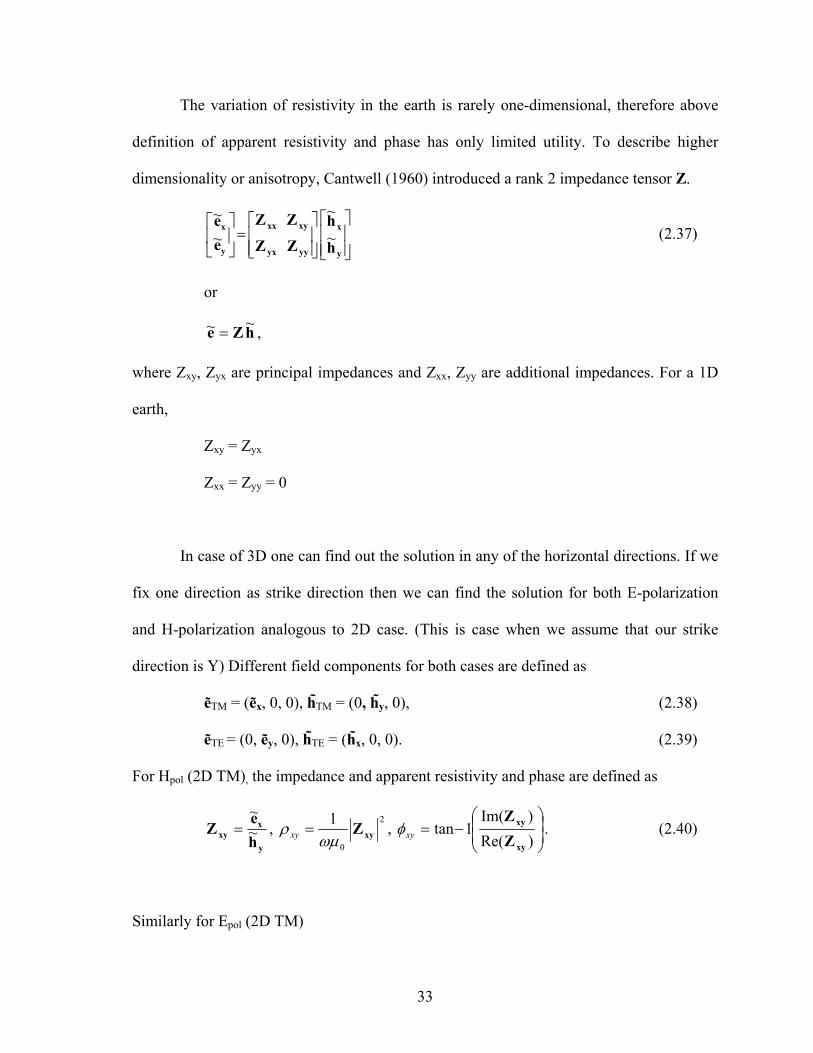
The variation of resistivity in the earth is rarely one-dimensional, therefore above

definition of apparent resistivity and phase has only limited utility. To describe higher

dimensionality or anisotropy, Cantwell (1960) introduced a rank 2 impedance tensor Z.

⎥⎥⎦

⎤

⎢⎢⎣

⎡

⎥⎥⎦

⎤

⎢⎢⎣

⎡=⎥⎦

⎤⎢⎣

⎡

y

x

yyyx

xyxx

y

x

h

hZZ

ZZee

~

~

~~

(2.37)

or

hZe ~~ = ,

where Zxy, Zyx are principal impedances and Zxx, Zyy are additional impedances. For a 1D

earth,

Zxy = Zyx

Zxx = Zyy = 0

In case of 3D one can find out the solution in any of the horizontal directions. If we

fix one direction as strike direction then we can find the solution for both E-polarization

and H-polarization analogous to 2D case. (This is case when we assume that our strike

direction is Y) Different field components for both cases are defined as

ẽTM = (ẽx, 0, 0), hTM = (0, hy, 0), (2.38)

ẽTE = (0, ẽy, 0), hTE = (hx, 0, 0). (2.39)

For Hpol (2D TM), the impedance and apparent resistivity and phase are defined as

y

xxy h

eZ ~

~= ,

2

0

1xyZ

ωµρ =xy , ⎟

⎟⎠

⎞⎜⎜⎝

⎛−=

)Re()Im(

1tanxy

xy

ZZ

xyφ . (2.40)

Similarly for Epol (2D TM)

34

x

yyx h

eZ ~

~−= ,

2

0

1yxZ

ωµρ =yx , ⎟

⎟⎠

⎞⎜⎜⎝

⎛−=

)Re()Im(

1tanyx

yx

ZZ

yxφ . (2.41)

The vector Helmholz equation with requisite boundary conditions is posed as EM

eigenvalue problem. The theory of EM problem using eigenmode is presented. Total field

formulation, secondary field formulation, derivation of h field and the response functions

such as impedance, apparent resistivity and phase are described here. The EM eigenvalue

problem can not be solved analytically because the analytical solution does not exist for

boundary value problems with arbitrary variation of resistivity. Therefore, the EM

eigenvalue problem, in its generality, can only be solved using some numerical technique.

In present work the numerical technique Finite Difference Method is used to transform the

EM eigenvalue problem (2.23) to the corresponding matrix eigenvalue problem and

Lanczos/Arnoldi methods are used to solve for the eigenvalue/eigenvectors of the matrix.

These methods are discussed in the next chapter.

35

CHAPTER 3

FINITE DIFFERENCE IMPLEMENTATION

3.1 Introduction

The EM data interpretation activity crucially depends upon the accuracy and

efficiency of the forward modeling algorithm. The analytical solutions of the governing

partial differential equation, derived from Maxwell’s equations, exist only for models with

simple geometry and resistivity variation such as layered earth, sphere, etc. Even these

analytical solutions involve complex integral or infinite series. Hence, an exact solution of

most EM problems is not computable. The only alternative is to opt for numerical

solutions.

There are two broad classes of numerical methods; Integral Equation Method (IEM)

and Differential Equation Method (DEM). Both of these classes of methods have merits

and demerits in terms of their efficiency and versatility. Preference of one method over the

other is governed by the complexity of the model and available computer resources. These

methods translate the integro-differential operator equation into a matrix equation. In IEM,

the integral operator equation is transformed to the matrix equation through quardrature

formulae. In IEM only anomalous region is modeled, resulting in a small but full

coefficient matrix. However, the popular use of IEM is restricted to only finite volume

targets buried in a simple geometry host.

For arbitrary variation of conductivity, the DEMs, like Finite Difference Method

(FDM) and Finite Element Method (FEM), are commonly used. In these methods the

whole domain of study is discretized. This results in large but grossly sparse coefficient

36

matrix. Recent advances in iterative matrix solvers, has resulted in these methods becoming

superior to IEM. In FEM, the differential operator is reduced to a matrix through functional

minimization while in FDM, it is reduced through finite difference equations. The

mathematics of FDM is easier to implement than that of FEM. In the present work, FDM is

used for 3D MT modeling.

3.2 Finite Difference Implementation

In FDM, the derivatives are approximated by the appropriate difference formula

obtained by the Taylor series expansion. For detailed description of FDM, one can refer to

standard texts like Forsythe and Wasow (1964), Hildebrand (1974), Mitchell and Griffiths

(1980), Taflove (1995). A brief account of FD formulation of EM problem follows.

The EM eigenproblem defined by equation (2.23) can be transformed using the

vector identity given in equation (2.32), to the differential equation

e(r)e(r) σλµ02 =∇− . (3.1)

This eigenproblem can be rewritten as

dvdvv v

ϕσλµϕ∫∫∫ ∫∫∫−=∇ 02 , (3.2)

where, φ denotes the scalar quantity representing any one of the three electric field

components. Using Gauss integral theorem, the left hand side of the equation (3.2) can be

transformed into surface integral equation

dsndvv s∫∫∫ ∫∫ ⋅∇=∇⋅∇ ˆ)( ϕϕ , (3.3)

This step transforms the second order partial differential equation into first order one

which is then approximated using central difference formulae.

37

For implementation of FDM to solve equation (3.1), the 3D grid discretization of a

block domain is presented in the Figure 3.1. It is discretized by straight lines parallel to the

three- coordinate axes (x-, y-, z-) in cartesian coordinates.

Figure 3.1: 3D Finite Difference grid.

3.2.1 Implementation of staggered grid

One can use either a normal grid or a staggered grid to implement FDM. In normal

grid all the six electric and magnetic field components are assigned to one node while in

staggered grid these are assigned to different points in a grid. As a result of numerical

computations, B⋅∇ is not exactly zero in case of normal grid. However, in case of

staggered grid, due to the arrangement of the electric and magnetic field values, B⋅∇ is

implicitly zero. Thus, the field values, computed using staggered grid, are less erroneous

k = nz

k = 1

i = nx

i = 1 y

x

z

z = 0

j = 1 j = ny

σ(i,j,k)

38

than those obtained using nodal grid. The staggered grid was introduced by Yee (1966) for

electrical engineering problems but is now widely used to solve the EM problems in

various disciplines.

Let the number of cells in the grid be nx, ny and nz in x-, y- and z- directions

respectively. Conductivity of the cell (i,j,k) is represented as σ(i,j,k) and its volume as

v(i,j,k) = a(i).b(j).c(k), where a(i), b(j) and c(k) are the distances between two adjacent

nodes in x-, y- and z- directions respectively (Figure 3.2). The edges of the cube are (x(i),

x(i+1)), (y(j), y(j+1)) and (z(k), z(k+1)). The cell edge centers are defined as xc(i), yc(j)

and zc(k) with

2

)1()()( ++=

ixixixc , 2

)1()()( ++=

jyjyjyc and 2

)1()()( ++=

kzkzkzc .

The distance between two adjacent midpoints are defined by ah(i), bh(j) and ch(k) in x-, y-

and z- directions respectively.

Figure 3.2: Arrangement of electric and magnetic field components on Yee’s

grid.

c(k)

b(j)

a(i)

by(i,j,k) bx(i,j,k)

ez(i,j,k)

ex(i,j,k)

ey(i,j,k)

z

x

y bz(i,j,k)

39

In Yee’s staggered grid implementation, the six field components (three electric and

three magnetic) are assigned to different points of each cell. In the current presentation

(Figure 3.2) electric field components are assigned to the centre of cell edges while

magnetic components are assigned to the centre of cell faces. In Figure 3.2, ex (i, j, k) is

defined at xc(i), y(j) , z(k) position, ey(i, j, k) at x(i), yc(j), z(k) and ez (i, j ,k) at

x(i),y(j),zc(k) respectively.

At the air-earth interface (z = 0), the grid is artificially extended to half cell height

c(1)/2, into the air and the missing values are obtained by using field continuation

algorithm given in Appendix A1 in detail. Rest of the five domain bounding surfaces are

assumed to be perfectly conducting and the homogeneous Dirichlet boundary condition i.e.

vanishing tangential component of electric eigenmodes at each surface, is imposed.

When employing FDM to solve the problem, it is better to take spatial average of

conductivity at a node (Weaver, 1976). The integration is taken over a prism centered at the

point where the electric component is evaluated to calculate the volume weighted average

conductivity of the surrounding prism. The average conductivities, ),,( kjixσ ,

),,( kjiyσ and ),,( kjizσ , correspond to eigenmode components are ),,( kjiex , ),,( kjiey

and ),,( kjiez respectively. The average conductivity ),,( kjixσ , shown in Figure 3.3, is

defined as

⎭⎬⎫

⎩⎨⎧

−−+−−−−+−−+

=)1,,()1()(1,1,()1()1(

),1,()()1(),,()()(),,(4

1),,(kjikcjbkjikcjb

kjikcjbkjikcjbkjiV

kjix

x σσσσ

σ ,

where )()()(),,( kcjbiakjiV hhx ⋅⋅= . (3.4)

40

Figure 3.3: The grid cells and associated electric (red colour) and magnetic (blue colour) components required for the FD equation of ex(i,j,k). The shaded prism is of averaged conductivity ),,( kjixσ .

The Finite Difference (FD) approximation of eigenvalue equation for xe component is

obtained from equation (3.3),

),,(e),,()(

)1,,(b),,(b)(

),1,(b),,(bx0

yyzz kjikjikc

kjikjijb

kjikjix

hh

σµ=−−

−−− . (3.5)

Here, by and bz are magnetic field components in y and z directions and these are further

FD approximated, when applying equation (2.22) into equation (2.3) as

),,(b)(

),,(e),1,(e)(

),,(e),,1(ez

xxyy kjijb

kjikjiia

kjikjiλ=

−+−

−+. (3.6)

From the two equations (3.5) and (3.6), it is clear that each electric component is

connected with only surrounding twelve electric components. Therefore, the resulting

x

y

z

ch(k)

a(i)

bh(j)

σ(i,j-1,k-

ex(i,j,k)

by(i,j,k)

by(i,j,k-

bz(i,j,k) bz(i,j-

σ(i,j,k) σ(i,j-1,k)

σ(i,j,k-1)

xσ (i,j,k)

41

coefficient matrix will be 13 diagonal matrix. The symmetry of this matrix is conserved by

the transformation;

),,(e),,(),,(e xx kjikjidkji x= , (3.7)

where the transformation factor dx(i, j, k) is

),,(),,(),,( 0 kjiVkjikjid xxx σµ= ,

with Vx(i, j, k) being volume of the prism surrounding the point (i,j,k) where field is

evaluated.

The resulting final equation for all electric field components in all the three directions is

described in Appendix A2.

3.3 Description of System Matrix

After employing finite differences representation, the algebraic equations are

assembled to form a matrix equation;

ee λ=A . (3.8)

The electric field components can be arranged in different ways. Using different

arrangements the eigenvalues and eigenvectors are not changed but the computational

efficiency may be affected. The matrix A is real, symmetric, semi-positive definite and

grossly sparse. The size of the matrix depends upon the total number of electric field

components. The numbers of three electric field components are,

number of ex components = nx (ny-1) nz,

number of ey components = (nx-1) ny nz,

number of ez components = (nx-1) (ny-1) nz.

Thus, the size of the matrix is

42

NA = Nh nz + (nx-1) (ny-1) nz. (3.9)

with Nh = nx (ny-1) nz + (nx-1) ny.

The system matrix has a maximum 13 non-zero elements in each row or column

besides the full block, due to field continuation, corresponding to the horizontal field

components at air-earth interface. This full block is of dimension Nh x Nh.

Firstly, the matrix eigenvalue problem is solved using the direct method of Singular

Value Decomposition (SVD). This method does not take into account symmetry and

sparsity and hence is not suitable for large size problems because of the explicit storage

requirement of the matrix. To check the working of eigenmode formulation, the method

was tested for half space model having resistivity10 Ω-m, discretized using a uniform grid

having 566 ×× cells in x-, y- and z-directions respectively. The resulting eigenvalues are

plotted vs. eigenvalue number in Figure 3.4.

eigenvalue number

0 100 200 300 400 500

eige

nval

ues

0

50

100

150

200

250

300

350

Figure 3.4: The eigenvalue plot for uniformly discretized half space.

43

Striking feature of the full spectrum of eigenvalues, shown in Figure 3.4, is that

about one third of the total eigenvalues are equal to zero. In fact, the number of these zero

eigenvalues is exactly equal to the number of internal nodes of the grid which is also equal

to the number of ez components, i.e. (nx-1)(ny-1)nz. These zero eigenvalues are termed

as spurious eigenvalues and corresponding eigenvectors are also termed as spurious

eigenvectors as these do not contribute to the field synthesis. Only the positive eigenvalues

contributes to the solution. The positive eigenvalues are generally simple but may be

multiple for degenerate case like, half space model. These positive eigenvalues are

bounded in a region (λmax – λmin) as given below,

The min value of eigenvalue λmin is defined as,

,12

2

2max

2

max0min ⎟⎟

⎠

⎞⎜⎜⎝

⎛+≈

zLLαπ

σµλ παπ <<2/ . (3.10)

The maximum value λmax is defined by,

,)()(

1)(

11222

min0max ⎟⎟

⎠

⎞⎜⎜⎝

⎛∆

+∆

+∆

≈zyxγ

σµλ 1>γ . (3.11)

Here, lower bound depends on the overall dimension of the model while the upper bound

depends upon grid discretization (Weidelt, 2009). Next section describes how these

spurious eigenvalues are eliminated.

3.4 Elimination of Spurious Eigenmodes

The spurious eigenvalues suggest that the system has less degree of freedom than

envisaged from the geometry. To study how these spurious modes can be eliminated, take

the divergence of the eigenvalue equation (2.23),

0))()(( 0 =−×∇×∇⋅∇ rr ee σλµ , (3.12)

44

0))(( 0 =⋅∇ reσλµ . (3.13)

There are only two possibilities;

i) either λ ≠ 0 then 0))()(( =⋅∇=⋅∇ je rrσ

ii) or λ = 0 then 0≠⋅∇ j .

In the second case, the divergence free current density condition is not satisfied. Thus, to

avoid spurious eigenmodes, the divergence free condition is enforced explicitly.

0=⋅∇ j , (3.14)

0jjj zyx =∂∂

+∂

∂+

∂∂

zyx. (3.15)

Now, applying FD to this divergence equation we get,

0)(

)1,,(j),,(j)(

),1,(j),,(j)(

),,1(j),,(j zzyyxx =−−

+−−

+−−

kckjikji

jbkjikji

iakjikji

hhh

. (3.16)

The definition of jx, jy and jz are,

),,(e),,(),,(j xx kjikjikji xσ= ,

),,(e),,(),,(j yy kjikjikji yσ= ,

),,(e),,(),,(j zz kjikjikji zσ= . (3.17)

The number of spurious eigenmodes is equal to the number of ez components, solving

above equation for ez component,

⎥⎥⎥⎥

⎦

⎤

⎢⎢⎢⎢

⎣

⎡

−−

+−−

−−−

=

)(),1,(j),,(j

)(),,1(j),,(j

),,()(

)1,,(e),,(

)1,,(),,(eyy

xx

zz

jbkjikji

iakjikji

kjikc

kjikji

kjikji

h

h

z

h

z

z

σσσ . (3.18)

Using Ohm’s law to express jx and jy in terms of ex and ey respectively we get,

45

⎥⎥⎥⎥⎥

⎦

⎤

⎢⎢⎢⎢⎢

⎣

⎡

−−−

−

+−−−

−

−−−−

=

),1,(e)(

),1,(),1,(),,(e

)(),,(),,(

),,1(e)(

),,1(),,1(),,(e

)(),,(),,(

),,(),,()(

)1,,(e),,(),,(

)1,,()1,,(),,(e

yy

xx

zz

kjiib

kjidkjikji

ibkjidkji

kjiia

kjidkjikji

iakjidkji

kjidkjikc

kjikjidkjikjidkji

kji

h

yy

h

yy

h

xx

h

xx

zz

h

zz

zz

σσ

σσ

σσσ

3.19)

For first layer corresponding to k =1, the first term in above equation is zero

because 0)1,,( =−kjizσ . Thus, each vertical component can be represented by four

horizontal components of the same layer and four components of the layer just above it.

Thus, for each vertical component a total of k⋅4 components are added to each row. This

equation is applied to all ēz components, reducing the matrix dimension to NR = NA – Nv,

Nv being the number of ez components. In the reduced matrix, the number of non-zero

elements from the direct FD coefficient matrix reduces to 9 from 13 because of

replacement of four ēz vertical components with horizontal components. This suggests a

maximum of k⋅16 replacements in general, and it leads to )12(6 −⋅ k non-zero elements in a

row of layer k.

This increase of additional elements in a row leads to loss of symmetry. Each layer

components are related to all the components of above overlying layers.

3.5 Reduced System Matrix

The reduced coefficient matrix structure is shown in Figure 3.5. The eigenvectors

have only the horizontal components. The dimension of reduced system matrix is

( ) zyxyxR nnnnnN )1()1( −+−= . The matrix is real, non-symmetric, positive definite, and

smaller in size by a factor of approximately 1/3. It is less sparse in comparison with the

original symmetric matrix. The matrix elements are stored in compressed sparse row (CSR)

46

format (Saad, 1994) because of its efficient performance for some of the standard matrix

operations.

Figure 3.5: Representation of reduced matrix structure.

After implementing the divergence correction, the final reduced matrix is obtained.

Now, the eigenmodes of this matrix are to be found using some efficient eigenmode solver.

3.6 Eigensolver for the Matrix

A variety of matrix eigensolvers such as direct, iterative and semi iterative are used

in EM problems (Sarkar et al., 1981). Direct solvers, where the complete matrix banded or

full matrix is stored, provide the solution in finite but large number of steps. In iterative

methods, on the other hand, where an initial guess is improved in a series of iterations, the

procedure can be stopped whenever the approximate solution with prescribed accuracy is

obtained. Iterative methods exploit sparsity structure of the matrix to the maximum

(Jacobs, 1981) and are therefore preferred for sparse systems. Though iterative solvers

47

score on sparsity ground, yet their use is not recommended when diagonal dominance is

not guaranteed or when the matrix is indefinite. Semi-iterative methods based on Conjugate

Gradient (CG) method are commonly used even for indefinite matrices.

When the coefficient matrix is real, positive definite and large in size, iterative

methods are widely used to obtain the eigenvalues and eigenvectors. The oldest method to

find eigenvalue iteratively is the power method. This method was first used to find the

largest eigenvalue of the system matrix. Krylov subspace projection methods are based

upon the intricate structure of the sequence of vectors naturally produced by the power

method. In Krylov methods, only product of the matrix with a vector is needed. Arnoldi

and Lanczos are popular Krylov subspace methods. Lanczos is used for symmetric

matrices while Arnoldi is used for non-symmetric matrices. Since in our eigenmode

solution of EM field problem, only a small subset of smallest eigenvalues is needed, we

have adapted the ‘ARPACK software’ subprograms based on Arnoldi method, in the

development of our eigenmode solver to find the eigenvalues.

ARPACK (Arnoldi Package) (Lehoucq et al., 1997) is a collection of FORTRAN

subroutines used to solve large eigenvalue problems. This is based on implicit restart

scheme, known as Implicit Restarted Lanczos/Arnoldi Method (IRAM/IRAM), which is

very efficient in finding a small subset of desired (either smallest or largest) number of

eigenvalues and eigenvectors of a matrix. Storage requirement are of the order of

))()(( 2kOkON +⋅ . This software is capable to determine the desired pre-specified number

of eigenvalues for largest magnitude (LM), smallest magnitude (SM), largest algebraic part

(LA) and smallest algebraic part (SA). To obtain the desired subset the implicit restarted

scheme is presented in the next section.

48

3.6.1 Implicitly restarted Lanczos/Arnoldi method

Lanczos/Arnoldi method is a Krylov subspace based method. A basis of Krylov

subspace can be obtained from any arbitrary starting vector (V1) and its repeated product

with the system matrix A. The Krylov basis vectors not being orthogonal, are

orthogonalized and the orthogonalized basis vectors serve as Lanczos/Arnoldi vectors.

Lanczos/Arnoldi method was used to solve for all eigenvalues and eigenvectors of a

symmetric/nonsymmetric matrix using the relation

rVHAV += , (3.20)

where A is the coefficient matrix, V is the matrix of Lanczos/Arnoldi vectors of dimension

N column-wise, H is a symmetric tri-diagonal/upper Heisenberg matrix and r is the

residual vector. The Matrix A is of NN× and the vector r is an N dimensional vector.

Complete eigenanalysis of the tridiagonal/upper Hessenberg matrix H need be performed.

This, in turn, leads to eigenvectors of matrix A. Theoretically, r should be zero but in finite

precision arithmetic it has a prescribed very small value.

Presently, Lanczos/Arnoldi Method is widely used to find a desired subset of

eigenvalues as described by Sorensen (1992). In the present case, the interest is in M

smallest eigenvalues and corresponding eigenvectors. After the generation of M

Lanczos/Arnoldi vectors, the residual vector has a finite value. To find M smallest

eigenvalues and corresponding eigenvectors, we have to generate a subspace with M+P

Lanczos/Arnoldi vectors as given below

TPMPMPMPMPM erHVAV +++++ += . (3.21)

In this case V matrix is of the order of N×(M+P) and H matrix is of the order of

(M+P)×(M+P). Eigenanalysis of this smaller dimensional matrix H is performed rather

49

than full N×N matrix. The eigenvalues obtained from this M+P factorization reflects

characteristics of full spectrum of N eigenvalues. We arrange M+P eigenvalues in

increasing order so that last P largest eigenvalues becomes unwanted ones. These P values

are used as shifts to update the first M values via QR iterations. In this updating process

Lanczos/Arnoldi vectors are forced to belong to the subspace corresponding to smallest

eigenvalues and the residual vector rM+P becomes very small iteratively. This technique is

known as Implicit Restart Techinque. It is recommended that P be greater than M. There

are two modes to find the subset of eigenvalues defined as ‘regular mode’ and ‘shift and

invert mode’ as discussed below.

3.6.1.1 Regular mode

In regular mode, one deals with the problem

xAx λ= . (3.22)

In this mode only product of the matrix with a vector is needed. Arnoldi method converges

faster for larger magnitude eigenvalues; therefore to calculate smallest eigenvalues with

SM or SA it takes longer time.

3.6.1.2 Shift and invert mode

In shift and invert mode, the dealing equation is

ξλννξ

−==− − 1,)( 1 xxIA . (3.23)

The eigenvalues converges near to applied shift ‘ξ’. This method converges faster

when determining the smallest eigenvalues. The main disadvantage of implementing this

mode is that one must provide a matrix solver, either direct or iterative, to obtain the term

(A-ξI)-1x.

50

Any one of the conjugate gradient based methods can be used to solve for the

product (A-ξI)-1x. There are different variants of conjugate gradient methods such as

Conjugate Gradient (CG), Bi-Conjugate Gradient (BiCG) and Bi-Conjugate Gradient

Stabilized (BiCGStab) methods. To increase efficiency of these methods, different

preconditioners such as Jacobi or incomplete factorization methods are also used.

Incomplete factorization method ILU (0) means that during LU factorization there is zero

fill in. Van der Vorst (2003) suggested that BiCGStab with ILU(0) gives better results. The

number of iterations needed to solve a matrix equation by various methods using the

preconditioner ILU (0), are given in Table 3.1. The matrix was of order 5050× .

Table 3.1: Comparison of different methods with preconditioners for best invert matrix solver.

Method Number of iterations

CG 30

BiCG 20

BiCGStab 15

CG + ILU(0) 12

BiCGStab + ILU(0) 9

3.7 Synthesis of Full Eigenvector

The eigenvectors of the reduced matrix obtained using IRAM are orthogonal to

each other. As the reduced eigenvectors comprise only the horizontal components, these

have dimension NR. The eigenvectors must be transformed into full eigenvectors for use in

51

field synthesis. The remaining components of the eigenvectors are obtained by using

spurious eigenvector relation (3.19). The ez components are appended to the reduced

eigenvector components. A good feature is that these full eigenvectors are also numerically

orthogonal. Hence, there is no need to orthogonalize these full eigenvectors again

explicitly. However, these eigenvectors should follow the sigma orthogonality relation,

ln1

)()(ˆ)(ˆ)( δσ =∑=

mVmmmAN

mnl ee . (3.24)

This condition yields a scaling factor nη , given in Appendix A2, which provides the final

sigma orthogonalized eigenvectors as,

nn ee ⋅= nηˆ , (3.23)

where en are back transformed from ne using the transformation relation (3.13).

This completes the discussion of implementation of Finite Difference for the

solution of eigenmodes. These eigenmodes are used to solve for the superposition

coefficients using equation (2.33). Secondary field values are then solved using equation

(2.26) and finally equation (2.29) gives the total field values, ẽT. These field values are next

used to derive the magnetic field h and the response functions: impedance, apparent

resistivity and phase. In next chapter, developmental details of the algorithms MT_2D_EA

and MT_3D_EA are discussed.

53

CHAPTER 4

DEVELOPMEMNT AND DETAILS OF ALGORITHM

4.1 Introduction

We started with the development of 2D algorithm MT_2D_EA and finally

developed the 3D algorithm MT_3D_EA. In both these algorithms Finite Difference

Method (FDM) is used to obtain the discretized EM eigenvalue problem. The eigenmodes

of the corresponding coefficient matrix, obtained using Lanczos/Arnoldi method, are then

used to synthesize the electric field vector which, in turn, was used to obtain the magnetic

field vector and the derived MT response functions impedance, apparent resistivity and

phase. The sequence of development, highlighting the difficulties faced and the manner in

which these were overcome, is presented below.

4.2 Sequence of Development

The present study was spanned over a period of about five years. In this period 1D,

2D and 3D modeling algorithms for magnetotelluric data were developed. In this section,

the different versions of algorithm are presented. It may be stressed here that MT_2D_EA

development took only 10% of the time spent on the development of MT_3D_EA. This

was so because in the 3D case, bulk of the time was spent in overcoming the problems

resulting from coarseness of the grid used. Use of a coarse grid became necessary because

of the limitation on size of the problem imposed by the available PC or work station. As a

byproduct, this study has led to a better understanding of the effect of coarseness of the

grid on MT response.

54

4.2.1 Development of MT_2D_EA algorithm

Initially, the 2D algorithm was developed using the same methodology as was to be

used in 3D case i.e. eigenmode analysis using FDM. In the first development, the Dirichlet

boundary condition was applied on all the four domain boundaries i.e. the two horizontal

and the two vertical sides. The problem was solved only for internal nodes using total field

formulation. The results were satisfactory at the centre of the model but these were

somewhat anomalous near the vertical domain boundaries. The problem was circumvented

by using autogrid and more appropriate boundary conditions. We replaced the manual grid

with an autogrid generated scheme employing the skin-depth EM field decay criterion.

Further, the application of integral boundary condition at the air earth interface and of

asymptotic boundary condition at the vertical sides provided the accurate results even at the

vertical boundaries of the domain. Since in MT formulation, the derived observables:

impedance, apparent resistivity and phase, depend on the ratio of the components of E and

H field values, we verified that for both E and H field boundary conditions the results are

same. Prior to this conclusion achieved, all the eigenmodes were computed and then used

to synthesize the electric field.

Sufficiently large time and memory is required for the solution of all eigenmodes.

In the expression of the superposition coefficient, in equation (2.27) or (2.32), the

eigenvalue appears in the denominator and thus smallest eigenvalues dominate in the field

synthesis. This observation suggested that use of only a small subset of smallest

eigenvalues and corresponding eigenvectors may accurately synthesize the electric field

values and thereby significantly reduce the computational time. For implementation of this

step, the Implicitly Restarted Lanczos Method (IRLM) is used. This implementation

55

produces numerically accurate field values for 5% of eigenmodes in one fourth of the

computational time needed for all eigenmodes.

4.2.2 Development of MT_3D_EA algorithm

In the case of 3D, taking cue from the experience of 2D algorithm, right from the

beginning we implemented the integral boundary condition (IBC) at air earth interface.

Following the formulation given in chapter 3, first the coefficient matrix (equation

(3.8)) was generated for all electric field components. The resulting matrix was a 13-

diagonal symmetric matrix. We used Singular Value Decomposition (SVD) to solve for the

eigenvalues and eigenvectors of this matrix. About one third (exactly equal to no. of

vertical electric field components) of the total eigenvalues of this symmetric matrix was

found to be zero. These zero eigenvalues and corresponding eigenvectors are termed as

‘spurious’ and these are not used for field synthesis. The secondary field values are

obtained without these spurious eigenmodes. Finally, the derived magnetic field and

response functions are calculated using the electric field values.

The zero eigenvalues create difficulty in getting the smallest non-zero eigenvalues.

This problem was resolved by using the current divergence equation (3.18) to eliminate the

vertical electric field components by expressing these in terms of the horizontal

components. However, in this process, the structure of resulting coefficient matrix is

changed from symmetric to non-symmetric. Due to this we were unable to use the IRLM

which is applicable only to symmetric matrices. Implicitly Restarted Arnoldi Method

(IRAM) is used for non-symmetric matrices. In IRAM to obtain smallest eigenmodes Bi-

CGStab (Bi- Congugate Gradient Stabilizer) with preconditioner ILU(0) is used. Using the

IRAM, we observed that the convergence is achieved after two iterations itself. This

56

process did result in the convergence of eigenvalues. However, inspite of the fact that the

remainder vector becomes null, the eigenvectors did not converge. This problem gets

resolved, if in the next updating of eigenmodes, a non null vector (that is orthogonal to the

previous eigenvectors) is used. These eigenmodes are finally used for field synthesis and

response computations.

4.3 Salient Features of MT_3D_EA Algorithm

Besides the eigensolvers, various other steps are taken to enhance the efficiency and

versatility of the algorithm MT_3D_EA. Since the algorithm has a compact modular

structure, a subroutine can be plugged in or taken out easily without affecting the

remaining program. The features to enhance versatility or efficiency are discussed below.

4.3.1 Response functions

The algorithm is presently developed to get the responses for magnetotelluric

profiling. The responses are computed at the surface for a single frequency. The algorithm

can compute response functions like impedance, apparent resistivity and phase, for both the

modes, 2D-TE and 2D-TM given by equations (2.41) and (2.40) respectively. The choice

of response modes is controlled by the counter mode_type. The response functions

impedance and apparent resistivity and phase are computed in subroutine output_3D.

4.3.2 Source term

The program is so structured that the computations are carried out in terms of

secondary fields. Later on, for total field computations, the primary fields are added to

these secondary fields. Thus, in order to incorporate the source effect, only a subroutine

computing the responses of primary layered earth model in the presence of given source, is

57

added in lieu of the existing subroutines eigenmode_1D and output_1D which compute the

1D field due to a plane wave source.

4.3.3 BiCGStab method

Arnoldi method converges better in invert mode when evaluating the smallest

eigenvalue. In invert mode, the matrix solver Bi Conjugate Gradient Stabilized (BiCGStab)

is used because with appropriate preconditioner it provides the solution in optimal time.

4.3.4 Multi-frequency response

In the proposed approach, eigenmodes are independent of source or frequency and

these depends only on the model characteristics. In conventional FDM algorithms, the

program has to be re-run to generate the response for each frequency, while in our

approach, once the eigenmodes are evaluated, the responses for different frequencies can

be easily computed in negligible computer time.

4.4 Description of MT_3D_EA Algorithm

The algorithm, MT_3D_EA, employs FDM for solving the EM eigenproblem to

compute the 3D MT responses. The algorithm comprises 11005 lines and 60 subroutines. It

employs 4 complex arrays, 75 real arrays, 14 real variables and 24 integer variables. It

works in double precision arithmetic. In order to control dimension overflows, various

checks with error and stop messages are inserted in the program. The arrays are initialized

and reused to optimize the memory requirement. The description and salient features are

highlighted in the Figure 4.1.

Total seven I/O units are opened in the program. The parameters and data controls

are read from the input file. Two scratch files are used for buffer storage. The remaining

58

four output files are used for different outputs helpful in analyzing the results. Sample

input/output files are given in the Appendix A4.

Figure 4.1: Algorithm in nutshell.

4.5 Structure of MT_3D_EA Algorithm

The main module of the algorithm MT_3D_EA provides the infrastructure and runs

the controls. In the main program the control parameters are defined, input and output files

are opened and the subprograms are called as shown in Figure 4.2. Input data and other

Basic Algorithm Statistics

MT_3DEA - 11005 Lines

Main program - 158 Lines

Subroutines - 10847 Lines

60 (40+20*)

* Adapted from other program

Methodology

Finite Difference Method to transform the EM eigenproblem to matrix

eigenproblem

Eigenmode Formulation to express the electric field components as a linear

superposition of eigenvectors of the EM eigenproblem

Bi-CGStab with ILU(0) Preconditioner to implement the shift and invert mode of

IRAM efficiently

Salient Features

Integral boundary condition at the air-earth interface

IRLM/IRAM for eigenproblem solution

Very fast Multi-frequency response computation using eigenmodes

59

parameters are read in the subroutine input. A list of various subprograms highlighting their

purpose and other details is given in Table A3.3 of Appendix A3.

The grid data can be read in two ways either as a manually generated grid or as a

logarithmically generated grid. The control parameters irx, iry and irz respectively control

the grid choice in x-, y- and z-directions. The logarithmic grids are computed in subroutine

grid. The resistivity or conductivity is read for the half space and for the anomalous prisms

and finally stored in 3D arrays sx, sy and sz. Calculations of the elements of coefficient

matrix, for all electric field components, are carried out in subroutine weight. Subroutine

weight_ez is used for calculations for updating the elements corresponding to the horizontal

components of coefficient matrix in the reduced matrix case where the ez components are

replaced in terms of horizontal components ex and ey (equation (3.18)). Integral boundary

condition is implemented in subroutines conti1, conti2, conti3 and conti4 depending upon

the uniformity and non-uniformity of grids in horizontal directions. The starting vector is

initialized in subroutine init.

The subroutine eigenmode_1D is used for 1D layered model coefficient matrix and

eigenmode computations and the subroutine output_1D generates primary field values for

given frequency. 3D eigenmodes are computed in subroutine eigenmode_3D. These

eigenmodes are used in subroutine output_3D for response function computations. The

responses are obtained, in subroutine output_3D, by computing (i) the superposition

coefficients using equation (2.33), (ii) the secondary field values using equation (2.26), (iii)

the total field values using equation (2.29), and (iv) the response functions impedance and

apparent resistivity and phase using equations (2.40) and (2.41) respectively.

60

Figure 4.2: Flow chart of main program.

61

The subroutines output_1D and output_3D are recalled when the responses for multi-

frequencies are to be computed.

Bulk of the computer time is consumed in eigenmode computations carried out in

the subroutine eigenmode_3D whose flow chart is shown in Figure 4.3. It calls subroutine

eigenstep to generate the Hessenberg matrix of Arnoldi formulation element and new

Lanczos/Arnoldi vector (equation (3.20)). eigenstep implements the updating of

eigenmodes using equation (3.21). This subroutine eigenstep is called twice if a subset ‘k’

of eigenmodes is needed, first for computing k components and secondly for computing p

components (p>k). Eigenvalues and eigenvectors are solved in subroutine dlahqr. The

eigenvalues of the computed Hessenberg matrix are ordered increasingly and last p

eigenvalues are applied as shift to update first k eigenvalues in subroutine dnapps, adapted

from ARPACK. During the iterative process last p values are discarded after dnapps and

eigenstep is recalled for p component computation. This iterative process stops after

reaching a threshold value lanc_tolr. The outcome eigenvectors contains only ex and ey

components and remaining ez components are calculated in subroutine get_ez to constitute

full eigenvector.

Subroutine bicgstab is used in invert mode of IRAM (equation (3.23)) to solve a

subset of eigenmodes as desired in eigenstep for subset of eigenmodes computation as

shown in Figure 4.4. Subroutine ae1 is used for all eigenmode computation. In this

subprogram Arnoldi steps are applied twice to get numerically orthogonal eigenvectors.

Finally Hessenberg matrix is the outcome of this subprogram.

62

Figure 4.3: Flow chart of EIGENMODE_3D subprogram.

63

Figure 4.4: Flow chart of EIGENSTEP subprogram.

64

The control parameters and their purpose and numerical value for different options

are listed in Table A3.1 of Appendix A3. The grid parameters and other run environment

parameters used in different subprograms are described in Table A3.2 of Appendix A3.

The description of development of algorithm is completed. The results of experiments

performed for checking and validation of MT_2D_EA and MT_3D_EA are presented in

the following chapter.

65

CHAPTER 5

RESULTS AND DISCUSSION

After developing the requisite software it is natural to establish its efficiency and

accuracy. The accuracy is established by performing various consistency design

experiments and by reproducing the analytical results and the numerical results published

in literature. The development of 3D algorithm was preceded by the developments of 1D

and 2D codes. Therefore, first the 1D and 2D versions were tested and there after the 3D

version. However, only the comparison for the responses of 2D and 3D models is

discussed.

5.1 2D Experiments

The best check of any algorithm is the reproduction of established published results.

Two 2D models were taken from COMMEMI (Comparison Of Modeling Methods for

Electro-Magnetic Induction) paper (Zhdanov et al., 1997), one simple and other complex

one. In COMMEMI paper authors describe the results of different algorithms based on

Finite Difference, Finite Element and Integral Equation Methods for the same models for

confidence. The comparison is presented here for electric field and apparent resistivity

values only.

5.1.1 Simple model

The simple model, (2D-1) in the COMMEMI paper, is reproduced in Figure 5.1(a).

It comprises a symmetrical rectangular insert embedded in homogeneous half space. The

resistivity of the inserted block is 0.5 Ω-m while that of the half space is 100 Ω-m.

66

Figure 5.1: (a) Simple model (Model 2D-1 of COMMEMI, distance in km and resistivity in Ω-m), (b) eigenvalue plot; Comparison of COMMEMI (Zhdanov et al., 1997) and MT_2D_EA at 0.1s (c) electric field and (d) apparent resistivities.

Eigenvalue number

0 500 1000 1500 2000 2500 3000

Eig

enva

lues

1e-1

1e+0

1e+1

1e+2

1e+3

1e+4

1e+5

1e+6

1e+7(b)

Distance (km)

-6 -4 -2 0 2 4 6

Rea

l e-fi

eld

(v/m

)

0.3

0.4

0.5

0.6

0.7

0.8

0.9

1.0

1.1

COMMEMIMT_2D_EA

(c)

Distance (km)

-6 -4 -2 0 2 4 6

App

. res

. (Ω

-m)

1

10

100

1000COMMEMIMT_2D_EA

(d)

Ω-m

Ω-m

(km)

Dep

th (k

m)

(a)

67

The block, placed at a depth of 250 m from the earth surface, has a width of 1 km and

thickness 2 km. The response is computed at a period 0.1s. In Figure 5.1(b) the eigenvalue

plot for the model is presented and in Figure 5.1(c) and 5.1(d) respectively electric field

and apparent resistivity responses are compared with the average values given in the

COMMEMI paper. The RMS error between the two responses is 0.01.

5.1.2 Complex model

The complex model, (2D-4) of Zhdanov’s paper, is given in Figure 5.2(a). It

consists of different blocks with resistivities varying from 2.5 Ω-m to 1000 Ω-m and with

different widths and thicknesses. In the paper, they observed that the error is minimum at

1s. They also stated that due to the secondary field calculations, the error in apparent

resistivities varies in the range 5-10%. We are also using secondary field formulation, so

we compared the responses at the same period. The eigenvalue plot for the complex model

is given in Figure 5.2(b). The response of this model is compared in Figure 5.2(c). Again

comparison is with the average values published in the paper. The RMS error in apparent

resistivity is 0.06 or 6%, which is in the acceptance limits. We have observed that our

results are closer to the Integral Equation Method results.

After having a good response from the 2D modeling algorithm, we moved on to

study the performance of 3D algorithm. In case of 3D, due to limited computer facility, a

severe limitation on the number of grid points was imposed and we were able to run

models with very coarse grids. The effects of coarse grid led us to overcome several

spurious numerical problems. To test the algorithm, several tests are performed as

described below.

68

Figure 5.2: (a) Complex model (Model 2D-4 of COMMEMI, distances in km and resistivity in Ω-m), (b) eigenvalue plot and (c) comparison between apparent resitivities of COMMEMI and MT_2D_EA at 1s.

Eigenvalue number

0 1000 2000 3000 4000

Eig

enva

lues

1e-1

1e+0

1e+1

1e+2

1e+3

1e+4

1e+5

1e+6

(b)

Distance (km)

-12 -10 -8 -6 -4 -2 0 2 4 6

App

. res

. (Ω

-m)

1

10

100

COMMEMIMT_2D_EA

(c)

(a)

Ω-m

Ω-m

Ω-m

Ω-m

Ω-m

(km)

Dep

th (k

m)

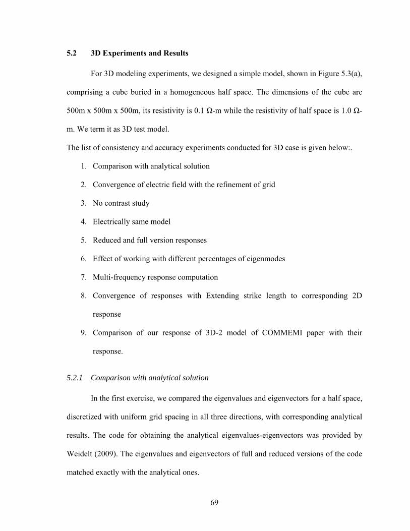
69

5.2 3D Experiments and Results

For 3D modeling experiments, we designed a simple model, shown in Figure 5.3(a),

comprising a cube buried in a homogeneous half space. The dimensions of the cube are

500m x 500m x 500m, its resistivity is 0.1 Ω-m while the resistivity of half space is 1.0 Ω-

m. We term it as 3D test model.

The list of consistency and accuracy experiments conducted for 3D case is given below:.

1. Comparison with analytical solution

2. Convergence of electric field with the refinement of grid

3. No contrast study

4. Electrically same model

5. Reduced and full version responses

6. Effect of working with different percentages of eigenmodes

7. Multi-frequency response computation

8. Convergence of responses with Extending strike length to corresponding 2D

response

9. Comparison of our response of 3D-2 model of COMMEMI paper with their

response.

5.2.1 Comparison with analytical solution

In the first exercise, we compared the eigenvalues and eigenvectors for a half space,

discretized with uniform grid spacing in all three directions, with corresponding analytical

results. The code for obtaining the analytical eigenvalues-eigenvectors was provided by

Weidelt (2009). The eigenvalues and eigenvectors of full and reduced versions of the code

matched exactly with the analytical ones.

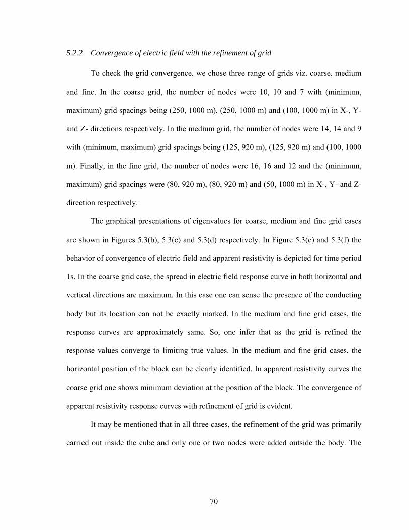
70

5.2.2 Convergence of electric field with the refinement of grid

To check the grid convergence, we chose three range of grids viz. coarse, medium

and fine. In the coarse grid, the number of nodes were 10, 10 and 7 with (minimum,

maximum) grid spacings being (250, 1000 m), (250, 1000 m) and (100, 1000 m) in X-, Y-

and Z- directions respectively. In the medium grid, the number of nodes were 14, 14 and 9

with (minimum, maximum) grid spacings being (125, 920 m), (125, 920 m) and (100, 1000

m). Finally, in the fine grid, the number of nodes were 16, 16 and 12 and the (minimum,

maximum) grid spacings were (80, 920 m), (80, 920 m) and (50, 1000 m) in X-, Y- and Z-

direction respectively.

The graphical presentations of eigenvalues for coarse, medium and fine grid cases

are shown in Figures 5.3(b), 5.3(c) and 5.3(d) respectively. In Figure 5.3(e) and 5.3(f) the

behavior of convergence of electric field and apparent resistivity is depicted for time period

1s. In the coarse grid case, the spread in electric field response curve in both horizontal and

vertical directions are maximum. In this case one can sense the presence of the conducting

body but its location can not be exactly marked. In the medium and fine grid cases, the

response curves are approximately same. So, one infer that as the grid is refined the

response values converge to limiting true values. In the medium and fine grid cases, the

horizontal position of the block can be clearly identified. In apparent resistivity curves the

coarse grid one shows minimum deviation at the position of the block. The convergence of

apparent resistivity response curves with refinement of grid is evident.

It may be mentioned that in all three cases, the refinement of the grid was primarily

carried out inside the cube and only one or two nodes were added outside the body. The

71

RMS errors of coarse and medium grid with respect to fine grid are 0.045 and 0.006

respectively.

Eigenvalue number

0 200 400 600 800 1000 1200 1400E

igen

valu

es1e-1

1e+0

1e+1

1e+2

1e+3

(b)

Eigenvalue number

0 500 1000 1500 2000 2500 3000 3500

Eige

nval

ues

1e-1

1e+0

1e+1

1e+2

1e+3

1e+4

(c)

Eigenvalue number

0 1000 2000 3000 4000 5000 6000 7000

Eige

nval

ues

1e-1

1e+0

1e+1

1e+2

1e+3

1e+4

(d)

Figure 5.3: (a) 3D Test model (distances in km); Eigenvalue plot (b) coarse grid, (c) medium grid, (d) fine grid,

1 Ω-m

0.1 Ω-m

2.25 2.5 2.75

2.75

2.25 2.5

0.10

0.60

X

Y

Z

(a) (km)

(km)

Dep

th (k

m)

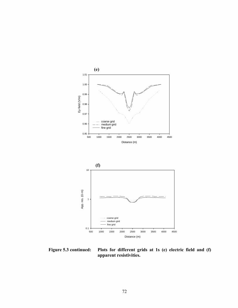
72

Figure 5.3 continued: Plots for different grids at 1s (e) electric field and (f) apparent resistivities.

Distance (m)

500 1000 1500 2000 2500 3000 3500 4000 4500

App

. res

. (Ω

-m)

0.1

1

10

coarse gridmedium gridfine grid

(f)

fine grid

Distance (m)

500 1000 1500 2000 2500 3000 3500 4000 4500

Ey-fi

eld

(V/m

)

0.95

0.96

0.97

0.98

0.99

1.00

1.01

medium gridcoarse grid

(e)

73

5.2.3 No contrast study

Another test conducted on the algorithm is to verify the convergence of a buried

target response to that of half space when the resistivity of block is taken approximately

equal to that of half space. The resistivity of block is modified to 0.9 Ω-m for this

experiment. The electric field and impedances are computed and found to be almost

identical to that of half space.

5.2.4 Electrically similar models

Next experiment is performed on electrically similar models to check the

consistency. The electrically similar model of 3D test model is 0.05 Ω-m insert in a 0.5 Ω-

m half space with same dimensions at time period 2.0s. Theoretically both models should

produce the same results. The behavior of electric field and apparent resistivity

corresponding to 2D TE and 2D TM are shown in Figures 5.4(a), 5.4(b) and Figures 5.4(c),

5.4(d) respectively. These responses also match with each other exactly. Thus it can be

concluded that the algorithm is producing consistent results.

Distance (m)

500 1000 1500 2000 2500 3000 3500 4000 4500

App.

res.

(Ω-m

)

1

0.1 ohm-m in 1.0 ohm-m at 1s0.05 ohm-m in 0.5 ohm-m at 2s

(b)

Distance (m)

500 1000 1500 2000 2500 3000 3500 4000 4500

Ey-fi

eld

(v/m

)

0.95

0.96

0.97

0.98

0.99

1.00

1.010.1 ohm-m in 1.0 ohm-m at 1s0.05 ohm-m in 0.5 ohm-m at 2s

(a)

Figure 5.4: Plots corresponding to 2D TE mode for electrically similar models (a) real Ey field, (b) apparent resistivities,

74

5.2.5 Reduced and full version

Eventually in the final algorithm, we are using the reduced version and generating

full eigenvectors from the reduced eigenvectors. To check the effect of numerical errors in

the full eigenvectors obtained from reduced eigenvectors, we compared the response of

reduced version with the response computed using the full version. The response is

compared for both the modes; one is corresponding to 2D TE as shown in Figures 5.5(a),

5.5(b) and another corresponding to 2D TM as shown in Figures 5.5(c), 5.5(d). The

comparison is given here for electric field and apparent resistivity values. These curves

match exactly with each other. This means the reduced version is working accurately.

Figure 5.4 continued: Plots corresponding to 2D TM mode for electrically similar models (c) Re Ex field and (d) apparent resistivities.

Distance (m)

0 1000 2000 3000 4000 5000

App.

res.

(Ω-m

)

1

0.1 ohm-m in 1.0 ohm-m at 1s0.05 ohm-m in 0.5 ohm-m at 2s

(d)

Distance (m)

0 1000 2000 3000 4000 5000

Ex-

field

(v/m

)

0.90

0.92

0.94

0.96

0.98

1.00

1.020.1 ohm-m in 1.0 ohm-m at 1s0.05 ohm-m in 0.5 ohm-m at 2s

(c)

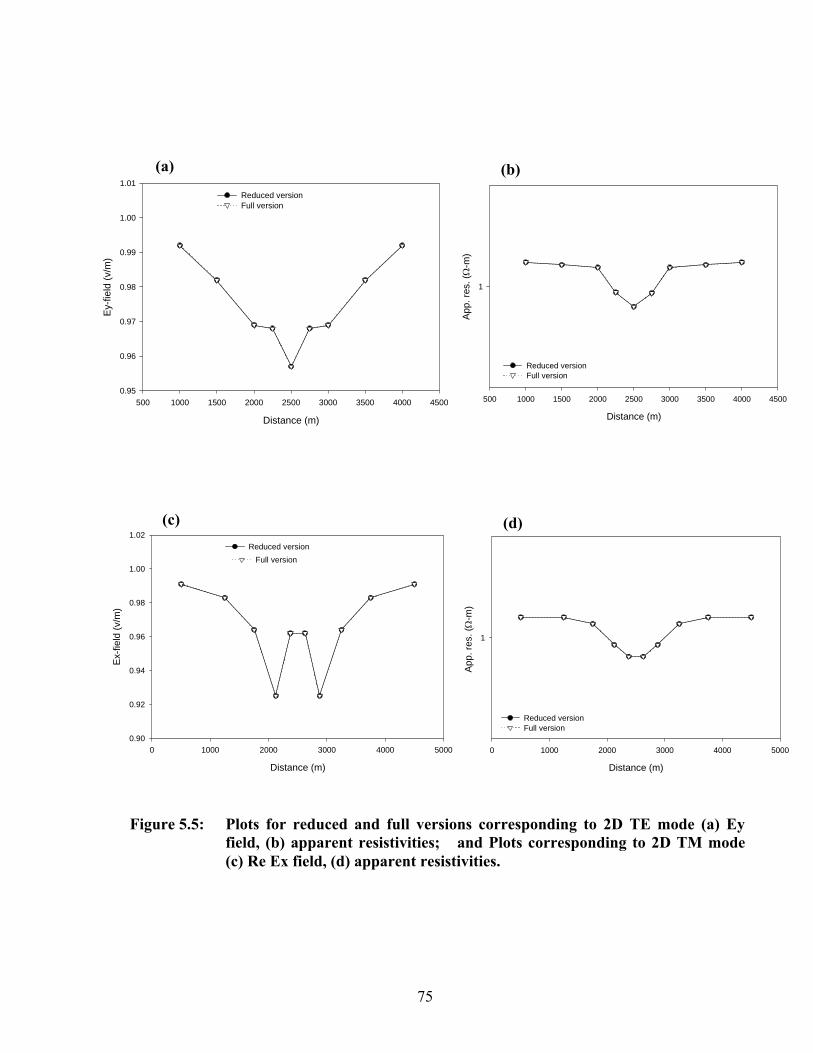
75

Figure 5.5: Plots for reduced and full versions corresponding to 2D TE mode (a) Ey field, (b) apparent resistivities; and Plots corresponding to 2D TM mode (c) Re Ex field, (d) apparent resistivities.

Distance (m)

0 1000 2000 3000 4000 5000

App.

res.

(Ω-m

)

1

Reduced versionFull version

(d)

Distance (m)

0 1000 2000 3000 4000 5000

Ex-

field

(v/m

)

0.90

0.92

0.94

0.96

0.98

1.00

1.02Reduced version

Full version

(c)

Distance (m)

500 1000 1500 2000 2500 3000 3500 4000 4500

App.

res.

(Ω-m

)

1

Reduced versionFull version

(b)

Distance (m)

500 1000 1500 2000 2500 3000 3500 4000 4500

Ey-fi

eld

(v/m

)

0.95

0.96

0.97

0.98

0.99

1.00

1.01Reduced versionFull version

(a)

76

5.2.6 Effect of working with different percentage of eigenmodes

As discussed in the chapter 2, the eigenvalues appear in the denominator of the

expression of superposition coefficient (equation (2.32)). So, in field synthesis, maximum

contribution comes from the smallest eigenvalues. The present experiment is designed to

know how many eigenvalues and corresponding eigenvectors are sufficient for numerically

accurate response. In view of limited computer resources, we chose the coarse grid model

so that we can also understand the effect of coarseness on the responses with different

percentages of eigenmodes. In this experiment the percentage of eigenmodes taken are 5,

10, 15 and 20. For these four percentage cases, the real and imaginary parts of electric field

are compared with all eigenmode response in Figures 5.6(a) and 5.6(b) respectively.

Distance (m)

500 1000 1500 2000 2500 3000 3500 4000 4500

Re

Ey-fi

eld

(v/m

)

0.95

0.96

0.97

0.98

0.99

1.00

All eigenmodes20% eigenmodes15% eigenmodes10% eigenmodes5% eigenmodes

(a)

Figure 5.6: Electric field plots for different percentages of eigenmodes (a) real part and (b) imaginary part.

Distance (m)

500 1000 1500 2000 2500 3000 3500 4000 4500

Im E

y-fie

ld (v

/m)

-0.08

-0.06

-0.04

-0.02

0.00

All eigenmodes20% eigenmodes15% eigenmodes10% eigenmodes5% eigenmodes

(b)

77

In both the plots, the maximum spread is observed for 5% and the responses

converge towards all eigenmodes response as percentage of eigenmodes increases from 5%

to 20%. The RMS errors for different percentage of eigenmodes with respect to all

eigenmodes are described in Table 5.1. This spread behavior is not expected, so we

conducted the same experiment on 2D version of this 3D test model termed as 2D test

model.

Table 5.1: RMS errors for different percentage of eigenmodes in case of 3D.

Percentage of eigenmodes Real e-field Imag e-field

5 0.0823 0.0851

10 0.0811 0.082

15 0.0798 0.08

20 0.0565 0.0583

In case of 2D, two grids are chosen to check the effect of coarseness with different

percentage, (i) the same coarse grid as used in 3D test model and (ii) the grid generated by

the auto grid generator, based on skin depth criterion. Figure 5.7(a) shows the 2D test

Model. Figures 5.7(b) and 5.7(c) show the eigenvalue curves for auto and coarse grids. In

auto grid the curve rises steeply while in the case of coarse grid the steepness is much less.

Figures 5.7(d) and 5.7(e) present the electric field and apparent resistivity responses for

auto grid while Figures 5.7(f) and 5.7(g) present the same responses for coarse grid.

78

Eigenvalue number

0 20 40 60 80 100 120 140 160 180 200

Eige

nval

ues

10-1

100

101

102

103

104

(c)

Eigenvalue number

0 200 400 600 800 1000 1200

Eig

enva

lues

10-1

100

101

102

103

104

105

(b)

Figure 5.7: (a) 2D Test model (distances in km); Eigenvalue plot (b) skin-depth based grid, (c) coarse grid,

1.0 Ω-m

0.1 Ω-m

2.25 Y

0.1

0.6

Z

2.50 2.75 (a) (km) D

epth

(km

)

79

Figure 5.7 continued: Plots for different percentage of eigenmodes; For skin depth based grid (d) Re-electric field and (e) apparent resistivities and for coarse grid (f) Re-electric field, (g) apparent resistivity.

Distance (m)

0 1000 2000 3000 4000 5000

Re

Ey-

field

(v/m

)

0.5

0.6

0.7

0.8

0.9

1.0

1.1

All eigenmodes20% eigenmodes15% eigenmodes10% eigemodes5% eigenmodes

(f)

Distance (m)

0 500 1000 1500 2000 2500 3000 3500 4000 4500 5000

Re

Ey-fi

eld

(v/m

)

0.5

0.6

0.7

0.8

0.9

1.0

1.1

all eigenvalues20% eigenvalues15% eigenvalues10% eigenvalues5% eigenvalues

Distance (m)

0 500 1000 1500 2000 2500 3000 3500 4000 4500 5000

App.

res.

(Ω-m

)

0.1

1

10

all eigenvalues20% eigenvalues15% eigenvalues10% eigenvalues5% eigenvalues

(d) (e)

Distance (m)

500 1000 1500 2000 2500 3000 3500 4000 4500

App

res

(ohm

-m)

0.1

1

10

All eigenmodes20% eigenmodes15% eigenmodes10% eigenmodes5% eigenmodes

App

. res

. (Ω

-m)

(g)

80

In auto grid case, the response curves for the four percentage cases match well with

the all eigenmode case, even 5% of eigenmodes are sufficient for accurate field synthesis.

For the coarse 2D grid, a spread behavior similar to that in 3D case is observed. However,

with increasing percentage values, the responses do converge to that for all eigenmodes.

From this exercise we conclude that auto grids provide accurate field values even for small

percentage of eigenmodes.

We also conducted the experiment to observe the effect of different percentages of

eigenmodes on the response of a resistive block model. For this purpose the model

described as 2D-3 in COMMEMI report is considered. In this model the resistive and

conductive blocks are placed at the surface. The model is shown in Figure 5.8(a) and the

corresponding eigenvalue plot is presented in Figure 5.8(b).

Eigenvalue number

0 500 1000 1500 2000 2500 3000

Eig

enva

lues

1e-4

1e-3

1e-2

1e-1

1e+0

1e+1

1e+2

1e+3

1e+4

1e+5

(b)

Figure 5.8: (a) 2D-3 model of COMMEMI, (b) eigenvalue plot,

(a)

(km)

Ω-m

Ω-m

Ω-m Ω-m Ω-m

Dep

th (k

m)

81

The response curves for 10s period are presented for 5, 10, 15 and 20% of

eigenmodes. Electric field and apparent resistivity curves for different percentages are

presented in Figures 5.8(c) and 5.8(d). In conductive block even 5% eigenmodes are

sufficient but in resistive block only 20% eigenmodes gives satisfactory results. Thus for

conductive block smaller number of eigenmodes are sufficient while for resistive block a

larger number of eigenmodes are required. The RMS errors for 5, 10 and 20% eigenmodes

with respect to all eigenmodes are 0.055, 0.122 and 0.255 respectively.

Figure 5.8 continued: Plot for different percentage of eigenmodes at 10s (c) Real e-field (d) apparent resistivity.

Distance (km)

-20 0 20 40 60 80 100 120 140

App

. res

. (Ω

-m)

0.1

1

10

100

All eigenmodes20% eigenmodes10% eigenmodes5% eigenmodes

(d)

Distance (km)

-20 0 20 40 60 80 100 120 140

Ey-

field

(v/m

)

0.000

0.001

0.002

0.003

All eigenmodes20% eigenmodes15% eigenmodes5% eigenmodes

(c)

82

Tables (5.2) and (5.3) present RMS (Relative Root Mean Square) error values with

respect to all eigenmode response for both grids.

% of Eigenmodes RMS Error

20 0.011

15 0.020

10 0.023

5 0.025

% of Eigenmodes RMS Error

20 0.014

15 0.012

10 0.066

5 0.075

5.2.7 Multi-frequency response computation

In the proposed approach, eigenmodes are independent of source characteristics,

rather these depend only on the model characteristics. Once the eigenmodes are computed

for a grid, responses for any given set of frequencies can be obtained within insignificant

amount of time while for other traditional algorithms it takes same amount of

computational time for each frequency. We tested it on 3D test model for time periods

Table 5.3: RMS errors for different percentages using coarse grid.

Table 5.2: RMS errors for different percentages using skin depth based grid.

83

ranging from 0.001s to 50.0s. The electric field curves are shown in Figure 5.9(a). The

0.001s curve senses only the upper half space and as time period increases the curves start

sensing the conducting block. Upto time period values 0.5s, the central dip in the curve

becomes more and more prominent as time period increases. However, for time periods

greater than 0.5s this dip in curve decreases to the extent that it becomes a horizontal

straight at 50s period.

Figure 5.9: (a) Electric field plots for different frequencies in 3D; 2D apparent resistivity curves using 1s and 10s grid eigenmodes (b) at 1s, (c) at 10s.

Distance (m)

3000 3500 4000 4500 5000 5500 6000 6500 7000

App.

res.

(Ω-m

)

0.1

1

10

at 1s using 1s gridat 1s using 10s grid

(b)

3000 3500 4000 4500 5000 5500 6000 6500 7000

App.

res.

(Ω-m

)

0.1

1

10

Distance (m)

10s using 1s grid10s using 1s grid

(c) Distance (m)

500 1000 1500 2000 2500 3000 3500 4000 4500

Re

Ey-

field

(v/m

)

0.88

0.90

0.92

0.94

0.96

0.98

1.00

1.02

1.04

0.0010.01 s0.05 s0.1 s0.5 s

Distance (m)

500 1000 1500 2000 2500 3000 3500 4000 4500

Re

Ey-fi

eld

(v/m

)

0.92

0.94

0.96

0.98

1.00

1.02

0.5 s1.0 s5.0 s10.0 s50.0 s

(a)

84

In order to study accuracy of the multi frequency response computations using

eigenmodes, we again considered the 2D model. We generated autogrids corresponding to

two time periods 1s and 10s and computed the responses for the two time periods using

each one of these grids. The comparison of the response values for 1s and 10s time periods

obtained using both the grids are respectively shown in Figures 5.9(b) and 5.9(c). The RMS

error with respect to true response for 1s response is 0.014 and for 10s is 0.008. Hence, the

multi-frequency responses computed using eigenmodes are quite accurate.

5.2.8 Extension of strike length

We have observed that the all eigenmodes response of a 2D model lies in the same

range whether computed using a coarse grid or using a fine grid. Keeping this in mind, we

chose a model (Brewitt-Taylor and Weaver, 1976) with same resistivities as of the test

model but dimensions 1.0 km x 1.0 km x 0.65 km. In this experiment, the strike length of

the block is extended in Y-direction as 1.0 km, 2.0 km, 5.0 km and 10.0 km, keeping the X

and Z dimensions fixed. Figure 5.10(a) shows the model and Figure 5.10(b) shows the

eigenvalue plots for different strike lengths. In the eigenvalue plots, the smallest and largest

eigenvalues are same because the dimension of the body is fixed and smallest discritization

and maximum and minimum values of resistivities are same.

85

Figure 5.10: (a) Test model (distances are in km); Plots for different strike lengths (b) eigenvalues, (c) Re electric fields, and (d) apparent resistivities.

Distance (m)

2000 3000 4000 5000 6000 7000 8000

Re

Ey-

field

(v/m

)

0.4

0.5

0.6

0.7

0.8

0.9

1.0

1.1

1-1-0.651-2-0.651-5-0.651-10-0.652D version

(c)

Distance (m)

2000 3000 4000 5000 6000 7000 8000

App

. res

. (Ω− m

)

0.1

1

10

1-1-0.651-2-0.651-5-0.651-10-0.652D same coarse grid

(d)

Eigenvalue number

0 500 1000 1500 2000 2500

Eig

enva

lues

0.1

1

10

100

1000

10000

1-1-0.651-2-0.651-5-0.651-10-0.65

(b) 0.10

0.75

5.0 5.5 4.5

4.5 5.0

5.5

X

Y

Z

1 Ω-m

0.1 Ω-m

(a) (km)

(km)

Dep

th (k

m)

86

The differences in the middle segments of the eigenvalue curves are due to the

change in the conductivities values as strike length increases. In Figures 5.10(c) and

5.10(d), the real part of electric field and the apparent resistivity plots for different strike

lengths are respectively presented. In both response curves, as strike increases the response

approaches towards the corresponding 2D response and for the 10 km strike length case the

3D curves are analogous to the corresponding 2D curves. The RMS errors for 1, 2, 5 and

10 km strike lengths are 0.386, 0.268, 0.142 and 0.009 respectively with respect to 2D

result.

5.2.9 Comparison with 3D-2 model of COMMEMI report

Finally, to establish accuracy of the algorithm, a comparison with published result

is presented. In case of 3D, the model is again taken from COMMEMI report, described as

3D-2 in the paper and presented here in Figure 5.11(a). In this model a conductive block of

1 Ω-m and a resistive block of 100 Ω-mis embedded in a 10 Ω-m surface layer, the two

bottom layers are of 100 and 0.1 Ω-m respectively.

Figure 5.11: (a) 3D-2 model of COMMEMI,

(km)

Dep

th (k

m)

Ω-m Ω-m

Ω-m Ω-m

Ω-m

80 60 40

-50

50

X

Y

(km)

(km)

87

The comparison is given for 100 km strike length and for 100s time period. Figure

5.11(b) shows the eigenvalue pattern while Figure 5.11(c) presents the comparison between

the apparent resistivity values of our algorithm and those of COMMEMI report. The RMS

error between the two responses is 0.026.

Once the accuracy and efficiency checks have been performed satisfactorily, we

applied the algorithm, MT_3D_EA, on the MT field data obtained from Garhwal Himalaya

for a DST (Department of Science and Technology, New Delhi, India) sponsored research

project with the Department of Earth Sciences, IIT Roorkee. This exercise is described in

the following.

Figure 5.11 continued: (b) eigenvalue plot and (c) plots of apparent resistivity for COMMEMI and MT_3D_EA at 100s.

Eigenvalue number

0 1000 2000 3000 4000 5000 6000 7000

Eige

nval

ues

0.001

0.01

0.1

1

10

100

1000(b)

Distance (km)

0 20 40 60 80 100 120

App.

res.

(Ω-m

)

0.1

1

10

100

COMMEMI_3D-2MT_3D_EA Response

(c)

89

CHAPTER 6

EXPERIMENT WITH FIELD DATA

6.1 General

After testing the algorithm on synthetic models, we conducted an exercise to

generate 3D models for updating the 2D interpretation of the MT field data available with

the Department of Earth Sciences, IIT Roorkee. During the period 2004-2006, a Broad

Band Magnetotelluric (BBMT) survey was carried out by Israil et al. (2008) to infer geo-

electrical structure of Garhwal Himalaya. The MT data was recorded in Garhwal Himalaya

on a profile from Roorkee to Gangotri. The location map of the region of study in

Himalaya is presented in Figure 6.1. The designed profile line, comprising 44 sites, is

shown in Figure 6.2. It crosses through major Himalayan Thrusts as, Himalayan Frontal

Thrust (HFT), Main Boundary Thrust (MBT) and Main Central Thrust (MCT). Himalaya

being a complex and inaccessible terrain, to minimize noise, the site interval was not

uniform over the profile and varied from 2 km to 10 km. The observed data was processed

using the technique of Shalivahan et al. (2006) for error minimization. They applied hybrid

processing technique along with remote reference, coherence weighted estimation and

Robust M estimation to reduce the errors in electric and magnetic field data. Tyagi (2007)

obtained impedances using this processing technique. He also used strike code of (Groom

and Bailey, 1989; McNeice and Jones, 2001) to get the regional strike and regional 2D

impedances. The data was rotated along and perpendicular to the geoelectric strike to get

TE- (Transverse Electric) and TM- (Transverse Magnetic) mode responses. He also

90

considered the effect of topography and found that the effect of topography was below

noise level.

Figure 6.1: Location map of Himalayan region. NB: Namche Barwa; GT: Gangdese Thrust; HKS: Hazara-Kashmir Syntaxis; ITSZ: Indus Tsangpo Suture Zone; KOH: Kohistan Island arc; LB: Ladakh Batholith; MBT: Main Boundary Thrust; MCT: Main Central Thrust; HFT: Himalayan Frontal Thrust; MMT: Main Mantle Thrust; NP: Nanga Parbat; NS: Northern Suture; SR: Salt Range; SDTZ: South Tibetan Detachment Zone; UK: Uttarakhand (Najman, 2006) (after Tyagi, 2007).

UK

91

Figure 6.2: Geological map of the study area (compiled from Virdi, 1988; Sorkhabi et al., 1999; Kumar et al., 2002). 1- MT Sites; 2- Thrust; 3- Cities; 4- Dehra Dun Reentrant; 5- Blaini-Infrakrol-Krol; 6- DaMTha; 7- Garwhal Nappe; 8- Jaunsar-Simla (Undifferentiated); 9- Sunder Nagar-Berinag Groups; 10- Undifferentiated Metamorphics; 11- Undifferentiated Tertiaries; 12- Piedmont zone. MT data collected in the Indo-Gangetic Plains, Siwalik, Lesser and Higher Himalayan region in Garhwal Himalaya. (after Tyagi, 2007).

92

Tyagi (2007) used WinGLink software to obtain the 2D inverted models from data. The

Final 2D models were obtained for TE-, TM- and joint TE-TM modes. We have considered

the joint TE-TM model, given in Figure 6.4, as the base model for our study. The location

of the earthquakes coincides with the conducting feature near MCT in the model proposed

by Tyagi (Figure 6.4). This is interesting in the light of work of Khattri (1992) presenting a

distribution of local earthquakes in Garhwal-Kumaon Himalaya as shown in Figure 6.3.

From this, it is clear that majority of earthquakes occur near MCT. The association of the

conductive feature with the local earthquakes motivated us to further study the

characteristics of this feature in detail and try to decipher its 3D geometry.

Figure 6.3: Depth section showing local earthquakes recorded in Garhwal-

Kumaon Himalaya (Khattri, 1992) (after Tyagi, 2007).

Our exercise was aimed at generating 3D models whose response will match the data. To

start the exercise, first we experimented with 2D models to decide upon a simple 3D

model.

93

6.2 2D Experiment

The designed simple model from the complex 2D model proposed by Tyagi (2007)

is shown in Figure 6.5. To match the computed 2D responses with the field data and with

the inverted model response, we varied the model parameters. Multi frequency responses

were compared with corresponding field data. From the time period list of MAPROS

processing software, we chose two time periods 11.61s and 90.45s so that we can compare

our response values with actual data values. Of these two time periods 3D study was

carried out at 90.45s. This choice was made to meet the constraint on number of nodes in

3D grid necessitated by the existing limited computational facility.

Different experiments designed for 2D case are;

1) Study with different basement depths

2) Study with different block resistivities

3) Multi-frequency responses

4) Comparison with and without salient features

94

Figure 6.4: 2D resistivity models of the crust derived from inversion of joint TE-TM mode MT data (Tyagi, 2007).

Figure 6.5: Gangotri simplified model.

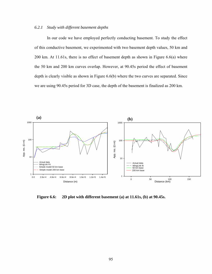
95

6.2.1 Study with different basement depths

In our code we have employed perfectly conducting basement. To study the effect

of this conductive basement, we experimented with two basement depth values, 50 km and

200 km. At 11.61s, there is no effect of basement depth as shown in Figure 6.6(a) where

the 50 km and 200 km curves overlap. However, at 90.45s period the effect of basement

depth is clearly visible as shown in Figure 6.6(b) where the two curves are separated. Since

we are using 90.45s period for 3D case, the depth of the basement is finalized as 200 km.

Figure 6.6: 2D plot with different basement (a) at 11.61s, (b) at 90.45s.

Distance (m)

0.0 2.0e+4 4.0e+4 6.0e+4 8.0e+4 1.0e+5 1.2e+5 1.4e+5

App

. res

. (Ω

-m)

1

10

100

1000

Simple model 200 km base

WingLink FitActual data

Simple model 50 km base

(a)

Distance (km)0 50 100 150

App

. res

. (Ω

-m)

1

10

100

1000

200 km base50 km baseWingLink fitActual data

(b)

96

6.2.2 Study with different block resistivities

Next, we varied the resistivity of conductive block to find the appropriate resistivity

of blocks. The responses are compared in Figure 6.7(a) and Figure 6.7(b) at 11.61s and

90.45s periods respectively. Our main emphasis is on the study of the conductive feature

near MCT. We carried out the experiment with resistivity value of this block as 5 and 8 Ω-

m keeping other parameters unchanged. It is clear that the 8 Ω-m response matches well

with the data. So, we finally used 8 Ω-m resistivity of the conductivity block for further

studies.

Figure 6.7: 2D plot with resistivity variation of conductive block (a) at 11.61s, (b) 90.45s.

Distance (km)

0 20 40 60 80 100 120 140 160 180

App.

res.

(Ω-m

)

1

10

100

1000

Data aquiredWingLink response

8 ohm-m block5 ohm-m block

(a)

1

10

100

1000

Distance (km)

0 20 40 60 80 100 120 140 160 180

App

. res

. (Ω

-m)

1

10

100

1000

5 ohm-m block

Actual dataWingLink fit

8 ohm-m block

(b)

97

6.2.3 Multi-frequency responses

Next we checked the multi-frequency response computed using present algorithm

and compared these with the field data. Two autogrids for periods 11.61s and 90.45s were

generated for this study. The responses at 11.61s using the 11.61s autogrid and the 90.45s

autogrid are compared with each other and with the field data and WinGLink response in

Figure 6.8(a). The responses for both grids matches well with each other. In Figure 6.8(b),

the 90.45s responses obtained using the 11.61s autogrid and the 90.45s autogrid are

compared and these also match well with each other and with the data values. This

experiment gives us confidence that the multi-frequency solution is not only accurate for

simple geometry models but also for complex models.

Figure 6.8: Response curves for mutifrequency using eigenmodes of 11.61s and 90.45s grid (a) at 11.61s (b) at 90.45s.

Distance (km)

App

. res

. (Ω

-m)

1

10

100

1000

0 20 40 60 80 100 120 140 160 180

Data aquiredWingLink response8 ohm-m using 11.61 grid8 ohm-m using 90.45 grid

(a)

Distance (km)

0 20 40 60 80 100 120 140 160 180

App

. res

. (Ω

-m)

1

10

100

1000

Actual dataWingLink fit 8 ohm-m using 90.45s grid8 ohm-m using 11.61 grid

(b)

98

6.2.4 Comparison with and without salient features

Since we are interested in the conductive feature near MCT and we used 90.45s

period in 3D modeling, we tested the effect of other features, such as conductive layer and

resistive block, on the response at this period only. We removed these features one by one

and compared the responses with the response of model having only the conductive block

near MCT. The response curves plotted in the Figure 6.9 reveal that the curve segment over

the conductive block is not affected by other features. Thus the 2D experiments reveal that

study of single 8 Ω-m block with basement at 200 km for time period 90.45s is good

enough for designing 3D models. The 3D nature of this conductive block can be studied as

if other features are not there.

Figure 6.9: Curves with and without the features other than conductor.

Distance (km)

0 20 40 60 80 100 120 140 160 180

App

. res

. (Ω

-m)

1

10

100

1000

Actual dataWingLink fit

Full modelonly conductive block

99

6.3 3D Experiment

From 2D experimentation it is clear that the conductive block near MCT is main

feature and its implication is presented in Figure 6.3 as many earthquakes occur near this

zone and different 3D experiments performed on this conductive block are

1) Effect of varying strike length

2) Effect of changing depth to top of the conductive block

3) Effect of varying the thickness and width of the block

6.3.1 Effect of varying the strike length

The first question that comes to mind in a 3D study is regarding the strike length of

the body. In this experiment, strike length is varied from 20 km to 100 km. The length of

the block in strike direction is taken as 20, 50, 70 and 100 km keeping other parameters

fixed. Figures 6.10(a) and 6.10(b) show the effect of strike length variation respectively for

2 km and 4 km depth to top of the block. In Figure 6.10(b), 70 km strike response lies

closest to the 2D response. From Figure 6.10(c) it is clear that the 3D response curves

approach the corresponding 2D response curve as the strike length increases.

100

Distance (m)

6.0e+4 8.0e+4 1.0e+5 1.2e+5 1.4e+5 1.6e+5

App.

res.

(Ω-m

)

50

100

150

200

250

50

100

150

200

250

2D only con block 8 ohm-m

50 km strike_20 km x70 km strike_20 km x

Distance (m)

6.0e+4 8.0e+4 1.0e+5 1.2e+5 1.4e+5 1.6e+5

App.

res.

(Ω-m

)

50

100

150

200

250

50

100

150

200

250

2D only con block 8 ohm-m

50 km strike - 20 km x70 km strike - 20 km x

6.0e+4 8.0e+4 1.0e+5 1.2e+5 1.4e+5 1.6e+510

100

1000

App

. res

. (Ω

-m)

10

100

1000

Distance (m)

20 km strike50 km strike70 km strike

2D response100 km strike

Figure 6.10: Strike variation curves for different depth to the top (a) at 2 km, (b) 4 km and (c) 6 km.

(c)

(a) (b)

101

6.3.2 Effect of changing depth to top of the conductive block

Next we experimented with different depths to the top as 2, 4 and 6 km. At 2 km

depth, curve did not follow the expected behavior outside the body as shown in Figure

6.11. In this figure the edges of the block are clearly identifiable but did not follow the 2D

response. At 4 km depth, response curve is smoother at the edges and finally it approaches

the behavior of 2D response at 70 km strike. At 6 km depth (as suggested by Tyagi (2007)

model), the response curve lies above the response curve of 4 km depth. Thus response

curve for 70 km strike and 4 km depth is the most suitable one.

Figure 6.11: Plot for depth to the top of block.

In the next experiment, the depth and strike are kept fixed to these values and only

the width of the block in other horizontal direction is varied.

Distance (m)

6.0e+4 8.0e+4 1.0e+5 1.2e+5 1.4e+5 1.6e+5

App

. res

. (Ω

-m)

50

100

150

200

250

2D response

2 km depth

6 km depth4 km depth

102

6.3.3 Effect of varying the thickness and width of the block

We observed that at 70 km strike the curve suitably lies in the best range. Then we

experimented by varying the dimension of block in orthogonal horizontal direction keeping

the depth of burial and strike fixed. The depth to the top is taken 4 km and strike is fixed at

70 km. The width of block in other horizontal direction varies as 20, 26, 40 and 50 km and

the computed responses are shown in Figure 6.12. We can observe that as width increases

the curves started flattening while bottom of the curve is approximately the same. At 50 km

width the curve seems roughly flat. Thus 20 or 26 km width may be the best for

comparison with 2D behavior.

6.4 Conclusion

From these experiments we conclude that the conductive block geometry can be

taken as 70 km strike, 20-26 km width and 4 km depth and its resistivity is 8 Ω-m. This 3D

study suggests that the conductive block is practically 2D in nature.

Distance (m)

9.0e+4 1.0e+5 1.1e+5 1.2e+5 1.3e+5

App

. res

. (Ω

-m)

50

100

150

200

250

2D only con block 8 ohm-m

70 km strike_20 km x70 km strike_26 km x70 km strike_40 km x70 km strike_50 km x

Figure 6.12: Variation in the block in other horizontal direction.

103

CHAPTER 7

SUMMARY AND CONCLUSION

The work on this thesis started with an objective of inversion of 3D magnetotelluric

data. It is well known that an efficient modeling algorithm is a prerequisite for developing a

competent inversion algorithm for data interpretation. The work presented herein is

description and discussion related with the development of an efficient 3D modeling

algorithm based on eigenmodes for magnetotelluric data.

The existing algorithms require re-run of the algorithm for each frequency. Thus, it

requires same amount of computational time for each frequency. However, using

eigenmode analysis, the multi-frequency responses are generated in negligible time once

the eigenmodes, independent of frequency, are evaluated. In this approach, the eigenmodes

depend only on the model characteristics. This efficiency is achieved by broadening the

scope of the approach given in Stuntebeck (2003). She developed the technique for limited

use of air-borne elctromagnetics for which theory is provided in her thesis. Based on that

theory we developed the algorithm for magnetotelluric data. In order to build up the sound

methodology of the algorithm, we started with 1D modeling where closed form solution of

forward problem is available. After obtaining satisfactory results in 1D case, we developed

the 2D algorithm named as MT_2D_EA and finally developed the 3D modeling algorithm

MT_3D_EA. For these algorithms, bulk of the computational time is taken for the

computation of eigenmodes. MT_2D_EA and MT_3D_EA were tested for its accuracy and

efficiency using number of 2D and 3D models, presented in the paper (Zhdanov et al.,

1997), that are numerically solved using different algorithms based on matrix solver. We

found that numerical responses obtained from the two approaches are same within

104

numerical errors. We observed that when responses for only few frequencies are computed,

the computer time consumed by MT_3D_EA is more than the matrix solver based

algorithms. However, when responses for large number of frequencies are required, a need

for MT sounding, the total computer time requirement is less in case of eigenmode based

technique than the matrix solver techniques. This is important to note here that the

computed eigenmodes in forward modeling will be used as it is in computation of

sensitivity matrix while developing the inversion software for 3D MT data.

The algorithm is employed to generate 3D models for the field data, acquired by

Israil et al. (2008) in Garhwal Himalaya. On the basis of 2D interpretation of this data set,

Israil et al. (2008) proposed a 2D electrical model of the region. The key feature of this 2D

model is a conductor near MCT. We studied the 3D nature of this conductor and found that

the 2D approximation of the conductor was justified.

The present algorithm is based on solving the secondary field EM eigenvalue

problem using Finite Difference Method (FDM). The electric field values for any source

are evaluated as superposition of the eigenvectors. The staggered grid, as proposed by Yee

(1966), is used for accurate EM field computations. The FDM is used to transformed the

EM eigenproblem to a symmetric matrix eigenproblem. It is found that one third of the

eigenvalues of the 13-diagonal symmetric matrix becomes zero. As per concept of physics

the zero eigenvalues and corresponding eigenvectors are not part of any physical system

and we termed these as spurious eigenmodes. These eigenvalues are taken out of the study.

by eliminating, using current divergence relation, the ez components from the system of

equations. Now the system of equations deals only with the horizontal components ex and

ey. This step reduces size of the resulting matrix to two third of the symmetric matrix.

105

However, the outcome of this reduction converts the symmetric matrix to non-symmetric.

The eigenvalues and eigenvectors of the reduced non-symmetric matrix are computed. The

electric field is continued analytically into the air through integral boundary condition. This

step results in making nonzero all elements of the submatrix block corresponding to air-

earth interface nodes.

Lanczos/Arnoldi method is used for evaluating the eigenmodes of symmetric/non-

symmetric matrix. From the eigenmode formulation it is clear that, during superposition,

only a subset of the smallest eigenvalues contributes significantly to the synthesis of field

values. To get this subset of eigenmodes, Implicitly Restarted Lanczos/Arnoldi Method

(IRLM/IRAM) is used in invert mode where product of inverse of the matrix with a vector

is used. BiCGStab (Bi-Conjugate Gradient Stabilized) with preconditioner ILU(0) is used

to efficiently obtain this product.. During the iterations of Arnoldi method, the eigenvectors

loose their orthogonality. To reinstate orthogonality, the Arnoldi steps are applied twice.

Only the non-zero elements of the coefficient matrix are stored to reduce the memory

requirement. IRAM provides the eigenvalues and reduced eigenvectors, containing only the

horizontal components ex and ey. For each eigenvector, the ez components are then obtained

by using the current divergence relation. These full eigenvectors are made sigma-

orthogonal. The eigenvalues and sigma-orthogonalized eigenvectors are next used to obtain

the secondary electric field values. The primary electric field is already computed using

layered earth model response. The total electric field values are obtained from primary and

secondary electric field values. The total electric field values are used to derive the

magnetic field. The electric field and magnetic field values are then used to compute

impedance, apparent resistivity and phase values.

106

7.1 Conclusion

The algorithms, MT_2D_EA and MT_3D_EA developed in this thesis, are efficient

and reliable softwares respectively for 2D and 3D magnetotelluric modeling. The

algorithms have been rigorously and comprehensively tested within the limited time frame

of this study and under the severe constraint on size of the 3D problem imposed by

capacity of the available computer facility. This limitation, however, led us to perform

detailed study of the effect of coarse grid on the EM response. Numerous experiments were

performed to test the consistency and accuracy of the algorithms. These tests justified a

qualified faith in the algorithms MT_2D_EA and MT_3D_EA. The results of various

design exercises and comparison of the computed responses of different models with

published ones, lead us to following conclusions

• The algorithm is able to model a complex structure.

• The eigenmode computations consume bulk of the computer resources and

time. However, these are to be performed only once, even when responses for

numerous frequencies are to be computed.

• Given the eigenmodes, the algorithm is capable of generating muti-frequency

responses at a marginal cost.

• For conductive target use of only 5% eigenmodes is sufficient while for

resistive target one must use 20% eigenmodes. So, this algorithm, in its present

form, works better for conductive targets.

• In Garhwal Himalaya, the 3D geometry of the conductive block, buried under

the Roorkee-Gangotri profile near MCT, can be taken as 70 km strike, 20-26

km width and 4 km depth and its resistivity is estimated as 8 Ω-m. However, the

107

detailed 3D study suggests that the conductive block can be approximated as a

2D one.

7.2 Limitations of the Algorithm

The limitations of the algorithm identified during testing are as follows.

• Presently, the manually generated grid is used in the algorithm.

• The algorithm takes major time in eigenmode computation.

• At the bottom of the modeling domain, perfectly conducting boundary condition

is employed in the algorithm. This constraint forces one to take bottom at

sufficient distance so that the tangential electric field will be zero at the domain

boundary.

• Presently the algorithm can be used only for the plane wave source.

• The isotropic medium can be modeled using the algorithm.

7.3 Suggestions for Future Work

The present thesis has turned out to be an exploratory effort during which the

computer programs MT_2D_EA and MT_3D_EA have been developed with an aim to

enable quantitative interpretation of 3D MT data. The limitations listed above suggest that

there exists a significant scope for further development. The limitations mentioned can be

minimized by taking following steps.

• Implementation of auto grid generator which employs the skin depth criterion.

• Significant improvement can be made in the eigenmode evaluation, especially

by using customized preconditioner in BiCGSTAB subprogram.

108

• Implementation of integral boundary condition at the bottom boundary of the

domain.

• The algorithm can be modified for the computation of responses in case of

controlled source EM methods simply by replacing the present primary field

response computation subprogram with one corresponding to the given EM

source.

• Inclusion of anisotropy.

• Adaptation of the MT_3D_EA code for parallel programming.

Finally, it may be stressed that after the code is adapted for parallel programming,

the use of clusters of computers and supercomputers will significantly reduce the

computational time and make it possible to undertake development of 3D MT data

inversion algorithm.

109

APPENDIX A1

INTERGRAL BOUNDARY CONDITION

The electric field is not constant at the air earth interface. It is decaying in the air

also. This effect is taken into account by applying, at the air-earth interface, the integral

boundary condition which models the continuation of electric field up to large distances in

air. The integral boundary condition is described below.

A1.1 Integral Boundary Condition at the Air-Earth Interface

We are taking z +ve in downward direction. So, in the air, z is negative (z<0). In the

air ( 0=σ ) Maxwell’s vector equations are reduced to

BE &−=×∇ , (A1.1)

0=×∇ B . (A1.2)

Taking divergence of equation (A1.1) we get

0=⋅∇ B& . (A1.3)

Further, equation (A1.2) permits the substitution

φ∇=B . (A1.4)

Equations (A1.3) and (A1.4) together yield

02 =∇ φ . (A1.5)

The equation (A1.5) can be recast as

2

2

2

2

2

2

)(yxz

z∂∂

−∂∂

−=∂∂

=′′ φφφφ , (A1.6)

Assuming exponential z-dependence of ),,( zyxφ , it can be expressed as

110

)exp(),(),,( zyxuzyx χφ = . (A1.7)

Substituting this relation into equation (A1.6) we get,

),(),( 22

2

2

2

yxuyxuyx

χ=⎟⎟⎠

⎞⎜⎜⎝

⎛∂∂

+∂∂

− (A1.8)

Let the plane at air-earth interface in discretized into nxy cells, the LHS of equation (A1.8)

after use of finite differences, gets transformed to a matrix F which is symmetric and

positive semi-definite. The discretized version of equation (A1.8) can be written as

jjjF uu 2χ= , j = 1,nxy. (A1.9)

Here, uj is the eigenvector corresponding to the eigenvalue 2jχ of the coefficient matrix.

Any vector can be expressed as linear superposition of orthogonal eigenvectors as

∑=j

jjc uu . (A1.10)

The coefficient cj’s can be evaluated using the known value of zb& at air-earth interface

(z=0) which can be described as

),()0( 2 yxuz jz χφ ==′′−=b& , (A1.11)

and

)0(1

2=⋅= zz

j

bu &χ

. (A1.12)

Using equations (A1.12) and (A1.10), the coefficient of superposition can be evaluated as

jzj

j zc ub ⋅=⋅= )0(1

2&

χ. (A1.13)

Finally, ),,( zyxφ can recast using (A1.7), (A1.10) and (A1.13) as

)exp()0(1

),,(1

2zuuzzyx j

Tjj

n

j j

xy

χχ

φ ==∑=

zb& . (A1.14)

111

This integral boundary condition relation (A1.14) provides the matrix coefficients

due to electric field continuation in the air. Here, nxy is the number of horizontal electric

field components at air-earth interface.

113

APPENDIX A2

MATRIX COEFFICIENTS AND SIGMA

ORTHONORMALIZATION The eigenmode algorithm, using FDM, is described in Chapter 3. The components

of the electric field are described here along with the average volume and the average

conductivity definitions. The 13 non-zero coefficient values for all the three electric field

components are given. The eigenvectors are not simple orthogonal, rather these follow

sigma orthogonality and its implementation in terms of a constant factor multiplication to

the simply orthogonal eigenvector is discussed.

A2.1 Matrix Coefficients

The average conductivities xσ , yσ and zσ associated with the points of cell (i, j, k),

where ex, ey and ez components are evaluated, are given by the following relations,

⎥⎦

⎤⎢⎣

⎡−−+−−−−+

−−+=

)1,,()1()()1,1,()1()1(),1,()()1(),,()()(

),,(4)(),,(

kjikcjbkjikcjbkjikcjbkjikcjb

kjiViakji

xx σσ

σσσ ,

⎥⎦

⎤⎢⎣

⎡−−+−−−−+

−−+=

)1,,()1()()1,,1()1()1(),,1()()1(),,()()(

),,(4)(),,(

kjikciakjikciakjikciakjikcia

kjiVjbkji

yy σσ

σσσ ,

⎥⎦

⎤⎢⎣

⎡−−+−−−−+

−−+=

),1,()1()(),1,1()1()1(),,1()()1(),,()()(

),,(4)(),,(

kjijbiakjijbiakjijbiakjijbia

kjiVkckji

zz σσ

σσσ

------ (A2.1)

Here, the volumes Vx, Vy and Vz are

)()()(),,( kchjbhiakjiVx = ,

)()()(),,( kchjbiahkjiVy = ,

114

)()()(),,( kcjbhiahkjiVz = . (A2.2)

The matrix symmetry is conserved by the transformations

),,(),,(),,(),,( 0 kjiekjikjiVkjie xxxx σµ= ,

),,(),,(),,(),,( 0 kjiekjikjiVkjie yyyy σµ= ,

),,(),,(),,(),,( 0 kjiekjikjiVkjie zzzz σµ= . (A2.3)

This transformation is valid only for points with non-zero ),,( kjixσ , ),,( kjiyσ and

),,( kjizσ . Using the abbreviations

),,(),,(1),,( 0 kjikjiVkjid xxx σµ= ,

),,(),,(1),,( 0 kjikjiVkjid yyy σµ= ,

),,(),,(1),,( 0 kjikjiVkjid zzz σµ= , (A2.4)

the system equations for the transformed electric components become

⎪⎪⎪⎪⎪⎪⎪⎪⎪

⎭

⎪⎪⎪⎪⎪⎪⎪⎪⎪

⎬

⎫

⎪⎪⎪⎪⎪⎪⎪⎪⎪

⎩

⎪⎪⎪⎪⎪⎪⎪⎪⎪

⎨

⎧

+++−−+−+−−−+

+++−

−+−+−−−+

++−−−−

−

++−−−−

−

⎥⎦

⎤⎢⎣

⎡−

++−

+

⋅=

),,1(),,1()(),,(),,()(

),,1(),,1()(),,(),,()(

),1,1(),1,1()(),1,(),1,()(

)1,,()1,,()(

)()(

),1,(),1,()(

)()(),1,(),1,()1()()(

),,(),,()1()()(

)()()(

)1()()(

)()()(

),,(),,(

kjiekjidjbhkjiekjidjbh

kjiekjidkchkjiekjidkchkjiekjidkchkjiekjidkch

kjiekjidkc

jbhia

kjiekjidjb

kchiakjiekjidjb

kchia

kjiekjidkc

jbhiakc

jbhiajb

kchiajb

kchia

kjidkjie

zzzz

yyyy

yyyy

xx

xxxx

xx

xx

1)kj,1,(ie1)kj,1,(ibh(j)d1)kj,(i,e1)kj,(i,bh(j)d

1)kj,(i,e1)kj,(i,d1)c(k

a(i)bh(j)

zzzz

xx

λ

------- (A2.5)

115

⎪⎪⎪⎪⎪⎪⎪⎪⎪

⎭

⎪⎪⎪⎪⎪⎪⎪⎪⎪

⎬

⎫

⎪⎪⎪⎪⎪⎪⎪⎪⎪

⎩

⎪⎪⎪⎪⎪⎪⎪⎪⎪

⎨

⎧

+++−+−+−−−−+

+++−−+−+−−−+

++−−−−

−

++−−−−

−

⎥⎦

⎤⎢⎣

⎡−

++−

+

⋅=

),1,(),1,()(),,(),,()(),1,1(),1,1()(),,1(),,1()(

),1,(),1,()(),,(),,()(

),,1(),,1()(

)()(),,1(),,1()1(

)()(

)1,,()1,,()(

)()(

),,(),,()1(

)()()(

)()()1()()(

)()()(

),,(),,(

kjiekjidkchkjiekjidkchkjiekjidkchkjiekjidkch

kjiekjidiahkjiekjidiah

kjiekjidia

kchjbkjiekjidia

kchjb

kjiekjidkc

jbiah

kjiekjidia

kchjbia

kchjbkc

jbiahkc

jbiah

kjidkjie

zzxx

xxxx

zzzz

yyyy

yy

yy

yy 1)k1,j(i,e1)k1,j(i,ah(i)d1)kj,(i,e1)kj,(i,ah(i)d

1)kj,(i,e1)kj,(i,d1)c(k

ah(i)b(j)

zzzz

yy

λ

------ (A2.6)

⎪⎪⎪⎪⎪⎪⎪⎪⎪

⎭

⎪⎪⎪⎪⎪⎪⎪⎪⎪

⎬

⎫

⎪⎪⎪⎪⎪⎪⎪⎪⎪

⎩

⎪⎪⎪⎪⎪⎪⎪⎪⎪

⎨

⎧

+++−

+−+−−−−++++−

+−+−−−−+

++−−−−

−

++−−−−

−

⎥⎦

⎤⎢⎣

⎡+

−++

−

⋅=

)1,,()1,,()(),,(),,()(

)1,1,()1,1,()(),1,(),1,()()1,,()1,,()(),,(),,()(

)1,,1()1,,1()(),,1(),,1()(

),1,(),1,()(

)()(),1,(),1,()1()()(

),,1(),,1()(

)()(),,1(),,1()1(

)()(

),,(),,()(

)()()1()()(

)()()(

)1()()(

),,(),,(

kjiekjidiahkjiekjidiahkjiekjidiahkjiekjidiah

kjiekjidjbhkjiekjidjbhkjiekjidjbhkjiekjidjbh

kjiekjidjb

kciahkjiekjidjb

kciah

kjiekjidia

kcjbhkjiekjidia

kcjbh

kjiekjidjb

kciahjb

kciahia

kcjbhia

kcjbh

kjidkjie

yyyy

yyyy

xxxx

xxxx

zzzz

zzzz

zz

zzλ

------ (A2.7)

116

In the above equations the bold terms do not contribute in the first layer, bounded by air-

earth interface, and these are replaced with field continuation coefficients given by

equation (A1.14) of Appendix A1. The complete system of equations can be represented as

eeA λ= . (A2.8)

Here, A matrix contains elements due to field continuation as well as due to FD

approximation of equations (A2.5), (A2.6) and (A2.7).

The ez components are replaced with the horizontal components using the current

divergence relation (equation 3.19). This leads to a non-symmetric matrix as shown in

Figure 3.5. Now the reduced system of equation can be written as

eeAR(( λ= , (A2.9)

where, AR denotes the reduced matrix and e( denotes the reduced eigenvector

having only horizontal components. These reduced eigenvectors, e( , are orthogonal. The full

eigenvectors, ē, are now reconstructed from these reduced eigenvectors, e( , using the

divergence relation again. These full eigenvectors are sigma-orthonormalized as discussed

below.

A2.2 Sigma Orthogonality of Eigenvectors

The full eigenvectors, ē, are transformed, using equation (A2.3), into eigenvectors,

e. These transformed eigenvectors must be σ-orthonormal as stated in Chapter 2. The σ-

orthonormality relation as described in equation (2.24) is

∫ = nmrdr δσ 3ˆˆ)( mnee . (A2.10)

Let the final σ-orthogonal eigenvectors, ne , with weighted norm nη be defined as

)()(ˆ rr n nn ee η= . (A2.11)

117

The orthogonality relation (A2.10) in discrete form can be written as

nm

N

rrVrrr

A

δσ =∑=

)()(ˆ)(ˆ)(1

mn ee . (A2.12)

The norm factor nη is obtained by applying weighted normalization as follows

1)()()()()(ˆ)(1

22

1

2 ==∑∑==

rVrrrVrrAA N

rnn

N

rn ee ησσ ,

2

1

2 /1)()()( n

N

rn rVrr

A

ησ =∑=

e . (A2.13)

Using the relation (A2.3), the eigenvectors ne transformed into eigenvectors ne , the norm

factor simplifies to

0

1

2

0

1

2

0

)()(11 µ

µ

µ

η ===

∑∑==

AA N

rn

N

rn

n

rr ee, (A2.15)

assuming 1=ne .

Thus, the eigenvectors ne with weighted norm, which are needed for eigenmode synthesis,

are determined directly from the orthonormal eigenvectors ne by

).()()()(ˆ 0 rrdrr nnn eee µη == (A2.16)

119

APPENDIX A3

ALGORITHM PARAMETERS AND SUBPROGRAMS

The algorithm description is given in Chapter 4. The input data and other

parameters are controlled by several counters. The details of these counters along with their

default values and descriptions are presented in Table A3.1. The grid control parameters

are given in Table A3.2. In Table A3.3, the list of subprograms is presented along with

their purposes.

Table A3.1: Description of control parameters.

Parameter Controls Value Description

irx Grid generation in x-direction

0 1

Manual grid Logarithmic grid

iry Grid generation in y-direction

0 1

Manual grid Logarithmic grid

irz Grid generation in z-direction

0 1

Manual grid Logarithmic grid

irt No of time periods in decades

0 1

Manual time period Logarithmic time

period

irun Generation of eigenmodes

0 1

Generate eigenmodes

Reused eigenmodes

mode_type Response computation

corresponding to 2D

0 1

corresponding to 2D TE mode

Corresponding to 2D TM mode

preconditioner Which preconditioner

0 1 2

No preconditioner 9-diag

precconditioner Block

preconditioner

Table A3.1 continues……

120

restart Eigenmode computation

0 1

All eigenmodes Desired Eigenmodes

Table A3.2: Grid parameters description.

Parameter Description

nx Number of cells in x-direction

ny Number of cells in y-direction

nz Number of cells in z-direction

ne Number of ex + ey components

nef Total number of unknowns (ex + ey + ez components)

np

Number of anomalous prisms

nt

Total number of time periods

qx (irx.eq.1) Logarithmic grid control parameter in x-direction

qx (irx.eq.1) Logarithmic grid control parameter in y-

direction

qx (irx.eq.1) Logarithmic grid control parameter in z-direction

tz (irt.eq.1) Logarithmic time distribution control

parameter

rho0

Half space resistivity

rho1,…np

Anomalous resistivity

ixa

Starting cell number of anomalous prism in x-direction

ixb

Ending cell number of anomalous prism in

x-direction

Table A3.2 continues…..

……Table A3.1 continued

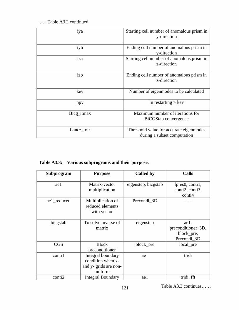
121

iya

Starting cell number of anomalous prism in y-direction

iyb

Ending cell number of anomalous prism in

y-direction iza

Starting cell number of anomalous prism in

z-direction

izb

Ending cell number of anomalous prism in z-direction

kev

Number of eigenmodes to be calculated

npv

In restarting > kev

Bicg_itmax

Maximum number of iterations for BiCGStab convergence

Lancz_tolr

Threshold value for accurate eigenmodes

during a subset computation

Table A3.3: Various subprograms and their purpose.

Subprogram

Purpose Called by Calls

ae1

Matrix-vector multiplication

eigenstep, bicgstab fpres0, conti1, conti2, conti3,

conti4 ae1_reduced

Multiplication of reduced elements

with vector

Precondi_3D ------

bicgstab

To solve inverse of matrix

eigenstep ae1, preconditioner_3D,

block_pre, Precondi_3D

CGS

Block preconditioner

block_pre local_pre

conti1

Integral boundary condition when x-

and y- grids are non-uniform

ae1 tridi

conti2 Integral Boundary ae1 tridi, fft

……Table A3.2 continued

Table A3.3 continues……

122

condition when x-is non-uniform and y-

is uniform

conti3

Integral boundary condition when x-is

uniform and Y-is non-uniform

ae1 tridi, fft

conti4

Integral boundary condition when both

x- and y- are uniform

ae1 fft

dlahqr

Eigenmode computation of 3D

eigenmode_3d ------

dnapps

Updation of a subset of eigenmodes

eigenmode_3d Adepted/taken from ARPACK

eigenmode_1D Eigenmode computation for 1D

layered structure

Main Tridi

eigenmode_3D Computing 3D eigenmodes

Main dnapps, eigenstep, dlahqr, gramsmdt,

get_ez eigenstep Generation of

Heisenberg matrix and new starting

vector

eigenmode_3d ae1, bicgstab

extremal

Limits of eigenvalues computation

Main ------

fft

Forward/Inverse Fourier transform

conit2, conti3, conti4

------

fpres0

Surface field computation

ae1 printr

get_ez

Solving ez components of

eigenvectors from reduced

eigenmode_3d ------

……Table A3.3 continued

Table A3.3 continues……

123

eigenvectors

gramsmdt

Orthogonalization of new eigenvector

with previous eigenvectors

eigenmode_3d ------

grid

Generation of logarithmic grid

input ------

init

Initialization of starting vector

Main ------

input

Read input and control parameters

Main grid, sigma0, sigma1, sigma2

local_pre

Local (block wise) CGS ------

method

Identification of uniform or non-

uniform grid

Main ------

output_1d

Primary field computation

Main ------

output_3d

Total E-field, Impedance,

Apparent resistivity and Phase

computation for 3D

Main ------

Pre_1

To multiply continuation element for

preconditioning

block_pre conti1, conti2, conti3, conti4

Pre_2 Multiplication of Reduced

components for preconditioning

block_pre ------

Pre_3

Multiplying each block with the vector element

CGS ------

Pre_4

Preconditioner element

Pre_1 ------

……Table A3.3 continued

Table A3.3 continues……

124

Precondi_3D

First 9-diagonal preconditioner the reduces element

iteratively

bicgstab Preconditioner_3D, ae1_reeduced

Preconditioner_3D

9-diag preconditioner

bicgstab, Pre_3 ------

printi

Print 3D integer array

sigma0 ------

printr Print resistivity 3D array

sigma1, sigma2 ------

sigma0 Defining half space resistivity to all

nodes

input printr

sigma1

Defining anomalous nodal resistivity

values

input printr

sigma2

Average resistivity computation

input printr

tridi

Eigenmodes computation of

Symmetric tridiagonal matrix

conti1, conti2, conti3,

eigenmode_1d

------

weight

Coefficient computation for ex,

ey and ez components

Main ------

weight_ez

Coefficient corresponding to

replacing ez into ex and ey components

Main ------

……Table A3.3 continued

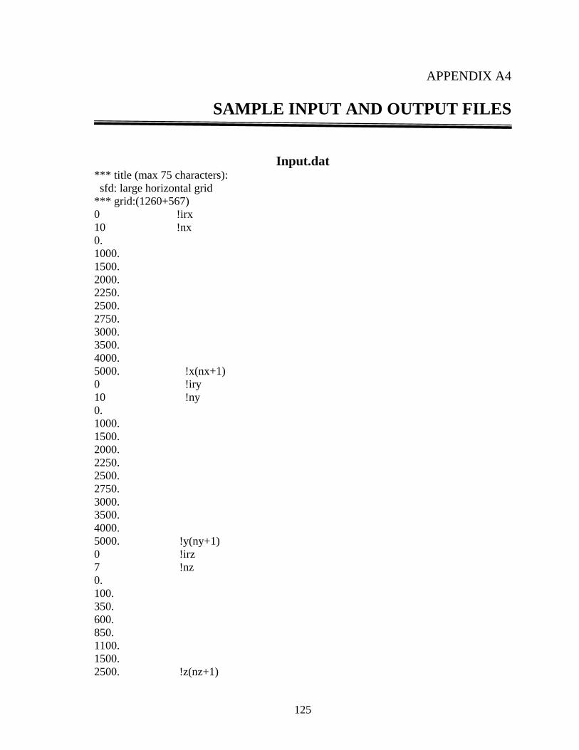
125

APPENDIX A4

SAMPLE INPUT AND OUTPUT FILES

Input.dat

*** title (max 75 characters): sfd: large horizontal grid *** grid:(1260+567) 0 !irx 10 !nx 0. 1000. 1500. 2000. 2250. 2500. 2750. 3000. 3500. 4000. 5000. !x(nx+1) 0 !iry 10 !ny 0. 1000. 1500. 2000. 2250. 2500. 2750. 3000. 3500. 4000. 5000. !y(ny+1) 0 !irz 7 !nz 0. 100. 350. 600. 850. 1100. 1500. 2500. !z(nz+1)

126

*** resistivity: 1.0 !rho00 (half space resistivity) 1 !np (number of anamalous prisms) 0.1 !rho01 (resistivity of prisms) 005 006 005 006 002 003 !ixa,ixb,iya,iyb,iza,izb 9 !iws0 0 !iws1 0 !iws2 *** time lags: 0 !irt 1 !nt 1.0 !it *** error bounds 1.0E-16 !lancz_tolr 14000 !bicg_itmax 1.0E-06 !bicg_tol 1.0E-16 !bicg_stol *** parameters controlling the Lanczos process: 1 !restart (0-> computing all eigenvalues, 1-> computing desired eigenvalues) 0 !preconditioner (0-> no pre, 1-> 9 diag pre, 2-> block pre) 1300 !mmax 1260,0 !kev,npv 0 !irun (0-> regenerate, 1-> reused eigenvectors) 0 !mode_type (1-> corresponds to 2D TE, 0-> 2D TM)

127

Output_main.dat *** title (max 75 characters): sfd: large horizontal grid *** grid:(1260+567) 0 !irx 10 !nx 0. 1000. 1500. 2000. 2250. 2500. 2750. 3000. 3500. 4000. 5000. !x(nx+1) 0 !iry 10 !ny 0. 1000. 1500. 2000. 2250. 2500. 2750. 3000. 3500. 4000. 5000. !y(ny+1) 0 !irz 7 !nz 0. 100. 350. 600. 850. 1100. 1500. 2500. !z(nz+1) *** resistivity: 1.0 !rho00 (half space resistivity) 1 !np (number of anamalous prisms) 0.1 !rho01 (resistivity of prisms) 005 006 005 006 002 003 !ixa,ixb,iya,iyb,iza,izb

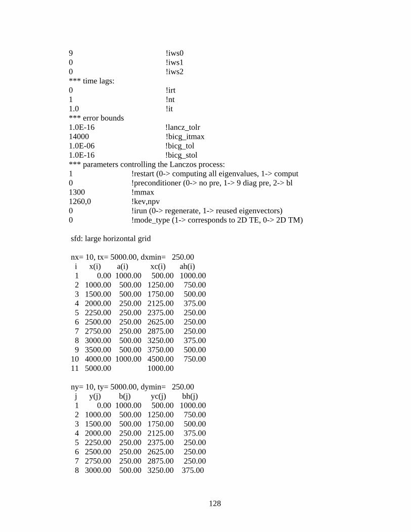
128

9 !iws0 0 !iws1 0 !iws2 *** time lags: 0 !irt 1 !nt 1.0 !it *** error bounds 1.0E-16 !lancz_tolr 14000 !bicg_itmax 1.0E-06 !bicg_tol 1.0E-16 !bicg_stol *** parameters controlling the Lanczos process: 1 !restart (0-> computing all eigenvalues, 1-> comput 0 !preconditioner (0-> no pre, 1-> 9 diag pre, 2-> bl 1300 !mmax 1260,0 !kev,npv 0 !irun (0-> regenerate, 1-> reused eigenvectors) 0 !mode_type (1-> corresponds to 2D TE, 0-> 2D TM) sfd: large horizontal grid nx= 10, tx= 5000.00, dxmin= 250.00 i x(i) a(i) xc(i) ah(i) 1 0.00 1000.00 500.00 1000.00 2 1000.00 500.00 1250.00 750.00 3 1500.00 500.00 1750.00 500.00 4 2000.00 250.00 2125.00 375.00 5 2250.00 250.00 2375.00 250.00 6 2500.00 250.00 2625.00 250.00 7 2750.00 250.00 2875.00 250.00 8 3000.00 500.00 3250.00 375.00 9 3500.00 500.00 3750.00 500.00 10 4000.00 1000.00 4500.00 750.00 11 5000.00 1000.00 ny= 10, ty= 5000.00, dymin= 250.00 j y(j) b(j) yc(j) bh(j) 1 0.00 1000.00 500.00 1000.00 2 1000.00 500.00 1250.00 750.00 3 1500.00 500.00 1750.00 500.00 4 2000.00 250.00 2125.00 375.00 5 2250.00 250.00 2375.00 250.00 6 2500.00 250.00 2625.00 250.00 7 2750.00 250.00 2875.00 250.00 8 3000.00 500.00 3250.00 375.00

129

9 3500.00 500.00 3750.00 500.00 10 4000.00 1000.00 4500.00 750.00 11 5000.00 1000.00 nz= 7, tz= 2500.00, dzmin= 100.00 k z(k) c(k) zc(k) ch(k) 1 0.00 100.00 50.00 100.00 2 100.00 250.00 225.00 175.00 3 350.00 250.00 475.00 250.00 4 600.00 250.00 725.00 250.00 5 850.00 250.00 975.00 250.00 6 1100.00 400.00 1300.00 325.00 7 1500.00 1000.00 2000.00 700.00 8 2500.00 1000.00 dhmin= 250.00, dmin= 100.00 background resistivity rho0= 1.0000E+00 Ohm*m relative position of prisms: --------------------------- i ixa ixb iya iyb iza izb 1 5 6 5 6 2 3 resistivity and absolute position of prisms: ------------------------------------------- i rho[Ohm*m] xa[m] xb[m] ya[m] yb[m] za[m] zb[m] 1 0.10000 2250.0 2750.0 2250.0 2750.0 100.0 600.0 iws0= 7: symbolic display of resistivity in the uppermost 7 levels iws1=0: no display of resistivity iws2=0: no display of averaged conductivity smin= 1.000E+00 S/m, smax= 1.000E+01 S/m is --- is - level 1: 1 2 3 4 5 6 7 8 9 10 10 0 0 0 0 0 0 0 0 0 0 9 0 0 0 0 0 0 0 0 0 0 8 0 0 0 0 0 0 0 0 0 0 7 0 0 0 0 0 0 0 0 0 0 6 0 0 0 0 0 0 0 0 0 0 5 0 0 0 0 0 0 0 0 0 0 4 0 0 0 0 0 0 0 0 0 0 3 0 0 0 0 0 0 0 0 0 0 2 0 0 0 0 0 0 0 0 0 0 1 0 0 0 0 0 0 0 0 0 0

130

is - level 2: 1 2 3 4 5 6 7 8 9 10 10 0 0 0 0 0 0 0 0 0 0 9 0 0 0 0 0 0 0 0 0 0 8 0 0 0 0 0 0 0 0 0 0 7 0 0 0 0 0 0 0 0 0 0 6 0 0 0 0 1 1 0 0 0 0 5 0 0 0 0 1 1 0 0 0 0 4 0 0 0 0 0 0 0 0 0 0 3 0 0 0 0 0 0 0 0 0 0 2 0 0 0 0 0 0 0 0 0 0 1 0 0 0 0 0 0 0 0 0 0 is - level 3: 1 2 3 4 5 6 7 8 9 10 10 0 0 0 0 0 0 0 0 0 0 9 0 0 0 0 0 0 0 0 0 0 8 0 0 0 0 0 0 0 0 0 0 7 0 0 0 0 0 0 0 0 0 0 6 0 0 0 0 1 1 0 0 0 0 5 0 0 0 0 1 1 0 0 0 0 4 0 0 0 0 0 0 0 0 0 0 3 0 0 0 0 0 0 0 0 0 0 2 0 0 0 0 0 0 0 0 0 0 1 0 0 0 0 0 0 0 0 0 0 is - level 4: 1 2 3 4 5 6 7 8 9 10 10 0 0 0 0 0 0 0 0 0 0 9 0 0 0 0 0 0 0 0 0 0 8 0 0 0 0 0 0 0 0 0 0 7 0 0 0 0 0 0 0 0 0 0 6 0 0 0 0 0 0 0 0 0 0 5 0 0 0 0 0 0 0 0 0 0 4 0 0 0 0 0 0 0 0 0 0 3 0 0 0 0 0 0 0 0 0 0 2 0 0 0 0 0 0 0 0 0 0 1 0 0 0 0 0 0 0 0 0 0 is - level 5: 1 2 3 4 5 6 7 8 9 10 10 0 0 0 0 0 0 0 0 0 0 9 0 0 0 0 0 0 0 0 0 0 8 0 0 0 0 0 0 0 0 0 0 7 0 0 0 0 0 0 0 0 0 0

131

6 0 0 0 0 0 0 0 0 0 0 5 0 0 0 0 0 0 0 0 0 0 4 0 0 0 0 0 0 0 0 0 0 3 0 0 0 0 0 0 0 0 0 0 2 0 0 0 0 0 0 0 0 0 0 1 0 0 0 0 0 0 0 0 0 0 is - level 6: 1 2 3 4 5 6 7 8 9 10 10 0 0 0 0 0 0 0 0 0 0 9 0 0 0 0 0 0 0 0 0 0 8 0 0 0 0 0 0 0 0 0 0 7 0 0 0 0 0 0 0 0 0 0 6 0 0 0 0 0 0 0 0 0 0 5 0 0 0 0 0 0 0 0 0 0 4 0 0 0 0 0 0 0 0 0 0 3 0 0 0 0 0 0 0 0 0 0 2 0 0 0 0 0 0 0 0 0 0 1 0 0 0 0 0 0 0 0 0 0 is - level 7: 1 2 3 4 5 6 7 8 9 10 10 0 0 0 0 0 0 0 0 0 0 9 0 0 0 0 0 0 0 0 0 0 8 0 0 0 0 0 0 0 0 0 0 7 0 0 0 0 0 0 0 0 0 0 6 0 0 0 0 0 0 0 0 0 0 5 0 0 0 0 0 0 0 0 0 0 4 0 0 0 0 0 0 0 0 0 0 3 0 0 0 0 0 0 0 0 0 0 2 0 0 0 0 0 0 0 0 0 0 1 0 0 0 0 0 0 0 0 0 0 explanation: 0: rho= 1.00 Ohm*m 1: rho= 0.10 Ohm*m time lags and extremal diffusion lengths: ---------------------------------------- it t[s] d_min[m] d_max[m] d_bgr[m] 1 1.000E+00 2.821E+02 8.921E+02 8.921E+02 bgr=background convergence check after mstep=1260 iterations alphmin= 7.8540E-03, alphmax= 1.6000E+02 meth=1: no-fft grid in x- and y-direction 1D eigenvalues: no., value 1 6.95E+01 2 4.33E+01 3 2.75E+01 4 1.34E+01 5 5.13E+00 6 1.15E+00

132

Final eigenvalues of 3D problem 8.62E-01 8.62E-01 9.01E-01 1.25E+00 1.74E+00 1.74E+00 1.87E+00 1.87E+00 2.19E+00 2.19E+00 2.60E+00 3.09E+00 3.12E+00 3.13E+00 3.24E+00 3.24E+00 3.25E+00 3.35E+00 3.35E+00 3.65E+00 3.65E+00 3.82E+00 3.97E+00 3.97E+00 4.03E+00 4.03E+00 4.46E+00 4.46E+00 4.52E+00 4.54E+00 4.87E+00 4.87E+00 4.96E+00 5.30E+00 5.39E+00 5.48E+00 5.48E+00 5.49E+00 5.60E+00 5.79E+00 5.88E+00 5.94E+00 5.94E+00 5.94E+00 6.11E+00 6.11E+00 6.26E+00 6.26E+00 6.37E+00 6.38E+00 6.52E+00 6.52E+00 6.56E+00 6.83E+00 6.83E+00 6.96E+00 7.15E+00 7.15E+00 7.34E+00 7.64E+00 7.76E+00 7.76E+00 7.93E+00 7.93E+00 8.02E+00 8.19E+00 8.19E+00 8.36E+00 8.40E+00 8.45E+00 8.45E+00 8.69E+00 8.74E+00 8.74E+00 8.74E+00 8.78E+00 8.94E+00 8.99E+00 8.99E+00 9.06E+00 9.10E+00 9.15E+00 9.15E+00 9.22E+00 9.22E+00 9.40E+00 9.40E+00 9.80E+00 9.83E+00 9.83E+00 9.98E+00 1.00E+01 1.00E+01 1.01E+01 1.03E+01 1.03E+01 1.04E+01 1.05E+01 1.05E+01 1.06E+01 1.06E+01 1.06E+01 1.06E+01 1.08E+01 1.08E+01 1.08E+01 1.09E+01 1.09E+01 1.09E+01 1.10E+01 1.11E+01 1.11E+01 1.11E+01 1.11E+01 1.11E+01 1.12E+01 1.12E+01 1.13E+01 1.14E+01 1.14E+01 1.14E+01 1.15E+01 1.15E+01 1.15E+01 1.16E+01 1.16E+01 1.17E+01 1.17E+01 1.18E+01 1.18E+01 1.21E+01 1.21E+01 1.21E+01 1.22E+01 1.22E+01 1.23E+01 1.24E+01 1.24E+01 1.24E+01 1.25E+01 1.28E+01 1.28E+01 1.28E+01 1.29E+01 1.29E+01 1.30E+01 1.30E+01 1.30E+01 1.31E+01 1.31E+01 1.32E+01 1.32E+01 1.34E+01 1.36E+01 1.36E+01 1.37E+01 1.37E+01 1.37E+01 1.37E+01 1.38E+01 1.41E+01 1.41E+01 1.41E+01 1.41E+01 1.42E+01 1.43E+01 1.44E+01 1.44E+01 1.45E+01 1.46E+01 1.47E+01 1.47E+01 1.49E+01 1.49E+01 1.50E+01 1.53E+01 1.53E+01 1.54E+01 1.54E+01 1.54E+01 1.54E+01 1.54E+01 1.55E+01 1.55E+01 1.55E+01 1.56E+01 1.58E+01 1.59E+01 1.60E+01 1.60E+01 1.60E+01 1.60E+01 1.61E+01 1.65E+01 1.66E+01 1.66E+01 1.67E+01 1.67E+01 1.68E+01 1.70E+01 1.70E+01 1.73E+01 1.73E+01 1.74E+01 1.76E+01 1.76E+01 1.76E+01 1.78E+01 1.78E+01 1.78E+01 1.79E+01 1.80E+01 1.81E+01 1.81E+01 1.81E+01 1.83E+01 1.83E+01 1.83E+01 1.83E+01 1.83E+01 1.85E+01 1.85E+01 1.86E+01 1.87E+01 1.87E+01 1.87E+01 1.87E+01 1.88E+01 1.88E+01 1.88E+01 1.88E+01 1.90E+01 1.90E+01 1.91E+01 1.91E+01 1.92E+01 1.93E+01 1.94E+01 1.94E+01 1.96E+01 1.96E+01 1.98E+01 1.98E+01 1.98E+01 1.99E+01 2.01E+01 2.01E+01 2.02E+01 2.02E+01 2.02E+01 2.03E+01 2.05E+01 2.05E+01 2.05E+01 2.07E+01 2.07E+01 2.08E+01 2.08E+01 2.09E+01 2.09E+01 2.09E+01 2.09E+01 2.10E+01 2.10E+01 2.11E+01 2.11E+01 2.12E+01 2.12E+01 2.12E+01 2.13E+01 2.13E+01 2.13E+01 2.14E+01 2.14E+01 2.14E+01 2.14E+01 2.15E+01 2.16E+01 2.17E+01 2.17E+01 2.19E+01 2.19E+01 2.19E+01 2.19E+01 2.20E+01 2.20E+01 2.22E+01 2.22E+01 2.22E+01 2.23E+01 2.23E+01 2.24E+01 2.25E+01 2.25E+01 2.26E+01 2.27E+01 2.27E+01 2.28E+01 2.29E+01 2.29E+01 2.31E+01 2.31E+01 2.31E+01 2.32E+01 2.32E+01 2.34E+01 2.35E+01 2.35E+01 2.37E+01 2.37E+01 2.37E+01 2.37E+01 2.37E+01 2.38E+01 2.38E+01 2.39E+01 2.39E+01 2.39E+01 2.40E+01 2.42E+01

133

2.44E+01 2.44E+01 2.46E+01 2.46E+01 2.46E+01 2.51E+01 2.51E+01 2.51E+01 2.54E+01 2.54E+01 2.54E+01 2.54E+01 2.54E+01 2.55E+01 2.62E+01 2.63E+01 2.63E+01 2.64E+01 2.64E+01 2.64E+01 2.64E+01 2.65E+01 2.65E+01 2.67E+01 2.67E+01 2.67E+01 2.67E+01 2.68E+01 2.68E+01 2.70E+01 2.70E+01 2.70E+01 2.71E+01 2.73E+01 2.74E+01 2.74E+01 2.77E+01 2.77E+01 2.79E+01 2.79E+01 2.79E+01 2.80E+01 2.80E+01 2.82E+01 2.85E+01 2.85E+01 2.85E+01 2.87E+01 2.87E+01 2.87E+01 2.89E+01 2.90E+01 2.90E+01 2.91E+01 2.91E+01 2.92E+01 2.93E+01 2.93E+01 2.94E+01 2.94E+01 2.96E+01 2.96E+01 2.96E+01 2.96E+01 2.97E+01 2.97E+01 2.97E+01 2.99E+01 2.99E+01 3.01E+01 3.01E+01 3.04E+01 3.04E+01 3.04E+01 3.06E+01 3.08E+01 3.08E+01 3.12E+01 3.12E+01 3.12E+01 3.13E+01 3.17E+01 3.17E+01 3.18E+01 3.18E+01 3.20E+01 3.20E+01 3.20E+01 3.23E+01 3.23E+01 3.23E+01 3.24E+01 3.26E+01 3.26E+01 3.26E+01 3.27E+01 3.27E+01 3.28E+01 3.29E+01 3.29E+01 3.29E+01 3.29E+01 3.30E+01 3.32E+01 3.36E+01 3.36E+01 3.36E+01 3.37E+01 3.40E+01 3.40E+01 3.42E+01 3.42E+01 3.42E+01 3.42E+01 3.43E+01 3.43E+01 3.44E+01 3.45E+01 3.46E+01 3.46E+01 3.47E+01 3.49E+01 3.49E+01 3.49E+01 3.50E+01 3.51E+01 3.51E+01 3.52E+01 3.53E+01 3.53E+01 3.54E+01 3.54E+01 3.54E+01 3.55E+01 3.56E+01 3.57E+01 3.58E+01 3.59E+01 3.60E+01 3.60E+01 3.61E+01 3.62E+01 3.62E+01 3.62E+01 3.62E+01 3.64E+01 3.64E+01 3.64E+01 3.65E+01 3.66E+01 3.67E+01 3.67E+01 3.67E+01 3.67E+01 3.69E+01 3.71E+01 3.71E+01 3.71E+01 3.73E+01 3.73E+01 3.73E+01 3.73E+01 3.73E+01 3.75E+01 3.75E+01 3.78E+01 3.78E+01 3.78E+01 3.78E+01 3.78E+01 3.81E+01 3.81E+01 3.83E+01 3.84E+01 3.84E+01 3.87E+01 3.87E+01 3.87E+01 3.89E+01 3.89E+01 3.89E+01 3.90E+01 3.90E+01 3.90E+01 3.90E+01 3.93E+01 3.95E+01 3.95E+01 3.95E+01 3.95E+01 3.96E+01 3.97E+01 3.99E+01 4.00E+01 4.00E+01 4.01E+01 4.01E+01 4.04E+01 4.06E+01 4.06E+01 4.07E+01 4.07E+01 4.08E+01 4.08E+01 4.08E+01 4.08E+01 4.11E+01 4.12E+01 4.12E+01 4.12E+01 4.12E+01 4.12E+01 4.13E+01 4.14E+01 4.14E+01 4.15E+01 4.15E+01 4.17E+01 4.17E+01 4.19E+01 4.20E+01 4.20E+01 4.20E+01 4.21E+01 4.21E+01 4.23E+01 4.23E+01 4.23E+01 4.26E+01 4.27E+01 4.29E+01 4.29E+01 4.29E+01 4.32E+01 4.32E+01 4.33E+01 4.33E+01 4.34E+01 4.35E+01 4.35E+01 4.35E+01 4.37E+01 4.37E+01 4.37E+01 4.37E+01 4.37E+01 4.38E+01 4.38E+01 4.38E+01 4.42E+01 4.42E+01 4.42E+01 4.43E+01 4.43E+01 4.46E+01 4.47E+01 4.47E+01 4.48E+01 4.48E+01 4.49E+01 4.52E+01 4.52E+01 4.54E+01 4.54E+01 4.54E+01 4.54E+01 4.58E+01 4.59E+01 4.59E+01 4.59E+01 4.61E+01 4.61E+01 4.61E+01 4.62E+01 4.62E+01 4.62E+01 4.64E+01 4.64E+01 4.64E+01 4.64E+01 4.65E+01 4.66E+01 4.67E+01 4.67E+01 4.67E+01 4.67E+01 4.67E+01 4.67E+01 4.68E+01 4.68E+01 4.68E+01 4.68E+01 4.70E+01 4.70E+01 4.70E+01 4.74E+01 4.74E+01 4.74E+01 4.74E+01 4.74E+01 4.75E+01 4.77E+01 4.77E+01 4.79E+01 4.79E+01 4.79E+01 4.79E+01 4.79E+01 4.81E+01 4.81E+01 4.81E+01 4.81E+01 4.82E+01 4.85E+01 4.85E+01 4.85E+01 4.86E+01 4.87E+01 4.87E+01 4.87E+01 4.88E+01 4.88E+01 4.88E+01 4.89E+01 4.89E+01 4.89E+01 4.90E+01 4.90E+01 4.91E+01 4.91E+01

134

4.92E+01 4.92E+01 4.93E+01 4.93E+01 4.93E+01 4.93E+01 4.96E+01 4.96E+01 4.97E+01 4.97E+01 4.98E+01 4.98E+01 5.01E+01 5.01E+01 5.01E+01 5.02E+01 5.02E+01 5.03E+01 5.03E+01 5.05E+01 5.05E+01 5.06E+01 5.06E+01 5.06E+01 5.07E+01 5.09E+01 5.09E+01 5.10E+01 5.11E+01 5.11E+01 5.12E+01 5.12E+01 5.14E+01 5.14E+01 5.15E+01 5.15E+01 5.16E+01 5.16E+01 5.16E+01 5.16E+01 5.17E+01 5.18E+01 5.18E+01 5.19E+01 5.19E+01 5.20E+01 5.20E+01 5.20E+01 5.21E+01 5.21E+01 5.21E+01 5.23E+01 5.23E+01 5.24E+01 5.24E+01 5.24E+01 5.27E+01 5.27E+01 5.28E+01 5.29E+01 5.30E+01 5.30E+01 5.30E+01 5.32E+01 5.32E+01 5.32E+01 5.33E+01 5.33E+01 5.36E+01 5.36E+01 5.36E+01 5.38E+01 5.39E+01 5.39E+01 5.39E+01 5.41E+01 5.41E+01 5.44E+01 5.44E+01 5.44E+01 5.45E+01 5.45E+01 5.47E+01 5.47E+01 5.48E+01 5.49E+01 5.49E+01 5.50E+01 5.50E+01 5.50E+01 5.50E+01 5.51E+01 5.51E+01 5.51E+01 5.52E+01 5.52E+01 5.54E+01 5.54E+01 5.55E+01 5.56E+01 5.56E+01 5.57E+01 5.57E+01 5.57E+01 5.57E+01 5.57E+01 5.58E+01 5.58E+01 5.59E+01 5.59E+01 5.60E+01 5.60E+01 5.60E+01 5.60E+01 5.61E+01 5.61E+01 5.62E+01 5.62E+01 5.62E+01 5.68E+01 5.69E+01 5.69E+01 5.70E+01 5.70E+01 5.72E+01 5.72E+01 5.73E+01 5.73E+01 5.74E+01 5.74E+01 5.75E+01 5.75E+01 5.75E+01 5.75E+01 5.75E+01 5.75E+01 5.76E+01 5.77E+01 5.77E+01 5.78E+01 5.78E+01 5.78E+01 5.79E+01 5.79E+01 5.79E+01 5.79E+01 5.80E+01 5.83E+01 5.83E+01 5.84E+01 5.84E+01 5.84E+01 5.85E+01 5.86E+01 5.86E+01 5.86E+01 5.86E+01 5.91E+01 5.92E+01 5.92E+01 5.93E+01 5.93E+01 5.96E+01 5.96E+01 5.97E+01 5.97E+01 5.97E+01 5.98E+01 5.99E+01 5.99E+01 6.00E+01 6.00E+01 6.02E+01 6.02E+01 6.07E+01 6.08E+01 6.11E+01 6.11E+01 6.14E+01 6.14E+01 6.16E+01 6.16E+01 6.17E+01 6.17E+01 6.17E+01 6.19E+01 6.22E+01 6.27E+01 6.27E+01 6.27E+01 6.28E+01 6.28E+01 6.30E+01 6.32E+01 6.32E+01 6.35E+01 6.35E+01 6.35E+01 6.36E+01 6.36E+01 6.39E+01 6.43E+01 6.43E+01 6.43E+01 6.43E+01 6.44E+01 6.46E+01 6.46E+01 6.47E+01 6.48E+01 6.48E+01 6.49E+01 6.49E+01 6.51E+01 6.54E+01 6.54E+01 6.54E+01 6.54E+01 6.55E+01 6.56E+01 6.56E+01 6.56E+01 6.56E+01 6.56E+01 6.57E+01 6.58E+01 6.59E+01 6.60E+01 6.60E+01 6.60E+01 6.61E+01 6.61E+01 6.61E+01 6.63E+01 6.63E+01 6.66E+01 6.67E+01 6.69E+01 6.70E+01 6.70E+01 6.77E+01 6.77E+01 6.78E+01 6.78E+01 6.81E+01 6.81E+01 6.85E+01 6.87E+01 6.87E+01 6.93E+01 6.96E+01 6.97E+01 6.97E+01 6.97E+01 7.00E+01 7.01E+01 7.01E+01 7.02E+01 7.02E+01 7.02E+01 7.03E+01 7.03E+01 7.04E+01 7.04E+01 7.05E+01 7.06E+01 7.09E+01 7.09E+01 7.09E+01 7.09E+01 7.10E+01 7.11E+01 7.13E+01 7.13E+01 7.16E+01 7.19E+01 7.24E+01 7.25E+01 7.25E+01 7.26E+01 7.28E+01 7.29E+01 7.29E+01 7.29E+01 7.30E+01 7.31E+01 7.31E+01 7.31E+01 7.34E+01 7.38E+01 7.43E+01 7.46E+01 7.46E+01 7.51E+01 7.52E+01 7.52E+01 7.58E+01 7.58E+01 7.60E+01 7.67E+01 7.72E+01 7.72E+01 7.75E+01 7.75E+01 7.78E+01 7.79E+01 7.79E+01 7.79E+01 7.82E+01 7.84E+01 7.85E+01 7.87E+01 7.87E+01 7.89E+01 7.89E+01 7.92E+01 7.93E+01 7.97E+01 7.98E+01 7.99E+01 7.99E+01 8.00E+01 8.03E+01 8.03E+01 8.05E+01 8.05E+01 8.06E+01 8.08E+01 8.08E+01 8.08E+01

135

8.12E+01 8.12E+01 8.17E+01 8.20E+01 8.21E+01 8.21E+01 8.23E+01 8.31E+01 8.31E+01 8.31E+01 8.37E+01 8.37E+01 8.37E+01 8.39E+01 8.40E+01 8.44E+01 8.44E+01 8.46E+01 8.46E+01 8.46E+01 8.50E+01 8.50E+01 8.52E+01 8.52E+01 8.52E+01 8.60E+01 8.60E+01 8.66E+01 8.66E+01 8.69E+01 8.69E+01 8.71E+01 8.73E+01 8.76E+01 8.83E+01 8.83E+01 8.90E+01 8.94E+01 8.94E+01 9.03E+01 9.05E+01 9.05E+01 9.06E+01 9.06E+01 9.08E+01 9.12E+01 9.24E+01 9.24E+01 9.24E+01 9.25E+01 9.26E+01 9.28E+01 9.28E+01 9.29E+01 9.30E+01 9.31E+01 9.31E+01 9.43E+01 9.44E+01 9.44E+01 9.47E+01 9.51E+01 9.53E+01 9.53E+01 9.56E+01 9.61E+01 9.68E+01 9.68E+01 9.74E+01 9.77E+01 9.77E+01 9.78E+01 9.80E+01 9.81E+01 9.81E+01 9.90E+01 9.95E+01 1.00E+02 1.00E+02 1.03E+02 1.03E+02 1.03E+02 1.03E+02 1.03E+02 1.03E+02 1.03E+02 1.04E+02 1.06E+02 1.07E+02 1.07E+02 1.09E+02 1.10E+02 1.10E+02 1.14E+02 1.14E+02 1.16E+02 1.17E+02 1.17E+02 1.25E+02 1.26E+02 1.96E+02 1.96E+02 2.08E+02 2.10E+02 2.11E+02 2.12E+02 2.12E+02 2.12E+02 2.13E+02 2.13E+02 2.13E+02 2.13E+02 2.15E+02 2.15E+02 2.15E+02 2.16E+02 2.16E+02 2.17E+02 2.17E+02 2.17E+02 2.18E+02 2.18E+02 2.18E+02 2.19E+02 2.19E+02 2.19E+02 2.20E+02 2.20E+02 2.20E+02 2.21E+02 2.21E+02 2.21E+02 2.21E+02 2.22E+02 2.22E+02 2.22E+02 2.24E+02 2.25E+02 2.25E+02 2.25E+02 2.26E+02 2.26E+02 2.27E+02 2.27E+02 2.27E+02 2.27E+02 2.28E+02 2.28E+02 2.29E+02 2.29E+02 2.29E+02 2.32E+02 2.32E+02 2.33E+02 2.33E+02 2.34E+02 2.35E+02 2.35E+02 2.35E+02 2.35E+02 2.37E+02 2.37E+02 2.37E+02 2.38E+02 2.39E+02 2.40E+02 2.40E+02 2.42E+02 2.42E+02 2.42E+02 2.43E+02 2.45E+02 2.45E+02 2.45E+02 2.45E+02 2.46E+02 2.46E+02 2.46E+02 2.46E+02 2.46E+02 2.48E+02 2.48E+02 2.48E+02 2.49E+02 2.50E+02 2.51E+02 2.53E+02 2.55E+02 2.55E+02 2.56E+02 2.56E+02 2.56E+02 2.56E+02 2.56E+02 2.57E+02 2.58E+02 2.58E+02 2.58E+02 2.58E+02 2.60E+02 2.60E+02 2.61E+02 2.62E+02 2.62E+02 2.62E+02 2.63E+02 2.64E+02 2.65E+02 2.65E+02 2.66E+02 2.66E+02 2.66E+02 2.67E+02 2.68E+02 2.69E+02 2.70E+02 2.73E+02 2.73E+02 2.74E+02 2.74E+02 2.76E+02 2.76E+02 2.80E+02 2.80E+02 2.81E+02 2.82E+02 2.87E+02 2.87E+02 2.89E+02 2.89E+02 2.89E+02 2.89E+02 2.90E+02 2.90E+02 2.95E+02 2.95E+02 2.96E+02 3.01E+02 3.01E+02 3.09E+02 3.10E+02 3.15E+02 3.15E+02 3.20E+02 3.23E+02 3.27E+02 3.27E+02 3.28E+02 3.28E+02 3.33E+02 3.33E+02 3.33E+02 3.36E+02 3.37E+02 3.45E+02 3.45E+02 3.50E+02 3.51E+02 3.52E+02 3.52E+02 3.61E+02 3.61E+02 3.62E+02 3.62E+02 3.66E+02 3.66E+02 3.66E+02 3.66E+02 3.70E+02 3.70E+02 3.78E+02 3.78E+02 3.83E+02 3.83E+02 3.94E+02 3.98E+02 3.98E+02 4.26E+02 4.26E+02 4.50E+02 time period= 1.00000000000000

output_response.datone-dimenprimary model fields:no. z-coord e-field h-field

2 1.00E+02 8.07E-01 -1.70E-01 1.46E+02 -2.84E+023 3.50E+02 3.83E-01 -3.18E-01 3.15E+01 -2.06E+024 6.00E+02 1.16E-01 -2.76E-01 -3.56E+01 -1.01E+025 8.50E+02 -1.48E-02 -1.77E-01 -4.83E+01 -4.41E+016 1.10E+03 -5.81E-02 -8.56E-02 -3.93E+01 -5.45E+007 1.50E+03 -3.95E-02 1.26E-03 -3.39E+01 7.24E+00

number of cells in x-direction: nx= 10number of cells in y-direction: ny= 10number of cells in z-direction: nz= 7reduced matrix size= 1260number of desired eigenmodes: kev= 1260mode_typ e= 1 1

**** VALUES AT THE SURFACE ****

** output with x/y varying along row/col **

* Re(Ex) : *x-node nos.: 1 2 3 4 5 6 7 8 9 10x-coord values: 5.00E+02 1.25E+03 1.75E+03 2.12E+03 2.38E+03 2.62E+03 2.88E+03 3.25E+03 3.75E+03 4.50E+03iy y-coord ....Re(Ex)-values....

1 1.00E+03 9.94E-01 9.90E-01 9.93E-01 9.93E-01 9.94E-01 9.94E-01 9.93E-01 9.93E-01 9.89E-01 9.94E-012 1.50E+03 9.91E-01 9.88E-01 9.86E-01 9.85E-01 9.85E-01 9.85E-01 9.85E-01 9.86E-01 9.87E-01 9.90E-013 2.00E+03 9.88E-01 9.82E-01 9.77E-01 9.65E-01 9.71E-01 9.71E-01 9.64E-01 9.77E-01 9.82E-01 9.88E-014 2.25E+03 9.87E-01 9.81E-01 9.69E-01 9.36E-01 9.69E-01 9.69E-01 9.36E-01 9.69E-01 9.81E-01 9.87E-015 2.50E+03 9.87E-01 9.82E-01 9.66E-01 9.27E-01 9.60E-01 9.60E-01 9.27E-01 9.66E-01 9.82E-01 9.87E-016 2.75E+03 9.87E-01 9.81E-01 9.69E-01 9.36E-01 9.69E-01 9.69E-01 9.36E-01 9.69E-01 9.81E-01 9.87E-017 3.00E+03 9.88E-01 9.82E-01 9.77E-01 9.64E-01 9.71E-01 9.71E-01 9.65E-01 9.77E-01 9.82E-01 9.88E-018 3.50E+03 9.90E-01 9.87E-01 9.86E-01 9.85E-01 9.85E-01 9.85E-01 9.85E-01 9.86E-01 9.88E-01 9.91E-019 4.00E+03 9.94E-01 9.89E-01 9.93E-01 9.93E-01 9.94E-01 9.94E-01 9.93E-01 9.93E-01 9.91E-01 9.94E-01

* Im(Ex) : *x-node nos.: 1 2 3 4 5 6 7 8 9 10

137

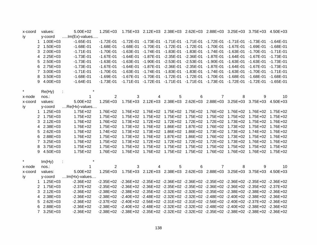
x-coord values: 5.00E+02 1.25E+03 1.75E+03 2.12E+03 2.38E+03 2.62E+03 2.88E+03 3.25E+03 3.75E+03 4.50E+03iy y-coord .....Im(Ex)-values.....

1 1.00E+03 -1.65E-01 -1.72E-01 -1.72E-01 -1.73E-01 -1.71E-01 -1.71E-01 -1.72E-01 -1.71E-01 -1.73E-01 -1.64E-012 1.50E+03 -1.68E-01 -1.68E-01 -1.68E-01 -1.70E-01 -1.72E-01 -1.72E-01 -1.70E-01 -1.67E-01 -1.69E-01 -1.68E-013 2.00E+03 -1.71E-01 -1.70E-01 -1.63E-01 -1.74E-01 -1.83E-01 -1.83E-01 -1.74E-01 -1.63E-01 -1.70E-01 -1.71E-014 2.25E+03 -1.73E-01 -1.67E-01 -1.64E-01 -1.87E-01 -2.35E-01 -2.36E-01 -1.87E-01 -1.64E-01 -1.67E-01 -1.73E-015 2.50E+03 -1.73E-01 -1.63E-01 -1.63E-01 -1.90E-01 -2.53E-01 -2.53E-01 -1.90E-01 -1.63E-01 -1.63E-01 -1.73E-016 2.75E+03 -1.73E-01 -1.67E-01 -1.64E-01 -1.87E-01 -2.36E-01 -2.35E-01 -1.87E-01 -1.64E-01 -1.67E-01 -1.73E-017 3.00E+03 -1.71E-01 -1.70E-01 -1.63E-01 -1.74E-01 -1.83E-01 -1.83E-01 -1.74E-01 -1.63E-01 -1.70E-01 -1.71E-018 3.50E+03 -1.68E-01 -1.69E-01 -1.67E-01 -1.70E-01 -1.72E-01 -1.72E-01 -1.70E-01 -1.68E-01 -1.68E-01 -1.68E-019 4.00E+03 -1.64E-01 -1.73E-01 -1.71E-01 -1.72E-01 -1.71E-01 -1.71E-01 -1.73E-01 -1.72E-01 -1.72E-01 -1.65E-01

* Re(Hy) : *x-node nos.: 1 2 3 4 5 6 7 8 9 10x-coord values: 5.00E+02 1.25E+03 1.75E+03 2.12E+03 2.38E+03 2.62E+03 2.88E+03 3.25E+03 3.75E+03 4.50E+03iy y-coord ....Re(Hx)-values....

1 1.25E+03 1.75E+02 1.76E+02 1.76E+02 1.76E+02 1.75E+02 1.75E+02 1.76E+02 1.76E+02 1.76E+02 1.75E+022 1.75E+03 1.75E+02 1.75E+02 1.75E+02 1.75E+02 1.75E+02 1.75E+02 1.75E+02 1.75E+02 1.75E+02 1.75E+023 2.12E+03 1.76E+02 1.76E+02 1.73E+02 1.72E+02 1.72E+02 1.72E+02 1.72E+02 1.73E+02 1.75E+02 1.76E+024 2.38E+03 1.76E+02 1.75E+02 1.73E+02 1.76E+02 1.86E+02 1.87E+02 1.76E+02 1.73E+02 1.75E+02 1.76E+025 2.62E+03 1.76E+02 1.74E+02 1.73E+02 1.73E+02 1.86E+02 1.86E+02 1.73E+02 1.73E+02 1.74E+02 1.76E+026 2.88E+03 1.76E+02 1.75E+02 1.73E+02 1.76E+02 1.87E+02 1.86E+02 1.76E+02 1.73E+02 1.75E+02 1.76E+027 3.25E+03 1.76E+02 1.75E+02 1.73E+02 1.72E+02 1.72E+02 1.72E+02 1.72E+02 1.73E+02 1.76E+02 1.76E+028 3.75E+03 1.75E+02 1.75E+02 1.75E+02 1.75E+02 1.75E+02 1.75E+02 1.75E+02 1.75E+02 1.75E+02 1.75E+029 4.50E+03 1.75E+02 1.76E+02 1.76E+02 1.76E+02 1.75E+02 1.75E+02 1.76E+02 1.76E+02 1.76E+02 1.75E+02

* Im(Hy) : *x-node nos.: 1 2 3 4 5 6 7 8 9 10x-coord values: 5.00E+02 1.25E+03 1.75E+03 2.12E+03 2.38E+03 2.62E+03 2.88E+03 3.25E+03 3.75E+03 4.50E+03iy y-coord ....Im(Hx)-values....

1 1.25E+03 -2.36E+02 -2.35E+02 -2.36E+02 -2.35E+02 -2.36E+02 -2.36E+02 -2.35E+02 -2.36E+02 -2.35E+02 -2.36E+022 1.75E+03 -2.37E+02 -2.35E+02 -2.36E+02 -2.36E+02 -2.35E+02 -2.35E+02 -2.36E+02 -2.36E+02 -2.35E+02 -2.37E+023 2.12E+03 -2.36E+02 -2.38E+02 -2.38E+02 -2.35E+02 -2.32E+02 -2.32E+02 -2.35E+02 -2.38E+02 -2.38E+02 -2.36E+024 2.38E+03 -2.36E+02 -2.38E+02 -2.40E+02 -2.48E+02 -2.32E+02 -2.32E+02 -2.48E+02 -2.40E+02 -2.38E+02 -2.36E+025 2.62E+03 -2.36E+02 -2.37E+02 -2.40E+02 -2.56E+02 -2.31E+02 -2.31E+02 -2.56E+02 -2.40E+02 -2.37E+02 -2.36E+026 2.88E+03 -2.36E+02 -2.38E+02 -2.40E+02 -2.48E+02 -2.32E+02 -2.32E+02 -2.48E+02 -2.40E+02 -2.38E+02 -2.36E+027 3.25E+03 -2.36E+02 -2.38E+02 -2.38E+02 -2.35E+02 -2.32E+02 -2.32E+02 -2.35E+02 -2.38E+02 -2.38E+02 -2.36E+02

138

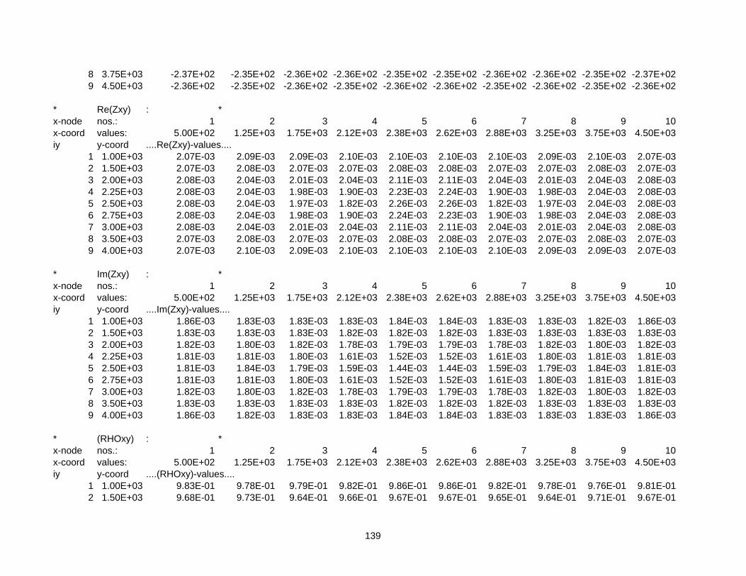
8 3.75E+03 -2.37E+02 -2.35E+02 -2.36E+02 -2.36E+02 -2.35E+02 -2.35E+02 -2.36E+02 -2.36E+02 -2.35E+02 -2.37E+029 4.50E+03 -2.36E+02 -2.35E+02 -2.36E+02 -2.35E+02 -2.36E+02 -2.36E+02 -2.35E+02 -2.36E+02 -2.35E+02 -2.36E+02

* Re(Zxy) : *x-node nos.: 1 2 3 4 5 6 7 8 9 10x-coord values: 5.00E+02 1.25E+03 1.75E+03 2.12E+03 2.38E+03 2.62E+03 2.88E+03 3.25E+03 3.75E+03 4.50E+03iy y-coord ....Re(Zxy)-values....

1 1.00E+03 2.07E-03 2.09E-03 2.09E-03 2.10E-03 2.10E-03 2.10E-03 2.10E-03 2.09E-03 2.10E-03 2.07E-032 1.50E+03 2.07E-03 2.08E-03 2.07E-03 2.07E-03 2.08E-03 2.08E-03 2.07E-03 2.07E-03 2.08E-03 2.07E-033 2.00E+03 2.08E-03 2.04E-03 2.01E-03 2.04E-03 2.11E-03 2.11E-03 2.04E-03 2.01E-03 2.04E-03 2.08E-034 2.25E+03 2.08E-03 2.04E-03 1.98E-03 1.90E-03 2.23E-03 2.24E-03 1.90E-03 1.98E-03 2.04E-03 2.08E-035 2.50E+03 2.08E-03 2.04E-03 1.97E-03 1.82E-03 2.26E-03 2.26E-03 1.82E-03 1.97E-03 2.04E-03 2.08E-036 2.75E+03 2.08E-03 2.04E-03 1.98E-03 1.90E-03 2.24E-03 2.23E-03 1.90E-03 1.98E-03 2.04E-03 2.08E-037 3.00E+03 2.08E-03 2.04E-03 2.01E-03 2.04E-03 2.11E-03 2.11E-03 2.04E-03 2.01E-03 2.04E-03 2.08E-038 3.50E+03 2.07E-03 2.08E-03 2.07E-03 2.07E-03 2.08E-03 2.08E-03 2.07E-03 2.07E-03 2.08E-03 2.07E-039 4.00E+03 2.07E-03 2.10E-03 2.09E-03 2.10E-03 2.10E-03 2.10E-03 2.10E-03 2.09E-03 2.09E-03 2.07E-03

* Im(Zxy) : *x-node nos.: 1 2 3 4 5 6 7 8 9 10x-coord values: 5.00E+02 1.25E+03 1.75E+03 2.12E+03 2.38E+03 2.62E+03 2.88E+03 3.25E+03 3.75E+03 4.50E+03iy y-coord ....Im(Zxy)-values....

1 1.00E+03 1.86E-03 1.83E-03 1.83E-03 1.83E-03 1.84E-03 1.84E-03 1.83E-03 1.83E-03 1.82E-03 1.86E-032 1.50E+03 1.83E-03 1.83E-03 1.83E-03 1.82E-03 1.82E-03 1.82E-03 1.83E-03 1.83E-03 1.83E-03 1.83E-033 2.00E+03 1.82E-03 1.80E-03 1.82E-03 1.78E-03 1.79E-03 1.79E-03 1.78E-03 1.82E-03 1.80E-03 1.82E-034 2.25E+03 1.81E-03 1.81E-03 1.80E-03 1.61E-03 1.52E-03 1.52E-03 1.61E-03 1.80E-03 1.81E-03 1.81E-035 2.50E+03 1.81E-03 1.84E-03 1.79E-03 1.59E-03 1.44E-03 1.44E-03 1.59E-03 1.79E-03 1.84E-03 1.81E-036 2.75E+03 1.81E-03 1.81E-03 1.80E-03 1.61E-03 1.52E-03 1.52E-03 1.61E-03 1.80E-03 1.81E-03 1.81E-037 3.00E+03 1.82E-03 1.80E-03 1.82E-03 1.78E-03 1.79E-03 1.79E-03 1.78E-03 1.82E-03 1.80E-03 1.82E-038 3.50E+03 1.83E-03 1.83E-03 1.83E-03 1.83E-03 1.82E-03 1.82E-03 1.82E-03 1.83E-03 1.83E-03 1.83E-039 4.00E+03 1.86E-03 1.82E-03 1.83E-03 1.83E-03 1.84E-03 1.84E-03 1.83E-03 1.83E-03 1.83E-03 1.86E-03

* (RHOxy) : *x-node nos.: 1 2 3 4 5 6 7 8 9 10x-coord values: 5.00E+02 1.25E+03 1.75E+03 2.12E+03 2.38E+03 2.62E+03 2.88E+03 3.25E+03 3.75E+03 4.50E+03iy y-coord ....(RHOxy)-values....

1 1.00E+03 9.83E-01 9.78E-01 9.79E-01 9.82E-01 9.86E-01 9.86E-01 9.82E-01 9.78E-01 9.76E-01 9.81E-012 1.50E+03 9.68E-01 9.73E-01 9.64E-01 9.66E-01 9.67E-01 9.67E-01 9.65E-01 9.64E-01 9.71E-01 9.67E-01

139

3 2.00E+03 9.65E-01 9.41E-01 9.34E-01 9.31E-01 9.70E-01 9.70E-01 9.31E-01 9.34E-01 9.41E-01 9.64E-014 2.25E+03 9.62E-01 9.40E-01 9.05E-01 7.87E-01 9.26E-01 9.24E-01 7.87E-01 9.05E-01 9.41E-01 9.62E-015 2.50E+03 9.62E-01 9.54E-01 9.00E-01 7.42E-01 9.07E-01 9.07E-01 7.42E-01 9.00E-01 9.54E-01 9.62E-016 2.75E+03 9.62E-01 9.41E-01 9.05E-01 7.87E-01 9.24E-01 9.26E-01 7.87E-01 9.05E-01 9.40E-01 9.62E-017 3.00E+03 9.64E-01 9.41E-01 9.34E-01 9.31E-01 9.70E-01 9.70E-01 9.31E-01 9.34E-01 9.41E-01 9.65E-018 3.50E+03 9.67E-01 9.71E-01 9.64E-01 9.65E-01 9.67E-01 9.67E-01 9.66E-01 9.64E-01 9.73E-01 9.68E-019 4.00E+03 9.81E-01 9.76E-01 9.78E-01 9.82E-01 9.86E-01 9.86E-01 9.82E-01 9.79E-01 9.78E-01 9.83E-01

* PHASExy : *x-node nos.: 1 2 3 4 5 6 7 8 9 10x-coord values: 5.00E+02 1.25E+03 1.75E+03 2.12E+03 2.38E+03 2.62E+03 2.88E+03 3.25E+03 3.75E+03 4.50E+03iy y-coord ....PHASExy-values....

1 1.00E+03 4.19E+01 4.11E+01 4.11E+01 4.10E+01 4.13E+01 4.13E+01 4.11E+01 4.12E+01 4.10E+01 4.19E+012 1.50E+03 4.15E+01 4.14E+01 4.15E+01 4.13E+01 4.11E+01 4.12E+01 4.14E+01 4.15E+01 4.14E+01 4.16E+013 2.00E+03 4.12E+01 4.14E+01 4.21E+01 4.11E+01 4.02E+01 4.02E+01 4.11E+01 4.22E+01 4.14E+01 4.12E+014 2.25E+03 4.10E+01 4.16E+01 4.22E+01 4.03E+01 3.43E+01 3.41E+01 4.03E+01 4.22E+01 4.17E+01 4.10E+015 2.50E+03 4.10E+01 4.20E+01 4.23E+01 4.12E+01 3.25E+01 3.25E+01 4.12E+01 4.23E+01 4.20E+01 4.10E+016 2.75E+03 4.10E+01 4.17E+01 4.22E+01 4.03E+01 3.41E+01 3.43E+01 4.03E+01 4.22E+01 4.16E+01 4.10E+017 3.00E+03 4.12E+01 4.14E+01 4.22E+01 4.11E+01 4.02E+01 4.02E+01 4.11E+01 4.21E+01 4.14E+01 4.12E+018 3.50E+03 4.16E+01 4.14E+01 4.15E+01 4.14E+01 4.12E+01 4.11E+01 4.13E+01 4.15E+01 4.14E+01 4.15E+019 4.00E+03 4.19E+01 4.10E+01 4.12E+01 4.11E+01 4.13E+01 4.13E+01 4.10E+01 4.11E+01 4.11E+01 4.19E+01

140

141

Output_time.dat

date time_mainstart= 20090823 105149.921 date and time start_eigenstep1= 20090823 105149.984 date and time end_eigenstep1= 20090823 105302.953 date and time start_eigenstep2= 20090823 105302.953 date and time end_eigenstep2= 20090823 105302.953 date and time start_dlahqr= 20090823 105303.015 date and time end_dlahqr= 20090823 105319.015 date time_mainend= 20090823 105409.328

143

REFERENCES

Abdul Azeez, K. K., and Harinarayana, T., 2007. Magnetotelluric evidence of potential

geothermal resource in Puga, Ladakh, NW Himalaya. Current Sci., 93, 323-329.

Adam, A., 1997. Magnetotelluric phase anisotropy above extensional structures of the

Neogene Pannonian Basin. J. Geomag. Geoelec., 49, 1549-1557.

Arnoldi, W. E., 1951. The principle of minimized iteration in the solution of the matrix

eigenproblem. Quart. Appl. Math., 9, 17-29.

Asaue, H., Koike, K., Yoshinaga, T., and Takakura, S., 2006. Magnetotelluric resistivity

modeling for 3D characterization of geothermal reservoirs in the Western side of

Mt. Aso, SW Japan. J. App. Geophys., 18, 296-312.

Avdeev, D. B., 2005. Three-dimensional electromagnetic modelling and inversion from

theory to application. Sur. Geophys., 26, 767-799.

Backus, G. E., and Gilbert, J. E., 1970. Uniqueness in the inversion of inaccurate gross

earth data. Phil. Trans. Roy. Soc. London, 266, 123-192.

Baglama, J., Calvetti, D., and Reichel, L., 1996. Iterative methods for the computation of a

few eigenvalues of a large symmetric matrix. BIT, 36, 400-421.

Baglama, J., Calvetti, D., and Reichel, L., 1998. Fast leja points. Elect. Trans. Num. Anal.,

7, 124-140.

Barrett, R., Berry, M., Chan, T. F., Demmel, J., Donato, J., Dongarra, J., Eijkhout, V.,

Pozo, R., Romine, C., and van der Vorst, H., 1994. Templates for the solution of

linear systems: building blocks for iterative methods. Society for industrial and

applied mathematics, Philadelphia, PA.

144

Beattie, C. A., Embree, M., and Sorensen, D. C., 2005. Convergence of polynomial restart

krylov methods for eigenvalue computations. SIAM review, 47, 492-515.

Berdichevsky, M. N., and Zhdanov, M. S., 1984. Advanced theory of deep geomagnetic

sounding. Elsevier, Amsterdam, pp. 408.

Bhattacharya, B. B., and Sen, M. K., 1981. Depth of investigation of collinear electrode

arrays over homogeneous, anisotropic half-space in direct current method.

Geophys., 46, 768-780.

Bhattacharya, B. B., Mukherjee, D. S., and Chatterjee, D., 1983. Enhancement of EM

anamoly: A circuit theory approach. Geophys., 48, 1248-1251.

Blome, M., Maurer, H. R., and Schmidt, K., 2009. Advances in three-dimensional

geoelectric forward solver techniques. Geophys. J. Int., 176, 740-752.

Born, M., and Wolf, E., 2005. Principles of optics, 7th edition. Cambridge University Press,

UK, pp. 952.

Brewitt-Taylor, C. R., and Weaver, J. T., 1976. On the finite difference solution of two-

dimensional induction problems. Geophys. J. R. Atsr. Soc., 47, 375-396.

Brezinski, C., Redivo-Zaglia, M., and Sadok, H., 2001. The matrix and polynomial

approaches to Lanczos-type algorithms. J. Comp. Appl. Math., 123, 241-260.

Cagniard, L., 1953. Basic theory of the magnetotelluric method of geophysical prospecting.

Geophys., 18, 605-635.

Calvetti, D., Reichel, L., and Sorensen, D. C., 1994. An implicitly restarted Lanczos

method for large symmetric eigenvalue problems. Elect. Trans. Num. Anal., 2, 1-

21.

145

Cantwell, T., 1960. Detection and analysis of low frequency magnetotelluric signal. Ph.D.

Thesis, Dept. of Geol. and Geophys., M. L. T., Cambridge, Mass.

Cerv, V., and Pek, J., 1990. Modeling and analysis of electromagnetic fields in 3D

inhomogeneous media. Sur. Geophys., 11, 205-229.

Cerv, V., Menvielle, M., and Pek, J., 2007. Stochastic interpretation of magnetotelluric

data, comparison of methods. Ann. Geophys., 50, 7-19.

Changsheng, L., Zhengyong, R., Jingtian, T., and Yan, Y., 2008. Three-dimensional

magnetotellurics modeling using edge based finite-element unstructured meshes.

App. Geophys., 5, 170-180.

Chen, C., C., Chen, C., Chiang, C., Shu, H., Chiu, W., Unsworth, M. J., and Bertrand, E.,

2007. Crustal resistivity anomalies beneath Central Taiwan imaged by a broadband

magnetotelluric transect. Terr. Atmos. Ocean. Sci., 18, 19-30.

Chen, L., Booker, J. R., Jones, A. G., Wu, N., Unsworth, M. J., Wenbo, W., and Tan, H.,

1996. Electrically conductive crust in southern Tibet from INDEPTH

magnetotelluric surveying. Sci., 274, 1694-1696.

Chen, P., Hou, Z., and Fan, G., 1998. Three-dimensional topographic responses in MT

using finite difference method. Acta Seis. Sinica, 11, 631-635.

Coggon, J. H., 1971. Electromagnetic and electrical modeling by the finite element method.

Geophys., 36, 132-155.

Commer, M., and Newman, G. A., 2008. New advances in three-dimensional controlled-

source electromagnetic inversion. Geophys. J. Int., 172, 513-535.

Constable, S., and Cox, C. S., 1996. Marine controlled source electromagnetic sounding.

The PEGASUS experiment. J. Geophys. Res., 101, 5519-5530.

146

Constable, S., and Srnka, L. J., 2007. An introduction to marine controlled-source

electromagnetic methods for hydrocarbon exploration. Geophys., 72, WA3-WA12.

Constable, S., and Weiss, C. J., 2006. Mapping thin resistors and hydrocarbons with marine

EM methods: Insights from 1D modeling. Geophys., 71, G43-G51.

Constable, S., Orange, A., Hoversten, G. M., and Morrison, H. F., 1998. Marine

magnetollurics for petroleum exploration. A seafloor instrument system. Geophys.,

63, 816-825.

Cox, C. S., 1981. On the electrical conductivity of the oceanic lithosphere. Phys. Earth

Planet. Int., 25, 196-201.

Cox, C. S., Filloux, J. H., Gough, D. I., Larson, J. C., Poehls, K. A., Von Herzen, R. P., and

Winter, R., 1980. Atlantic lithosphere sounding. J. Geomag. Geoelec., 32, Suppl. I,

SI 13– SI 32.

Cullum, J. K., and Willoughby, R. A., 1985. Lanczos algorithms for large symmetric

eigenvalue computations; Vol. I, Theory. Birkhauser, Printed in Germany, pp. 268.

Cullum, J. K., and Willoughby, R. A., 1985. Lanczos algorithms for large symmetric

eigenvalue computations; Vol. II, Programs. Birkhauser, Printed in Germany, pp.

496.

Daniel, J., Gragg, W. B., Kaufman, L., and Stewart, G. W., 1976. Reorthogonalization and

stable algorithms for updating the Gram-Schmidt QR factorization. Math. Comp.,

30, 772-795.

Das, U. C., and Verma, S. K., 1981. Numerical considerations on computing the EM

response of three dimensional inhomogeneities in a layered earth. Geophys. J. R.

Astr. Soc., 66, 733-740.

147

Das, U. C., and Verma, S. K., 1982. Electromagnetic response of an arbitrary straped three

dimensional conductor in a layered earth - numerical results. Geophys. J. R. Astr.

Soc., 68, 55-66.

deGroot-Hedlin, C., and Constable, S., 1990. Occam’s inversion to generate models form

magnetotelluric data. Geophys., 55, 1613-1624.

deGroot-Hedlin, C., and Constable, S., 2004. Inversion of magnetotelluric data for 2D

structure with sharp resistivity contrast. Geophys., 69, 78-86.

de Lima, O. A. L., Sato, H. K., and Porsani, M. J., 1995. Imaging industrial contaminant

plumes with resistivity techniques. J. App. Geophys., 34, 93-108.

Dmitriev, V. I., and Berdichevsky, M. N., 1979. Fundamental model of magnetotelluric

sounding. Proc. IEEE, 67, 1034-1043.

Druskin, V., and Knizhnerman, L., 1994. Spectral approach to solving three-dimensional

diffusion Maxwell’s equations in the time and frequency domains. Radio Sci., 29,

937-953.

Druskin, V. L., Knizhnerman, L. A., and Lee, P., 1999. New spectral Lanczos

decomposition method for induction modeling in arbitrary 3-D geometry. Geophys.,

64, 701-706.

Duff, I. S., and Scott, J. A., 1993. Computing selected eigenvalues of sparse unsymmetric

matrices using subspace iteration. Internal Report, RAL-91-056.

Eidsmo, T., Ellingsrud, S., MacGregor, L. M., Constable, S., Sinha, M. C., Johanson, S.,

Kong, F. N., and Westerdahl, H., 2002. Sea Bed Logging (SBL), a new method for

remote and direct identification of hydrocarbon filled layers in deepwater areas.

First Break, 20, 144-152.

148

Ellingsrud, S., Eidsmo, T., Johansen, S., Sinha, M. C., MacGregor, L. M., and Constable,

S., 2002. Remote sensing of hydrocarbon layers by seabed logging (SBL): Results

from a cruise offshore Angola. The Leading Edge, 21, 972-982.

Emad, N., Petiton, S., and Edjlali, G., 2005. Multiple explicitly restarted Arnoldi method

for solving large eigenproblems. SIAm J. Sci, Comp., 27, 253-277.

Ericsson, T., and Ruhe, A., 1980. The spectral transformation Lanczos method for the

numerical solution of large sparse generalized symmetric eigenvalue problems.

Math. Comp., 35, 1251-1268.

Farquharson, C. G., and Oldenburg, D. W., 2002. Three-dimensional forward- modeling

and inversion algorithms for magnetotelluric data. 16th workshop on

electromagnetic induction on the earth, June 16-22, College of Santa Fe, Santa Fe,

New Mexico, USA.

Fomenko, E. Y., and Mogi, T., 2002. A new computation method for a staggered grid of

3D EM field conservative modeling. Earth Planets Space, 54, 499-509.

Forsythe, G. E. and Wasow, W. A., 1964. Finite difference method for partial differential

equations. Wiley, New York, pp. 444.

Fox, L., and Ingerov, O., 2007. Natural source EM for offshore hydrocarbon detection

offers potential cost savings. First Break, 25, 87-96.

Giraud, L., Langou, J., and Rozloznik, M., 2003. On the loss of orthogonality in the Gram-

Schmidt orthogonalization process. CERFACS Technical Report No. TR/PA/03/25.

URL http://www.cerfacs.fr/algor/reports/2003/TR_PA_03_25.pdf.

Golub, G. H., and VanLoan, C. F., 1983. Matrix computations. The John Hopkins

University Press, Baltimore, Maryland.

149

Grant, F. S., and West, G. F., 1965. Interpretation theory in applied geophysics. McGraw-

HiliBook Company, New York, pp. 584.

Groom, R. W., and Bailey, R. C., 1989. Decomposition of magnetotelluric impedance

tensors in the presence of local three-dimensional galvanic distortion. J. Geophys.

Res., 94, 1913-1925.

Gupta, P. K., Bennett, L. A., and Raiche, A. P., 1987. Hybrid calculation of the three-

dimensional electromagnetic response of buried conductors. Geophys., 52, 301-306.

Gupta, P. K., Niwas, S., and Gaur, V. K., 1996. Straightforward inversion scheme (SIS) for

one-dimensional magnetotelluric data. J. Earth Sys. Sci., 105, 413-429.

Gupta, P. K., Niwas, S., and Gaur, V. K., 1997. Straightforward inversion of vertical

electrical sounding data. Geophys., 62, 775-785.

Harinarayana, T., Murthy, D. N., Eknath Rao, S. P., Manoj, C., Veeraswamy, K.,

Naganjaneyulu, K., Abdul Azeez, K. K., Sastry, R. S., and Virupakshi, G., 2002.

Magnetotelluric field investigations in Puga geothermal region, Jammu and

Kashmir, India: 1-D modeling results. Geotherm. Resour. Counc. Trans., 26, 393-

397.

Hernandez, V., Roman, J. E., and Tomas, A., 2007. Evaluation of several variants of

explicitly restarted Lanczos eigensolvers and their parallel implementations. LNCS,

4395, 403-416.

Hetmaniuk, U., and Lehoucq, R. B., 2006. Uniform accuracy of eigenpairs from a shift-

invert Lanczos method. SIAM J. Matrix Anal. Appl., 28, 927-948.

Hildebrand, F. B., 1974. Introduction to numerical analysis, Tata-McGraw Hill, New

Delhi, pp. 669.

150

Hochstenbach, M. E., 2003. Subspace methods for eigenvalue problems. Ph. D. Thesis,

Department of Information and Computing Sciences, Utrecht University,

Nederlands.

Hohmann, G. W., 1975. Three-dimensional induced polarization and electromagnetic

modeling. Geophys., 40, 309-324.

Hohmann, G. W., 1983. Three-dimensional EM modeling. Geophys. Sur., 6, 27-53.

Hohmann, G. W., and Ting, S. C., 1978, Three-dimensional magnetotelhuic modeling: ESL

Final Rep. 77-15, DOE contract EY-76-S-07- 1601, July, pp. 48.

Hoover, D. B., Long, C. L., and Senterfit, R. M., 1978. Some results from

audiomagnetotellurics investigations in geothermal areas. Geophys., 43, 1501-1514.

Ipsen, I. C. F., and Meyer, C. D., 1998. The idea behind Krylov methods. Am. Math. Mon.,

105, 889-899.

Israil, M., Tyagi, D. K., Gupta, P. K., and Niwas, S., 2008. Magnetotelluric investigations

for imaging electrical structure of Garhwal Himalayan corridor, Uttarakhand, India.

J. Earth. Syst. Sci., 117, 189-200.

Jackson, J. D., 1975. Classical electrodynamics. John Wiley and Sons, New York.

Jacobs, D. A. H., 1981a. The exploitation of sparsity by iterative methods. In: Sparse

matrices and their uses, Ian S. Duff (Ed.), Springer-Verlag, 191-221.

Jacobs, D. A. H., 1981b. Preconditioned conjugate gradient algorithm for solving finite

difference system. In: Sparse matrices and their uses. Ian S. Duff (Ed.), Springer-

Verlag, 509-535.

151

Johansen, S. E., Amundsen, H. E. F., Røsten, T., Ellingsrud, S., Eidesmo, T., and Bhuyian,

A. H., 2005. Subsurface hydrocarbons detected by electromagnetic sounding. First

Break, 23, 31-36.

Jones, F. W. and Pascoe, L. J., 1971. A general computer program to determine the

perturbation of alternating electric currents in a two-dimensional model of a region

of uniform conductivity with an embedded inhomogeneity. Geophys. J. R. Astr.

Soc., 24, 3-30.

Jones, F. W., and Pascoe, L. J., 1972. The perturbation of geomagnetic fields by three-

dimensional conductive inhomoginities. Geophys. J. R. Astr. Soc., 27, 479-485.

Jones, F. W., and Vozoff, K., 1978. The calculation of magnetotelluric quantities for three-

dimensional conductivity inhomogeneities. Geophys., 43, 1167-1175.

Joubert, W., 1992. Lanczos methods for the solution of nonsymmetric system of linear

equations. Siam J. Matrix Anal. Appl., 13, 926-943.

Kaufman, A. A., and Keller, G. V., 1981. The magnetotelluric sounding method. Elsevier,

Amsterdam.

Khattri, K. N., 1992. Local seismic investigations in the Garhwal-Kumaun Himalaya.

Mem. Geol. Soc. India, 23, 45-66.

Kong, F. N., Westerdahl, H., Ellingsrud, S., Eidesmo, T., and Johansen, J., 2002. ‘Seabed

logging’: A possible direct hydrocarbon indicator for deep sea prospects using EM

energy. Oil and Gas Journal, 100, 30-38.

Kumar, R., Ghosh, S. K., Sangode, S. J., and Thakur, V. C., 2002. manifestation of Intra-

Foreland thrusting in the Neogene Himalaya foreland basin fill. J. Geo. Soc. India,

59, 547-560.

152

Lagios, E., Galanapoulos, D., Hobbs, B. A., Dawes, G. J. K., 2002. Two-dimensional

magnetotelluric modeling of the Kos Island geothermal region (Greece).

Tectonophys., 287, 157-172.

Lanczos, C., 1950. An iterative method for the solution of the eigenvalue problem of linear

differential and integral operators. J. Res. Natl. Bur. Stand., 45, 225-280.

Langou, M. J., 2003. Iterative methods for solving linear systems with multiple right hand

sides. Ph.D. Dissertation, INSA, Toulouse, France.

Ledo, J., 2005. 2-D verses 3-D magnetotelluric data interpretation. Sur. Geophys., 26, 511-

543.

Lee, K. H., Pridmore, D. F., and Morrison H. F., 1981. A hybrid three-dimensional

electromagnetic modeling scheme. Geophys., 46, 796-805.

Lee, T. J., Song, Y., and Uchida, T., 2007. Three-dimensional magnetotelluric surveys for

geothermal development in Pohang, Korea. Expol. Geophys., 38, 89-97.

Lehoucq, R. B., 1997. Truncated QR algorithms and the solution of large-scale eigenvalue

problems. Preprint MCS-P648-0297, Mathematics and Computer Science Division,

Argonne National Laboratory, Argonne, Ill.

Lehoucq, R. B., and Scott, J. A., 1996. An evaluation of Arnoldi based software for sparse

nonsymmetric eigenproblems. Internal Report, RAL-TR-96-023.

Lehoucq, R. B., and Scott, J. A., 1997. Implicitly restarted Arnoldi methods and

eigenvalues of the discretized Navier Stokes equations. SIAM J. Matrix Anal.

Appl., 23, 551-562.

Lehoucq, R. B., and Sorensen, D. C., 1996. Deflation techniques for an implicitly re-started

Arnoldi iteration. SIAM J. matrix Anal. Appl., 17, 789-821.

153

Lehoucq, R. B., Sorensen, D. C., and Yang, C., 1997. ARPACK Users' Guide: Solution of

Large Scale Eigenvalue Problems with Implicitly Restarted Arnoldi Methods.

http://www.caam.rice.edu/software/ARPACK/UG/ug.html.

Livelybrooks, D., 1993. Program 3D feem: a multidimensional electromagnetic finite

element model. Geophys. J. Int., 114, 443-458.

MacGregor, L., and Sinha, S., 2000. Use of marine controlled-source electromagnetic

sounding for sub-basalt exploration. Geophys. Prosp., 48, 1091-1106.

MacGregor, L., Sinha, M., and Constable, S., 2001. Electrical resistivity structure of the

Valu Fa Ridge, Lau Basin, from marine controlled-source electromagnetic

sounding. Geophys. J. Int., 146, 217-236.

Mackie, R. L., Madden, T. R., and Wannamaker, P. E., 1993. Three-dimensional

magnetotelluric modeling using difference equations- Theory and comparisons to

integral equation solutions. Geophys., 58, 215-226.

Madden, T. R., and Mackie, R. L., 1989. Three-Dimensional Magnetotelluric Modeling

and Inversion. Proceedings of the IEEE, 77, 318-333.

Manteuffel, T. A., 1978. Adaptive procedure for estimating parameters for the

nonsymmetric Tchebyshev iteration. Numer. Math., 31, 183-208.

Mauro, D. D., Volpi, G., Manzella, A., Zaja, A., Praticelli, N., Cerv, V., Pek, J., and Santis,

A. D., 1999. Magnetotelluric investigations of the seismically active region of

Northwest Bohemia: preliminary results. Ann. Geofis., 42, 39-48.

McNeice, G. W., and Jones, A. G., 2001. Mutisite, mutifrequency tensor decomposition of

magnetotelluric data. Geophys., 66, 158-173.

154

Meerbergen, K., Scott, J., 2000. The design of a block rational Lanczos code with partial

reorthogonalization and implicit restarting, RAL-TR-2000-011.

Meerbergen, K., Spence, A., and Roose, D., 1994. Shift-invert and Cayley transforms for

detection of rightmost eigenvalues of nonsymmetric matrices. BIT, 34, 409-423.

Meurant, G., and Strakos, Z., 2006. The Lanczos and conjugate gradient algorithms in

finite precision arithmetic. Acta Num., 15, 471-542.

Mitchell, A. R., and Griffiths, D. F., 1980. The finite difference method in partial

differential equations. Wiley-Interscience publication, Chichester, Wiley.

Mitra, R., 1973. Computer techniques for electromagnetics. Pergamon, New York.

Mitra, R., 1975. Numerical and asymptotic techniques in electromagnetics. Springer-

Verlag, New York.

Mitsuhata, Y., and Uchida, T., 2004, Three-dimensional magnetotelluric modeling using

the T-Ω finite element method. Geophys., 69, 108-119.

Mogi, T., 1996. Three-dimensional modeling of magnetotelluric data using finite element

method. J. App. Geophys., 35, 185-189.

Monk, P., and Suli, E., 1994. A convergence analysis of Yee’s scheme on nonuniform

grids. SIAM J. Num. Anal., 31, 393-412.

Morgan, M. A., (Ed.), 1990. Finite element and finite difference methods in

electromagnetic scattering. Elsevier, New York.

Morgan, R. B., 1996. On restarting the Arnoldi method for large nonsymmetric eigenvalue

problems. Math. Comp., 65, 1213-1230.

Morgan, R. B., and Zeng, M., 2006. A harmonic restarted Arnoldi algorithm for calculating

eigenvalues and determining multiplicity. Linear Alg. Appl., 415, 96-113.

155

Morse, P. M., and Feshbach, H., 1953. Methods of theoretical physics. McGraw-Hill Book

Co., Inc., Tokyo.

Nabighian, M. N. (Ed.), 1988. Electromagnetic methods in applied geophysics, Vol. I,

Theory. Soc. Expl. Geophys.

Nabighian, M. N. (Ed.), 1991. Electromagnetic methods in applied geophysics, Vol. II,

Applications. Soc. Expl. Geophys.

Najman, Y., 2006. The detrital record of orogenesis: a review of approaches and techniques

used in the Himalayan Sedimentary Basins. Earth Sci. Rev., 74, 1-72.

Nam, M. J., Kim, H. J., Song, Y., Lee, T. J., Son, J.-S., and Suh, J. H., 2007. 3D

magnetotelluric modelling including surface topography. Geophys. Pros., 55, 277-

287.

Newman, G. A., and Alumbaugh, D. L., 1997. 3D electromagnetic modeling using

staggered finite differences. IEEE: Geoscience and Remote Sensing, 2, 929-932.

Oldenburg, D. W., 1979. One-dimensional inversion of natural source magnetotelluric

observations. Geophys., 44, 1218-1244.

Oldenburg, D. W., and Ellis, R. G., 1993. Efficient inversion of magnetotelluric data in

two-dimensions. Phys. Earth Planet. Int., 81, 177-200.

Paige, C. C., 1970. Practical use of the symmetric Lanczos process with re-

orthogonalization. BIT, 10, 183-195.

Pak, J., 1985. Linearization methods of interpreting magnetotelluric and magnetic variation

data. Travaux Inst. Geophys. Acad. Tchecosl. Sci., 609, 199-326.

156

Pandey, R. K., and Bhattacharya, B. B., 1983. Correction factor for determining depth to

the basement from H-type magnetotelluric sounding curves. GSI special Publication

Series, 2, 505 – 512.

Park, J., and Chave, A. D., 1984. On the estimation of magnetotelluric response functions

using the singular value decomposition. Geophys. J. R. Atsr. Soc., 77, 683-709.

Park, S. K. and Torres-Verdin, C., 1988. A Systematic Approach to the Interpretation of

Magnetotelluric Data in Volcanic Environments with Applications to the Quest for

Magma in Long Valley, California. J. Geophys. Res., 93, 13265-13283.

Parker, R. L., 1977. Understanding inverse theory. Annu. Rev. Earth Planet. Sci., 5, 35-64.

Parlett, B. N., and Scott, D. S., 1979. The Lanczos algorithm with selective

orthogonalization. Math. Comp., 33, 311-328.

Patricia, P. D. L., Francesco, L. E., Berthold, K., and Sergio, F., 2002. Magnetotelluric

studies of the Caldas Novas geothermal reservoir, Brazil. J. App. Geophys., 49, 33-

46.

Pedersen, L. B., and Engels, M., 2005. Routine 2D inversion of magnetotelluric data using

the determinant of impedance tensor. Geophys., 70, G33-G41.

Pellerin, L., Johnston, J. M., and Hohmann, G. W., 1996. A numerical evaluation of

electromagnetic methods in geothermal exploration. Geophys., 61, 121-130.

Petrick, W. R., 2005. A new passive technique to monitor and discover agricultural

groundwater resources. Industrial Imaging Co., Inc., Salt Lake city, UT 84103.

Porsani, M. J., and Ulrych, T. J., 1989. Discrete convolution by means of forward and

backward modeling. IEEE Trans. Acous. Speech and signal Proc., 37, 1680-1686.

Porstendorfer, G., 1975. Principles of magnetotelluric prospecthig. Bomtraeger, Berlin.

157

Pous, J., Ledo, J., Marcuello, A., and Daignières, M., 2007. Electrical resistivity model of

the crust and upper mantle from a magnetotelluric survey through the central

Pyrenees. Geophys. J. Int., 121, 750-762.

Press, W. H., Teukolsky, S. A., Vellerling, W. T., and Flannery, B. P., 1993. Numerical

recipes in FORTRAN. Second Edition, in arrangement with Cambridge University

Press, Foundation Books, Delhi, India.

Price, A. T., 1962. The theory of magnetotelluric methods when the source field is

considered. J. Geophys. Res., 67, 1907-1918.

Pridmore, D. F., Hohmann, G. W., Ward, S. H., and Sill, W. R., 1981. An investigation of

finite element modeling for electrical and electromagnetic data in three-dimensions.

Geophys., 46, 1009-1024.

Raiche, A. P., 1974. An integral equation approach to three-dimensional modeling.

Geophys. J. R. Astr. Soc., 36, 363-376.

Rao, I. B. R. R., Chary, M. V., and Mathur, R. R., 2003. EM studies over suspected seismic

zones in peninsular India, Mem. Geol. Soc. .India, 54, 23-42.

Rao, I. B. R. R., Nagendra, R., Rao, S. L. N., and Venkatramaiah , J., 2008. Very low

frequency electromagnetic prospecting method-A few field applications in India. J.

Earth Syst. Sci., 92, 165-177.

Rastogi, A., Gupta, P. K., and Niwas, S., 1997. Multigrid inversion of two-dimensional EM

data using bi-conjugate gradient method. J. Assoc. Expl. Geophys., India, 18, 43-

49.

158

Reddy, I. K., Rankin, D., and Phillips, R. J., 1977. Three-dimensional modeling in

magnetotelluric and magnetic variational sounding. Geophys. J. R. Astr. Soc., 51,

313-325.

Rikitake, T., 1966. Electromagnetism and the earth's interior. Elsevier, Amsterdam, pp.

308.

Rokityansky, I. I., 1982. Geoelectromagnetic investigations of the earth's crust and mantle.

Springer-Verlag, Berlin, pp. 381.

Ruhe, A., 1979. Implementation aspects of band Lanczos algorithms for computation of

eigenvalues of large sparse symmetric matrices. Math. Comp., 33,680-687.

Saad, Y., 1980. Variations on Arnoldi’s method for computing eigenelements of large

unsymmetric matrices. Lin. Alg. Appl., 34, 269-295.

Saad, Y., 1984. Chebyshev acceleration technique for solving nonsymmetric eigenvalue

problems. Math. Comp., 42, 567-588.

Saad, Y., 1994. SPARSKIT: A basic tool kit for sparse matrix calculations, version 2.

Technical report, CSRD, University of Illinois and RIACS (NASA Ames Research

Centre). URL http:// www-users.cs.umn.edu/ saad/softwares /SPARSKIT/

sparskit.html.

Sarkar, T. K., Siarkiewicz, K. R., and Stratton, R. F., 1981. Survey of numerical methods

for solution of large system of linear equations for electromagnetic field problems.

IEEE Trans. Antennas Propagat., AP-29, 847-856.

Sasaki, Y., 2001. Full 3-D inversion of electromagnetic data on PC. J. App. Geophys., 46,

45-54.

159

Schnegg, P.-A., 1999. A computing method for 3D magnetotelluric modelling directed by

polynomials. Earth Planets Space, 51, 1005-1012.

Scott, J. A., 1993. An Arnoldi code for computing selected eigenvalues of sparse real

unsynmmetric matrices. Council for the Central Laboratory of the Research

Councils, Internal Report RAL-93-097, Rutherford Appleton Laboratory, Chilton

Didcot, Oxfordshire, UK.

Semenov, V. Y., Adam, A., Jozwiak, W., Ladanyvskyy, B., Logvinov, I. M., Pek, J.,

Pushkarev, P., Vozar, J. and Experimental Team of CEMES, 2008. Electrical

structure of the upper mantle beneath Central Europe: Results of the CEMES

project. Acta Geophys., 56, 957-981.

Shalivahan, Sinharay, R. K., and Bhattachary, B. B., 2006. Remote reference (RR)

magnetotelluric (MT) impedance estimation of wideband data using hybrid

algorihm. J. Geophys. Res., 111, B11103.

Shi, X., Utada, H., Wang, J., Siripunvaraporn, W., and Wu, W., 2004. Three dimensional

magnetotelluric forward modeling using vector finite element method combined

with divergence corrections (VFE++). IAGA WG 1.2 on Electromagnetic Induction

in the Earth, Proceedings of the 17th Workshop, Hyderabad, India.

Singh, R. P., and Lal, T., 1980a. Wave-tilt characteristics of EM waves over a

homogeneous earth model. IEEE Trans. on Geoscience and Remote Sensing, GE-

18, 285-288.

Singh, R. P., and Lal, T., 1980b. Reflection characteristics of EM waves over

homogeneous earth model. Ann. di Geofis., 33, 247-258.

160

Singh, R. P., Kant, Y., and Rastogi, A., 1992. Magnetotelluric sounding in indo-Gangatic

plains and Himalayan foothills region. Indian J. Pet. Geol., 1, 258-271.

Siripunvaraporn, W., Egbert, G., and Lenbury, Y., 2002. Numerical accuracy of

magnetotelluric modeling: A comparison of finite difference approximations. Earth

Planets Space, 54, 721-725.

Smith, J. T., 1996a. Conservative modeling of 3-D electromagnetic fields, Part I: Properties

and error analysis. Geophys., 61, 1308-1318.

Smith, J. T., 1996b. Conservative modeling of 3-D electromagnetic fields, Part II:

Biconjugate gradient solution and an accelerator. Geophys., 61, 1319-1324.

Smith, J. T., and Booker, J. R., 1991. Rapid inversion of two- and three-dimensional

magneto-telluric data. J. Geophys. Res., 96, 3905-3922.

Smythe, W. R., 1950. Static and dynamic electricity. McGraw-Hill Book Co., Inc., Tokyo,

pp. 616.

Sommerfield, A., 1909. Propagation of waves in wireless telegraphy. Ann. Phys.,

(Germany), 28, 665–736.

Sommerfield, A., 1926. Propagation of waves in wireless telegraphy. Ann. Phys.,

(Germany), 81, 1135–1153.

Sorensen, D. C., 1992. Implicit application of polynomial filters in a k-step Arnoldi

method. J. Matrix Anal. Appl., 13, 357-385.

Sorensen, D. C., 1995. Implicitly restarted Arnoldi/Lanczos method for large scale

eigenvalue calculations. Parallel Numerical Algorithms: Proceedings of an

ICASE/LaRC Workshop, Edited by Keyes, D. E., A. Sameh, A., and

Venkatakrishnan, V., Kluwer.

161

Sorkhabi, R. B., Stump, E., Foland, K., and Jain, A. K., 1999. Tectonic and cooling history

of the Garhwal Higher Himalaya (Bhagirathi Valley): constraints from

thermochronological data. Gondwana Research Group Memoir, 6, 217-235.

Srivastava, S. P., Douglass, J. L., and Ward, S. H., 1963. The application of

magnetotelluric and telluric methods in central Alberta. Geophys., 28, 426-466.

Stratton, J. A., 1941. Electromagnetic theory. McGraw-Hill Book Co., Inc., Tokyo.

Stuntebeck, C., 2003. Three-dimensional electromagnetic modeling by free-decay mode

superposition. Ph.D. Thesis, Braunschweig University, Germany.

Tabbagh, A., 1985. The response of a three-dimensional magnetic and conductive body in

shallow depth electromagnetic prospecting. Geophys. J. R. Astr. Soc., 81, 215-230.

Taflove, A., 1995. Computational electrodynamics: The finite-differentiation time-domain

method. Artech House, Inc., Morwood, pp. 599.

Tezkan, B., 1994a. On the detectability of a highly conductive layer in the upper mantle

beneath the Black Forest crystalline using magnetotelluric methods. Geophys. J.

Int., 118, 185-200.

Tezkan, B., Hördt, A., and Gobashy, M., 2000. Two dimensional inversion of

radiomagnetotelluric data: selected case histories for waste site exploration. J. App.

Geophys., 44, 237-256.

Tikhonov, A. N., 1950. On investigation of electrical characteristics of deep strata of

Earth’s crust (in Russian). Dokl. Acad. Nauk USSR, 73, 295-297.

Ting, S. C., and Hohmann, G. W., 1981. Integral equation modeling of three-dimensional

magnetotelluric response. Geophys., 46, 182-197.

162

Tong, C. H., and Ye, Q., 1999. Analysis of the finite precision Bi-Conjugate gradient

algorithm for nonsymmetric linear systems. Math. Comp., 69, 1559-1575.

Tremblay, J. C., and Carrington, T., 2007. A refined unsymmetric Lanczos eigensolver for

computing accurate eigentriplets of a real unsymmetric matrix. Elec. Trans. Num.

Anal., 28, 95 .

Tyagi, D. K., 2007. 2D modeling and inversion of magnetotelluric data acquired in

Garhwal Himalaya. Ph.D. thesis, Indian institute of Technology Roorkee, India.

Unsworth, M. J., Jones, A. G., Wei, W., Marquis, G., Gokarn, S. G., Spratt, J. E.,

Bedrosian, P., Booker, J., Leshou, C., Clarke, G., Shenghui, L., Chanhong, L.,

Ming, D., Sheng, J., Solon, K., Handong, T., Ledo, J., and Roberts, B. for The

INDEPTH-MT team, 2005. Crustal rheology of the Himalaya and Southern Tibet

inferred from magnetotelluric data. Nature, 438, 78-81.

Van der Vorst, H. A., 2003. Iterative Krylov methods for large linear systems. First edition,

Cambridge monograph on applied and computational mathematics, Cambridge

University Press, UK.

Virdi, N. S., 1988. Pre-Tertiary geotectonic events in the Himalaya. Z. Geol. Wiss, Berlin,

16, 571-585.

Vozoff, K., Haseqawa, H., and Ellis, R. M., 1963. Results and limitations of

magnetotelluric surveys in simple geological situations. Geophys., 28, 778-792.

Wait, J. R., 1982. Geo-Electromagnetism. Academic Press Inc., New York.

Wannamaker, P. E., 1991. Advances in three-dimensional magnetotelluric modeling using

integral equations. Geophys., 56, 1716-1728.

163

Wannamaker, P. E., Hohmann, G. W., and San Filipo, W. A., 1984a. electromagnetic

modeling of three-dimensional bodies in layered earth using integral equations.

Geophys., 49, 60-74.

Wannamaker, P. E., Hohmann, G. W., and Ward, S. H., 1984b. Magnetotelluric responses

of three-dimensional bodies in layered earths. Geophys., 49, 1517-1533.

Ward, S. H., 1967. Electromagnetic theory for geophysical application. In: Mining

Geophysics, Vol. II, Chap II, Part A, Soc. Expl. Geophys., Tulsa, Oklahoma, 10-

196.

Ward, S. H., and Hohmann, G. H., 1988. Electromagnetic theory for geophysical

application. In: Electromagnetic methods in applied geophysics, Vol. 1, M.N.

Nabighian (Ed.), Soc. Expl. Geophys., 131-311.

Weaver, J. T., 1971a. The general theory of electromagnetic induction in a conducting half

space. Geophys. J. R. Astr. Soc., 22, 83-100.

Weaver, J. T., 1971b. Image theory for an arbitrary quasi-static field in the presence of a

conducting half-space. Radio Sci., 6, 647-653.

Weaver, J. T., 1994. Mathematical methods for geo-electromagnetic induction. Research

Studies Press Ltd., Taunton, Somerset, England.

Weaver, J. T., and Brewitt-Taylor, C. R., 1978. Improved boundary condition for the

numerical solution of E-polarization problems in geomagnetic induction. Geophys.

J. R. Astr. Soc., 54, 309-317.

Wei, W., Martyn, U., Alan, J., John, B., Tan, H., Doug, N., Chen, L., Li, S., Kurt, S., Paul,

B., Jin, S., Deng, M., Juanjo, L., David, K., and Brian, R., 2001. Detection of

164

widespread fluids in the Tibetan crust by magnetotelluric studies. Sci., 292, 716-

718.

Weidelt, P., 1975. Electromagnetic induction in three-dimensional structures. Geophys. J.

R. Astr. Soc., 41, 85-109.

Weidelt, P., 1995. Bounds on local averages of one-dimensional electrical conductivity

distributions. Geophys. J. Int., 123, 683-714.

Weidelt, P., 2007. Guided waves in marine CSEM. Geophys. J. Int., 171, 153-176.

Weidelt, P., 2009. Personal communication.

Weitemeyer, K. A., Constable, S. C., Key, K. W., and Behrens, J. P., 2006. First results

from a marine controlled-source electromagnetic survey to detect gas hydrates

offshore Oregon. Geophys. Res. Lett., 33, L03304.

Wilkinson, J. H., 1965. The algebraic eigenvalue problem. Clarendon Press, Oxford.

Wright, P. M., Ward, S. H., Ross, H. P., and West R. C., 1985. State of art geophysical

exploration for geothermal resources. Geophys., 50, 2666-2696.

Xiong, Z., 1992. EM modeling three-dimensional dtructures by the method of system

iteration using integral equations. Geophys., 57, 1556–1561.

Xiong, Z., 1999. Domain decomposition for 3D electromagnetic modeling. Earth Planets

Space, 51, 1013-1018.

Xiong, Z., Luo, Y., Wang, S., and Wu, G., 1986. Induced polarization and electromagnetic

modeling of a three-dimensional body embedded in a two-layered anisotropic earth.

Geophys., 51, 2235-2246.

Xiong, Z., Raiche, A., and sugeng, F., 2000. Efficient solution of full domain 3D

electromagnetic modelling problems. Explor. Geophys., 31, 158-161.

165

Xu, S., Ruan, B., Zhou, H., Chen, L., and Xu, S., 1997. Numerical modeling of 3-D terrain

effect on MT field. Science in China Series D: Earth Sciences, 40, 269-275.

Yee, K. S., 1966. Numerical solution of initial boundary value problems involving

Maxwell’s equations in isotropic media. IEEE Trans. Ant. Prop., AP-14, 302-307.

Yuan, J., and Edwards, R. N., 2000. The assessment of marine gas hydrates through

electrical remote sounding: Hydrate without a BSR?. Geophys. Res. Let., 27, 2397-

2400.

Zhdanov, M. S., 2009. Geophysical electromagnetic theory and methods. Elsevier,

Amsterdam, pp. 848.

Zhdanov, M. S., and Fang, S., 1996. Quasi-Linear Approximation in 3-D EM Modeling.

Geophys., 61, 646–665.

Zhdanov, M. S., and Fang, S., 1997. Quasi-Linear Series in Three-Dimensional

Electromagnetic Modeling. Radio Sci., 32, 2167–2188.

Zhdanov, M. S., Varentsov, I. M., Weaver, J. T., Golubev, N. G., and Krylov, V. A., 1997.

Methods for modeling electromagnetic fields results from COMMEMI – the

international project on the comparison of modeling methods for electromagnetic

induction. J. App. Geophys., 37, 133-271.

Zhou, P. B., 1993. Numerical analysis of electromagnetic fields. Springer-Verlag, pp. 406.